Acceleration for Microflow Simulations of High-Order Moment Models by Using Lower-Order Model Correction

Abstract

We study the acceleration of steady-state computation for microflow, which is modeled by the high-order moment models derived recently from the steady-state Boltzmann equation with BGK-type collision term. By using the lower-order model correction, a novel nonlinear multi-level moment solver is developed. Numerical examples verify that the resulting solver improves the convergence significantly thus is able to accelerate the steady-state computation greatly. The behavior of the solver is also numerically investigated. It is shown that the convergence rate increases, indicating the solver would be more efficient, as the total levels increases. Three order reduction strategies of the solver are considered. Numerical results show that the most efficient order reduction strategy would be $m_{\scriptscriptstyle l-1}=\lceil m_{\scriptscriptstyle l}/2\rceil$.

Keywords: Boltzmann equation; Globally hyperbolic moment method; Lower-order model correction; Multigrid; Microflow

1 Introduction

Microflow simulations are of great interest in a number of high-tech fields such as the Micro-Electro-Mechanical-Systems (MEMS) devices. As the characteristic length shrinks into micro-scale regime, typically ranging from $0.1\,\rm{\mu m}$ to several tens of microns, the traditional Navier-Stokes-Fourier (NSF) model becomes frequently to show large deviations from the real physics, and consequently one has to find new models to simulate the microflows. Indeed, as the fundamental equation of the kinetic theory, the Boltzmann equation is able to describe flows well in such micro-scale regimes [32]. Whereas, due to the intrinsic high dimensionality, numerical solution of the Boltzmann equation still remains a real challenge, even when its complicated integral collision operator (see e.g. [12]) is replaced by some simplified relaxational operators, such as the Bhatnagar-Gross-Krook (BGK) model [1], the ellipsoidal statistical BGK (ES-BGK) model [17], the Shakhov model [30], etc. On the other hand, the Boltzmann equation contains a detailed microscopic description of flows while in practice we are mainly interested in the macroscopic quantities of physical meaning, which can be extracted by taking moments from the distribution function. Therefore, it still has a great demand nowadays to develop appropriate macroscopic transport models, also referred to as extended hydrodynamic models, which could give a satisfactory description of flows with a considerable reduction of computational effort. The moment method, originally introduced by Grad [14], was considered as one of most powerful approaches to this end.

Recently, in view of the importance of hyperbolicity for a well-posed model, a globally hyperbolic moment method, following the Grad moment method with an appropriate closure ansatz, was proposed in [3, 4]. Therein a series of high-order moment models, that are all globally hyperbolic, is derived from the Boltzmann equation in a systematic way. These models are viewed as extensions of the NSF model in a macroscopic point of view, and the systematic derivation makes it possible to use the model up to arbitrary order for practical applications. From numerical point of view, they actually constitute a semi-discretization of the Boltzmann equation, wherein the velocity space is discretized by a certain Hermite spectral method. Benefit from this, convergence of these models to the underlying Boltzmann equation is expected with a high-order rate as the order of the model increases, see [8] for example. Through a further investigation of these hyperbolic moment models, a routine procedure to derive globally hyperbolic moment models from general kinetic equations was introduced in [5].

To simulate flows by using the high-order moment models, an accompanying numerical method, abbreviated as the NR$xx$ method, has been developed in [6, 10, 9, 7, 8]. It has a uniform framework for the model of arbitrary order, thus the implementation of the algorithm for the model of a large order would not be encountered difficulties. Some successful applications not limited to gas flow problems can be found in [11, 20]. However, it turns out that the general designed NR$xx$ method becomes inefficient, when the steady-state problems are considered or the model of a sufficient large order is employed. While on the other hand, there are quite some important applications in microflows, in which the main concern is the steady-state solution, or the model of a very large order is necessary for numerical purpose, see e.g. [8]. In such situations, any improvement in efficiency is worth of consideration.

As one of popular acceleration techniques for steady-state computation, multigrid methods [2, 15] have been received increased attention in the past few decades, and have been successfully applied in the classical hydrodynamics [23, 18, 27]. In our previous paper [19], a nonlinear multigrid (NMG) iteration, for the steady-state computation of the hyperbolic moment models, has been developed, by using the spatial coarse grid correction. Following the general design idea of the NR$xx$ method, this NMG iteration is also unified for the model of arbitrary order. It has been shown that significant improvement in convergence has been obtained by the resulting NMG solver in comparison to the direct time-stepping NR$xx$ scheme. Yet it still takes a number of computational cost when the order of the model is considerable large.

In this paper, we would consider the acceleration strategy for the steady-state computation of the moment models from a novel direction. It is pointed out that the hyperbolic moment models are in some sense hierarchical models with respect to the model’s order. Precisely speaking, all equations in a moment model are contained in a higher-order moment model, after removing the closure ansatz. Observing this, it might be feasible to accelerate the computation of the high-order moment model by using the lower-order model correction, providing that the transformation operators between moment models of different orders are appropriately proposed. This would give rise to a multi-level moment algorithm for the high-order moment model, as the NMG algorithm by using the spatial coarse grid correction. The expectation, that such a new idea should be effective, is mainly based on the following observations. Firstly, the lower-order model correction can be viewed as the coarse grid correction of velocity space, recalling that the moment model is derived from the velocity discretization of the Boltzmann equation. Consequently, the resulting multi-level moment solver would constitute a multigrid solver of velocity space for the Boltzmann equation. To the best of our knowledge, there is almost no efforts on developing multigrid method of velocity space for the Boltzmann equation in the literatures. Secondly, since a certain Hermite spectral method is employed to derive the moment model from the Boltzmann equation, the present multi-level moment solver would to some extent coincide with the so-called $p$-multigrid method [13, 16] or spectral multigrid method [29, 25], which has been successfully applied in various fields, see e.g. [24, 22, 26, 31, 33]. Finally, numerical examples carried in the present paper verify that this new idea is indeed able to accelerate the steady-state computation significantly.

To accomplish the multi-level moment algorithm, the framework of nonlinear multigrid algorithm developed in [15] would be used. The implementation follows the basic idea of the NR$xx$ method, such that the resulting nonlinear multi-level moment (NMLM) solver also has a uniform framework for the model of arbitrary order, and has the same input and output interfaces as the NMG solver introduced in [19]. Moreover, the transformation operators between models of different orders could be implemented efficiently under the framework of the NR$xx$ method. For the smoother of the NMLM solver, the Richardson iteration with a cell-by-cell symmetric Gauss-Seidel acceleration is proposed. A remaining important issue is how to choose the order sequence for the NMLM solver, such that the resulting solver not only improves the convergence rate but also saves considerable computational cost. To this end, three order reduction strategies are numerically investigated in the current paper to give the best order reduction strategy. The behavior of the proposed NMLM solver, with respect to the total levels of the solver, is also numerically investigated. It turns out that the convergence rate is improved as the total levels increases.

The remainder of this paper is organized as follows. The governing Boltzmann equation and the corresponding hyperbolic moment models of arbitrary order with a unified spatial discretization are briefly reviewed in section 2. Then the nonlinear multi-level moment solver for the high-order moment model is comprehensively introduced in section 3. Its behavior is numerically investigated in section 4 by two examples, which also shows the robustness and efficiency of the proposed multi-level moment solver. Finally, we give some concluding remarks in section 5.

2 The governing equations

In this section, we give a brief review of the governing Boltzmann equation with BGK-type collision term in microflows, and the globally hyperbolic moment models of arbitrary order, followed with a unified spatial discretization.

2.1 Boltzmann equation with BGK-type collision term

In the kinetic theory of microflows, the probability density of finding a microscopic particle with velocity $\boldsymbol{\xi}\in\mathbb{R}^{3}$ at position $\boldsymbol{x}\in\Omega\subset\mathbb{R}^{D}$ $(D=1,2,\text{or }3)$ is measured by the distribution function $f(\boldsymbol{x},\boldsymbol{\xi})$, whose evolution is governed by the Boltzmann equation of the form

$$\boldsymbol{\xi}\cdot\nabla_{\boldsymbol{x}}f+\boldsymbol{F}\cdot\nabla_{\boldsymbol{\xi}}f=Q(f)$$ (1)

in the steady-state case. Here $\boldsymbol{F}$ is the acceleration of particles due to external forces, and the right-hand side $Q(f)$ is the collision term representing the interaction between particles. As can be seen in [12], the original Boltzmann collision term is a multi-dimensional integral, which turns out to be too inconvenient to handle for numerical solution. Alternatively, several simplified collision models are already able to capture the major physical features of interest in a number of cases. In the present work, we focus on the class of simplified relaxation models for $Q(f)$, saying, the BGK-type collision term, which has a uniform expression given by

$$Q(f)=\nu(f^{\text{E}}-f),$$ (2)

where $\nu$ is the average collision frequency that is assumed independent of the particle velocity, and $f^{\text{E}}$ is the equilibrium distribution function depending on the specific model selected. For instance, we have:

• For the ES-BGK model [17], $f^{\text{E}}$ is an anisotropic Gaussian distribution

  $$f^{\text{E}}(\boldsymbol{x},\boldsymbol{\xi})=\frac{\rho(\boldsymbol{x})}{m_{*}\sqrt{\det[2\pi{\boldsymbol{\Lambda}}(\boldsymbol{x})]}}\exp\left(-\frac{1}{2}(\boldsymbol{\xi}-\boldsymbol{u}(\boldsymbol{x}))^{T}[{\boldsymbol{\Lambda}}(\boldsymbol{x})]^{-1}(\boldsymbol{\xi}-\boldsymbol{u}(\boldsymbol{x}))\right),$$ (3)

  where ${\boldsymbol{\Lambda}}=(\lambda_{ij})$ is a $3\times 3$ matrix with

  $$\lambda_{ij}(\boldsymbol{x})=\theta(\boldsymbol{x})\delta_{ij}+\left(1-\frac{1}{\Pr}\right)\frac{\sigma_{ij}(\boldsymbol{x})}{\rho(\boldsymbol{x})},\quad i,j=1,2,3.$$

• For the Shakhov model [30], $f^{\text{E}}$ reads

  $$f^{\text{E}}(\boldsymbol{x},\boldsymbol{\xi})=\left[1+\frac{(1-\Pr)(\boldsymbol{\xi}-\boldsymbol{u}(\boldsymbol{x}))\cdot\boldsymbol{q}(\boldsymbol{x})}{5\rho(\boldsymbol{x})[\theta(\boldsymbol{x})]^{2}}\left(\frac{|\boldsymbol{\xi}-\boldsymbol{u}(\boldsymbol{x})|^{2}}{\theta(\boldsymbol{x})}-5\right)\right]f^{\text{M}}(\boldsymbol{x},\boldsymbol{\xi}),$$ (4)

  where $f^{M}$ is the local Maxwellian given by

  $$f^{\text{M}}(\boldsymbol{x},\boldsymbol{\xi})=\frac{\rho(\boldsymbol{x})}{m_{*}[2\pi\theta(\boldsymbol{x})]^{3/2}}\exp\left(-\frac{|\boldsymbol{\xi}-\boldsymbol{u}(\boldsymbol{x})|^{2}}{2\theta(\boldsymbol{x})}\right).$$ (5)

In the above equations, $m_{*}$ is the mass of a single particle, $\delta_{ij}$ is the Kronecker delta symbol, and $\Pr$ is the Prandtl number. The macroscopic quantities, i.e., density $\rho$, mean velocity $\boldsymbol{u}$, temperature $\theta$, stress tensor $\sigma$, and heat flux $\boldsymbol{q}$, are related with the distribution function $f$ by

$$\begin{aligned} &\rho(\boldsymbol{x})=m_{*}\int_{\mathbb{R}^{3}}f(\boldsymbol{x},\boldsymbol{\xi})\,\mathrm{d}\boldsymbol{\xi},\quad\rho(\boldsymbol{x})\boldsymbol{u}(\boldsymbol{x})=m_{*}\int_{\mathbb{R}^{3}}\boldsymbol{\xi}f(\boldsymbol{x},\boldsymbol{\xi})\,\mathrm{d}\boldsymbol{\xi},\\ &\rho(\boldsymbol{x})|\boldsymbol{u}(\boldsymbol{x})|^{2}+3\rho(\boldsymbol{x})\theta(\boldsymbol{x})=m_{*}\int_{\mathbb{R}^{3}}|\boldsymbol{\xi}|^{2}f(\boldsymbol{x},\boldsymbol{\xi})\,\mathrm{d}\boldsymbol{\xi},\\ &\sigma_{ij}(\boldsymbol{x})=m_{*}\int_{\mathbb{R}^{3}}(\xi_{i}-u_{i}(\boldsymbol{x}))(\xi_{j}-u_{j}(\boldsymbol{x}))f(\boldsymbol{x},\boldsymbol{\xi})\,\mathrm{d}\boldsymbol{\xi}-\rho(\boldsymbol{x})\theta(\boldsymbol{x})\delta_{ij},\quad i,j=1,2,3,\\ &\boldsymbol{q}(\boldsymbol{x})=\frac{m_{*}}{2}\int_{\mathbb{R}^{3}}|\boldsymbol{\xi}-\boldsymbol{u}(\boldsymbol{x})|^{2}(\boldsymbol{\xi}-\boldsymbol{u}(\boldsymbol{x}))f(\boldsymbol{x},\boldsymbol{\xi})\,\mathrm{d}\boldsymbol{\xi}.\end{aligned}$$ (6)

Note in the special case $\Pr=1$, both the ES-BGK model and the Shakhov model reduce to the simplest BGK model [1], for which $f^{\text{E}}\equiv f^{\text{M}}$.

2.2 Hyperbolic moment equations of arbitrary order

For convenience, we introduce $\mathcal{F}^{[\tilde{\boldsymbol{u}},\tilde{\theta}]}$ and $\mathcal{F}_{M}^{[\tilde{\boldsymbol{u}},\tilde{\theta}]}$ to denote, respectively, the linear spaces spanned by Hermite functions

$$\mathcal{H}_{\alpha}^{[\tilde{\boldsymbol{u}},\tilde{\theta}]}(\boldsymbol{\xi})=\frac{1}{m_{*}(2\pi\tilde{\theta})^{{}^{3/2}}\tilde{\theta}^{{}^{|\alpha|/2}}}\prod\limits_{d=1}^{3}\mathit{He}_{\alpha_{d}}({v}_{d})\exp\left(-{{v}_{d}^{2}}/{2}\right),\quad{\boldsymbol{v}}=\frac{\boldsymbol{\xi}-\tilde{\boldsymbol{u}}}{\sqrt{\tilde{\theta}}},~{}\forall\boldsymbol{\xi}\in\mathbb{R}^{3},$$ (7)

for all $\alpha\in\mathbb{N}^{3}$ and for $\alpha$ with $|\alpha|\leq M$, where $M\geq 2$ is a positive integer, $[\tilde{\boldsymbol{u}},\tilde{\theta}]\in\mathbb{R}^{3}\times\mathbb{R}^{+}$ are two parameters, $|\alpha|$ is the sum of all its components given by $|\alpha|=\alpha_{1}+\alpha_{2}+\alpha_{3}$, and $\mathit{He}_{n}(\cdot)$ is the Hermite polynomial of degree $n$, i.e.,

$$\mathit{He}_{n}(x)=(-1)^{n}\exp\left(x^{2}/2\right)\frac{\,\mathrm{d}^{n}}{\,\mathrm{d}x^{n}}\exp\left(-x^{2}/2\right).$$

It is easy to show that all $\mathcal{H}_{\alpha}^{[\tilde{\boldsymbol{u}},\tilde{\theta}]}(\boldsymbol{\xi})$ are orthogonal to each other over $\mathbb{R}^{3}$ with respect to the weight function $\exp\left(|{\boldsymbol{v}}|^{2}/2\right)$. It follows that $\mathcal{F}_{M}^{[\tilde{\boldsymbol{u}},\tilde{\theta}]}$ forms a finite dimensional subspace of $L^{2}\left(\mathbb{R}^{3},\exp\left(|{\boldsymbol{v}}|^{2}/2\right)\,\mathrm{d}\boldsymbol{\xi}\right)$ with $\mathcal{F}_{M}^{[\tilde{\boldsymbol{u}},\tilde{\theta}]}\subset\mathcal{F}_{M+1}^{[\tilde{\boldsymbol{u}},\tilde{\theta}]}\subset\cdots\subset\mathcal{F}^{[\tilde{\boldsymbol{u}},\tilde{\theta}]}$.

Following the derivation of the hyperbolic moment system of an arbitrary order $M$ presented in [4, 7, 8], the distribution function $f$ is approximated in $\mathcal{F}_{M}^{[\tilde{\boldsymbol{u}},\tilde{\theta}]}$ with the parameters $\tilde{\boldsymbol{u}}$ and $\tilde{\theta}$ are exactly the local mean velocity $\boldsymbol{u}(\boldsymbol{x})$ and temperature $\theta(\boldsymbol{x})$ determined from $f$ itself via (6), that is,

$$f(\boldsymbol{x},\boldsymbol{\xi})\approx\sum_{|\alpha|\leq M}f_{\alpha}(\boldsymbol{x})\mathcal{H}_{\alpha}^{[\boldsymbol{u}(\boldsymbol{x}),\theta(\boldsymbol{x})]}(\boldsymbol{\xi}),$$ (8)

With such an approximation, we have from (6) the following relations

$$\begin{aligned} &f_{0}=\rho,\qquad f_{e_{1}}=f_{e_{2}}=f_{e_{3}}=0,\qquad\sum_{d=1}^{3}f_{2e_{d}}=0,\\ &\sigma_{ij}=(1+\delta_{ij})f_{e_{i}+e_{j}},\quad q_{i}=2f_{3e_{i}}+\sum_{d=1}^{3}f_{2e_{d}+e_{i}},\qquad i,j=1,2,3,\end{aligned}$$ (9)

where $e_{1}$, $e_{2}$, $e_{3}$ are introduced to denote the multi-indices $(1,0,0)$, $(0,1,0)$, $(0,0,1)$, respectively.

By plugging (8) into the Boltzmann equation (1) with BGK-type collision term (2), matching the coefficients of the same basis function, and applying the regularization proposed in [4], the hyperbolic moment system of order $M$ is then obtained as follows

$$\begin{split}&\sum_{j=1}^{D}\Bigg{[}\left(\theta\frac{\partial f_{\alpha-e_{j}}}{\partial x_{j}}+u_{j}\frac{\partial f_{\alpha}}{\partial x_{j}}+(1-\delta_{|\alpha|,M})(\alpha_{j}+1)\frac{\partial f_{\alpha+e_{j}}}{\partial x_{j}}\right)\\ &+\sum_{d=1}^{3}\frac{\partial u_{d}}{\partial x_{j}}\left(\theta f_{\alpha-e_{d}-e_{j}}+u_{j}f_{\alpha-e_{d}}+(1-\delta_{|\alpha|,M})(\alpha_{j}+1)f_{\alpha-e_{d}+e_{j}}\right)\\ &+\frac{1}{2}\frac{\partial\theta}{\partial x_{j}}\sum_{d=1}^{3}\left(\theta f_{\alpha-2e_{d}-e_{j}}+u_{j}f_{\alpha-2e_{d}}+(1-\delta_{|\alpha|,M})(\alpha_{j}+1)f_{\alpha-2e_{d}+e_{j}}\right)\Bigg{]}\\ &=\sum_{d=1}^{3}F_{d}f_{\alpha-e_{d}}+\nu(f^{\text{E}}_{\alpha}-f_{\alpha}),\qquad|\alpha|\leq M,\end{split}$$ (10)

where $F_{d}$ is the $d$th component of the acceleration $\boldsymbol{F}$, and $f^{\text{E}}_{\alpha}$ are coefficients of the projection of $f^{\text{E}}$ in the same function space $\mathcal{F}_{M}^{[\boldsymbol{u},\theta]}$, namely,

$$f^{\text{E}}(\boldsymbol{x},\boldsymbol{\xi})\approx\sum_{|\alpha|\leq M}f^{\text{E}}_{\alpha}(\boldsymbol{x})\mathcal{H}_{\alpha}^{[\boldsymbol{u}(\boldsymbol{x}),\theta(\boldsymbol{x})]}(\boldsymbol{\xi}).$$ (11)

As can be seen in [7] and [8], the coefficients $f_{\alpha}^{\text{E}}$ can be analytically calculated for the Shakhov model and the ES-BGK model.

The moment system (10) is usually regarded as macroscopic transport model in the kinetic theory, while from the derivation point of view, it is actually a semi-discretization of the Boltzmann equation, where the velocity space is discretized by a certain Hermite spectral method. Consequently, the moment system (10) is expected to converge to the underlying Boltzmann equation with a high-order rate as the system’s order $M$ increases, when the solution is smooth. Meanwhile, it allows us to return to the Boltzmann equation to construct unified numerical solvers for the moment system of arbitrary order. In turn, any solver developed for the moment system can also be viewed as a solver for the Boltzmann equation.

From (10) we see that all moments, including the mean velocity $\boldsymbol{u}$, the temperature $\theta$ and the expansion coefficients $f_{\alpha}$, are nonlinearly coupled with each other. With additional relations given in (9), we have that the total number of independent moments in (10) is equal to the number of equations, which is clear to be

$$\mathcal{M}_{M}={M+3\choose 3},$$ (12)

e.g., $\mathcal{M}_{10}=286$ and $\mathcal{M}_{26}=3654$. It turns out that the system might be very large when a high-order moment model is under consideration, implying the computational cost would be still considerable for a general designed numerical method. While on the other hand, high-order moment model such as $M=10$ is commonly used in microflow simulations, as can be seen in [8], where we can even see that the hyperbolic moment model up to the order $M=26$ is necessary for the planar Couette flow with $\mathit{Kn}=1.199$.

2.3 Spatial discretization

In the rest of this paper, we restrict ourselves to one spatial dimensional case. A unified finite volume discretization for the moment model (10) of arbitrary order can be obtained by the so-called NR$xx$ method, which was first introduced in [6, 9] and then developed in [7, 10, 8]. Specifically, we begin with the spatial finite volume discretization of the Boltzmann equation (1), which can be written in a general framework of the form

$$\frac{F(f_{i}(\boldsymbol{\xi}),f_{i+1}(\boldsymbol{\xi}))-F(f_{i-1}(\boldsymbol{\xi}),f_{i}(\boldsymbol{\xi}))}{\Delta x_{i}}=G(f_{i}(\boldsymbol{\xi})),$$ (13)

over the $i$th grid cell $[x_{i},x_{i+1}]$, where $\{x_{i}\}_{i=0}^{N}$ constitute a mesh of the spatial domain $[0,L]$ with the length of the $i$th cell to be $\Delta x_{i}=x_{i+1}-x_{i}$. Here $f_{i}(\boldsymbol{\xi})$ is the approximate distribution function on the $i$th cell, $F(f_{i},f_{i+1})$ is the numerical flux defined at $x_{i+1}$, the right boundary of the $i$th cell, and the right-hand side $G(f_{i})$ corresponds to the discretization of the acceleration and collision terms of the Boltzmann equation (1). With the assumption that $f_{i}(\boldsymbol{\xi})$ belongs to a function space $\mathcal{F}_{M}^{[\tilde{\boldsymbol{u}}_{i},\tilde{\theta}_{i}]}$, i.e.,

$$f_{i}(\boldsymbol{\xi})=\sum_{|\alpha|\leq M}f_{i,\alpha}\mathcal{H}_{\alpha}^{[\tilde{\boldsymbol{u}}_{i},\tilde{\theta}_{i}]}(\boldsymbol{\xi}),$$ (14)

all terms of (13), numerical fluxes $F(f_{i-1},f_{i})$, $F(f_{i},f_{i+1})$ and the right-hand side $G(f_{i})$, can be computed and approximated as the functions in the same space $\mathcal{F}_{M}^{[\tilde{\boldsymbol{u}}_{i},\tilde{\theta}_{i}]}$, that is, they can be expressed in terms of the same basis functions of $f_{i}(\boldsymbol{\xi})$ as follows,

$$\begin{aligned} &F(f_{i-1},f_{i})=\sum_{|\alpha|\leq M}F_{\alpha}(f_{i-1},f_{i})\mathcal{H}_{\alpha}^{[\tilde{\boldsymbol{u}}_{i},\tilde{\theta}_{i}]}(\boldsymbol{\xi}),\\ &F(f_{i},f_{i+1})=\sum_{|\alpha|\leq M}F_{\alpha}(f_{i},f_{i+1})\mathcal{H}_{\alpha}^{[\tilde{\boldsymbol{u}}_{i},\tilde{\theta}_{i}]}(\boldsymbol{\xi}),\\ &G(f_{i}(\boldsymbol{\xi}))=\sum_{|\alpha|\leq M}G_{i,\alpha}\mathcal{H}_{\alpha}^{[\tilde{\boldsymbol{u}}_{i},\tilde{\theta}_{i}]}(\boldsymbol{\xi}).\end{aligned}$$ (15)

Substituting the above expansions into (13) and matching the coefficients of the same basis function $\mathcal{H}_{\alpha}^{[\tilde{\boldsymbol{u}}_{i},\tilde{\theta}_{i}]}(\boldsymbol{\xi})$, we then get a system which is a discretization of the hyperbolic moment system (10) on the $i$th cell, providing that the parameters $\tilde{\boldsymbol{u}}_{i}$, $\tilde{\theta}_{i}$ are mean velocity $\boldsymbol{u}_{i}$ and temperature $\theta_{i}$ of the $i$th cell, respectively, such that the relation (9) holds for $f_{i,\alpha}$, and the numerical flux $F(f_{i},f_{i+1})$ is designed specially to coincide with the hyperbolicity of the moment system. Accordingly, the set of mean velocity $\boldsymbol{u}_{i}$, temperature $\theta_{i}$ and expansion coefficients $f_{i,\alpha}$ forms a solution of the moment system on the $i$th cell. In the rest of this paper, we would equivalently say the corresponding distribution function $f_{i}(\boldsymbol{\xi})\in\mathcal{F}_{M}^{[\boldsymbol{u}_{i},\theta_{i}]}$ is the solution of the moment system on the $i$th cell for simplicity.

From the moment system (10), we can easily deduce that $G_{i,\alpha}=\sum_{d=1}^{3}F_{i,d}f_{i,\alpha-e_{d}}+\nu_{i}(f_{i,\alpha}^{\text{E}}-f_{i,\alpha})$, whereas the computation of the numerical fluxes $F(f_{i-1},f_{i})$ and $F(f_{i},f_{i+1})$, subsequently the coefficients $F_{\alpha}(f_{i-1},f_{i})$ and $F_{\alpha}(f_{i},f_{i+1})$, is not straightforward. In order to written the numerical fluxes in the form given in (15), it usually requires a transformation between $\mathcal{F}_{M}^{[\boldsymbol{u}_{i\pm 1},\theta_{i\pm 1}]}$ and $\mathcal{F}_{M}^{[\boldsymbol{u}_{i},\theta_{i}]}$, no matter which kind of numerical flux is chosen, since the solution $f_{i\pm 1}(\boldsymbol{\xi})\in\mathcal{F}_{M}^{[\boldsymbol{u}_{i\pm 1},\theta_{i\pm 1}]}$ are originally expressed in terms of different set of basis functions. A fast transformation between two spaces, $\mathcal{F}_{M}^{[\boldsymbol{u},\theta]}$ and $\mathcal{F}_{M}^{[\tilde{\boldsymbol{u}},\tilde{\theta}]}$, which constitutes the core of the NR$xx$ method, has already been provided in [6]. In the current paper, we would call such transformation, whenever it is necessary, without explicitly pointing out. Additionally, the numerical flux presented in [8] is employed in our experiments for comparison.

3 Numerical methods

This section is devoted to develop an efficient solver for the high-order moment model (10), following the idea to accelerate the computation by using the lower-order moment model correction. We first introduce a basic iterative method for the moment model (10) of a given order upon the unified discretization (13), then illustrate the key ingredients of using the lower-order model correction, and finally give a multi-level moment solver for the high-order moment model (10).

3.1 Basic nonlinear iteration

Defining the local residual on the $i$th cell by

$$R_{i}(f_{i-1},f_{i},f_{i+1})=\frac{F(f_{i}(\boldsymbol{\xi}),f_{i+1}(\boldsymbol{\xi}))-F(f_{i-1}(\boldsymbol{\xi}),f_{i}(\boldsymbol{\xi}))}{\Delta x_{i}}-G(f_{i}(\boldsymbol{\xi})),$$ (16)

the discretization (13) can be rewritten into

$$R_{i}(f_{i-1},f_{i},f_{i+1})=r_{i}(\boldsymbol{\xi}),$$ (17)

with $r_{i}(\boldsymbol{\xi})\equiv 0$, where $r_{i}(\boldsymbol{\xi})\in\mathcal{F}_{M}^{[\boldsymbol{u}_{i},\theta_{i}]}$ is a known function in a slightly more general sense. It is apparent that the above discretization gives rise to a nonlinear system coupling all unknowns, i.e., $\boldsymbol{u}_{i}$, $\theta_{i}$ and $f_{i,\alpha}$, $i=0,1,\ldots,N-1$, $|\alpha|\leq M$, together. Since the discretization relies on the basis functions which usually change on different cells, it is quite difficult to obtain a global linearization for the discretization problem. Alternatively, we consider a localization strategy of using the cell-by-cell Gauss-Seidel method.

A symmetric Gauss-Seidel (SGS) iteration, to produce a new approximate solution $f^{n+1}$ with $f_{i}^{n+1}(\boldsymbol{\xi})\in\mathcal{F}_{M}^{[\boldsymbol{u}_{i}^{n+1},\theta_{i}^{n+1}]}$ from a given approximation $f^{n}$ with $f_{i}^{n}(\boldsymbol{\xi})\in\mathcal{F}_{M}^{[\boldsymbol{u}_{i}^{n},\theta_{i}^{n}]}$, consists of two loops in opposite directions as follows.

1. Loop $i$ increasingly from 0 to $N-1$, and obtain $f_{i}^{n+\frac{1}{2}}(\boldsymbol{\xi})$ by solving

   $$R_{i}(f_{i-1}^{n+\frac{1}{2}},f_{i}^{n+\frac{1}{2}},f_{i+1}^{n})=r_{i}(\boldsymbol{\xi}).$$ (18)

2. Loop $i$ decreasingly from $N-1$ to $0$, and obtain $f_{i}^{n+1}(\boldsymbol{\xi})$ by solving

   $$R_{i}(f_{i-1}^{n+\frac{1}{2}},f_{i}^{n+1},f_{i+1}^{n+1})=r_{i}(\boldsymbol{\xi}).$$ (19)

The Gauss-Seidel method reduces the original global problem into a sequence of local problems, i.e., (18) or (19), on each cell with the distribution function on that cell as the only unknown. Thereby, both (18) and (19) can be abbreviated to

$$R_{i}(f_{i})=r_{i}(\boldsymbol{\xi}),$$ (20)

by removing the superscripts and the dependence on the distribution function $f_{i-1}(\boldsymbol{\xi})$, $f_{i+1}(\boldsymbol{\xi})$ on the adjacent cells. Certainly, the equation (20) is still a nonlinear problem. In [19], a Newton type method has been proposed to solve it, wherein numerical differentiation was employed to calculate the Jacobian matrix instead of the complicated analytical derivation. The resulting iteration, the so-called SGS-Newton iteration, exhibits faster convergence rate than a common explicit time-integration scheme. Through a number of numerical tests, however, we observed that for a general code implementation, the computational cost of each SGS-Newton iteration grows rapidly as the system’s order $M$ increases, leading that the total cost might be more expensive than the explicit time-integration method for a sufficient high-order moment model. Although optimization of the implementation of numerical differentiation can improve the efficiency of the method, such an optimization does usually heavily rely on the specific choice of the numerical flux, hence loses the generality of the method.

Currently, we are focusing on establishing the framework and verifying the effectiveness of the idea using the lower-order model correction to accelerate the computation of the high-order moment model. So we solve (20) in this paper by one step of a simple relaxation method, namely, Richardson iteration, as in [21]. The Richardson iteration reads

$$f_{i}^{n+1}(\boldsymbol{\xi})=f_{i}^{n}(\boldsymbol{\xi})+\omega_{i}\left(r_{i}(\boldsymbol{\xi})-R_{i}(f_{i}^{n})\right),$$ (21)

which numerically consists of two steps as follows:

1. Compute an intermediate distribution function $f_{i}^{*}(\boldsymbol{\xi})$ in $\mathcal{F}_{M}^{[\boldsymbol{u}_{i}^{n},\theta_{i}^{n}]}$, that is, its expansion coefficients $f_{i,\alpha}^{*}$ in terms of the basis functions $\mathcal{H}_{\alpha}^{[\boldsymbol{u}_{i}^{n},\theta_{i}^{n}]}(\boldsymbol{\xi})$ are calculated by

   $$f_{i,\alpha}^{*}=f_{i,\alpha}^{n}+\omega_{i}\left(r_{i,\alpha}-R_{i,\alpha}\right),\quad|\alpha|\leq M,$$

   where $f_{i,\alpha}^{n}$, $r_{i,\alpha}$, and $R_{i,\alpha}$ represent expansion coefficients respectively of $f_{i,\alpha}^{n}(\boldsymbol{\xi})$, $r_{i}(\boldsymbol{\xi})$ and $R_{i}(f_{i}^{n})$ in terms of the same basis functions.

2. Compute the new macroscopic velocity $\boldsymbol{u}_{i}^{n+1}$ and temperature $\theta_{i}^{n+1}$ from $f_{i}^{*}(\boldsymbol{\xi})$, then project $f_{i}^{*}(\boldsymbol{\xi})$ into $\mathcal{F}_{M}^{[\boldsymbol{u}_{i}^{n+1},\theta_{i}^{n+1}]}$ to obtain $f_{i}^{n+1}(\boldsymbol{\xi})$.

The relaxation parameter $\omega_{i}$ in (21) is selected according to the local CFL condition

$$\omega_{i}\frac{\lambda_{\max,i}}{\Delta x_{i}}<1,$$ (22)

and the strategy to preserve the positivity of the local density and temperature, see [19] for details. Here, $\lambda_{\max,i}$ is the largest value among the absolute values of all eigenvalues of the hyperbolic moment model (10) on the $i$th cell.

Now we have a basic nonlinear iteration, referred to as SGS-Richardson iteration in the rest of this paper, for the moment model (10) of a certain order. A single level solver would then be obtained by performing this basic iteration until the steady state has been achieved. The criterion indicating the steady state is adopted as

$$\left\|\tilde{R}\right\|\leq\mathit{tol},$$ (23)

where $\mathit{tol}$ is a given tolerance, and $\left\|\tilde{R}\right\|$ is the norm of the global residual $\tilde{R}$ given by

$$\left\|\tilde{R}\right\|=\sqrt{\frac{1}{L}\left(\sum_{i=0}^{N-1}\left\|\tilde{R}_{i}\right\|^{2}\Delta x_{i}\right)}.$$ (24)

Here, the local residual $\tilde{R}_{i}$ is defined on the $i$th cell by $\tilde{R}_{i}(\boldsymbol{\xi})=r_{i}(\boldsymbol{\xi})-R_{i}(f_{i-1},f_{i},f_{i+1})$, and its norm is computed using the weight $L^{2}$ norm of the linear space $\mathcal{F}_{M}^{[\boldsymbol{u}_{i},\theta_{i}]}$, that is,

$$\left\|\tilde{R}_{i}\right\|=\sqrt{\int\left(\tilde{R}_{i}(\boldsymbol{\xi})\right)^{2}\exp\left(\frac{\left|\boldsymbol{\xi}-\boldsymbol{u}_{i}\right|^{2}}{2\theta_{i}}\right)\,\mathrm{d}\boldsymbol{\xi}}.$$ (25)

Using the orthogonality of basis functions, it follows that

$$\left\|\tilde{R}_{i}\right\|=\sqrt{\sum_{|\alpha|\leq M}C_{\alpha}\left|\tilde{R}_{i,\alpha}\right|^{2}},$$ (26)

where $C_{\alpha}=m_{*}^{-2}(2\pi)^{-3/2}\left(\theta_{i}\right)^{-|\alpha|-3/2}\alpha!$ with $\alpha!=\alpha_{1}!\alpha_{2}!\alpha_{3}!$, and $\tilde{R}_{i,\alpha}$ is the expansion coefficients of $\tilde{R}_{i}(\boldsymbol{\xi})$ in $\mathcal{F}_{M}^{[\boldsymbol{u}_{i},\theta_{i}]}$.

Remark 1.

It is not suitable to calculate (26) more simple with $C_{\alpha}=1$, by noting that $f_{i,\alpha}$ as well as $\tilde{R}_{i,\alpha}$ has the same dimension unit with $\rho_{i}\theta_{i}^{|\alpha|/2}$. In fact, $C_{\alpha}=m_{*}^{-2}(2\pi)^{-3/2}\left(\theta_{i}\right)^{-|\alpha|-3/2}\alpha!$ is also used to make each term in the summation of (26) have the same dimension unit $m_{*}^{-2}\rho_{i}^{2}\theta_{i}^{-3/2}$. Perhaps it is better to replace the weight function $\exp(\left|\boldsymbol{\xi}-\boldsymbol{u}_{i}\right|^{2}/(2\theta_{i}))$ in (25) by $\rho_{i}/(m_{*}f_{i}^{M})=(2\pi\theta_{i})^{3/2}\exp(\left|\boldsymbol{\xi}-\boldsymbol{u}_{i}\right|^{2}/(2\theta_{i}))$, in the sense that now each term in the summation of (26) would be dimensionalized to $m_{*}^{-2}\rho_{i}^{2}$.

Remark 2.

Limited by machine float-point precision, the calculation of (26) becomes inaccurate when $M$ is a little big, $M\geq 10$ for example. This influences the study on the performance of the proposed method in this paper. Noting on the other hand that the macroscopic quantities of physical interest can be obtained from the first several moments, we approximate the norm of the local residual by

$$\left\|\tilde{R}_{i}\right\|\approx\sqrt{\sum_{|\alpha|\leq\min\{M,3\}}C_{\alpha}\left|\tilde{R}_{i,\alpha}\right|^{2}},$$ (27)

instead of (26) in our numerical experiments. The local residual computed by (27) changes with respect to $M$ even for the same $\boldsymbol{u}_{i}$, $\theta_{i}$, $f_{i,\alpha}$, $i=0,1,\ldots,N-1$, $|\alpha|\leq M$, and $M>4$, since the numerical flux presented in [8] depends on the eigenvalues of the moment model, which clearly change with respect to $M$. Therefore, we can still use (27) to measure the residual and find the correct result for a high-order moment model, even when the steady-state solution of a lower-order moment model is employed as the initial value.

As explained in [21], the SGS-Richardson iteration can be viewed as the variation of an explicit time-integration scheme. Consequently, although the total computational cost is saved a lot by the SGS-Richardson iteration for it converges in general several times faster than the explicit time-integration scheme, the asymptotic behavior of both two methods are similar. For example, the increase rate of the total iterations with respect to spatial grid number $N$ or model’s order $M$ is similar for both the SGS-Richardson iteration and the explicit time-integration scheme. In order to get a more efficient solver, we have considered in [19] and [21] the strategy using the coarse grid correction to accelerate the convergence, and it has been validated that the resulting nonlinear multigrid solvers have a significant improvement in efficiency.

In this paper, we would consider the acceleration strategy for the high-order moment model from another direction. Precisely speaking, we would like to accelerate the convergence by using the lower-order model correction. The details for this new strategy will given in the following subsections.

3.2 Lower-order model correction

Let us rewrite the underlying problem resulting from (17) of a high order $M$ into a global form as

$$R_{M}(f_{M})=r_{\scriptscriptstyle M},$$ (28)

and suppose $\bar{f}_{M}$ with its $i$th component $\bar{f}_{M,i}(\boldsymbol{\xi})\in\mathcal{F}_{M}^{[\bar{\boldsymbol{u}}_{M,i},\bar{\theta}_{M,i}]}$ is an approximate solution for the above problem. Like with the spatial coarse grid correction used in [19], the lower-order problem is given by

$$R_{m}(f_{m})=r_{m}\triangleq R_{m}(\tilde{I}_{M}^{m}\bar{f}_{M})+I_{M}^{m}\left(r_{\scriptscriptstyle M}-R_{M}(\bar{f}_{M})\right),$$ (29)

where $\square_{M}^{m}$ is the restriction operators moving functions from the high $M$th-order function space to a lower $m$th-order function space. The lower-order operator $R_{m}$ is analogous to the high-order counterpart $R_{M}$, that is, $R_{m}(f_{m})$ is obtained by the discretization formulation (16) of the $m$th-order moment model. It follows that the lower-order problem (29) can be solved using the same strategy as the high-order problem (28). When the solution $f_{m}$ of the lower-order problem (29) is obtained, the solution of the high-order problem (28) is then corrected by

$$\hat{f}_{M}=\bar{f}_{M}+I_{m}^{M}\left(f_{m}-\tilde{I}_{M}^{m}\bar{f}_{M}\right),$$ (30)

where $I_{m}^{M}$ is the prolongation operator moving functions from the $m$th-order function space to the $M$th-order function space.

Recalling that the moment model (10) is derived from the Boltzmann equation (1) by a special Hermite spectral discretization of the velocity space, we conclude that the above lower-order model correction is in fact a coarse grid correction of velocity space. Furthermore, the idea using lower-order model correction does to some extent coincide with the so-called $p$-multigrid method [13, 16], which accordingly provides us with a reference to design the solver for our purpose.

3.3 Restriction and prolongation

In the current work, the lower-order problem (29) is defined on the same spatial mesh as the high-order problem (28). Therefore, it is enough to give the definition of the restriction and prolongation operators on an individual element of the spatial mesh. For simplicity, the index $i$ of the spatial element is omitted in this subsection.

By means of the unified expression (14) which deals with all moments of the model as a whole, we can design the restriction and prolongation operators following the $p$-multigrid method [13, 16]. Let $\boldsymbol{\phi}^{M}$ and $\boldsymbol{\phi}^{m}$ denote the column vectors of basis functions spanning the $M$th-order space $\mathcal{F}_{M}^{[\boldsymbol{u}_{M},\theta_{M}]}$ and the $m$th-order space $\mathcal{F}_{m}^{[\boldsymbol{u}_{m},\theta_{m}]}$, respectively. The weighted $L^{2}$ projection of $\boldsymbol{\phi}^{m}$ in $\mathcal{F}_{M}^{[\boldsymbol{u}_{M},\theta_{M}]}$ is then given by $\boldsymbol{\mathcal{P}}^{T}\boldsymbol{\phi}^{M}$, where $\boldsymbol{\mathcal{P}}$ is a $\mathcal{M}_{M}\times\mathcal{M}_{m}$ matrix defined as

$$\boldsymbol{\mathcal{P}}=\left(\int\boldsymbol{\phi}^{M}\left(\boldsymbol{\phi}^{M}\right)^{T}\exp\left(\frac{|\boldsymbol{\xi}-\boldsymbol{u}_{\scriptscriptstyle M}|^{2}}{2\theta_{M}}\right)\,\mathrm{d}\boldsymbol{\xi}\right)^{-1}\int\boldsymbol{\phi}^{M}(\boldsymbol{\phi}^{m})^{T}\exp\left(\frac{|\boldsymbol{\xi}-\boldsymbol{u}_{\scriptscriptstyle M}|^{2}}{2\theta_{M}}\right)\,\mathrm{d}\boldsymbol{\xi}.$$ (31)

Similarly, the weighted $L^{2}$ projection of $\boldsymbol{\phi}^{M}$ in $\mathcal{F}_{m}^{[\boldsymbol{u}_{m},\theta_{m}]}$ is given by $\boldsymbol{\mathcal{Q}}^{T}\boldsymbol{\phi}^{m}$, where $\boldsymbol{\mathcal{Q}}$ is a $\mathcal{M}_{m}\times\mathcal{M}_{M}$ matrix defined as

$$\boldsymbol{\mathcal{Q}}=\left(\int\boldsymbol{\phi}^{m}\left(\boldsymbol{\phi}^{m}\right)^{T}\exp\left(\frac{|\boldsymbol{\xi}-\boldsymbol{u}_{m}|^{2}}{2\theta_{m}}\right)\,\mathrm{d}\boldsymbol{\xi}\right)^{-1}\int\boldsymbol{\phi}^{m}\left(\boldsymbol{\phi}^{M}\right)^{T}\exp\left(\frac{|\boldsymbol{\xi}-\boldsymbol{u}_{m}|^{2}}{2\theta_{m}}\right)\,\mathrm{d}\boldsymbol{\xi}.$$ (32)

Thus, the prolongation operator $I_{m}^{M}$ and the residual operator $I_{M}^{m}$ can be defined, respectively, by the matrix $\boldsymbol{\mathcal{P}}$ and its transpose $\boldsymbol{\mathcal{P}}^{T}$. That is, for the functions $g_{m}=\left(\boldsymbol{\phi}^{m}\right)^{T}\boldsymbol{g}_{m}\in\mathcal{F}_{m}^{[\boldsymbol{u}_{m},\theta_{m}]}$ and $g_{\scriptscriptstyle M}=\left(\boldsymbol{\phi}^{M}\right)^{T}\boldsymbol{g}_{\scriptscriptstyle M}\in\mathcal{F}_{M}^{[\boldsymbol{u}_{M},\theta_{M}]}$, where the bold symbols $\boldsymbol{g}_{\scriptscriptstyle M}$ and $\boldsymbol{g}_{m}$ are the column vectors of the corresponding expansion coefficients $g_{\scriptscriptstyle M,\alpha}$ and $g_{m,\alpha}$, we have

$$I_{m}^{M}g_{m}=\left(\boldsymbol{\phi}^{M}\right)^{T}\boldsymbol{\mathcal{P}}\boldsymbol{g}_{m},\qquad I_{M}^{m}g_{\scriptscriptstyle M}=\left(\boldsymbol{\phi}^{m}\right)^{T}\boldsymbol{\mathcal{P}}^{T}\boldsymbol{g}_{\scriptscriptstyle M}.$$

Usually, the solution restriction operator $\tilde{I}_{M}^{m}$ does not have to be the same as the residual restriction operator $I_{M}^{m}$, and can be defined as $\tilde{I}_{M}^{m}g_{\scriptscriptstyle M}=\left(\boldsymbol{\phi}^{m}\right)^{T}\boldsymbol{\mathcal{Q}}\boldsymbol{g}_{\scriptscriptstyle M}$.

In contrast to the $p$-multigrid method, unfortunately, the computation of the matrices $\boldsymbol{\mathcal{P}}$ and $\boldsymbol{\mathcal{Q}}$ would be very expensive, since $\boldsymbol{u}_{m}$, $\theta_{m}$ are commonly not equal to $\boldsymbol{u}_{\scriptscriptstyle M}$, $\theta_{M}$, and even all these values, consequently the basis functions $\boldsymbol{\phi}^{m}$ and $\boldsymbol{\phi}^{M}$, have been changing throughout the iterative procedure. Not only that, the exact matrices $\boldsymbol{\mathcal{P}}$ and $\boldsymbol{\mathcal{Q}}$ are in fact unknown when the restriction operators $\tilde{I}_{M}^{m}$ and $I_{M}^{m}$ are applied in (29), for $\boldsymbol{u}_{m}$ and $\theta_{m}$ can not be obtained until (29) has been solved.

To find the way out, let us return to the lower-order problem (29). As stated in previous, all terms of (29), in the initial discretization of each element, are represented in terms of $\boldsymbol{\bar{\phi}}^{m}$, the basis functions of $\mathcal{F}_{m}^{[\bar{\boldsymbol{u}}_{m},\bar{\theta}_{m}]}$ that is determined by the initial guess $\bar{f}_{m}$. Without any other information, a good choice for $\bar{f}_{m}$ might be that it takes conservative quantities the same as the high-order solution $\bar{f}_{M}\in\mathcal{F}_{M}^{[\bar{\boldsymbol{u}}_{M},\bar{\theta}_{M}]}$, that is,

$$\int\bar{f}_{m}\varphi\,\mathrm{d}\boldsymbol{\xi}=\int\bar{f}_{M}\varphi\,\mathrm{d}\boldsymbol{\xi},\quad\varphi=\left(1,~{}\boldsymbol{\xi},~{}\frac{1}{2}|\boldsymbol{\xi}|^{2}\right)^{T}.$$ (33)

It follows that $\bar{\boldsymbol{u}}_{m}=\bar{\boldsymbol{u}}_{\scriptscriptstyle M}$ and $\bar{\theta}_{m}=\bar{\theta}_{M}$, which indicate that $\boldsymbol{\bar{\phi}}^{m}$ coincides with the first $\mathcal{M}_{m}$ functions of $\boldsymbol{\bar{\phi}}^{M}$, the basis functions of $\mathcal{F}_{M}^{[\bar{\boldsymbol{u}}_{M},\bar{\theta}_{M}]}$. Using the orthogonality of the basis functions, the special matrix $\boldsymbol{\bar{\mathcal{Q}}}$, defined as (32) for $\boldsymbol{\bar{\phi}}^{M}$ and $\boldsymbol{\bar{\phi}}^{m}$, becomes $\boldsymbol{\bar{\mathcal{Q}}}=[\boldsymbol{I},\boldsymbol{0}]$, where $\boldsymbol{I}$ is the identity matrix of order $\mathcal{M}_{m}$ and $\boldsymbol{0}$ represents the $\mathcal{M}_{m}\times(\mathcal{M}_{M}-\mathcal{M}_{m})$ zero matrix. Noting that the initial guess $\bar{f}_{m}$ in practice is always taken by $\tilde{I}_{M}^{m}\bar{f}_{M}$, we now define the restriction operator $\tilde{I}_{M}^{m}$ from $\mathcal{F}_{M}^{[\bar{\boldsymbol{u}}_{M},\bar{\theta}_{M}]}$ into $\mathcal{F}_{m}^{[\bar{\boldsymbol{u}}_{m},\bar{\theta}_{m}]}$ as $\tilde{I}_{M}^{m}g_{\scriptscriptstyle M}=\left(\boldsymbol{\bar{\phi}}^{m}\right)^{T}\boldsymbol{\bar{\mathcal{Q}}}\boldsymbol{g}_{\scriptscriptstyle M}$, that is, $\tilde{I}_{M}^{m}$ is just a simple truncation operator that directly gets rid of the part in terms of the basis functions $\mathcal{H}_{\alpha}^{[\bar{\boldsymbol{u}}_{M},\bar{\theta}_{M}]}(\boldsymbol{\xi})$ with $|\alpha|>m$. Since the high-order residual is finally projected into $\mathcal{F}_{m}^{[\bar{\boldsymbol{u}}_{m},\bar{\theta}_{m}]}$ in (29), we define the residual restriction operator $I_{M}^{m}$ the same as $\tilde{I}_{M}^{m}$.

When the correction step (30) is performed, we can first calculate the new velocity $\hat{\boldsymbol{u}}_{M}$ and temperature $\hat{\theta}_{M}$, then the prolongation operator $I_{m}^{M}$ from $\mathcal{F}_{m}^{[\boldsymbol{u}_{m},\theta_{m}]}$ into $\mathcal{F}_{M}^{[\hat{\boldsymbol{u}}_{M},\hat{\theta}_{M}]}$ can be applied as $I_{m}^{M}g_{m}=\left(\boldsymbol{\hat{\phi}}^{M}\right)^{T}\boldsymbol{\hat{\mathcal{P}}}\boldsymbol{g}_{m}$, where $\boldsymbol{\hat{\phi}}^{M}$ is the basis functions of the updated high-order solution space, and $\boldsymbol{\hat{\mathcal{P}}}$ is the matrix defined as (31) for $\boldsymbol{\hat{\phi}}^{M}$ and $\boldsymbol{\phi}^{m}$. To implement the prolongation procedure efficiently, the lower-order correction in $\mathcal{F}_{m}^{[\boldsymbol{u}_{m},\theta_{m}]}$ is first retruncated into $\mathcal{F}_{M}^{[\boldsymbol{u}_{m},\theta_{m}]}$, then projected into $\mathcal{F}_{M}^{[\hat{\boldsymbol{u}}_{M},\hat{\theta}_{M}]}$ by the transformation proposed in [6]. In other words, $\boldsymbol{\hat{\mathcal{P}}}$ is computed by $\boldsymbol{\hat{\mathcal{P}}}=\boldsymbol{\mathcal{P}}_{0}\boldsymbol{\bar{\mathcal{Q}}}^{T}$ instead of direct computation by the formula (31), where $\boldsymbol{\mathcal{P}}_{0}$ is the matrix representation of the transformation between two spaces with the same order.

3.4 Multi-level moment solver

Obviously, the lower-order problem (29) itself can also be solved by the two-level method using a much lower-order model correction. Recursively applying this two-level strategy then gives rise to a nonlinear multi-level moment (NMLM) iteration.

Let $m_{\scriptscriptstyle l}$, $l=0,1,\ldots,L$, denote the order of the $l$th-level problem, and satisfy $2\leq m_{0}<m_{1}<\cdots<m_{\scriptscriptstyle L}$. Then the $(l+1)$-level NMLM iteration, denoted by $f_{m_{l}}^{n+1}=\text{NMLM}_{l}(f_{m_{l}}^{n},r_{m_{l}})$, is given in the following algorithm.

Algorithm 1 (Nonlinear multi-level moment (NMLM) iteration).

1. If $l=0$, call the lowest-order solver, which will be given later, to have a solution $f_{m_{0}}^{n+1}$; otherwise, go to the next step.

2. Pre-smoothing: perform $s_{1}$ steps of the SGS-Richardson iteration beginning with the initial approximation $f_{m_{l}}^{n}$ to obtain a new approximation $\bar{f}_{m_{l}}$.

3. Lower-order model correction:

   1. Compute the high-order residual as $\bar{R}_{m_{l}}=r_{m_{l}}-R_{m_{l}}(\bar{f}_{m_{l}})$.

   2. Prepare the initial guess of the lower-order problem by the restriction operator $\tilde{I}_{m_{l}}^{m_{l-1}}$ as $\bar{f}_{m_{l-1}}=\tilde{I}_{m_{l}}^{m_{l-1}}\bar{f}_{m_{l}}$.

   3. Calculate the right-hand side of the lower-order problem (29) as $r_{m_{l-1}}=I_{m_{l}}^{m_{l-1}}\bar{R}_{m_{l}}+R_{m_{l-1}}(\bar{f}_{m_{l-1}})$.

   4. Recursively call the NMLM algorithm (repeat $\gamma$ times with $\gamma=1$ for a so-called $V$-cycle, $\gamma=2$ for a $W$-cycle, and so on) as

      $$\tilde{f}_{m_{l-1}}=\text{NMLM}_{l-1}^{\gamma}(\bar{f}_{m_{l-1}},r_{m_{l-1}}).$$

   5. Correct the high-order solution by $\hat{f}_{m_{l}}=\bar{f}_{m_{l}}+I_{m_{l-1}}^{m_{l}}(\tilde{f}_{m_{l-1}}-\bar{f}_{m_{l-1}})$.

4. Post-smoothing: perform $s_{2}$ steps of the SGS-Richardson iteration beginning with $\hat{f}_{m_{l}}$ to obtain the new approximation $f_{m_{l}}^{n+1}$.

The $(l+1)$-level NMLM solver for the problem of order $m_{\scriptscriptstyle l}$ is then obtained by performing the above $(l+1)$-level NMLM iteration until the steady state has been achieved. Obviously, the one-level NMLM solver is just the single level solver of SGS-Richardson iteration.

Since the lowest-order problem is still a nonlinear problem with the lowest-order operator $R_{m_{0}}$ analogous to the operator $R_{m_{l}}$ on other order levels, a direct method for its exact solution is clearly unavailable, and the SGS-Richardson iteration using as the smoothing operator is again applied to give the lowest-order solver. In view of that the spatial mesh is unchanged in the above NMLM algorithm, accurately solving the lowest-order problem would lead to too much SGS-Richardson iterations to make the whole NMLM solver inefficient. Hence, only $s_{3}$ steps of the SGS-Richardson iteration is performed in each calling of the lowest-order solver, where $s_{3}$ is a positive integer a little larger than the smoothing steps $s_{1}+s_{2}$.

A remaining technical issue is how to set the order of the lower-order problem. The order reduction strategy of either $m_{\scriptscriptstyle l-1}=m_{\scriptscriptstyle l}-1$ or $m_{\scriptscriptstyle l-1}=\lceil m_{\scriptscriptstyle l}/2\rceil$ is frequently used in the $p$-multigrid algorithm. Apart from them, the strategy of $m_{\scriptscriptstyle l-1}=m_{\scriptscriptstyle l}-2$ is also considered by noting that the solution in our experiments exhibit a property depending on the parity of the order of the model. In next section, we will investigate the performance of all these three order reduction strategies, and try to give the best one in the interest of improving efficiency.

4 Numerical examples

We present in this section two numerical examples, the planar Couette flow and the force driven Poiseuille flow, to investigate the main features of the proposed NMLM solver. For simplicity, we consider the dimensionless case and the particle mass $m_{*}$ is always $1$. A $V$-cycle NMLM solver with $s_{1}=s_{2}=2$ and $s_{3}=10$ is performed for all numerical tests. The tolerance indicating the achievement of steady state is set as $\mathit{tol}=10^{-8}$. We have observed that the behavior of the NMLM solver are similar for the BGK-type collision models. Thus only results for the ES-BGK collision model with the Prandtl number $\Pr=2/3$ are given below.

To complete the problem, the Maxwell boundary conditions derived in [7] are adopted for our moment models. As mentioned in [19], such boundary conditions could not determine a unique solution for the steady-state moment model (10). In order to recover the consistent steady-state solution with the time-stepping scheme and the NMG solver proposed in [19], the correction employed in [28, 19] is also applied to the solution at each NMLM iterative step.

4.1 The planar Couette flow

The planar Couette flow is frequently used as benchmark test in the microflows. Consider the gas in the space between two infinite parallel plates, which have the same temperature $\theta^{W}$ and are separated by a distance $L$. One plate is stationary, and the other is translating with a constant velocity $u^{W}$ in its own plane. Although there is no external force acting on the gas, that is, $\boldsymbol{F}\equiv 0$, the gas will still be driven by the motion of the plate, and finally reach a steady state.

We adopt the same settings as in [8, 19]. To be specific, the gas of argon is considered, and we have $\theta^{W}=1$, $L=1$. The dimensionless collision frequency $\nu$ is given by

$$\nu=\sqrt{\frac{\pi}{2}}\frac{\Pr}{\mathit{Kn}}\rho\theta^{1-w},$$ (34)

where $\mathit{Kn}$ is the Knudsen number, and $w$ is the viscosity index. For the gas of argon, the value of $w$ is $0.81$. With these parameters, the proposed NMLM solver delivers exactly the steady-state solution obtained in [8, 19]. Since in [8] the solution of the moment models has been compared with the reference solution obtained in [28], and its convergence with respect to the order $M$ has been validated, we omit any discussion on the accuracy and the convergence with respect to $M$ of our solution. As examples, the steady-state solution for $\mathit{Kn}=0.1199$ and $1.199$ with $u^{W}=1.2577$ on a uniform grid of $N=2048$ are displayed in Figure 1 and 2 respectively, in comparison to the reference solution. It can be seen that the moment model of order $M=10$ is enough to give satisfactory results for $\mathit{Kn}=0.1199$, while the moment model up to order $M=23$ or $26$ is still necessary to be used for $\mathit{Kn}=1.199$.

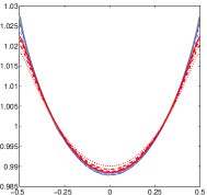
(a) Density, $\rho$

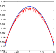
(b) Temperature, $\theta$

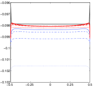
(c) Shear stress, $\sigma_{12}$

(d) Heat flux, $q_{1}$

Figure 1: Solution of the Couette flow for $\mathit{Kn}=0.1199$ with $u^{W}=1.2577$ on a uniform grid of $N=2048$.

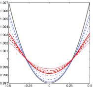
(a) Density, $\rho$

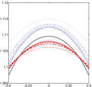
(b) Temperature, $\theta$

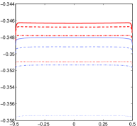
(c) Shear stress, $\sigma_{12}$

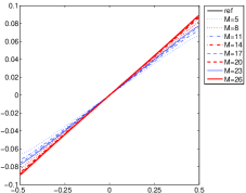
(d) Heat flux, $q_{1}$

Figure 2: Solution of the Couette flow for $\mathit{Kn}=1.199$ with $u^{W}=1.2577$ on a uniform grid of $N=2048$.

As pointed out in [8], the moment models reduce degrees of freedom significantly in comparison to the discrete velocity method that was used in [28]. While on the other hand, we have observed from our computations that as a variation of explicit time-integration scheme, the SGS-Richardson iteration converges in general several times faster, consequently more efficient, than the time-integration scheme employed in [8]. Therefore, below we only investigate the effectiveness of the multi-level strategy using lower-order model correction to accelerate the convergence and the behavior of the resulting NMLM solver. For comparison, all the computations start from the same global equilibrium with

$$\rho^{0}(x)=1,\quad\boldsymbol{u}^{0}(x)=0,\quad\theta^{0}(x)=1.$$ (35)

We perform the NMLM solver with different levels and order reduction strategies for the moment model of various orders on three uniform grids of $N=128$, $256$, $512$, respectively. Only some of numerical results are shown in this paper, since the NMLM solver exhibits similar features for all cases. In the tables given below, $K$ and $T$ represent respectively the total number and CPU seconds of the NMLM iterations to reach the steady state, while $K_{s}$ and $T_{s}$ are corresponding quantities of the single level solver.

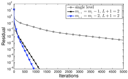
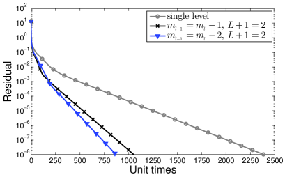
Figure 3: Convergence history of the NMLM solver for the Couette flow with $\mathit{Kn}=0.1199$, $u^{W}=1.2577$ and $M=4$ on a uniform grid of $N=512$.

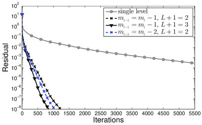
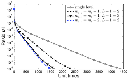
Figure 4: Convergence history of the NMLM solver for the Couette flow with $\mathit{Kn}=0.1199$, $u^{W}=1.2577$ and $M=5$ on a uniform grid of $N=512$.

First the Couette flow for $\mathit{Kn}=0.1199$ and $u^{W}=1.2577$ is considered. Table 1 gives the performance results for the case of order $M=4$ and $5$. The corresponding convergence histories on the uniform grid of $N=512$ are shown in Figure 3 for $M=4$ and in Figure 4 for $M=5$, respectively. It is quite inspiring that the NMLM solver is effective for such cases, where the order of the moment model is not very large. For both cases, the convergence is accelerated and the total computational cost, i.e., the CPU time, is reduced a lot, by the multi-level NMLM iterations, in comparison to the single level solver. It can be seen that for two-level NMLM solvers, the order reduction strategy $m_{\scriptscriptstyle l-1}=m_{\scriptscriptstyle l}-2$ converges faster than the strategy $m_{\scriptscriptstyle l-1}=m_{\scriptscriptstyle l}-1$. Moreover, the computational cost of each NMLM iteration for the former strategy is also less than the latter strategy, since the strategy $m_{\scriptscriptstyle l-1}=m_{\scriptscriptstyle l}-2$ employs a lower-order model correction with the order less than the counterpart of the strategy $m_{\scriptscriptstyle l-1}=m_{\scriptscriptstyle l}-1$. Thus, the overall performance of the strategy $m_{\scriptscriptstyle l-1}=m_{\scriptscriptstyle l}-2$ is better than the strategy $m_{\scriptscriptstyle l-1}=m_{\scriptscriptstyle l}-1$, when the same two levels is used in the NMLM solver. As the total levels up to 3, the convergence rate of the NMLM solver becomes better than both two-level NMLM solvers. Although the strategy $m_{\scriptscriptstyle l-1}=m_{\scriptscriptstyle l}-1$ becomes also more efficient as the total levels increases, the three-level NMLM solver with the strategy $m_{\scriptscriptstyle l-1}=m_{\scriptscriptstyle l}-1$ would still not be more efficient than the two-level NMLM solver with the strategy $m_{\scriptscriptstyle l-1}=m_{\scriptscriptstyle l}-2$. At last, it can also be found from Table 1 that the multi-level NMLM solver behaves similar to the single level solver as well as the explicit time-integration scheme. That is, the total number of NMLM iterations doubles and the total CPU seconds quadruples, as the grid number $N$ doubles.

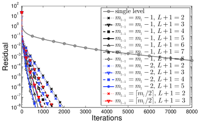
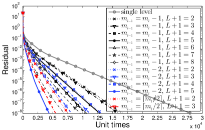
Figure 5: Convergence history of the NMLM solver for the Couette flow with $\mathit{Kn}=0.1199$, $u^{W}=1.2577$ and $M=10$ on a uniform grid of $N=512$.

For the case of order $M=10$, the performance results are listed in Table 2-3, and the corresponding convergence histories on the uniform grid of $N=512$ are shown in Figure 5. Now the order reduction strategy $m_{\scriptscriptstyle l-1}=\lceil m_{\scriptscriptstyle l}/2\rceil$ can also be applied. It can be seen again that the multi-level NMLM solvers for all three order reduction strategies could accelerate the steady-state computation. In more details, when the NMLM solvers with the same total levels are performed, the most efficient order reduction strategy is $m_{\scriptscriptstyle l-1}=\lceil m_{\scriptscriptstyle l}/2\rceil$, the second is $m_{\scriptscriptstyle l-1}=m_{\scriptscriptstyle l}-2$, and the third is $m_{\scriptscriptstyle l-1}=m_{\scriptscriptstyle l}-1$, for that they are in descending sort not only on the speed of convergence, but also on the computational cost of each NMLM iteration. As the total levels increases, both the convergence rate and the efficiency of the NMLM solver become better for each order reduction strategy. However, the $8$-level NMLM solver with the strategy $m_{\scriptscriptstyle l-1}=m_{\scriptscriptstyle l}-1$ does still less efficient than the $5$-level NMLM solver with the strategy $m_{\scriptscriptstyle l-1}=m_{\scriptscriptstyle l}-2$, whereas the overall performance of the latter solver is just close to the $3$-level NMLM solver with the strategy $m_{\scriptscriptstyle l-1}=\lceil m_{\scriptscriptstyle l}/2\rceil$, for which the total computational cost is saved by approximately more than $80\%$ in comparison to the single level solver. In addition, we have again that the total number of NMLM iterations doubles and the total CPU seconds quadruples, as the grid number $N$ doubles.

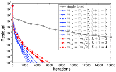
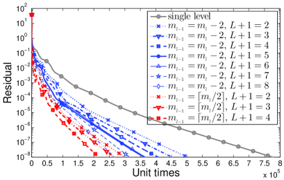
Figure 6: Convergence history of the NMLM solver for the Couette flow with $\mathit{Kn}=1.199$, $u^{W}=1.2577$ and $M=23$ on a uniform grid of $N=512$.

As mentioned previous, the moment model up to order $M=23$ or $26$ should be taken into consideration when $\mathit{Kn}=1.199$. A partial performance results are shown in Table 4 for the case of order $M=23$, and in Table 5 for the case of order $M=26$, respectively. The corresponding convergence histories are plotted in Figure 6-7. We do not present results of the NMLM solver with the strategy $m_{\scriptscriptstyle l-1}=m_{\scriptscriptstyle l}-1$ here, since compared with the single level solver it turns out a little improvement in efficiency, although the speed of convergence is raised much. This is reasonable by noting that the order of the lower-order problem just reduces $1$ at each level, for example, the order sequence for $M=26$ is $26,25,24,\ldots$, which indicates that the lower-order model correction still takes a lot of computational cost. In fact, the computational cost of lower-order model correction can not be underestimated, even when the strategy $m_{\scriptscriptstyle l-1}=m_{\scriptscriptstyle l}-2$, giving the order sequence $26,24,22,\ldots$ for $M=26$, is adopted. Moreover, it can be seen that the multi-level NMLM solver has some degeneracy, especially for the solver with the strategy $m_{\scriptscriptstyle l-1}=\lceil m_{\scriptscriptstyle l}/2\rceil$. As a result, the overall performance of the multi-level NMLM solver would not be as good as the solver when $\mathit{Kn}=0.1199$, although the efficiency is still improved much compared with the single level solver. Furthermore, unlike the observation when $\mathit{Kn}=0.1199$, the convergence rate of the strategy $m_{\scriptscriptstyle l-1}=\lceil m_{\scriptscriptstyle l}/2\rceil$ is worse than the strategy $m_{\scriptscriptstyle l-1}=m_{\scriptscriptstyle l}-2$. However, with the help of great reduction of the computational cost at each NMLM iteration, the strategy $m_{\scriptscriptstyle l-1}=\lceil m_{\scriptscriptstyle l}/2\rceil$ finally exhibits more efficient than the strategy $m_{\scriptscriptstyle l-1}=m_{\scriptscriptstyle l}-2$. On the other hand, oscillations of the residual are now observed at the beginning iterations of single level solver. For the multi-level NMLM solvers, the oscillations become more severer, and may introduce instability of the solver. Actually, the $5$-level NMLM solver with the strategy $m_{\scriptscriptstyle l-1}=\lceil m_{\scriptscriptstyle l}/2\rceil$ breaks down in our computations. In view of these, a possible way of taking both efficiency and stability into account might be to adopt the order reduction strategy $m_{\scriptscriptstyle l-1}=m_{\scriptscriptstyle l}-\delta m$, such that $\delta m>2$ and $m_{\scriptscriptstyle l}-\delta m>\lceil m_{\scriptscriptstyle l}/2\rceil$. At last, we have again that the convergence rate is improved by the multi-level NMLM solver as the total levels increases, and the multi-level NMLM solvers behave similarly to the single level solver, as the grid number $N$ doubles.

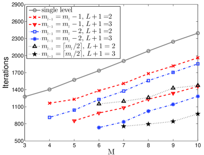
(a) $\mathit{Kn}=0.1199$

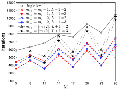
(b) $\mathit{Kn}=1.199$

Figure 8: Total iterations in terms of $M$ of the NMLM solver for the Couette flow with $u^{W}=1.2577$ on a uniform grid of $N=512$. The total iterations of the single level solver is rescaled by a factor of $12$ for $\mathit{Kn}=0.1199$ and $8$ for $\mathit{Kn}=1.199$ respectively.

It is noted from Table 4-5 that the total iterations $K$ is almost doubled as $M$ increases from $23$ to $26$, while the total iterations $K$ shown in Table 1-3 increases much slower as $M$ increases from $4$ to $10$. The significant difference is mainly due to the different performance of the smoothing operator (equivalently the single level solver) with respect to the Knudsen number $\mathit{Kn}$. To see it in more detail, we plot $K$ in terms of $M$ for the NMLM solver in Figure 8. It can be seen that the total iterations $K$ of the single level solver increases linearly with respect to $M$ for the case $\mathit{Kn}=0.1199$, whereas for the case $\mathit{Kn}=1.199$ the total iterations $K$ of the single level solver shows a strong difference with respect to the parity of $M$, especially for a larger $M$. To be specific, the total iterations $K$ increases linearly with a smaller rate with respect to odd $M$, and with a larger rate with respect to even $M$. As for the two-level and three-level NMLM solvers with the same order reduction strategy, we can see the total iterations $K$ increases linearly with similar rate with respect to $M$, in comparison to the corresponding single level solver.

In summary, it is effective to accelerate the steady-state computation by using the multi-level NMLM solver. The convergence rate would become better as the total levels increases, and the total computational cost is then saved a lot by comparing with the single level solver. Among three order reduction strategies, the strategy $m_{\scriptscriptstyle l-1}=\lceil m_{\scriptscriptstyle l}/2\rceil$ would be most efficient, followed with the strategy $m_{\scriptscriptstyle l-1}=m_{\scriptscriptstyle l}-2$, and then the strategy $m_{\scriptscriptstyle l-1}=m_{\scriptscriptstyle l}-1$.

		$M=4$			$M=5$
			$m_{\scriptscriptstyle l-1}=m_{\scriptscriptstyle l}-1$	$m_{\scriptscriptstyle l-1}=m_{\scriptscriptstyle l}-2$		$m_{\scriptscriptstyle l-1}=m_{\scriptscriptstyle l}-1$		$m_{\scriptscriptstyle l-1}=m_{\scriptscriptstyle l}-2$
$L+1$		1	2	2	1	2	3	2
$N=128$	$K$	3955	263	210	4217	261	174	228
	$T$	155.558	80.320	49.219	243.090	122.534	59.466	84.243
	$K_{s}/K$	1.0	15.038	18.833	1.0	16.157	24.236	18.496
	$T_{s}/T$	1.0	1.937	3.161	1.0	1.984	4.088	2.886
$N=256$	$K$	8178	557	440	9064	591	410	500
	$T$	633.756	348.631	209.665	1059.542	573.913	420.866	371.722
	$K_{s}/K$	1.0	14.682	18.586	1.0	15.337	22.107	18.128
	$T_{s}/T$	1.0	1.818	3.023	1.0	1.846	2.518	2.850
$N=512$	$K$	16848	1163	913	18875	1231	853	1041
	$T$	2390.169	1054.177	871.586	4433.716	2350.401	1677.407	1501.216
	$K_{s}/K$	1.0	14.487	18.453	1.0	15.333	22.128	18.132
	$T_{s}/T$	1.0	2.267	2.742	1.0	1.886	2.643	2.953

Table 1: Performance of the NMLM solver for the Couette flow with $\mathit{Kn}=0.1199$, $u^{W}=1.2577$ and $M=4,5$.

		$m_{\scriptscriptstyle l-1}=m_{\scriptscriptstyle l}-1$
$L+1$		2	3	4	5	6	7	8
$N=128$	$K$	476	354	276	224	189	168	156
	$T$	1287.045	1012.705	908.478	773.019	681.257	617.487	573.095
	$K_{s}/K$	14.639	19.684	25.246	31.107	36.868	41.476	44.667
	$T_{s}/T$	1.481	1.882	2.097	2.465	2.797	3.086	3.325
$N=256$	$K$	963	716	560	454	380	332	303
	$T$	4693.688	3787.012	3767.613	3176.846	2716.522	2189.956	2216.659
	$K_{s}/K$	14.652	19.707	25.196	31.079	37.132	42.500	46.568
	$T_{s}/T$	1.810	2.243	2.255	2.674	3.127	3.879	3.833
$N=512$	$K$	1961	1457	1139	921	768	663	597
	$T$	16760.802	16049.136	10434.860	12920.731	10710.200	9641.965	6954.572
	$K_{s}/K$	14.651	19.719	25.224	31.194	37.409	43.333	48.124
	$T_{s}/T$	1.681	1.756	2.700	2.181	2.631	2.922	4.051

Table 2: Performance of the NMLM solver for the Couette flow with $\mathit{Kn}=0.1199$, $u^{W}=1.2577$ and $M=10$ (part I).

		$m_{\scriptscriptstyle l-1}=m_{\scriptscriptstyle l}-2$				$m_{\scriptscriptstyle l-1}=\lceil m_{\scriptscriptstyle l}/2\rceil$
$L+1$		2	3	4	5	2	3	1
$N=128$	$K$	450	312	221	165	357	237	6968
	$T$	789.648	597.272	497.074	363.046	531.005	334.993	1905.477
	$K_{s}/K$	15.484	22.333	31.529	42.230	19.518	29.401	1.0
	$T_{s}/T$	2.413	3.190	3.833	5.249	3.588	5.688	1.0
$N=256$	$K$	912	631	446	327	724	479	14110
	$T$	4233.031	2572.533	2004.516	1445.255	1951.228	1356.081	8495.687
	$K_{s}/K$	15.471	22.361	31.637	43.150	19.489	29.457	1.0
	$T_{s}/T$	2.007	3.302	4.238	5.878	4.354	6.265	1.0
$N=512$	$K$	1855	1283	903	651	1474	975	28730
	$T$	13206.382	11231.685	8146.139	4405.231	7564.141	5498.801	28174.869
	$K_{s}/K$	15.488	22.393	31.816	44.132	19.491	29.467	1.0
	$T_{s}/T$	2.133	2.509	3.459	6.396	3.725	5.124	1.0

Table 3: Performance of the NMLM solver for the Couette flow with $\mathit{Kn}=0.1199$, $u^{W}=1.2577$ and $M=10$ (part II).

		$m_{\scriptscriptstyle l-1}=m_{\scriptscriptstyle l}-2$					$m_{\scriptscriptstyle l-1}=\lceil m_{\scriptscriptstyle l}/2\rceil$
$L+1$		4	5	6	7	8	2	3	4
$N=128$	$K$	796	660	481	506	530	1440	1440	1338
	$T$	26508.912	22966.565	17201.641	17694.056	13069.990	18894.415	19519.867	10330.927
	$K_{s}/K$	16.991	20.492	28.119	26.729	25.519	9.392	9.392	10.108
	$T_{s}/T$	1.165	1.345	1.796	1.746	2.364	1.635	1.583	2.991
$N=256$	$K$	1593	1386	1220	1099	1007	2405	2602	2409
	$T$	105550.167	96564.039	86944.937	79480.186	57305.984	62363.809	72069.420	65186.066
	$K_{s}/K$	16.559	19.032	21.621	24.002	26.195	10.968	10.138	10.950
	$T_{s}/T$	1.396	1.526	1.694	1.854	2.571	2.362	2.044	2.260
$N=512$	$K$	3392	2998	2717	2511	2353	5979	5295	5074
	$T$	408209.027	363005.320	366497.127	316449.369	268045.359	300242.049	266417.091	216497.893
	$K_{s}/K$	19.268	21.801	24.055	26.029	27.776	10.931	12.343	12.881
	$T_{s}/T$	1.903	2.140	2.119	2.455	2.898	2.587	2.915	3.588

Table 4: Performance of the NMLM solver for the Couette flow with $\mathit{Kn}=1.199$, $u^{W}=1.2577$ and $M=23$.

		$m_{\scriptscriptstyle l-1}=m_{\scriptscriptstyle l}-2$					$m_{\scriptscriptstyle l-1}=\lceil m_{\scriptscriptstyle l}/2\rceil$
$L+1$		4	5	6	7	8	2	3	4
$N=128$	$K$	1559	1472	1410	1363	1326	2627	2496	2405
	$T$	67950.969	73383.501	58109.432	76334.248	68269.101	48025.102	47618.776	46879.272
	$K_{s}/K$	13.528	14.327	14.957	15.473	15.905	8.028	8.450	8.769
	$T_{s}/T$	1.124	1.041	1.315	1.001	1.119	1.591	1.605	1.630
$N=256$	$K$	3083	2911	2789	2696	2622	5190	4920	4715
	$T$	276985.452	297746.135	296101.816	275546.571	212048.261	211041.390	194471.039	178270.975
	$K_{s}/K$	13.586	14.389	15.019	15.537	15.975	8.071	8.514	8.884
	$T_{s}/T$	1.265	1.177	1.183	1.271	1.652	1.660	1.801	1.965
$N=512$	$K$	6116	5778	5536	5354	5207	10303	9761	9319
	$T$	1147507.284	887609.149	992797.036	889783.318	801075.758	607645.946	663480.962	555586.099
	$K_{s}/K$	13.664	14.463	15.095	15.609	16.049	8.111	8.561	8.967
	$T_{s}/T$	1.158	1.497	1.338	1.493	1.658	2.186	2.002	2.391

Table 5: Performance of the NMLM solver for the Couette flow with $\mathit{Kn}=1.199$, $u^{W}=1.2577$ and $M=26$.

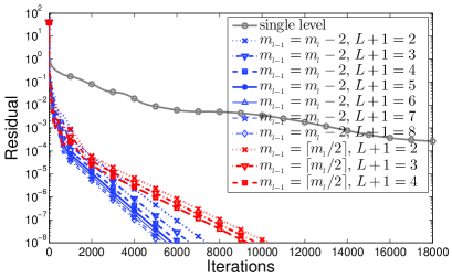
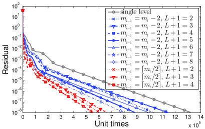
Figure 7: Convergence history of the NMLM solver for the Couette flow with $\mathit{Kn}=1.199$, $u^{W}=1.2577$ and $M=26$ on a uniform grid of $N=512$.

4.2 The force driven Poiseuille flow

The force driven Poiseuille flow is another benchmark test frequently investigated in the literatures [35, 7, 34, 19]. Similar to the Couette flow, there are two infinite parallel plates, which are separated by a distance of $L=1$, and have the same temperature of $\theta^{W}=1$. However, both plates are stationary now, and the gas between them is driven by an external constant force, which is set as $\boldsymbol{F}=(0,0.2555,0)^{T}$ in our tests. Additionally, the collision frequency $\nu$ is given by the hard sphere model as

$$\nu=\frac{16}{5}\sqrt{\frac{\theta}{2\pi}}\frac{\Pr}{\mathit{Kn}}\rho,$$ (36)

and the Knudsen number $\mathit{Kn}=0.1$ is considered. With these settings, the steady-state solution obtained by the NMLM solver is shown in Figure 9, which recovers exactly the steady-state solution presented in [19].

We still omit the discussion on the accuracy and the convergence of the solution with respect to order $M$, and focus on the behavior of the proposed NMLM solver. As the Couette flow, the NMLM solvers, with different levels and order reduction strategies for the moment model of various orders on three uniform grids of $N=128$, $256$, $512$, are performed. The computations also begin with the global equilibrium (35). Again just partial numerical results are shown here, for similar features can be observed for all cases. To be specific, the performance results are given in Table 6 for the case of order $M=4$, $5$, and in Table 7-8 for the case of order $M=10$, respectively. The corresponding convergence histories on the uniform grid of $N=512$ are displayed respectively in Figure 10 for $M=4$, in Figure 11 for $M=5$, and in Figure 12 for $M=10$. The total iterations $K$ in terms of $M$ for the NMLM solver is presented in Figure 13. All these results show that the multi-level NMLM solver is able to accelerate the steady-state computation significantly.

In comparison to results of the Couette flow with $\mathit{Kn}=0.1199$, a similar behavior of the multi-level NMLM solver can be observed. In more details, we can see that the most efficient order reduction strategy is $m_{\scriptscriptstyle l-1}=\lceil m_{\scriptscriptstyle l}/2\rceil$, the second is $m_{\scriptscriptstyle l-1}=m_{\scriptscriptstyle l}-2$, and the third is $m_{\scriptscriptstyle l-1}=m_{\scriptscriptstyle l}-1$. As can be seen from the tables, the ratio of $K_{s}$ and $K$ are all consistent with those for the Couette flow. Consequently, the convergence rate of the multi-level NMLM solver with all three order reduction strategies increase as the total levels increases, and the total computational cost is saved greatly in comparison to the single level solver. In addition, as the grid number $N$ doubles, all multi-level NMLM solver show similar features as the single level solver. Thus, the acceleration ratio will be maintained even when a more fine spatial grid is adopted.

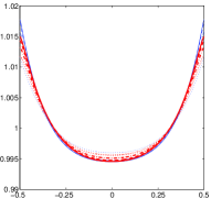
(a) Density, $\rho$

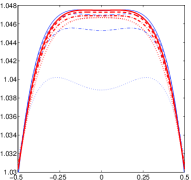
(b) Temperature, $\theta$

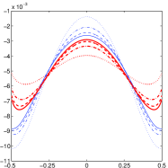
(c) Normal stress, $\sigma_{11}$

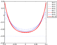
(d) Heat flux, $q_{2}$

Figure 9: Solution of the force driven Poiseuille flow on a uniform grid of $N=2048$.

		$M=4$			$M=5$
			$m_{\scriptscriptstyle l-1}=m_{\scriptscriptstyle l}-1$	$m_{\scriptscriptstyle l-1}=m_{\scriptscriptstyle l}-2$		$m_{\scriptscriptstyle l-1}=m_{\scriptscriptstyle l}-1$		$m_{\scriptscriptstyle l-1}=m_{\scriptscriptstyle l}-2$
$L+1$		1	2	2	1	2	3	2
$N=128$	$K$	6660	405	330	7627	490	334	416
	$T$	168.395	73.819	80.196	300.558	140.285	156.427	111.988
	$K_{s}/K$	1.0	16.444	20.182	1.0	15.565	22.835	18.334
	$T_{s}/T$	1.0	2.281	2.100	1.0	2.142	1.921	2.684
$N=256$	$K$	14111	855	699	16219	1040	709	883
	$T$	729.814	502.633	338.805	1270.682	837.806	757.453	677.226
	$K_{s}/K$	1.0	16.504	20.187	1.0	15.595	22.876	18.368
	$T_{s}/T$	1.0	1.452	2.154	1.0	1.517	1.678	1.876
$N=512$	$K$	29077	1756	1441	33653	2157	1470	1832
	$T$	2915.750	2113.058	1094.692	6382.696	3276.133	3036.576	2181.178
	$K_{s}/K$	1.0	16.559	20.178	1.0	15.602	22.893	18.370
	$T_{s}/T$	1.0	1.380	2.664	1.0	1.948	2.102	2.926

Table 6: Performance of the NMLM solver for the Poiseuille flow with $M=4,5$.

		$m_{\scriptscriptstyle l-1}=m_{\scriptscriptstyle l}-1$
$L+1$		2	3	4	5	6	7	8
$N=128$	$K$	763	566	441	352	286	233	188
	$T$	1579.371	1469.207	873.198	1246.409	1037.293	872.312	705.808
	$K_{s}/K$	14.667	19.772	25.376	31.793	39.129	48.030	59.527
	$T_{s}/T$	1.497	1.610	2.708	1.897	2.280	2.711	3.351
$N=256$	$K$	1680	1247	970	776	630	514	414
	$T$	6771.226	6871.824	5150.564	3965.397	3738.700	3824.224	3020.587
	$K_{s}/K$	14.674	19.769	25.414	31.768	39.130	47.961	59.546
	$T_{s}/T$	1.864	1.837	2.451	3.183	3.376	3.301	4.179
$N=512$	$K$	3560	2642	2056	1646	1336	1089	877
	$T$	30046.298	24663.853	19606.473	19143.007	15356.107	11740.206	11755.468
	$K_{s}/K$	14.678	19.779	25.416	31.747	39.113	47.984	59.584
	$T_{s}/T$	1.608	1.959	2.465	2.524	3.147	4.116	4.111

Table 7: Performance of the NMLM solver for the Poiseuille flow with $M=10$ (part I).

		$m_{\scriptscriptstyle l-1}=m_{\scriptscriptstyle l}-2$				$m_{\scriptscriptstyle l-1}=\lceil m_{\scriptscriptstyle l}/2\rceil$
$L+1$		2	3	4	5	2	3	1
$N=128$	$K$	722	498	346	217	569	340	11191
	$T$	1683.538	1014.106	753.820	483.238	881.392	371.769	2364.837
	$K_{s}/K$	15.500	22.472	32.344	51.571	19.668	32.915	1.0
	$T_{s}/T$	1.405	2.332	3.137	4.894	2.683	6.361	1.0
$N=256$	$K$	1590	1098	761	478	1253	750	24652
	$T$	6355.823	4845.505	2014.658	1982.888	2369.244	2227.680	12623.650
	$K_{s}/K$	15.504	22.452	32.394	51.573	19.674	32.869	1.0
	$T_{s}/T$	1.986	2.605	6.266	6.366	5.328	5.667	1.0
$N=512$	$K$	3370	2326	1613	1014	2656	1589	52255
	$T$	21037.239	13185.407	10524.655	8432.436	14278.116	7782.965	48320.953
	$K_{s}/K$	15.506	22.466	32.396	51.534	19.674	32.885	1.0
	$T_{s}/T$	2.297	3.665	4.591	5.730	3.384	6.209	1.0

Table 8: Performance of the NMLM solver for the Poiseuille flow with $M=10$ (part II).

Figure 10: Convergence history of the NMLM solver for the Poiseuille flow with $M=4$ on a uniform grid of $N=512$.

Figure 11: Convergence history of the NMLM solver for the Poiseuille flow with $M=5$ on a uniform grid of $N=512$.

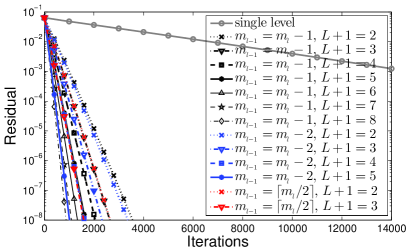
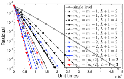
Figure 12: Convergence history of the NMLM solver for the Poiseuille flow with $M=10$ on a uniform grid of $N=512$.

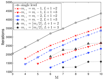
Figure 13: Total iterations in terms of $M$ of the NMLM solver for the Poiseuille flow on a uniform grid of $N=512$. The total iterations of the single level solver is rescaled by a factor of $12$.

5 Concluding remarks

The acceleration for the steady-state computation of the high-order moment model by using the lower-order model correction has been investigated in this paper. A nonlinear multi-level moment solver which has unified framework for the moment model of arbitrary order is then developed. The convergence rate would be improved as the total levels of the NMLM solver increases. It is demonstrated by numerical experiments of two benchmark problems that the proposed NMLM solver improves the convergence rate significantly and the total computational cost could be saved a lot, in comparison to the single level solver. Three order reduction strategies for the lower-order model correction are also considered. It turns out that the most efficient strategy is $m_{\scriptscriptstyle l-1}=\lceil m_{\scriptscriptstyle l}/2\rceil$, the second is $m_{\scriptscriptstyle l-1}=m_{\scriptscriptstyle l}-2$, and the third is $m_{\scriptscriptstyle l-1}=m_{\scriptscriptstyle l}-1$.

It should be pointed out that the NMLM solver does not as efficient as the nonlinear multigrid solver developed in [19]. However, we have that the spatial grid for our NMLM solver is unchanged at each level, and the acceleration ratio obtained by the NMLM solver would be maintained on different spatial grid. Then a natural way of obtaining a more efficient steady-state solver might be to combine both NMLM iteration and nonlinear multigrid iteration together. This will be investigated in our futural work.

References

- [1] P. L. Bhatnagar, E. P. Gross, and M. Krook. A model for collision processes in gases. I. small amplitude processes in charged and neutral one-component systems. Phys. Rev., 94(3):511–525, 1954.
- [2] A. Brandt and O. E. Livne. Multigrid Techniques: 1984 Guide with Applications to Fluid Dynamics. Classics in Applied Mathematics. SIAM, revised edition, 2011.
- [3] Z. Cai, Y. Fan, and R. Li. Globally hyperbolic regularization of Grad’s moment system in one dimensional space. Comm. Math. Sci., 11(2):547–571, 2013.
- [4] Z. Cai, Y. Fan, and R. Li. Globally hyperbolic regularization of Grad’s moment system. Comm. Pure Appl. Math., 67(3):464–518, 2014.
- [5] Z. Cai, Y. Fan, and R. Li. A framework on moment model reduction for kinetic equation. SIAM J. Appl. Math., 75(5):2001–2023, 2015.
- [6] Z. Cai and R. Li. Numerical regularized moment method of arbitrary order for Boltzmann-BGK equation. SIAM J. Sci. Comput., 32(5):2875–2907, 2010.
- [7] Z. Cai, R. Li, and Z. Qiao. NR simulation of microflows with Shakhov model. SIAM J. Sci. Comput., 34(1):A339–A369, 2012.
- [8] Z. Cai, R. Li, and Z. Qiao. Globally hyperbolic regularized moment method with applications to microflow simulation. Computers and Fluids, 81:95–109, 2013.
- [9] Z. Cai, R. Li, and Y. Wang. An efficient NR method for Boltzmann-BGK equation. J. Sci. Comput., 50(1):103–119, 2012.
- [10] Z. Cai, R. Li, and Y. Wang. Numerical regularized moment method for high Mach number flow. Commun. Comput. Phys., 11(5):1415–1438, 2012.
- [11] Z. Cai, R. Li, and Y. Wang. Solving Vlasov equation using NR method. SIAM J. Sci. Comput., 35(6):A2807–A2831, 2013.
- [12] S. Chapman and T. G. Cowling. The Mathematical Theory of Non-uniform Gases, Third Edition. Cambridge University Press, 1990.
- [13] K. J. Fidkowski, T. A. Oliver, J. Lu, and D. L. Darmofal. -Multigrid solution of high-order discontinuous Galerkin discretizations of the compressible Navier-Stokes equations. J. Comput. Phys., 207(1):92–113, Jul 2005.
- [14] H. Grad. On the kinetic theory of rarefied gases. Comm. Pure Appl. Math., 2(4):331–407, 1949.
- [15] W. Hackbusch. Multi-Grid Methods and Applications. Springer-Verlag, Berlin, 1985. second printing 2003.
- [16] B. T. Helenbrook and H. L. Atkins. Solving discontinuous Galerkin formulations of Poisson’s equation using geometric and multigrid. AIAA Journal, 46(4):894–902, Apr 2008.
- [17] L. H. Holway. New statistical models for kinetic theory: Methods of construction. Phys. Fluids, 9(1):1658–1673, 1966.
- [18] G. H. Hu, R. Li, and T. Tang. A robust high-order residual distribution type scheme for steady Euler equations on unstructured grids. J. Comput. Phys., 229:1681–1697, 2010.
- [19] Z. Hu and R. Li. A nonlinear multigrid steady-state solver for 1D microflow. Computers and Fluids, 103:193–203, 2014.
- [20] Z. Hu, R. Li, T. Lu, Y. Wang, and W. Yao. Simulation of an -- diode by using globally-hyperbolically-closed high-order moment models. J. Sci. Comput., 59(3):761–774, 2014.
- [21] Z. Hu, R. Li, and Z. Qiao. Extended hydrodynamic models and multigrid solver of a silicon diode simulation. Commun. Comput. Phys., 20(3):551–582, Sep 2016.
- [22] R. Kannan. An implicit LU-SGS spectral volume method for the moment models in device simulations: Formulation in 1D and application to a p-multigrid algorithm. Int. J. Numer. Meth. Biomed. Engng., 27:1362–1375, 2011.
- [23] R. Li, X. Wang, and W.-B. Zhao. A multigrid block LU-SGS algorithm for Euler equations on unstructured grids. Numer. Math. Theor. Meth. Appl., 1(1):92–112, 2008.
- [24] H. Luo, J. D. Baum, and R. Löhner. Fast -multigrid discontinuous Galerkin method for compressible flows at all speeds. AIAA Journal, 46(3):635–652, Mar 2008.
- [25] Y. Maday and R. Muñoz. Spectral element multigrid. II. Theoretical justification. J. Sci. Comput., 3(4):323–353, 1988.
- [26] B. S. Mascarenhas, B. T. Helenbrook, and H. L. Atkins. Coupling -multigrid to geometric multigrid for discontinuous Galerkin formulations of the convection-diffusion equation. J. Comput. Phys., 229(10):3664–3674, May 2010.
- [27] D. J. Mavriplis. An assessment of linear versus nonlinear multigrid methods for unstructured mesh solvers. J. Comput. Phys., 175:302–325, 2002.
- [28] L. Mieussens and H. Struchtrup. Numerical comparison of Bhatnagar-Gross-Krook models with proper Prandtl number. Phys. Fluids, 16(8):2797–2813, 2004.
- [29] E. M. Rønquist and A. T. Patera. Spectral element multigrid. I. Formulation and numerical results. J. Sci. Comput., 2(4):389–406, 1987.
- [30] E. M. Shakhov. Generalization of the Krook kinetic relaxation equation. Fluid Dyn., 3(5):95–96, 1968.
- [31] R. Speck, D. Ruprecht, M. Emmett, M. Minion, M. Bolten, and R. Krause. A multi-level spectral deferred correction method. BIT Numer. Math., 55:843–867, 2015.
- [32] H. Struchtrup. Macroscopic Transport Equations for Rarefied Gas Flows: Approximation Methods in Kinetic Theory. Springer, 2005.
- [33] M. Wallraff, R. Hartmann, and T. Leicht. Multigrid solver algorithms for DG methods and applications to aerodynamic flows. In N. Kroll, C. Hirsch, F. Bassi, C. Johnston, and K. Hillewaert, editors, IDIHOM: Industrialization of High-Order Methods - A Top-Down Approach, volume 128 of Notes on Numerical Fluid Mechanics and Multidisciplinary Design, pages 153–178. Springer International Publishing, 2015.
- [34] K. Xu, H. Liu, and J. Jiang. Multiple-temperature model for continuum and near continuum flows. Phys. Fluids, 19(1):016101, 2007.
- [35] Y. Zheng, A. L. Garcia, and B. J. Alder. Comparison of kinetic theory and hydrodynamics for Poiseuille flow. J. Stat. Phys., 109(3–4):495–505, 2002.