Structure and kinematics of the clouds surrounding
the Galactic mini-starburst W43 MM1

Massive stars have a major influence on their environment yet their formation is difficult to study as they form quickly in highly obscured regions and are rare, hence more distant than lower mass stars. W43 is a highly luminous galactic massive star forming region at a distance of 5.5 kpc and the MM1 part hosts a particularly massive dense core (1000 M_⊙within 0.05 pc). We present new Herschel HIFI maps of the W43 MM1 region covering the main low-energy water lines at 557, 987, and 1113 GHz, their H${}_{2}^{18}$O counterparts, and other lines such as ¹³CO (10-9) and C¹⁸O (9-8) which trace warm gas. These water lines are, with the exception of line wings, observed in absorption. Herschel SPIRE and JCMT $450\,\mbox{$\mu$m}$ data have been used to make a model of the continuum emission at the HIFI wavelengths. Analysis of the maps, and in particular the optical depth maps of each line and feature, shows that a velocity gradient, possibly due to rotation, is present in both the envelope ($r\lower 2.15277pt\hbox{$\;\buildrel>\over{\sim}\;$}0.5$ pc) and the protostellar core ($r\lower 2.15277pt\hbox{$\;\buildrel<\over{\sim}\;$}0.2$ pc). Velocities increase in both components from SW to NE, following the general source orientation. While the H₂O lines trace essentially the cool envelope, we show that the envelope cannot account for the H${}_{2}^{18}$O absorption, which traces motions close to the protostar. The core has rapid infall, $2.9{\rm\ km\ s^{-1}}$, as manifested by the H${}_{2}^{18}$O absorption features which are systematically red-shifted with respect to the ¹³CO (10-9)  emission line which also traces the inner material with the same angular resolution. Some H${}_{2}^{18}$O absorption is detected outside the central core and thus outside the regions expected (from a spherical model) to be above 100 K– we attribute this to warm gas associated with the other massive dense cores in W43 MM1. Using the maps to identify absorption from cool gas on large scales, we subtract this component to model spectra for the inner envelope. Modeling the new, presumably corrected, spectra results in a lower water abundance, decreased from 8 $10^{-8}$ to 8 $10^{-9}$ , with no change in infall rate.

1 Introduction

Massive star formation is still poorly understood and, while various means have been proposed to overcome the radiation pressure problem, observational ambiguities remain (see reviews by Zinnecker & Yorke 2007; Beuther et al. 2007). Massive dense cores are generally fairly distant and their centers always extremely embedded, making them difficult to observe with the necessary detail. In addition, the protostellar phase appears very short (a few $10^{5}$ years, Tan et al. 2014; Beuther et al. 2007), further reducing the number of objects. A main question is how to ”feed” a massive protostar, particularly in the earliest phases when it is weak in the infrared.

Understanding high-mass star formation is one of the goals of the Water In Star forming regions with Herschel program (WISH, Van Dishoeck et al. 2011). Water is a potentially very abundant molecule but the vast majority of water is found as ice, which cannot be used to study kinematics. Only when the temperature reaches 100 K is the water ice on dust grains vaporized, provoking a radical change in water vapor abundance from some $10^{-8}$ to $1-10\times 10^{-5}$ (Van der Tak et al. 2010; Herpin et al. 2012). This jump in abundance makes it possible in principle to use the water molecule to focus on the central regions. High-energy transitions of other molecules also come from the dense and warm central regions. However, low-energy water transitions can be observed in both emission and absorption coming from the central regions, allowing potentially infalling cooler material to be detected in absorption, unlike in high-energy transitions (Van der Tak et al. 2013).

This idealized picture does not hold for the main water isotope as even the low-abundance gas is highly optically thick. However, for the H${}_{2}^{18}$O and H${}_{2}^{17}$O isotopomers with typical abundances of respectively 450 and 2000 times lower than the main isotope, the above picture should be more appropriate. The goal of this paper is to map W43 MM1 surroundings with a large set of lines to develop a more precise image of the amount of turbulence, infall rate, and rotation in the central core but also in the cooler surrounding material. As part of this, we try to identify the lines that best allow us to study the inner and outer parts of the protostellar envelope.

W43 MM1 is a high-mass proto-stellar object situated at about 5.5 kpc from the sun (Zhang et al. 2014) at the near end of the Galactic bar. W43 is sometimes considered to be a ”mini-starburst” region because of the currently high level of star formation occurring there (Motte et al. 2003), probably due to a cloud collision (Nguyen-Lu’o’ng et al. 2013). Herschel observations, including water lines, towards the center of W43 MM1 were analyzed by Herpin et al. (2012), who present a spherically symmetric model for the structure of W43 MM1 showing that both accretion and radially increasing turbulent velocities are required. They estimate the water abundances to be $8\times 10^{-8}$ where $T_{mb}<100$ K and $1.4\times 10^{-4}$ in the warm regions, higher than in most cores (Chavarría et al. 2010). The water abundance in cold outer envelopes is usually lower, of order $10^{-9}$ – $10^{-10}$ (Van Dishoeck et al. 2013).

The general source structure is shown in Figure 1 of Louvet et al. (2014): a double central core (N1a and N1b) surrounded by an elongated structure with a column density of $\sim 10^{23}$ cm^-2. Louvet et al. (2014) found a number of Massive Dense Cores (MDC) in W43 MM1, mostly aligned to the NE and SW of the main core with a typical separation of about 5 to $10\,\arcsec$. The maps presented in this work cover the region with the cluster of MDCs identified by Louvet et al. (2014, Figure 1). The main MDC (N1) dominates the cluster, with an estimated mass of 2100 M_⊙, with the other MDC masses decreasing to typically 100 M_⊙ away from the center of the cluster. All of the MDCs identified by Louvet et al. (2014) in W43 appear overdense compared to other dense cores, such that they are likely to contain protostellar objects. Thus, the central spherically symmetric model may not well represent the source structure given the presence of heating sources – the MDCs – distributed over roughly an arcminute, particularly to the South West of the center of W43 MM1.

As part of the WISH project, W43 MM1 was mapped with the HIFI heterodyne spectrometer aboard the Herschel Space Observatory (Pilbratt et al. 2010; Roelfsema et al. 2012) at 557, 987, and 1113 GHz. These frequencies correspond to the o-H₂O 1₁₀-1₀₁, p-H₂O 2₀₂-1₁₁, and p-H₂O 1₁₁-0₀₀ water lines but also allow detection of the o-H${}_{2}^{18}$O 1₁₀-1₀₁, C¹⁸O $9-8$, p-H${}_{2}^{18}$O 1₁₁-0₀₀, and ¹³CO $10-9$ lines. The water lines (all isotopes), show a mixture of emission and absorption while the CO isotopic lines are only seen in emission. Coupled with the spatial variations, this information is used to develop a more comprehensive model of the core and envelope structure and gas motions such as infall, turbulence, and/or rotation.

2 Observations

W43 MM1 was mapped at 557, 987, and 1113 GHz using the HIFI instrument (de Graauw et al. 2010), corresponding to the o-H₂O 1₁₀-1₀₁, p-H₂O 2₀₂-1₁₁, and p-H₂O 1₁₁-0₀₀ lines. The data were taken on October 27th, 2010 (obsid 1342219193), March 11th, 2011 (obsid 1342215899), and April 21st, 2011 (obsid 1342207373). The H and V polarizations were observed simultaneously using both the acousto-optical Wide-Band Spectrometer (WBS) with 1.1 MHz resolution and the digital auto-correlator High-Resolution Spectrometer (HRS) at higher spectral resolution. We used the On-The-Fly mapping mode with Nyquist sampling and a reference position (RA${}_{OFF}=$18h48min27s, DEC${}_{OFF}=-1^{\circ}44\arcmin 28\arcsec$). The o-H₂O 1₁₀-1₀₁ line was mapped (map size $0.92\arcmin\times 1.74\arcmin$) simultaneously with the o-H${}_{2}^{18}$O 1₁₀-1₀₁ line in the lower sideband while the p-H₂O 2₀₂-1₁₁ line was mapped ($1.27\arcmin\times 1.60\arcmin$) with the C¹⁸O $9-8$ in the same upper sideband. The third map ($1.35\arcmin\times 1.68\arcmin$) combined the p-H₂O 1₁₁-0₀₀, p-H${}_{2}^{18}$O 1₁₁-0₀₀, and ¹³CO $10-9$ lines. The (0,0) position of all the maps is $\alpha_{J2000}=18^{h}47^{m}47.0^{s},\delta_{J2000}=-1^{\circ}54\arcmin 28\arcsec$. The observations are part of the WISH GT-KP (Van Dishoeck et al. 2011).

The three maps (see Table 1 ) were obtained using an On-The-Fly mapping procedure with spectra drifting along the declination axis on columns separated by a step chosen from the beam size of the main water line frequency. The pointing slightly differs between the H and the V receivers. For p-H₂O 1₁₁-0₀₀, the offset is of about 3 $\arcsec$ in Right Ascension whereas the On-The-Fly Right Ascension step is 9 $\arcsec$. As a consequence we have two maps shifted in Right Ascension by one third of the Right Ascension step. For spectra with a low continuum level, the signal to noise ratio of the individual spectra is too low to have a good detection of the absorption features. In order to improve this signal to noise ratio, we then decided to produce an almost regular grid of averaged spectra by dividing the mapped area into cells on a regular grid. We averaged all spectra within a cell, both in intensity and position.

The off position has been inspected for each targeted frequency and does not show any emission. The frequencies, energy of the upper levels, system temperatures, integration times and rms noise level at a given spectral resolution for each of the lines are provided in Table 1. Calibration of the raw data into the $T_{A}$ scale was performed by the in-orbit system (Roelfsema et al. 2012); conversion to $T_{mb}$ was done using the latest beam efficiency estimate from October 2014 given in Table 1 and a forward efficiency of 0.96. HIFI receivers are double sideband with a sideband ratio close to unity (Roelfsema et al. 2012). The flux scale accuracy is estimated to be 10% for band 1 and 15% for band 4¹. The frequency calibration accuracy is 20 kHz and 100 kHz, respectively for HRS and WBS observations. Data calibration was performed in the Herschel Interactive Processing Environment (HIPE, Ott 2010) version 13. Further analysis was done within the CLASS package. These lines are not expected to be polarized, thus, after inspection, data from the two polarizations were averaged together.

Table 1: Herschel/HIFI mapped water line transitions towards W43 MM1. Frequencies are from Pearson et al. (1991). The rms is the noise at $\delta\nu=1.1$MHz.

Setting	Transition	Frequency	$E_{u}$	Beam	Map size	$\eta_{\textrm{mb}}$	$T_{\textrm{sys}}$	rms
map (band)		[GHz]	[K]	[″]	[′]		[K]	[mK]
1 (1a)	o-H${}_{2}^{18}$O 110-101	547.6764	60.5	37.8	0.92$\times$1.74	0.62	80	27
1 (1a)	o-H2O 110-101	556.9361	61.0	37.1
2 (4a)	p-H2O 202-111	987.9268	100.8	21.3	1.27$\times$1.60	0.63	340	79
2 (4a)	C18O $9-8$	987.5604	237.0	21.3
3 (4b)	p-H${}_{2}^{18}$O 111-000	1101.6982	52.9	19.9	1.35$\times$1.6	0.63	390	20
3 (4b)	p-H2O 111-000	1113.3430	53.4	19.7
3 (4b)	13CO $10-9$	1101.3497	290.8	19.9

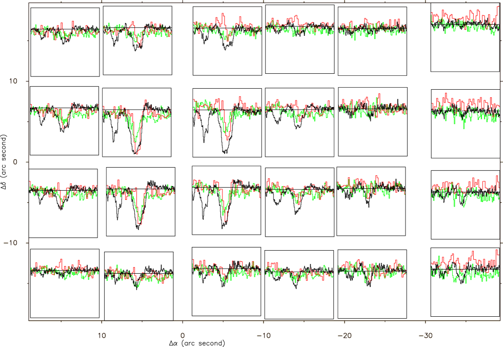
Figure 1: Map of observed spectra towards W43 MM1 for lines p-H₂O 1₁₁-0₀₀ (black, $T_{mb}=[-2.2,\,1.00]$ K), p-H${}_{2}^{18}$O 1₁₁-0₀₀ (red, $T_{mb}=[-0.55,\,0.25]$ K), and ¹³CO (10-9) (green, $T_{mb}=[1.0,\,-0.50]$ K, inverted T scale in order to ease comparisons). Velocity range: $V_{lsr}=[70,\,130]\,{\rm\ km\ s^{-1}}$. Plotted spectra are an average of OTF individual spectra around each box central position. The continuum level is subtracted.

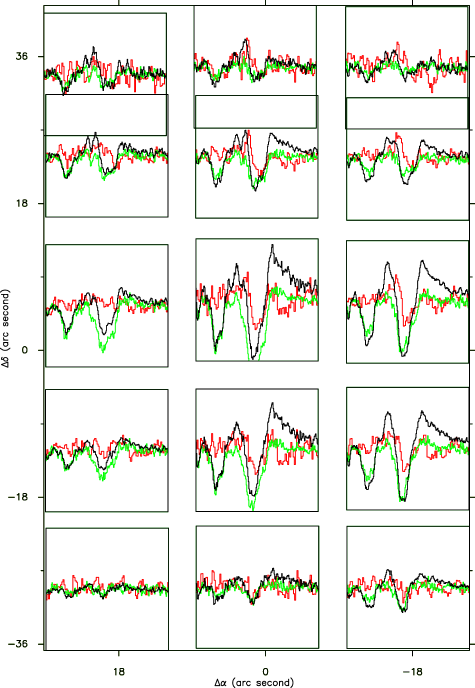
Figure 2: Map of observed spectra towards W43 MM1 for lines o-H₂O 1₁₀-1₀₁ (black, $T_{mb}=[-0.5,\,0.5]{\rm\,K}$), p-H₂O 1₁₁-0₀₀ (green, $T_{mb}=[1.0,\,1.0]{\rm\,K}$), and o-H${}_{2}^{18}$O 1₁₀-1₀₁ (red, $T_{mb}=[-0.15,\,0.15]{\rm\,K}$). Velocity range: $V_{lsr}=[75,\,130]{\rm\ km\ s^{-1}}$. The plotted spectra are an average of OTF individual spectra around each box central position. The continuum level is subtracted. Axis units are offset ($\arcsec$) from MM1.

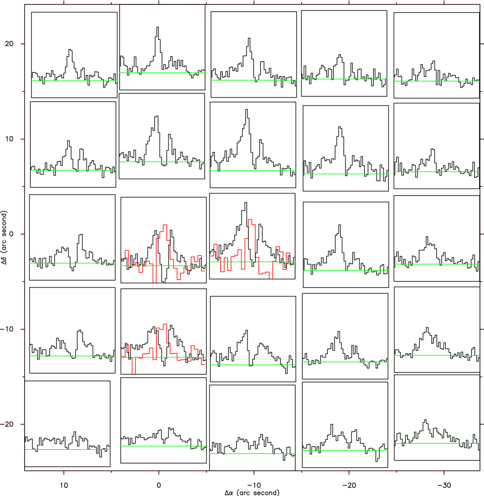
Figure 3: Map of observed spectra towards W43 MM1 for lines p-H₂O 2₀₂-1₁₁ (black, $T_{mb}=[-0.3,\,1.2]$ K) and C¹⁸O (9-8) (red, $T_{mb}=[-0.1,\,0.4]$ K). We only plotted the three C¹⁸O (9-8) spectra with a signal to noise ratio good enough. Velocity range: $V_{lsr}=[70,\,130]{\rm\ km\ s^{-1}}$ . Plotted spectra are an average of OTF individual spectra around each box central position. The continuum level is subtracted. Axis units are offset ($\arcsec$) from MM1.

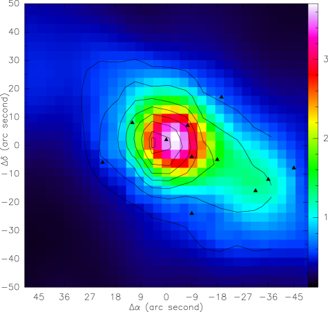
Figure 4: Maps of the W43 MM1 continuum level at $250\text{\,}\mathrm{\SIUnitSymbolMicro m}$ (SPIRE data) and at 1113 GHz ($\simeq$$269\text{\,}\mathrm{\SIUnitSymbolMicro m}$) before the offset correction. HIFI contour levels: 0.6 1.0 1.5 2.0 3.0 3.5 3.65  K with original data positions but after continuum level correction (see text). The SPIRE data (in K) resolution is smoothed to the $20\arcsec$ beam size of p-H₂O 1₁₁-0₀₀. Black triangles indicate the Louvet et al 2014 sources.

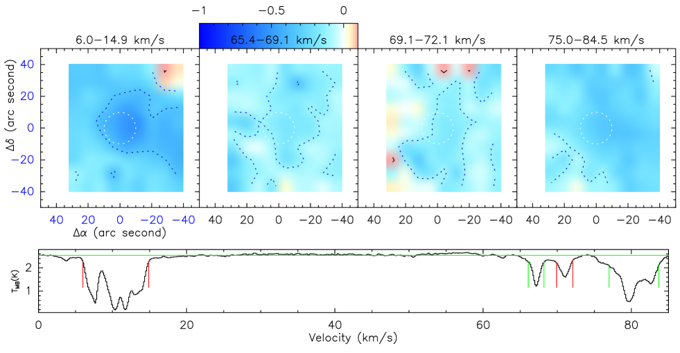
Figure 5: Maps of the p-H₂O 1₁₁-0₀₀ average absorbed fraction ¡$\frac{T-T_{cont}}{T_{cont}}$¿ in four velocity ranges bracketing the main four diffuse line of sight cold clouds. Velocity ranges are given above each box and marked on the low signal to noise spectrum observed at (0,0) by Herpin et al. (2012), the horizontal green line marks the continuum level (K unit). The color scale is clipped in the range [-1,+0.1]. The white dashed circle stands for the beam at 1113 GHz at the (0,0) position. These maps show an almost constant signal over all positions having a detectable continuum level. The MM1 core, located inside the beam circle is barely visible

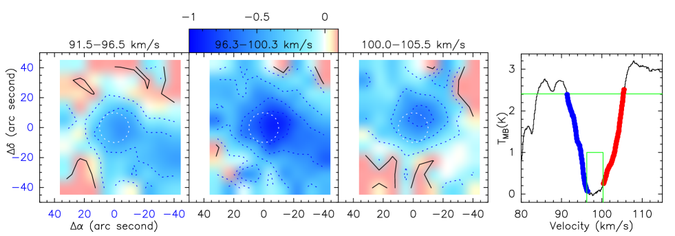
Figure 6: From left to right: maps of the average absorbed fraction ¡$\frac{T-T_{cont}}{T_{cont}}$¿ of the main p-H₂O 1₁₁-0₀₀ line blue wing, center and red wing. Right: The (0,0) spectrum as in Fig. 5 (K units), the blue and red wing ranges are color marked on it. Other plot options are the same as in Fig. 5. These maps show that the blue wing material peaks south-east whereas the red wing peaks north, north-east.

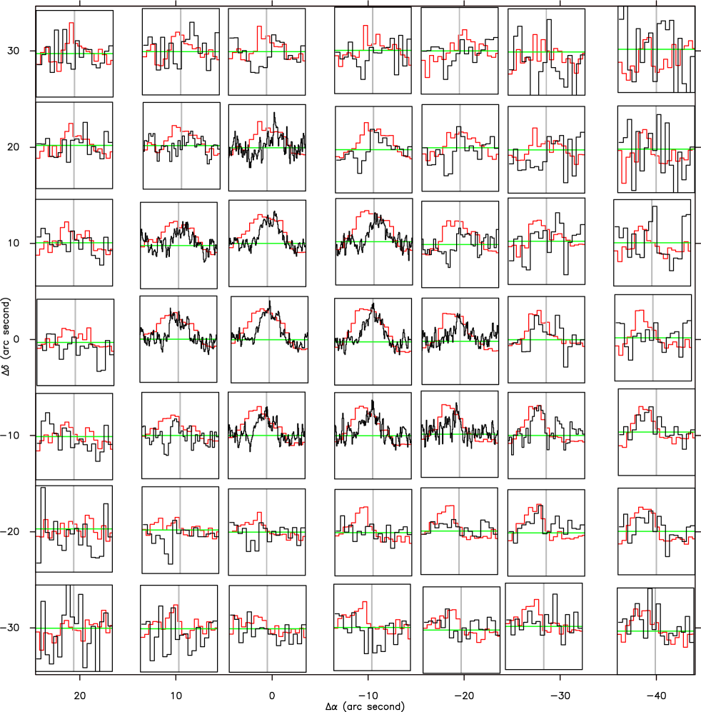
Figure 7: Map toward W43 MM1 of $\frac{T_{cont}-T}{T_{cont}}$ for p-H₂O 1₁₁-0₀₀ (red) and p-H${}_{2}^{18}$O 1₁₁-0₀₀ (black) in the velocity range $[90\,{\rm\ km\ s^{-1}},110\,{\rm\ km\ s^{-1}}$ ]. The Y axis is from -0.1 to 1.1 for p-H₂O 1₁₁-0₀₀ and, p-H${}_{2}^{18}$O 1₁₁-0₀₀ is scaled by 4. The horizontal green lines define the zero level. The vertical grey lines mark $100{\rm\ km\ s^{-1}}$ . As the signal to noise ratio increases for decreasing T_cont, the spectra velocity resolution varies over the map in order to keep it at a minimum value. Hence, with the greatest T_cont, central spectra having a greater number of channels appear plotted darker than those with a lower T_cont. Axis units are offset ($\arcsec$) from MM1.

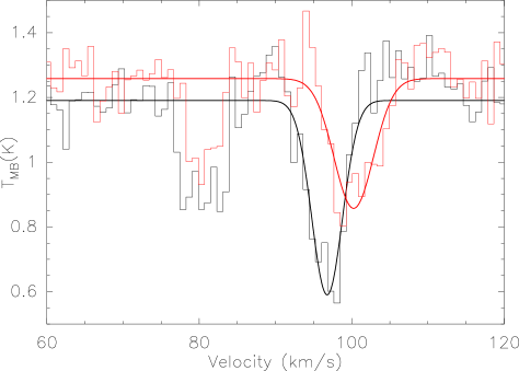
Figure 8: This plot compares p-H₂O 1₁₁-0₀₀ spectra towards our map at offsets around (-18″,-20″) in black and around (+18″,+20″) in red.

3 Mapping result

The observations discussed here map, in three different frequency ranges, a region of about 80″ by 80″ centered on the W43 MM1 core observed, with a very good signal to noise ratio, in Herpin et al. (2012). With a much higher rms per spectrum, our maps still exhibit the same velocity components, in varying proportions over the map: a wide ($\Delta V\simeq 40{\rm\ km\ s^{-1}}$) emission, a narrower ($\Delta V\simeq 10{\rm\ km\ s^{-1}}$) emission, and a rather deep absorption of a continuum background component. Fig. 1-3 show the spectra around MM1 for various velocity ranges bracketing the main water line and also, in Fig. 1 and 3, the highest velocity diffuse line of sight cold cloud (see Herpin et al. 2012). Strongly dominated by the MM1 core, these maps, because of an extended continuum background, still reveal structure far from MM1, making the continuum component a key feature to trace the water lines outside the MM1 core.

The analysis of Herpin et al. (2012) needed a cold water cloud to correctly describe the various water line profiles. Unlike the core, this foreground material might be resolved in these maps which show that, where p-H₂O 2₀₂-1₁₁ is mainly detected around MM1, the lines of p-H₂O 1₁₁-0₀₀ and o-H₂O 1₁₀-1₀₁ are detected at all positions having a positive continuum level. The continuum background (Fig. 4) which peaks at 2.5 K for p-H₂O 1₁₁-0₀₀ at the W43 MM1 core position is almost completely absorbed for channels close to the source velocity. But both blue and red wing of the main absorption showing different behaviours around the core will help to analyze the cold foreground material close to MM1.

Fig. 1 shows the observed spectra towards W43 MM1 for lines p-H₂O 1₁₁-0₀₀ (black), p-H${}_{2}^{18}$O 1₁₁-0₀₀  and ¹³CO (10-9) (inverted to help comparison). These water spectra exhibit a strong absorption against an extended continuum. The HIFI beam does not resolve the MM1 core material, above 100 K, but is small enough to map the continuum region and hence the very close surroundings of MM1.
Fig. 2 shows the observed spectra towards W43 MM1 for lines o-H₂O 1₁₀-1₀₁ , p-H₂O 1₁₁-0₀₀ and o-H${}_{2}^{18}$O 1₁₀-1₀₁. The water spectra are seen in emission and are thus mainly seen toward the MM1 core.
Fig. 3 shows the observed spectra towards W43 MM1 for lines p-H₂O 2₀₂-1₁₁  and C¹⁸O (9-8) (restricted to spectra with a signal to noise ratio good enough). The angular resolution is similar to the map size and help very little to map the MM1 surrounding material.

3.1 Continuum background

Though our spectra do contain continuum, its precise level is somewhat uncertain. We mapped the water lines in W43 MM1 using a fast On-The-Fly mapping HIFI-AOT which allowed to save observing time but at some price. The continuum level variation between two consecutive spectra along the drifts exhibits variations much above these expected from the spectra rms. These variations are especially large at the edges of the region where the continuum level is weaker. One even detects lines in absorption though the continuum level appears negative in the spectrum. Mapping the continuum derived from our maps produces various small artifacts due to these random level variations. The overall structure of the region is correctly reproduced but absolute values of the continuum are unreliable at the smaller scales. As we want to use the continuum level to evaluate the opacity of the absorbing water material, it will produce large errors in parts of the map of low continuum intensity.

To overcome this problem we decided to get an estimate of the true value of the continuum level by using data obtained with SPIRE at $250\text{\,}\mathrm{\SIUnitSymbolMicro m}$ (Nguyen-Lu’o’ng et al. 2013). Our best map for comparison is the p-H₂O 1₁₁-0₀₀ one whose wavelength is $269\text{\,}\mathrm{\SIUnitSymbolMicro m}$ quite close to the SPIRE data. Fig. 4 shows an image of the continuum level observed by SPIRE at $250\text{\,}\mathrm{\SIUnitSymbolMicro m}$ whose angular resolution was smoothed to the p-H₂O 1₁₁-0₀₀ one. The continuum derived from the p-H₂O 1₁₁-0₀₀ spectra observed at 1113 GHz is overplotted as contour levels. The SPIRE map of the continuum has a strong and unresolved peak located at the MM1 position but, at lower levels it follows an underlying aligned north-east to south-west structure anchored to the MM1 position. It decreases rapidly towards the edges of the map along the south-west map axis and more slowly towards the south-east part of the map. The smallest beam size ($\simeq$20″, p-H₂O 1₁₁-0₀₀) does not resolve the 10″central MM1 source but does resolve the extended continuum structure. Thus, having observed absorption lines more than a beam away from MM1 we can get an insight to the material surrounding the central core. Despite level uncertainties in the HIFI map, a comparison of both maps shows a small offset $(-4\arcsec,+2\arcsec)$ between the two peak locations. The reason of this discrepancy is unknown. A map of the region obtained by SCUBA/JCMT at $450\text{\,}\mathrm{\SIUnitSymbolMicro m}$ (Chavarria, priv. comm.) is also available. The SPIRE and SCUBA maps have a highly similar geometry apart from a less than $3\arcsec$ north-south shift between the peaks positions. Part of the data analysis which follows uses, for p-H₂O 1₁₁-0₀₀, the computation of the absorbed fraction $\frac{T-T_{cont}}{T_{cont}}$. The error on this quantity is highly dependent on the $T_{cont}$ value. The low reliability on the p-H₂O 1₁₁-0₀₀ continuum level makes it too difficult to use. Thus, we decided to modify the observed continuum level in all spectra using a model derived from the SPIRE map.

3.2 Model of the continuum background

We build a new set of p-H₂O 1₁₁-0₀₀ spectra by setting the continuum level in each spectrum to a new value derived using the following procedure. We build the continuum model of the region at 1113 GHz from the SPIRE map smoothed at the HIFI p-H₂O 1₁₁-0₀₀ spatial resolution to get the map geometry. We then derive the intensity of the peak from the Herpin et al. (2012) observation. For the latter, one could note that the main absorption in this spectrum goes below zero. This observation was done in a beam switch mode. The SPIRE map showed that the OFF positions were not fully free of continuum, especially the east one. Taking this into account as well as the spectral index between the USB and LSB band and also, the slight offset between this spectrum and the position of the maximum in the map we set the map maximum to 3.71 K. The second step of our continuum building process is to shift the HIFI map by $(-4\arcsec,+2\arcsec)$ in order to correct the observed discrepancy between maps (see above). We think that this step is necessary as without it, in the final map many of the spectra having the deepest absorption will fall below the zero level. Once done, we can easily find for each spectrum the new continuum level value at the corresponding offset in the model.

3.3 Spectral maps

All data exhibit various absorption features between $0{\rm\ km\ s^{-1}}$ and $140{\rm\ km\ s^{-1}}$. At almost all map positions, even further than one p-H₂O 1₁₁-0₀₀ beam size, all water lines, as well as p-H${}_{2}^{18}$O 1₁₁-0₀₀, exhibit an often wide and well defined absorption close to the source velocity. The detection of weaker and narrower absorptions at positions distant from MM1 by much more than a beam size proves that the absorbing material extends over a region bigger than the unresolved MM1 core itself. Many narrower absorptions are also seen at lower velocities ranging from $85{\rm\ km\ s^{-1}}$ down to $0{\rm\ km\ s^{-1}}$. These were interpreted by Herpin et al. (2012) as absorbing material on the line of sight in front of the continuum background, the so-called diffuse line of sight cold clouds. This cold material is thought to be spatially unrelated to MM1 (see Van der Tak et al. 2013).

The three maps discussed in this paper are of unequal interest to investigate the MM1 region structure. o-H₂O 1₁₀-1₀₁ spectra have a good rms but, an angular resolution about four times larger than the source size. The p-H₂O 2₀₂-1₁₁ map contains a few bad spectra for one of the On-The-Fly pass, giving rise to a high signal to noise. p-H₂O 1₁₁-0₀₀, detected in absorption against the extended continuum, with the best rms among the three maps, is thus the most promising line to map the kinematics and physical structure at sizes comparable to the MM1 core. Opacity maps (Fig. 5 and Fig. 6) later derived from these data will help to separate line components over the map.

3.3.1 The main absorption component

At the MM1 position, the three water lines absorption velocity varies between 97.8 and $99.3{\rm\ km\ s^{-1}}$ whereas o-H₂O 1₁₀-1₀₁ and p-H₂O 1₁₁-0₀₀ are seen strongly absorbed at the source velocity. p-H₂O 2₀₂-1₁₁ with a higher energy level is a line whose profile exhibits a well-visible emission component (see central position of Fig.1-3). As one would expect, the deepest p-H₂O 1₁₁-0₀₀ absorption in the map is indeed observed at the location of the strongest continuum component, i.e. the MM1 location.

3.3.2 p-H₂O 1₁₁-0₀₀ map

Fig. 1 shows spectra for p-H₂O 1₁₁-0₀₀, p-H${}_{2}^{18}$O 1₁₁-0₀₀ and ¹³CO (10-9). The ¹³CO (10-9) line is plotted inverted to ease the profile comparisons. The spectral resolution differs for each line. One sees that the p-H${}_{2}^{18}$O 1₁₁-0₀₀ spectra (in red) are narrower than the p-H₂O 1₁₁-0₀₀ spectra and located on the red part of the p-H₂O 1₁₁-0₀₀ line whereas the ¹³CO (10-9) line (in green) appears more blue shifted. One will also note that the diffuse line of sight cold clouds are detected only for p-H₂O 1₁₁-0₀₀ and o-H₂O 1₁₀-1₀₁ as already stated in Herpin et al. (2012).

3.3.3 o-H₂O 1₁₀-1₀₁ map

Fig. 2 shows spectra toward W43 MM1 for o-H₂O 1₁₀-1₀₁ and o-H${}_{2}^{18}$O 1₁₀-1₀₁. The p-H₂O 1₁₁-0₀₀ line spectrum is added for comparison of maps. Despite a $40\arcsec$ beam size comparable to the map size one sees various differences between both lines over the maps.
The diffuse line of sight cold cloud  absorptions are detected in o-H₂O 1₁₀-1₀₁ but not in the o-H${}_{2}^{18}$O 1₁₀-1₀₁ isotopic line, except for the (0″,+35″) position. The diffuse line of sight cold cloud signal evolution correlates strongly over the map with the corresponding signal in the p-H₂O 1₁₁-0₀₀ line.
Both the o-H₂O 1₁₀-1₀₁ line (black spectrum) and the o-H${}_{2}^{18}$O 1₁₀-1₀₁ (red spectrum) line are well detected over all the map. o-H₂O 1₁₀-1₀₁ appears as the merging of a deep absorption and of a wider emission component only seen for the closest spectra to MM1. The absorbing component appears narrower for o-H₂O 1₁₀-1₀₁ than for the p-H₂O 1₁₁-0₀₀ line (green spectrum) at the central position and much more similar on the outer part of the map. The wide emission is brighter than for p-H₂O 1₁₁-0₀₀.
The o-H${}_{2}^{18}$O 1₁₀-1₀₁ main absorption appears narrower than o-H₂O 1₁₀-1₀₁ and is also red-shifted.

3.3.4 p-H₂O 2₀₂-1₁₁ map

Fig. 3 shows spectra for p-H₂O 2₀₂-1₁₁ and C¹⁸O (9-8). This On-The-Fly map was achieved in two passes. In the second one, a few group of spectra suffered from poor baselines making the resulting map inhomogeneous if using the summed spectra or with a too low rms if using only the first pass. Fig. 3 shows the sum of the two passes. C¹⁸O (9-8) spectra being the most impacted by the bad baseline, the central spectrum is the only one shown in Fig. 3. One notes that the C¹⁸O (9-8) line is seen in emission at the velocity of the absorbed p-H₂O 2₀₂-1₁₁ component.

Though the high rms of these spectra makes it difficult to detect too weak p-H₂O 2₀₂-1₁₁ lines, we do detect these lines off the MM1 center. The $21.3\arcsec$ beam size is small enough to allow some mapping off the source core, in particular of the wings. One easily sees the line profile changes around the spectrum at the (0,0) position. The blue wing part of the emission is seen up to the (0″,20″) position whereas the red one has almost disappeared. The red wing is more pronounced south-west of MM1. There is also some reliable signal in the south-east part of the map, see the [-30″,-20″ to 0″] three spectra. One also notes that the red wing is still detected at the west of MM1 whereas the blue one became weaker.

3.4 Absorbed fraction maps

As explained above, variations in the intensities of the absorptions are dominated by the variations of the continuum background. Hence, mapping these intensities does not map water but, mostly reproduce the continuum geometrical structure over the map. However, it is possible to remove this continuum contribution by plotting the absorbed fraction $\frac{T-T_{cont}}{T_{cont}}$ over the mapped region. Fig. 5 and Fig. 6 show the integrated value of the absorbed fraction within some selected velocity range. Foreground clouds detected in absorption were identified in Chavarría et al. (2010) and Herpin et al. (2012) from their velocities. Here we use a different method based on the idea that foreground clouds are necessarily nearer and thus likely to be fairly homogeneous over the small (sub-pc) scales observed in the maps presented in this article. Fig. 5 shows the behaviour of absorbed fraction over the map for the four main diffuse line of sight cold clouds. The MM1 source is within the white dashed circle. One can note that the absorbed fraction is almost constant at all positions following the continuum background. This favors the idea that the signal originates from some foreground material unconnected with MM1 itself.
Fig. 6 plots absorbed fraction for three parts of the main p-H₂O 1₁₁-0₀₀ absorption, namely the blue wing of the line, its central part, and its red wing. One notes here a different behaviour with the diffuse line of sight cold clouds. One only sees the outer part of the MM1 core, the core material itself is shielded. But, one also notes that blue and red wings behave differently as they locate symmetrically around MM1.

Fig. 7 compares absorbed fraction spectra computed for p-H₂O 1₁₁-0₀₀ and p-H${}_{2}^{18}$O 1₁₁-0₀₀. The noise in absorbed fraction spectra increases when $T_{cont}$ decreases making the outer part of the map too noisy. To handle this difficulty we applied a variable spectral resolution to these spectra in order to keep this noise within acceptable values. The spectral resolution decreases with $T_{cont}$, mainly with the distance to MM1. The continuum contribution to the geometry of the map having been subtracted, these spectra present us the spatial variation of the absorbing material. Similar absorbed fraction mean similar opacities. This figure confirms that the blue wing of p-H₂O 1₁₁-0₀₀ has almost no corresponding p-H${}_{2}^{18}$O 1₁₁-0₀₀ counterpart on the contrary to the red one.

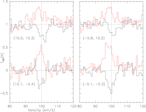
Figure 9: p-H${}_{2}^{18}$O 1₁₁-0₀₀ averaged spectra around the (0,0) position. The average center position is given in ″ offsets below each spectrum. Top spectra were shifted by 1K for plotting purpose. Averaged ¹³CO (10-9) spectra (same positions) are overplotted in red. The continuum is removed for both lines, horizontal grey lines mark the zero levels and, the vertical grey lines mark $100{\rm\ km\ s^{-1}}$.

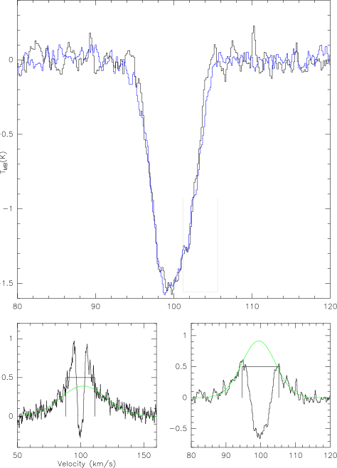
Figure 10: The p-H${}_{2}^{18}$O 1₁₁-0₀₀ absorption versus p-H₂O 2₀₂-1₁₁ (continuum level subtracted) after a wide then narrow Gaussian components removal. The wide component is fitted in the lower left box. The wide removed spectrum is shown in the lower right box with a fit of the narrow component. The upper box shows the final result where the p-H${}_{2}^{18}$O 1₁₁-0₀₀ spectrum intensity is scaled to the absorption level of p-H₂O 1₁₁-0₀₀ . This shows the high similarity of both profiles. Intensities are in K in all boxes.

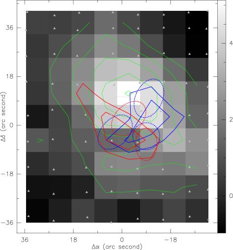
Figure 11: Map of the blue and red wings of the wide p-H₂O 2₀₂-1₁₁ component. Integrated line area are in velocity ranges (${\rm\ km\ s^{-1}}$) : blue=[86,92]; red=[107,117], green=[92,107] (line center, also plotted as grey background). The grey dashed circle at the center gives the beam size. Dashed ellipses mark the position of the three CO (3-2) outflows (OF-1 and OF-2 red TBN) of Fig.2 in Sridharan et al. (2014).

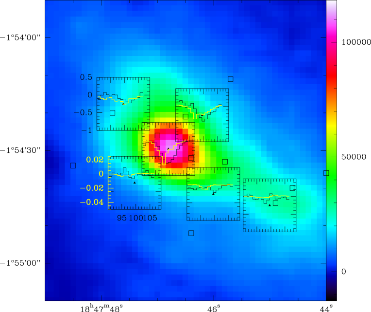
Figure 12: Observed p-H${}_{2}^{18}$O 1₁₁-0₀₀ spectra (black line, temperature scale in black) and predicted p-H${}_{2}^{18}$O 1₁₁-0₀₀ (yellow line, yellow temperature scale) due exclusively to the cool outer material which is believed to be responsible for the H${}_{2}^{16}$O absorption. The zero levels are at the same position but there is a factor 4 difference in the scales, showing clearly that the absorption from the cool material is far from sufficient to explain the observed absorption. Units are ${\rm\ km\ s^{-1}}$ for the velocity and Kelvin for the line temperature. The background is a SCUBA $450\text{\,}\mathrm{\SIUnitSymbolMicro m}$ image with a linear scale and a peak at 110 Jy/beam. The triangles indicate the positions of the spectra. The open squares indicate the Louvet et al 2014 sources.

4 Velocity structure of the W43 core

The comparison of the absorptions of the main H₂O (p-H₂O 1₁₁-0₀₀ and o-H₂O 1₁₀-1₀₁) water lines and of the H${}_{2}^{18}$O (p-H${}_{2}^{18}$O 1₁₁-0₀₀ and o-H${}_{2}^{18}$O 1₁₀-1₀₁) lines (see Fig. 1, Fig. 2, and Fig. 7) shows that, at all the detected positions, the blue side wing of the main water line has no H${}_{2}^{18}$O counterpart. Hence, we think that this blue side of the main water absorption is due to a cold foreground material, possibly surrounding the MM1 core. Though an outflow absorption is partly taken into account in the models in Section 6.2, we cannot rule out a low density outflow as the source of this absorption. Fig. 6 also shows that the redshifted material is located at the immediate north-east off the MM1 core and that the blueshifted material is located south-west of MM1. The central and deepest part of the absorption covers both regions. Though the H${}_{2}^{18}$O absorption probably comes from the inner region of the source, it is also seen off core towards the south-west MM1 following the extended continuum emission.

4.1 Central velocity gradient

Due to its lower optical depths, p-H${}_{2}^{18}$O 1₁₁-0₀₀  traces the inner material whereas the main isotope is optically thick in the surrounding cool gas, such that it does not trace the inner material. Figures 8 and 9 show respectively the main isotope and the p-H${}_{2}^{18}$O 1₁₁-0₀₀ ground state absorption lines at selected positions around MM1. Figure 8 compares the velocity profiles of p-H₂O 1₁₁-0₀₀ spectra between two positions, chosen symmetrically relative to MM1 and separated by more than a full beamwidth, to the SW and NE of MM1. These positions were chosen to be along the extended continuum object, far enough not to detect the emission from the central source but in a region where the absorption is still clearly detected. It is immediately apparent that the W43 MM1 absorption shows a velocity gradient whereas the diffuse line of sight cold cloud at $80\,{\rm\ km\ s^{-1}}$ does not. The diffuse line of sight cold clouds absorptions are rather identical in absorbed fraction where the main absorption shows a kind of complementary profiles. The blue wing is in emission for one position and in absorption for the other one. The opposite behaviour is seen for the red wing. This inversion occurs, in velocity, symmetrically to the $\simeq 99{\rm\ km\ s^{-1}}$ source velocity.

The p-H${}_{2}^{18}$O 1₁₁-0₀₀ is not detectable as far out but Fig. 9 shows a similar velocity gradient in the same direction as for the envelope. It shows four p-H${}_{2}^{18}$O 1₁₁-0₀₀ spectra at positions surrounding MM1 revealing a velocity gradient in the p-H${}_{2}^{18}$O 1₁₁-0₀₀ ranging from $\simeq 98{\rm\ km\ s^{-1}}$ in the south-west of MM1 to $\simeq 102{\rm\ km\ s^{-1}}$ in the north-east part of the MM1 core. The vertical line at the central velocity makes it clear that there is a SW-NE gradient but not SE-NW.

The ¹³CO (10-9)  emission line (Fig. 1, Fig. 9), whose energy is above $200\,{\rm\,K}$, comes from the warm central regions. It has the same gradient but the p-H${}_{2}^{18}$O 1₁₁-0₀₀ absorption is consistently redshifted with respect to the ¹³CO (10-9), showing that the infall onto the main source is visible throughout the inner region. As for the p-H${}_{2}^{18}$O 1₁₁-0₀₀ line, the ¹³CO (10-9) line velocity shift of $0.7{\rm\ km\ s^{-1}}$ is seen from south-west (offset -8″,-8″) to north-east (offset +8″,+8″), going from 97.9 to $98.6{\rm\ km\ s^{-1}}$. While the size of our beam and the signal-to-noise level of the observations does not allow us to measure the size of the region from which ¹³CO (10-9) emission is detected, the shift shows that it is not point-like even to our $20\,\arcsec$ beam. The small velocity shift shows that the core is not rotationally supported, in agreement with the presence of the infall signature.

4.2 p-H${}_{2}^{18}$O 1₁₁-0₀₀ versus p-H₂O 2₀₂-1₁₁

Figure 10 compares the p-H${}_{2}^{18}$O 1₁₁-0₀₀ profile to the p-H₂O 2₀₂-1₁₁ absorption profile at the MM1 position. We first fit a Gaussian profile to model the wide component (see lower left spectrum in figure). Once done, we removed it from the spectrum. Then, we fit the emission part of the remaining spectrum by another Gaussian profile (see lower right spectrum in figure) that we again remove. The hypothesis here is that both the wide and the narrower emission parts of the line profile can be modeled by Gaussian profiles. The last spectrum fits then the absorbing component in the p-H${}_{2}^{18}$O 1₁₁-0₀₀ line. We compare its profile to the p-H₂O 2₀₂-1₁₁line by scaling both lines to the same intensities (see upper box in figure). Both profiles are almost identical in width. The little dip in the red wing is even the same in the two spectra. We conclude that both lines originate from the same material.

4.3 The wide component high-velocity gas

A wide velocity component is observed in several main water lines (see Herpin et al. 2012). We detect it in our maps of o-H₂O 1₁₀-1₀₁ , p-H₂O 2₀₂-1₁₁ and p-H₂O 1₁₁-0₀₀. The wide component in the o-H₂O 1₁₀-1₀₁ map is detected at all observed positions but not used in our discussion because of the large beam size at 557 GHz. Because of a poor rms and of some baseline problems there are large uncertainties for the p-H₂O 2₀₂-1₁₁ spectra. Still, it is possible to map the wide $\simeq 40{\rm\ km\ s^{-1}}$ component wings of p-H₂O 2₀₂-1₁₁ as seen in Fig. 11 where one sees the red and blue wings bracketing the central absorption in the southern part of MM1.
We searched for traces of systematic motion in the high-velocity gas seen in p-H${}_{2}^{18}$O 1₁₁-0₀₀ emission. Fig. 11 shows the spatial distribution of the line emission, with red-shifted gas in red, blue-shifted gas in blue, and intermediate velocity gas in green. The quiescent gas is seen to trace a flattened envelope which is also seen in the continuum (Fig. 4), while the high-velocity gas is seen to trace two lobes which fall on a line which is approximately perpendicular to this envelope. If these lobes are due to a bipolar outflow, Fig. 11 indicates a size of $\sim$36” end-to-end or $\sim$18” peak-to-peak, which at 5.5 kpc (Zhang et al. 2014) corresponds to 0.48-0.96 pc. While the map data in Fig. 11 indicate a velocity range of only $\sim 31{\rm\ km\ s^{-1}}$ FWZI or $\sim 25{\rm\ km\ s^{-1}}$ FWHM for the outflow, the pointed spectrum in Fig. 10 shows that p-H${}_{2}^{18}$O 1₁₁-0₀₀  emission is detected at higher velocities, up to $\sim 50{\rm\ km\ s^{-1}}$ FWZI. Furthermore, Fig. 11 indicates a low degree of collimation for the outflowing gas, as often seen in single-dish observations of outflows from massive star-forming regions (Beuther & Shepherd 2005).

Outflow activity from W43-MM1 has been observed before by Sridharan et al. (2014), who used the SMA to image the CO 3-2 line emission from this region at 5” resolution. Their data reveal gas shifted to velocities up to $\sim 70{\rm\ km\ s^{-1}}$, which is spatially resolved into 3 distinct bipolar outflows, which together cover an area of 20-30” in size. Thus, our observed high-velocity p-H${}_{2}^{18}$O 1₁₁-0₀₀ emission may trace dense gas associated with the high-velocity CO seen with the SMA, and the apparent low collimation may be due to confusion between multiple bipolar outflows.

5 Envelope absorption and velocity gradient

Figure 7 points to the same effect: the blue wing is seen in absorption to the SW and the red wing to the NE. The total velocity shift is around 4 to 5 ${\rm\ km\ s^{-1}}$

A major question is how one can directly observe the massive protostellar core. It appears that the main isotope p-H₂O 1₁₁-0₀₀  absorption at 1113 GHz comes from the envelope rather than the region above 100 K (Herpin et al. 2012). In order to assess whether the p-H${}_{2}^{18}$O 1₁₁-0₀₀ absorption is due to the cool envelope or the protostellar core, we used the line to continuum ratio of the p-H₂O 1₁₁-0₀₀  line to estimate the optical depth at 1113 GHz, implicitly assuming that all of the absorption is due to the envelope. With a minor calibration error, one could easily underestimate or overestimate the p-H₂O 1₁₁-0₀₀ optical depth. If the absorption were underestimated, one would expect to have extreme variations in the optical depth as e.g. a 99.99% absorption will yield a much higher optical depth than 99% absorption and the variations due to noise are at this level. If we have overestimated the absorption, then the p-H${}_{2}^{18}$O 1₁₁-0₀₀ absorption will also be overestimated. The absorption is shown in Fig. 6, where the highest contour is at an absorption level of 78% over a width of $4{\rm\ km\ s^{-1}}$, consistent with the somewhat higher absorptions we obtain for the $2{\rm\ km\ s^{-1}}$ width used in these calculations. Then, assuming an abundance ratio H₂O/H${}_{2}^{18}$O of 322, corresponding to the galactocentric radius of W43 (Wilson & Rood 1994), we calculate the optical depth and (using the continuum flux) expected absorption line intensity. This can be directly compared to the observed p-H${}_{2}^{18}$O 1₁₁-0₀₀ absorption spectra.

Figure 12 shows the observed p-H${}_{2}^{18}$O 1₁₁-0₀₀ absorption and predicted p-H${}_{2}^{18}$O 1₁₁-0₀₀ envelope absorption spectra superposed on a SCUBA $450\text{\,}\mathrm{\SIUnitSymbolMicro m}$ map. It can be seen that while there is p-H${}_{2}^{18}$O 1₁₁-0₀₀ absorption associated with the envelope, the expected line intensity is below 0.04 K everywhere. The observed p-H${}_{2}^{18}$O 1₁₁-0₀₀ absorption reaches 1 K in the central regions, incompatible with the hypothesis that the p-H${}_{2}^{18}$O 1₁₁-0₀₀ absorption is due to the envelope. In both the predicted envelope spectra and observed spectra, p-H${}_{2}^{18}$O 1₁₁-0₀₀ lines are predicted/detected in regions along the major axis of W43 MM1.

Therefore, the p-H${}_{2}^{18}$O 1₁₁-0₀₀  absorption is due to the central core region which has $T_{mb}>100{\rm\,K}$. As also shown in Figure 7, the velocities of the p-H₂O 1₁₁-0₀₀ and p-H${}_{2}^{18}$O 1₁₁-0₀₀ lines are not the same, further illustrating that they trace different components. The ¹³CO (10-9) emission (Fig. 1), tracing warm dense material and observed at the same positions with exactly the same beam size, is systematically at a less redshifted velocity than the p-H${}_{2}^{18}$O 1₁₁-0₀₀  implying that the water over 100 K is infalling.

Figure 5 and Fig. 6 visualize the absorbed fraction, for various velocity ranges, of the p-H₂O 1₁₁-0₀₀ line. The situation in Fig. 6 is clearly different compared to Fig. 5. The diffuse line of sight cold cloud mapped in Fig. 5 do not show the same localized structure seen in Fig. 6. The three upper panels of Fig. 6 show respectively the blue wing, the central part where the absorption is generally higher, and the red wing. There is little absorption to the NE in the blue wing and to the SW in the red, showing a velocity gradient in the envelope.

p-H${}_{2}^{18}$O 1₁₁-0₀₀ emission/absorption is also present outside the central beam. We believe that this is due to the other massive dense cores found by Louvet et al. in W43 MM1. Their positions are indicated on Figure 12 and this can be compared with the p-H${}_{2}^{18}$O 1₁₁-0₀₀ optical depth as seen in Figure 7, showing the same result in a slightly different manner.

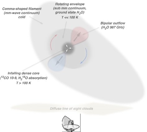
Figure 13: Drawing of the various W43 MM1 components derived from the spectral maps. Arrows sketch the corresponding velocity fields (infall, outflow and rotation). The observing direction is indicated by the bottom telescope image whose dimension give an idea of the beam size.

6 Source structure and Infall rate

Based on results of the previous sections, Fig. 13 sketches out the kinematics and physical structure of W43 MM1, sizes and geometry of the various components are roughly indicative. The extended comma shape continuum component contains the infalling W43 MM1 core embedded in a colder envelope. The saturated p-H₂O 1₁₁-0₀₀ water line comes from the colder envelope whereas p-H${}_{2}^{18}$O 1₁₁-0₀₀ and ¹³CO (10-9) come from the hotter infalling core. The envelope component is resolved by the Herschel beam at $1113\,GHz$. Its possible rotation is suggested by the water lines velocity gradient seen around the core along the comma shape axis. This sketch does not show the many cores sub structure seen in Louvet et al. (2014) and, gives only the global orientation of the outflow seen in p-H₂O 2₀₂-1₁₁.

6.1 The cold foreground material

As explained in Sect. 4 and Fig. 7, a cold foreground cloud embedding MM1 contributes to the blue side of the line profile of the para ground state line of water. We modeled this blending component using our map data as follows. Figure 5 (see left box) shows that the opacity of this material can, at first, be considered rather constant in between MM1 and the south-west part of the map allowing us to make the raw hypothesis that the physical conditions of this material are similar enough both at MM1 and at a location around the offset (-21″,-14″). We fit the line at this off core position and, we then scale this result using the continuum ratio at MM1 and at the off core position in order to remove it from the spectrum observed towards MM1. Subtracting this absorption from the pointed spectra of MM1 from Herpin et al. (2012), we get an estimate of the true water line profile toward the massive dense core MM1 (see Fig. 14). The new line profile is of course narrower and the absorption less deep, now rather peaking at $100{\rm\ km\ s^{-1}}$, i.e. red-shifted relative to the source velocity.

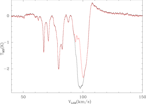
Figure 14: Original HIFI spectra of the p-H₂O 1₁₁-0₀₀line in black (from Herpin et al. (2012)). In red the spectra after removing of the cold component.

This blue side cold component is also seen in the ortho ground state lines o-H₂O 1₁₀-1₀₁ and o-H₂O 2₁₂-1₀₁. Unfortunately, missing the corresponding H₂O line maps, we cannot apply the method described above for the p-H₂O 1₁₁-0₀₀ line profile. Still, we can get an estimate of this blue side blending by comparing the many diffuse line of sight cold clouds components seen in o-H₂O 1₁₀-1₀₁ and o-H₂O 2₁₂-1₀₁ between 0 and 90 ${\rm\ km\ s^{-1}}$ to their p-H₂O 1₁₁-0₀₀ counterparts. We note that their integrated intensity (for both o-H₂O 1₁₀-1₀₁ and o-H₂O 2₁₂-1₀₁) can be scaled with almost the same value at all velocities from each p-H₂O 1₁₁-0₀₀ counterpart. From our hypothesis that the p-H₂O 1₁₁-0₀₀ blue side material has a diffuse line of sight cold cloud nature we can then model it for the o-H₂O 1₁₀-1₀₁ and o-H₂O 2₁₂-1₀₁ main water line by scaling our fit for p-H₂O 1₁₁-0₀₀ with the scale ratio found for the o-H₂O 1₁₀-1₀₁ and o-H₂O 2₁₂-1₀₁”cold” components. We can now derive the corrected o-H₂O 1₁₀-1₀₁ and o-H₂O 2₁₂-1₀₁ water line profiles (see Fig. 15).

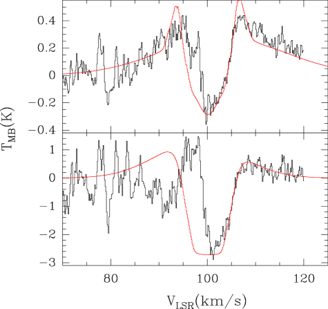
Figure 15: HIFI spectra after removing of the cold component for the 557 (top) and 1669 GHz (bottom) lines. In red is shown the new model.

6.2 The warm protostellar envelope

Considering that these new line profiles give us a more realistic view of the MM1 source, we decide to revisit the analysis of Herpin et al. (2012) who needed a cold water cloud to properly model the various line profiles. We use the same physical structure for the W43 MM1 source and first apply the same model (same foreground clouds, turbulent velocity, infall and water abundances) than Herpin et al. (2012). Fig. 16 shows that the line profile is not well reproduced: the modeled spectra is too broad and exhibits a saturated deep absorption. The best model is obtained by only decreasing the global outer water abundance from 8 $10^{-8}$ to 8 $10^{-9}$; the inner water abundance and the turbulence velocity increasing with radius have not changed. Surprisingly, a weaker cold component (with an opacity of 0.3) is still needed to reach the absorption dip. The same conclusions apply to the o-H₂O 1₁₀-1₀₁ and o-H₂O 2₁₂-1₀₁ lines (opacity of 0.4 for the cold component) (see Fig. 15).

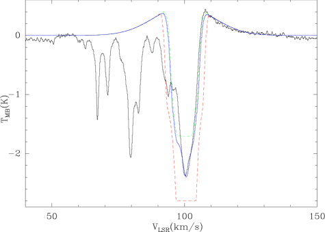
Figure 16: New HIFI spectra of the p-H₂O 1₁₁-0₀₀line in black (from Herpin et al. (2012). The outputs from the model with Herpin et al. (2012) parameters, new parameters without, and with a foreground cloud are respectively shown in red, green, and blue.

Though the outer water abundance in other mid-IR quiet high-mass protostellar objects (HMPO) has been found by Herpin et al. (2016), and also by Marseille et al. (2010), to be of a few $10^{-8}$ (but $1.4\times 10^{-7}$ for DR21(OH)), other estimates in some more evolved massive objects lead to lower values: $2.4-6.3\times 10^{-9}$ in AFGL2591 (Choi et al. 2015) and $1-5\times 10^{-9}$ for some bright HMPOs, hot molecular cores, and Ultra Compact HII regions Choi (2015). In addition, low-mass protostellar objects tend to have an outer abundance of $\sim 10^{-8}$ (Van Dishoeck et al. 2011) or even lower ($3\times 10^{-10}$, Mottram et al. 2013). Moreover, Snell et al. (2000) or Caselli et al. (2012) have estimated very low abundances ($10^{-10}-10^{-8}$) in cold regions. Hence the value derived in our study is compatible with what is found in cold outer regions. In the cold envelopes, water is mainly found as ice and can sublimate through FUV photodesorption (photons from the interstellar radiation field, ISRF, and from cosmic rays interacting with H₂, see Schmalzl et al. 2014). Of course, part of this water vapour can then be photodissociated through FUV photons. Variations of the ISRF (e.g. proximity of a nearby bright star) or self-shielding for instance can lead to different outer abundances for different objects.

While we find lower outer water abundances than derived from pointed observations, it is unlikely that this can be generalized to other sources. W43 MM1 is indeed part of a complex cluster embedded in an elongated structure (Louvet et al. 2014). Only further studies of similar maps observed toward these objects can help to confirm or revise previous water abundances.

In the new models, as for ${\rm NH}_{3}\ 3_{2+}\,-\,2_{2-}$ in Wyrowski et al. (2012), the lines are now centered at $100{\rm\ km\ s^{-1}}$ rather than $98.6{\rm\ km\ s^{-1}}$ before in Herpin et al. (2012), hence red-shifted relative to the source velocity, which is indicative of infall. While in Herpin et al. (2012), the ground-state lines were dominated by the cold cloud (in absorption), and thus were not showing any infall signature, these new water line profiles do indicate infall. This infall signature is now well reproduced by this new model using the same infall velocity ($-2.9{\rm\ km\ s^{-1}}$) than Herpin et al. (2012), then mainly derived from the 987 and 752 GHz water lines. Before subtraction of the widespread cool component, the low-energy H₂O lines were not sensitive to infall, which could only be traced at higher energies and/or with isotopologues. Now the H₂O lines yield the same level of infall. The main consequence of this new outer water abundance is that the water content in the outer region is an order of magnitude lower than previously estimated: 3.7 $10^{-4}$ M_⊙ (instead of 3 $10^{-3}$ M_⊙).

7 Conclusions

The main conclusion from this work is that map data are an essential complement to pointed observations to ensure reliable estimation of physical and chemical parameters from sub-millimeter line spectra. In particular, molecular abundances derived only from pointed spectra may be off by a factor of $\simeq 10$, while estimates of turbulent velocities and infall / outflow rates are less affected.

Our second conclusion is that lines of H${}_{2}^{18}$O, as well as excited-state H₂O lines, trace the inner envelopes of high-mass protostars, where abundances are enhanced due to grain mantle evaporation and/or high-temperature gas-phase chemistry. Deriving these abundances requires careful subtraction of the contribution from the outer envelope, however.

Third, we find that warm chemically enriched gas in W43 is not confined to the MM1 position, but is also found towards other cores seen in warm dust emission by Louvet et al. (2014).

Finally, the HIFI maps of the W43 region reveal velocity gradients in the envelope of the MM1 core as well as in the surrounding gas, which are indicative of rotation. Figure 13 summarizes the global picture derived for the MM1 region.

References

- Beuther et al. (2007) Beuther, H., Churchwell, E. B., McKee, C. F., & Tan, J. C. 2007, Protostars and Planets V, 165
- Beuther & Shepherd (2005) Beuther, H. & Shepherd, D. 2005, in Cores to Clusters: Star Formation with Next Generation Telescopes, ed. M. S. N. Kumar, M. Tafalla, & P. Caselli, 105–119
- Caselli et al. (2012) Caselli, P., Keto, E., Bergin, E. A., et al. 2012, ApJ, 759, L37
- Chavarría et al. (2010) Chavarría, L., Herpin, F., Jacq, T., et al. 2010, A&A, 521, L37
- Choi (2015) Choi, Y. 2015, PhD thesis, Groningen
- Choi et al. (2015) Choi, Y., van der Tak, F. F. S., van Dishoeck, E. F., Herpin, F., & Wyrowski, F. 2015, A&A, 576, A85
- de Graauw et al. (2010) de Graauw, T., Helmich, F. P., Phillips, T. G., et al. 2010, A&A, 518, L6
- Herpin et al. (2016) Herpin, F., Chavarría, L., Jacq, T., et al. 2016, A&A, 587, A139
- Herpin et al. (2012) Herpin, F., Chavarría, L., van der Tak, F., et al. 2012, A&A, 542, A76
- Louvet et al. (2014) Louvet, F., Motte, F., Hennebelle, P., et al. 2014, A&A, 570, A15
- Marseille et al. (2010) Marseille, M. G., van der Tak, F. F. S., Herpin, F., et al. 2010, A&A, 521, L32+
- Motte et al. (2003) Motte, F., Schilke, P., & Lis, D. C. 2003, ApJ, 582, 277
- Mottram et al. (2013) Mottram, J. C., van Dishoeck, E. F., Schmalzl, M., et al. 2013, A&A, 558, A126
- Nguyen-Lu’o’ng et al. (2013) Nguyen-Lu’o’ng, Q., Motte, F., Carlhoff, P., et al. 2013, ApJ, 775, 88
- Ott (2010) Ott, S. 2010, in Astronomical Society of the Pacific Conference Series, Vol. 434, Astronomical Data Analysis Software and Systems XIX, ed. Y. Mizumoto, K.-I. Morita, & M. Ohishi, 139
- Pearson et al. (1991) Pearson, J. C., De Lucia, F. C., Anderson, T., Herbst, E., & Helminger, P. 1991, ApJ, 379, L41
- Pilbratt et al. (2010) Pilbratt, G. L., Riedinger, J. R., Passvogel, T., et al. 2010, A&A, 518, L1
- Roelfsema et al. (2012) Roelfsema, P. R., Helmich, F. P., Teyssier, D., et al. 2012, A&A, 537, A17
- Schmalzl et al. (2014) Schmalzl, M., Visser, R., Walsh, C., et al. 2014, A&A, 572, A81
- Snell et al. (2000) Snell, R. L., Howe, J. E., Ashby, M. L. N., et al. 2000, ApJ, 539, L101
- Sridharan et al. (2014) Sridharan, T. K., Rao, R., Qiu, K., et al. 2014, ApJ, 783, L31
- Tan et al. (2014) Tan, J. C., Beltrán, M. T., Caselli, P., et al. 2014, Protostars and Planets VI, 149
- Van der Tak et al. (2013) Van der Tak, F. F. S., Chavarría, L., Herpin, F., et al. 2013, A&A, 554, A83
- Van der Tak et al. (2010) Van der Tak, F. F. S., Marseille, M. G., Herpin, F., et al. 2010, A&A, 518, L107
- Van Dishoeck et al. (2013) Van Dishoeck, E. F., Herbst, E., & Neufeld, D. A. 2013, Chemical Reviews, 113, 9043
- Van Dishoeck et al. (2011) Van Dishoeck, E. F., Kristensen, L. E., Benz, A. O., et al. 2011, PASP, 123, 138
- Wilson & Rood (1994) Wilson, T. L. & Rood, R. 1994, ARA&A, 32, 191
- Wyrowski et al. (2012) Wyrowski, F., Güsten, R., Menten, K. M., Wiesemeyer, H., & Klein, B. 2012, A&A, 542, L15
- Zhang et al. (2014) Zhang, B., Moscadelli, L., Sato, M., et al. 2014, ApJ, 781, 89
- Zinnecker & Yorke (2007) Zinnecker, H. & Yorke, H. W. 2007, ARA&A, 45, 481