Projective Wonderful Models for Toric Arrangements

Abstract

In this paper we illustrate an algorithmic procedure which allows to build projective wonderful models for the complement of a toric arrangement in a $n$-dimensional algebraic torus $T$. The main step of the construction, inspired by [9], is a combinatorial algorithm that produces a toric variety by subdividing in a suitable way a given smooth fan.

1 Introduction

Let us consider a $n$-dimensional algebraic torus $T$ over the complex numbers. Let $X^{*}(T)$ denote its character group. This is a lattice of rank $n$ and choosing a basis of $X^{*}(T)$ we get an isomorphism $T\simeq({\mathbb{C}}^{*})^{n}$.

If we take a split direct summand $\Gamma\subset X^{*}(T)$ and a homomorphism $\phi:\Gamma\to\mathbb{C}^{*}$, we can consider the subvariety, which will be called a layer, in $T$

$$\mathcal{K}_{\Gamma,\phi}=\{t\in T|\,\chi(t)=\phi(\chi),\,\forall\chi\in\Gamma\}.$$

Notice that a layer is a coset for the subtorus $H=\cap_{\chi\in\Gamma}Ker(\chi)$. So it is itself isomorphic to a torus and in particular it is smooth and irreducible.

A toric arrangement ${\mathcal{A}}$ is given by finite set of layers ${\mathcal{A}}=\{\mathcal{K}_{1},...,\mathcal{K}_{m}\}$ in $T$. We will say that a toric arrangement ${\mathcal{A}}$ is divisorial if for every $i=1,...,m$ the layer $\mathcal{K}_{i}$ has codimension 1.

In this paper we show how to construct a projective wonderful model for the complement ${\mathcal{M}}({\mathcal{A}})=T-\bigcup_{i}\mathcal{K}_{i}$, i.e. a smooth projective variety $\mathcal{W}({\mathcal{A}})$ containing ${\mathcal{M}}({\mathcal{A}})$ as an open set and such that $\mathcal{W}({\mathcal{A}})-{\mathcal{M}}({\mathcal{A}})$ is a divisor with normal crossings and smooth irreducible components.

Let us first shortly recall the state of the art about toric arrangements. The study of toric arrangements started in [28]. In the case of a divisorial arrangement, it received a new impulse from several recent works for instance, in [14] and [13] the role of toric arrangements as a link between partition functions and box splines is pointed out; interesting enumerative and combinatorial aspects have been investigated via the Tutte polynomial and arithmetics matroids in [30], [31], [5]. As for the topology of the complement of a divisorial toric arrangement, the generators of the cohomology modules over ${\mathbb{C}}$ where exhibited in [12] via local no broken circuits sets, and in the same paper the cohomology ring structure was determined in the case of totally unimodular arrangements. A presentation of the fundamental group of the complement of a divisorial complexified toric arrangement was provided in [6], and in [7] d’Antonio and Delucchi proved that ${\mathcal{M}}({\mathcal{A}})$ has the homotopy type of a minimal CW-complex and that its integer cohomology is torsion free.

Moreover, in [1] Callegaro and Delucchi computed the cohomology ring with integer coefficients of ${\mathcal{M}}({\mathcal{A}})$ and started to investigate its dependency from the combinatorial data of the arrangement.

The problem of finding a wonderful model for ${\mathcal{M}}({\mathcal{A}})$ was first studied by Moci in [32], where a construction of a non projective model was described.

To explain the interest in the construction of a projective wonderful model, we briefly recall some results in the case of subspace arrangements.

In [10], [11], De Concini and Procesi constructed wonderful models for the complement of a subspace arrangement in a vector space (providing both a projective and a non projective version of the construction), as an approach to Drinfeld construction of special solutions for Khniznik-Zamolodchikov equation (see [16]). Then real and complex De Concini-Procesi models of subspace arrangements were investigated from several points of view: their cohomology was studied for instance in [35], [18], [33]; some relevant combinatorial properties and their relation with discrete geometry were pointed out in [19], [24], [23], [2]; the case of complex reflection groups was dealt with in [25] from the representation theoretic point of view and in [3] from the homotopical point of view; relations with toric and tropical geometry were enlightened for instance in [20] and [15].

Furthermore, we recall that in [11] it was shown, using the cohomology description of the projective wonderful models to give an explicit presentation of a Morgan algebra, that the mixed Hodge numbers and the rational homotopy type of the complement of a complex subspace arrangement depend only on the intersection lattice (viewed as a ranked poset).

By analogy with the linear case, one of the reasons for the interest in the construction of a projective wonderful model for ${\mathcal{M}}({\mathcal{A}})$ is the computation of the Morgan algebra associated to the model and the investigation of its role in the study of the dependency of the cohomology ring of ${\mathcal{M}}({\mathcal{A}})$ from the initial combinatorial data. We leave this as a future direction of research.

Let us now describe more in detail the content of the present paper.

In Section 2 we are going to briefly recall the construction of wonderful models of varieties with a conical stratification in the sense of MacPherson-Procesi [29], or, in other words containing an arrangement of subvarieties in the sense of Li [27].

In Section 3, given a smooth fan $\Delta$ in the vector space $hom_{\mathbb{Z}}(X^{*}(T),{\mathbb{R}})=hom_{\mathbb{Z}}(X^{*}(T),{\mathbb{Z}})\otimes_{{\mathbb{Z}}}{\mathbb{R}}$ and a layer $\mathcal{K}_{\Gamma,\phi}$, we are going to give a simple combinatorial condition which allows us to explicitly describe the closure $\overline{\mathcal{K}}_{\Gamma,\phi}$ in the toric variety $K_{\Delta}$ corresponding to $\Delta$ and the intersection of $\overline{\mathcal{K}}_{\Gamma,\phi}$ with every $T$-orbit closure in $K_{\Delta}$.

Then, given a toric arrangement ${\mathcal{A}}$ in $T$ we will construct a projective wonderful model for the complement ${\mathcal{M}}({\mathcal{A}})$ according to the following strategy:

1. As a first step, we construct (see Sections 4 and 6) a smooth projective $T$-variety $K_{\Delta({\mathcal{A}})}$ (where $\Delta({\mathcal{A}})$ denotes its fan).

   The crucial property of the toric variety $K_{\Delta({\mathcal{A}})}$ is the following one. Let us denote by ${\mathcal{Q}}$ the set whose elements are the closures ${\overline{\mathcal{K}}_{i}}$ of our layers and the irreducible components $D_{\alpha}$ of $K_{\Delta({\mathcal{A}})}-T$. Then the family ${\mathcal{L}}$ of all the connected components of intersections of elements of ${\mathcal{Q}}$ gives an arrangement of subvarieties in the sense of Li’s paper [27], as we will show by a precise description of the closure in $K_{\Delta({\mathcal{A}})}$ of every subvariety in ${\mathcal{L}}$ .

2. As a consequence of point $1)$, for every choice of a building set associated to the arrangement of subvarieties in $K_{\Delta({\mathcal{A}})}$ one can obtain a projective wonderful model of ${\mathcal{M}}({\mathcal{A}})$.

The construction of the toric variety $K_{\Delta({\mathcal{A}})}$ is the result of a combinatorial algorithm on fans that starts from the fan of $({\mathbb{P}}^{1})^{n}$. This algorithm, which is a variant of an algorithm introduced in [9] for a different purpose, is described in Section 4 and illustrated by some examples in Section 5.

In Section 7 we prove that the family of subvarieties ${\mathcal{L}}$ in $K_{\Delta({\mathcal{A}})}$ is an arrangement of subvarieties. The last section (Section 8) is devoted to some remarks on our construction. First we show that, although our construction is not canonical (it depends for instance from the initial identification of the fan of $({\mathbb{P}}^{1})^{n}$), in some cases there is also a more canonical way to obtain a toric variety $K_{\Delta({\mathcal{A}})}$ with the requested properties. This happens for instance for divisorial toric arrangements ${\mathcal{A}}$ associated to root systems or to a directed graph.

Finally we show that if $\mathcal{W}({\mathcal{A}})$ is a projective wonderful model obtained by our construction, then its integer cohomology is even and torsion free and the cohomology ring is isomorphic to the Chow ring (i.e. $\mathcal{W}({\mathcal{A}})$ has property $(S)$ according to the definition in [8] 1.7). This follows from the description of the strata in Section 3 and from the fact that the construction of wonderful models in [29], [27] can be seen as the result of a prescribed sequence of blowups.

2 Wonderful models of stratified varieties

In the literature one can find several general constructions that, starting from a ‘good’ stratified variety, produce models by blowing up a suitable subset of strata. For instance, as we mentioned in the Introduction, the case of the stratification induced in a vector space by a subspace arrangement is discussed in [10], [11].

The papers of MacPherson and Procesi [29] and Li [27] extend the construction of wonderful models from the linear case to the more general setting of a variety stratified by a set of subvarieties.

In Li’s paper one can also find a comparison among several constructions of models, including the ones by Fulton-Machperson ([22]), Ulyanov ([34]) and Hu ([26]). Denham’s paper [15] provides a further interesting survey including tropical compactifications.

We recall here some definitions and results from [29] and [27] adopting the language and the notation of Li’s paper.

Definition 2.1.

A simple arrangement of subvarieties of a nonsingular variety $Y$ is a finite set $\Lambda=\{\Lambda_{i}\}$ of nonsingular closed connected subvarieties $\Lambda_{i}$, properly contained in $Y$, that satisfy the following conditions:
(i) $\Lambda_{i}$ and $\Lambda_{j}$ intersect cleanly, i.e. their intersection is nonsingular and for every $y\in\Lambda_{i}\cap\Lambda_{j}$ we have

$$T_{\Lambda_{i}\cap\Lambda_{j},y}=T_{\Lambda_{i},y}\cap T_{\Lambda_{j},y}$$

(ii) $\Lambda_{i}\cap\Lambda_{j}$ either belongs to $\Lambda$ or is empty.

Definition 2.2.

Let $\Lambda$ be a simple arrangement of subvarieties of $Y$. A subset ${\mathcal{G}}\subseteq\Lambda$ is called a building set of $\Lambda$ if for every $\Lambda_{i}\in\Lambda-{\mathcal{G}}$ the minimal elements in $\{G\in{\mathcal{G}}\>:\>G\supseteq\Lambda_{i}\}$ intersect transversally and their intersection is $\Lambda_{i}$. These minimal elements are called the ${\mathcal{G}}$-factors of $\Lambda_{i}$.

Definition 2.3.

Let ${\mathcal{G}}$ be a building set of a simple arrangement $\Lambda$. A subset ${\mathcal{T}}\subseteq{\mathcal{G}}$ is called ${\mathcal{G}}$-nested if it satisfies the following condition: if $A_{1},...,A_{k}$ are the minimal elements of ${\mathcal{T}}$ (with $k>1$), then they are the ${\mathcal{G}}$-factors of an element in $\Lambda$. Furthermore, for any $i$, the set $\{A\in{\mathcal{T}}\>|\>A\supsetneq A_{i}\}$ is also nested as defined by induction.

We remark that in Section 5.4 of [27] some even more general definitions are provided, to include the case when the intersection of two strata is a disjoint union of strata. Since this will be useful for our toric stratifications, we recall these definitions in detail.

Definition 2.4.

An arrangement of subvarieties of a nonsingular variety $Y$ is a finite set $\Lambda=\{\Lambda_{i}\}$ of nonsingular closed connected subvarieties $\Lambda_{i}$, properly contained in $Y$, that satisfy the following conditions:
(i) $\Lambda_{i}$ and $\Lambda_{j}$ intersect cleanly;
(ii) $\Lambda_{i}\cap\Lambda_{j}$ either is equal to the disjoint union of some $\Lambda_{k}$ or is empty.

Definition 2.5.

Let $\Lambda$ be an arrangement of subvarieties of $Y$. A subset ${\mathcal{G}}\subseteq\Lambda$ is called a building set of $\Lambda$ if there is an open cover $\{U_{i}\}$ of $Y$ such that:
a) the restriction of the arrangement $\Lambda$ to $U_{i}$ is simple for every $i$;
b) ${\mathcal{G}}_{|U_{i}}$ is a building set of $\Lambda_{|U_{i}}$.

Definition 2.6.

Let ${\mathcal{G}}$ be a building set of an arrangement $\Lambda$. A subset ${\mathcal{T}}\subseteq{\mathcal{G}}$ is called ${\mathcal{G}}$-nested if there is an open cover $\{U_{i}\}$ of $Y$ such that ${\mathcal{T}}_{|U_{i}}$ is ${\mathcal{G}}_{|U_{i}}$-nested for every $i$.

Then, if one has an arrangement $\Lambda$ of a nonsingular variety $Y$ and a building set ${\mathcal{G}}$, one can construct a wonderful model $Y_{{\mathcal{G}}}$ by considering (by analogy with [11]) the closure of the image of the locally closed embedding

$$\left(Y-\bigcup_{\Lambda_{i}\in\Lambda}\Lambda_{i}\right)\rightarrow\prod_{G\in{\mathcal{G}}}Bl_{G}Y$$

where $Bl_{G}Y$ is the blowup of $Y$ along $G$.

It turns out that:

Theorem 2.1.

The variety $Y_{{\mathcal{G}}}$ is nonsingular. If one arranges the elements $G_{1},G_{2},...,G_{N}$ of ${\mathcal{G}}$ in such a way that for every $1\leq i\leq N$ the set $\{G_{1},G_{2},\ldots,G_{i}\}$ is building, then $Y_{{\mathcal{G}}}$ is isomorphic to the variety

$$Bl_{{\widetilde{G}_{N}}}Bl_{{\widetilde{G}_{N-1}}}\ \cdots Bl_{{\widetilde{G}_{2}}}Bl_{G_{1}}Y$$

where ${\widetilde{G}_{i}}$ denotes the dominant transform of $G_{i}$ in $Bl_{{\widetilde{G}_{i-1}}}\cdots Bl_{{\widetilde{G}_{2}}}Bl_{G_{1}}Y$.

Remark 2.1.

As remarked by MacPherson-Procesi in [29, Section 2.4] it is always possible to choose a linear ordering on the set ${\mathcal{G}}$ such that every initial segment is building. We can do this by ordering ${\mathcal{G}}$ in such a way that we always blow up first the strata of smaller dimension.

Another theorem (see [29], [27]) describes the boundary of $Y_{\mathcal{G}}$ in terms of ${\mathcal{G}}$-nested sets:

Theorem 2.2.

For every $G\in{\mathcal{G}}$ there is a nonsingular divisor $D_{G}$ in $Y_{\mathcal{G}}$; the union of these divisors is the complement in $Y_{\mathcal{G}}$ to $Y-\bigcup_{\Lambda_{i}\in\Lambda}\Lambda_{i}$. An intersection of divisors $D_{T_{1}}\cap\cdots\cap D_{T_{k}}$ is nonempty if and only if $\{T_{1},...,T_{k}\}$ is ${\mathcal{G}}$-nested. If the intersection is nonempty it is transversal.

3 The closure of a layer in a toric variety

Let us start with a very simple fact. Let $V$ be a real vector space. $B=\{e^{1},\ldots e^{h}\}$ a set of linearly independent vectors in $V$. We denote by $C(B)$ the cone of nonnegative linear combinations of the $e^{i}$’s.

Given a subspace $U\subset V^{*}$, we say that $U$ has property $(E)$ with respect to $C(B)$ if there is a basis $u_{1},\ldots,u_{r}$ of $U$ such that $\langle u_{i},e^{j}\rangle\geq 0$ for all $i=1,\dots,r$, $j=1,\ldots,h$. We set $U^{\perp}=\{w\in V|\,\langle u,w\rangle=0,\,\forall\,u\in U\}$. It is now easy to show that

Lemma 3.1.

Assume that $U$ has property $(E)$ with respect to $C(B)$. Then

$$C(B)\cap U^{\perp}=C(B\cap U^{\perp})\,\text{(if}\ B\cap U^{\perp}=\emptyset,\,C(B\cap U^{\perp})=\{0\}).$$

Let us take $V=hom_{\mathbb{Z}}(X^{*}(T),{\mathbb{R}})=X_{*}(T)\otimes_{\mathbb{Z}}{\mathbb{R}}$, with $X_{*}(T):=hom_{\mathbb{Z}}(X^{*}(T),{\mathbb{Z}})$ the lattice of one parameter subgroups in $T$. Then we have a natural identification of $T$ with $V/X_{*}(T)$ and we may consider a $\chi\in X^{*}(T)$ as a linear function on $V$. From now on the corresponding character $e^{2\pi i\chi}$ will be usually denoted by $x_{\chi}$. Recall the definition of a layer:

Definition 3.1.

Given a split direct summand $\Gamma\subset X^{*}(T)$ and a homomorphism $\phi:\Gamma\to\mathbb{C}^{*}$, the subvariety

$$\mathcal{K}_{\Gamma,\phi}=\{t\in T|\,x_{\chi}(t)=\phi(\chi),\,\forall\chi\in\Gamma\}$$

will be called a layer.

We have already remarked that $\mathcal{K}_{\Gamma,\phi}$ is a coset with respect to the subtorus $H=\cap_{\chi\in\Gamma}Ker(x_{\chi})$. and consider the subspace $V_{H}=\{v\in V|\,\langle\chi,v\rangle=0,\,\forall\chi\in\Gamma\}$. Notice that since $X^{*}(H)=X^{*}(T)/\Gamma$, $V_{H}$ is naturally isomorphic to $hom_{\mathbb{Z}}(X^{*}(H),{\mathbb{R}})=X_{*}(H)\otimes_{{\mathbb{Z}}}{\mathbb{R}}$.

Assume now we are given a smooth fan in $V$, that is a collection $\Delta$ of simplicial cones in $V$ such that

1. Each cone $C\in\Delta$ is the cone $C(e^{1},\ldots e^{r})$ of non negative linear combinations of linearly independent vectors $e^{1},\ldots e^{r}$ in the lattice $X_{*}(T)$ spanning a split direct summand.

2. If $C\in\Delta$ every face of $C$ is also in $\Delta$.

3. If $C,C^{\prime}\in\Delta$, $C\cap C^{\prime}$ is a face of $C$ and of $C^{\prime}$.

Definition 3.2.

The layer $\mathcal{K}_{\Gamma,\phi}$ has property $(E)$ with respect to the fan $\Delta$ if the subspace $\Gamma\otimes_{\mathbb{Z}}{\mathbb{R}}\subset X_{*}(T)\otimes_{\mathbb{Z}}{\mathbb{R}}$ has property $(E)$ with respect to every cone $C\in\Delta$.

Remark 3.1.

Notice that the condition of having property $(E)$ with respect to $\Delta$ depends only on $\Gamma$, in fact only on the vector space $\Gamma\otimes_{{\mathbb{Z}}}{\mathbb{R}}$, and not on the homomorphism $\phi$.

Lemma 3.2.

Assume that the layer $\mathcal{K}_{\Gamma,\phi}$ has property $(E)$ with respect to the cone $C=C(e^{1},\ldots,e^{h})$, $e^{i}\in X_{*}(T)$ for each $i=1,\ldots h$. Then there is an integral basis of $\Gamma$, $\chi_{1},\ldots\chi_{r}$, such that $\langle\chi_{i},e^{j}\rangle\geq 0$ for all $i=1,\dots,r$, $j=1,\ldots,h$.

Proof.

First of all we can assume that $r\leq h$. Indeed, otherwise consider the sublattice $\Gamma^{\prime}=\Gamma\cap\langle e^{1},\ldots,e^{h}\rangle^{\perp}$ of elements in $\Gamma$ orthogonal to the $e^{j}$’s. $\Gamma^{\prime}$ is a direct summand in $\Gamma$, so choosing a complement $\Gamma^{\prime\prime}$ we clearly have that $rk(\Gamma^{\prime\prime})\leq h$ and that the space $\Gamma^{\prime\prime}\otimes_{\mathbb{Z}}{\mathbb{R}}$ has property $(E)$ with respect to $C$.

It now clearly suffices to prove our statement for $\Gamma^{\prime\prime}$. So let us assume $r\leq h$ and furthermore that $\Gamma\cap\langle e^{1},\ldots,e^{h}\rangle^{\perp}=\{0\}.$

Now under our assumptions, there is a basis of $\Gamma\otimes_{{\mathbb{Z}}}{\mathbb{R}}$, $\psi_{1},\ldots\psi_{r}$ with $\langle\psi_{j},e^{i}\rangle\geq 0$ for all $i,j$.

Furthermore for every $i=1,\ldots,h$ there is a $j(i)$ such that $\langle\psi_{j(i)},e^{i}\rangle>0$. Setting $\psi=\sum_{i}\psi_{j(i)}$, we see that $\psi$ is strictly positive on $C$.

Since ${\mathbb{Q}}$ is dense in ${\mathbb{R}}$ we immediately deduce that we can choose the $\psi_{j}$’s in $\Gamma\otimes_{{\mathbb{Z}}}{\mathbb{Q}}$ and, clearing denominators, even in $\Gamma$. So $\psi_{1},\ldots\psi_{r}$ span a sublattice of finite index in $\Gamma$. Also in this situation, the vector $\psi\in\Gamma$ and, eventually dividing by a positive integer, we find a primitive vector $\chi\in\Gamma$ which is strictly positive on $C$.

Let us complete $\chi$ to an integer basis $\gamma_{1}=\chi,\gamma_{2},\ldots,\gamma_{r}$ of $\Gamma$. Then there is a positive integer $N$ such that $\chi_{j}:=\gamma_{j}+N\gamma_{1}$ for $j=2,\ldots r$ is non negative on $C$. We deduce that the integer basis $\chi_{1}=\chi,\chi_{2},\ldots,\chi_{r}$ of $\Gamma$ satisfies all the required properties.∎

Let us denote by $K_{\Delta}$ the smooth $T$-variety associated to the fan $\Delta$ and by $\overline{\mathcal{K}}_{\Gamma,\phi}$ the closure of the layer $\mathcal{K}_{\Gamma,\phi}$ in $K_{\Delta}$. Notice that $H$ clearly acts on $\overline{\mathcal{K}}_{\Gamma,\phi}$ with dense orbit $\mathcal{K}_{\Gamma,\phi}$. From Lemma 3.1 we deduce,

Proposition 3.1.

Assume that $\mathcal{K}_{\Gamma,\phi}$ has property $(E)$ with respect to the fan $\Delta$. Then:

1. For every cone $C\in\Delta$, its relative interior is either entirely contained in $V_{H}$ or disjoint from $V_{H}$.

2. The collection of cones $C\in\Delta$ which are contained in $V_{H}$ is a smooth fan $\Delta_{H}$.

Proof.

Notice that $X_{*}(T)\cap V_{H}=X_{*}(H)$. From this and Lemma 3.1 we deduce that for every cone $C\in\Delta$ the intersection $C\cap V_{H}$ is a face of $C$. If $C\cap V_{H}$ is a proper face of $C$ then the relative interior of $C$ is disjoint from $V_{H}$, otherwise $C\subset V_{H}$. This gives 1).

As for 2), notice that from 1) the collection $\Delta_{H}$ of faces $C\in\Delta$ which are contained in $V_{H}$ is a fan in $V_{H}$. To see that it is smooth, it suffices to remark that since $X_{*}(H)$ is a direct summand in $X_{*}(T)$, a sublattice of $X_{*}(H)$ is direct summand of $X_{*}(T)$ if and only if it is a direct summand in $X_{*}(H)$.∎

We know that there is a bijection between the fan $\Delta$ and on the one hand the set of $T$ stable affine open sets $K_{\Delta}$ , on the other hand the set of $T$ orbits in $K_{\Delta}$. To give these bijections, let $C$ be a face of $\Delta$. Set

$$D_{C}=\{\chi\in X^{*}(T)|\langle\chi,v\rangle\geq 0,\ \forall v\in C\},\ \ \ D^{+}_{C}=\{\chi\in D_{C}|\chi_{|C}\neq 0\}.$$

Then the affine open set $U_{C}\subset K_{\Delta}$ has coordinate ring $\mathbb{C}[U_{C}]=\sum_{\chi\in D_{C}}{\mathbb{C}}x_{\chi}\subset{\mathbb{C}}[T]$ and the ideal of the unique relatively closed orbit $\mathcal{O}_{C}$ in $U_{C}$ is given by $I_{C}=\sum_{\chi\in D^{+}_{C}}{\mathbb{C}}x_{\chi}$.

The geometric counterpart of Proposition 3.1 is

Theorem 3.1.

Assume that $\mathcal{K}_{\Gamma,\phi}$ has property $(E)$ with respect to the fan $\Delta$.Then

1. $\overline{\mathcal{K}}_{\Gamma,\phi}$ is a smooth $H$-variety whose fan is $\Delta_{H}$.

2. Let $\mathcal{O}$ be a $T$ orbit in $K_{\Delta}$ and let $C_{\mathcal{O}}\in\Delta$ be the corresponding cone. Then

   1. If $C_{\mathcal{O}}$ is not contained in $V_{H}$, $C_{\mathcal{O}}\cap\overline{\mathcal{K}}_{\Gamma,\phi}=\emptyset$.

   2. If $C_{\mathcal{O}}\subset V_{H}$, $C_{\mathcal{O}}\cap\overline{\mathcal{K}}_{\Gamma,\phi}$ is the $H$ orbit in $\overline{\mathcal{K}}_{\Gamma,\phi}$ corresponding to $C_{\mathcal{O}}\in\Delta_{H}$.

Proof.

1) Since the affine $T$-stable open sets cover $K_{\Delta}$, to see that $\overline{\mathcal{K}}_{\Gamma,\phi}$ is smooth , it suffices to show that its intersection with every affine $T$-stable open set is smooth.

So fix a cone $C\in\Delta$ and let $U_{C}\subset K_{\Delta}$ be the corresponding open set. If $C=C(e^{1},\ldots e^{s})$, then by assumption we can complete $e^{1},\ldots e^{s}$ to an integral basis $e^{1},\ldots e^{n}$ of $X_{*}(T)$ and by taking the dual basis $(\chi_{1},\ldots\chi_{n})$ of $X^{*}(T)$ we obtain an identification of $R$ with $\mathbb{C}[x_{1},\ldots x_{s},x_{s+1}^{\pm 1},\ldots x_{n}^{\pm 1}]$, where we set $x_{i}=x_{\chi_{i}}$, $i=1,\ldots,n$, and hence of $U_{C}$ with $\mathbb{A}^{s}\times\mathcal{O}$. Now take a basis $\mu_{1},\ldots\mu_{r}$ of $\Gamma$. Since property $(E)$ holds we can assume by Lemma 3.2, that $\langle\mu_{j},e^{i}\rangle\geq 0$ for all $j=1,\ldots r$, $i=1,\ldots,s.$

Each $\mu_{j}\in R$ so that, setting $b_{j}=\phi(\mu_{j})$, we get that the ideal of $\overline{\mathcal{K}}_{\Gamma,\phi}\cap U_{C}$ is generated by the polynomials $p_{1}(x_{1},\ldots,x_{n}),\ldots,p_{r}(x_{1},\ldots,x_{n})$ with

$$p_{j}(x_{1},\ldots,x_{n})=x_{1}^{m_{1,j}}\cdots x_{n}^{m_{n,j}}-b_{j},\ \ \ \ j=1,\ldots,r.$$

Remark that by the linear independence of the $\mu_{j}$’s, the matrix $A=(m_{i,j})$ has maximal rank $r$ and non negative integer entries. So, there is a sequence $1\leq i_{1}<\cdots<i_{r}\leq n$ such that the determinant of the $r\times r$ matrix $C=(m_{i_{\ell},t})$ is non zero. Set $M_{i}=\sum_{j=1}^{r}m_{i,j}.$ A simple computation shows that

$$\det(\partial p_{j}/\partial x_{i_{\ell}})=\det(C)\prod_{\ell=1}^{r}x_{i_{\ell}}^{M_{i_{\ell}}-1}\prod_{i\neq i_{\ell}}x_{i}^{M_{i}}$$

Since the polynomial $\prod_{\ell}x_{i_{\ell}}^{M_{i_{\ell}}-1}\prod_{i\neq i_{\ell}}x_{i}^{M_{i}}$ does not vanish on $U_{C}\cap\overline{\mathcal{K}}_{\Gamma,\phi}$ , and $\det(C)\neq 0$,we deduce that $U_{C}\cap\overline{\mathcal{K}}_{\Gamma,\phi}$ is smooth as desired.

2) We keep the notations introduced above. First assume that $C$ is not contained in $V_{H}$ so that there is $\chi\in\Gamma$ and $v\in C$ such that $\langle\chi,v\rangle\neq 0$. It follows that there is at least one pair $(i,j)$ with $i=1,\ldots s$ and $j=1,\ldots r$ such that $m_{i,j}>0$. Since $x_{i}\in I_{C}$ and the $b_{j}$’s are non zero, we deduce that the ideal $(I_{C},p_{j})$ is the unit ideal proving that $\mathcal{O}\cap\overline{\mathcal{K}}_{\Gamma,\phi}=\emptyset$.

Assume now that $C=C(e^{1},\ldots e^{s})\subset V_{H}$. We complete $e^{1},\ldots,e^{s}$ to a basis of $X_{*}(T)$ by first completing $e^{1},\ldots e^{s}$ to a basis $e^{1},\ldots,e^{n-r}$ of $X_{*}(H)$ and then adding $r$ vectors $e^{n-r+1},\ldots e^{n}$ to get a basis of $X_{*}(T)$. Let us now consider the basis $\chi_{1},\ldots\chi_{n}$ of $X_{*}(T)$ dual to the basis chosen above. We know that the coordinate ring of $U_{C}$ is given by $\mathbb{C}[x_{1},\ldots x_{s},x_{s+1}^{\pm 1},\ldots x_{n}^{\pm 1}]$.

Clearly $\chi_{n-r+1},\ldots\chi_{n}$ is a basis of $\Gamma$ and setting $a_{i}=\phi(\chi_{n-r+i})$, $i=1,\ldots,n$ we get that the ideal $J$ of $\overline{\mathcal{K}}_{\Gamma,\phi}\cap U_{C}$ is generated by the polynomials

$$x_{n-r+i}-a_{i},\ \ \ \ i=1,\ldots,r.$$

It follows immediately that we have a $H$ equivariant isomorphism

$$\mathbb{C}[x_{1},\ldots x_{s},x_{s+1}^{\pm 1},\ldots x_{n}^{\pm 1}]/J\simeq\mathbb{C}[x_{1},\ldots x_{s},x_{s+1}^{\pm 1},\ldots x_{n-r}^{\pm 1}]$$

Thus a $H$ invariant affine open set in the $H$ variety $\overline{\mathcal{K}}_{\Gamma,\phi}$, $\overline{\mathcal{K}}_{\Gamma,\phi}\cap U_{C}$ corresponds to the cone $C$. Furthermore the unique $H$ closed orbit in $\overline{\mathcal{K}}_{\Gamma,\phi}\cap U_{C}$ coincides with $\overline{\mathcal{K}}_{\Gamma,\phi}\cap\mathcal{O}_{C}$.

To finish, let us remark that, if we take any $H$ orbit $\mathcal{P}$ in $\overline{\mathcal{K}}_{\Gamma,\phi}$, then if we choose $p\in\mathcal{P}$ there is a $T$ orbit $\mathcal{O}$ in $K_{\Delta}$ such $p\in\mathcal{O}$. From the above analysis it follows that the cone $C_{\mathcal{O}}\subset V_{H}$ and hence $\mathcal{P}=\mathcal{O}\cap\overline{\mathcal{K}}_{\Gamma,\phi}$ proving our claims.

∎

Remark 3.2.

1. Notice that by Theorem 3.1, if in addition the fan $\Delta$ is complete and $\mathcal{K}_{\Gamma,\phi}$ has property $(E)$ with respect to $\Delta$, then the space $V_{H}$ is the union of cones of $\Delta$ that it contains.

2. Under the same assumptions we clearly also have that for any $T$ orbit closure $\overline{O}$ in $K_{\Delta}$, the intersection $\overline{\mathcal{K}}_{\Gamma,\phi}\cap\overline{\mathcal{O}}$ is either empty or consists of a $H$ -orbit closure in $\overline{\mathcal{K}}_{\Gamma,\phi}$. In this case it is clean.

4 A combinatorial algorithm

In this section we describe a combinatorial algorithm such that, starting from a finite set of vectors $\Xi$ in a lattice $L$ and a smooth fan $\Delta$ in $V=hom_{\mathbb{Z}}(L,{\mathbb{R}})$, produces a new fan $\overline{\Delta}$ with the same support as $\Delta$ (a proper subdivision of $\Delta$) with the property that, for each cone $C\in\overline{\Delta}$ and each $\chi\in\Xi$ we either have $\langle\chi,C\rangle\geq 0$ or $\langle\chi,C\rangle\leq 0$. In other words the line $\mathbb{R}\chi$ has property $(E)$ with respect to $C$. In view of this we shall say that $\mathbb{\chi}$ has property $(E)$ with respect to $C$. Notice that it suffices to check property $(E)$ on each two dimensional face $C=C(e^{1},e^{2})$ where it is equivalent to $\langle\chi,e^{1}\rangle\langle\chi,e^{2}\rangle\geq 0$.

A closely related algorithm already appears, for different, although related, purposes in [9]. Here we give an alternative simplified version which we believe better explains the role of two dimensional faces.

Let us start with a single vector $\chi$. If all cones in $\Delta$ are one dimensional there is clearly nothing to prove. So let us assume that $\Delta$ contains at least a cone of dimension $2$.

The algorithm consists of repeated applications of the following move.

• Start with the fan $\Delta$. If $\chi$ has property $(E)$ with respect to each two dimensional cone in $\Delta$, then $\Delta$ already has the required properties and we stop. Otherwise,

• Suitably choose a two dimensional face $C=C(e^{1},e^{2})$ of $\Delta$ with the property that $\langle\chi,e^{1}\rangle\langle\chi,e^{2}\rangle<0$.

• Define the new fan ${}_{C}\Delta$ which is obtained from $\Delta$ by substituting each cone $C(e^{1},e^{2},w^{1},...,w^{t})$ containing $C$ with the two cones $C(e^{1},e^{1}+e^{2},w^{1},...,w^{t})$ and $C(e^{1}+e^{2},e^{2},w^{1},...,w^{t})$.

The following Proposition is clear and we leave it to the reader.

Proposition 4.1.

1. The fan ${}_{C}\Delta$ is smooth.

2. ${}_{C}\Delta$ is a proper (and in fact projective) subdivision of $\Delta$.

3. If $L=X^{*}(T)$ and $K_{\Delta}$ and $K_{{}_{C}\Delta}$ are the $T$-varieties corresponding to $\Delta$ and ${}_{C}\Delta$, $K_{{}_{C}\Delta}$ is obtained from $K_{\Delta}$ blowing up the closure of the orbit of codimension two in $K_{\Delta}$ associated to $C$.

In view of Proposition 4.1 what we have to show is that we can judiciously make a sequence of the above moves in such a way that at the end we obtain a fan with the required properties.

We denote by $\Delta^{(2)}$ the set of two dimensional cones in $\Delta$.

Lemma 4.1.

A cone in ${}_{C}\Delta^{(2)}$ is either a cone in $\Delta^{(2)}\setminus\{C\}\cup\{C(e^{1},e^{1}+e^{2}),C(e^{2},e^{1}+e^{2})\}$ or it is of the form $C(e^{1}+e^{2},u)$ with $C(e^{1},e^{2},u)\in\Delta$

We set $\Delta^{(2)}_{N}\subset\Delta^{(2)}$ equal to the set of cones with respect to which $\chi$ does not have property $(E)$.

Whenever $\Delta^{(2)}_{N}\neq\emptyset$, we define

$$P_{\Delta}:\Delta^{(2)}_{N}\to\mathbb{N}\times\{0,1\}$$

by setting for $\sigma=C(\eta^{1},\eta^{2})$, $P_{\Delta}(\sigma)=(M_{\sigma},\varepsilon_{\sigma})$ with $M_{\sigma}=max_{s=1,2}|\langle\chi,\eta^{s}\rangle|$, and $\varepsilon_{\sigma}=1$ if $|\langle\chi,\eta^{1}\rangle|=|\langle\chi,\eta^{2}\rangle|=M_{\sigma}$, $\varepsilon_{\sigma}=0$ otherwise.

Let us now order the set $\mathbb{N}\times\{0,1\}$ lexicographically. We have

Lemma 4.2.

Assume $\Delta^{(2)}_{N}\neq\emptyset$ and choose $\sigma=C(e^{1},e^{2})\in\Delta^{(2)}_{N}$ in such a way that $P_{\Delta}(\sigma)=(M_{\sigma},\varepsilon_{\sigma})$ is maximum.

Then

1. if $\varepsilon_{\sigma}=1$, then ${}_{\sigma}\Delta^{(2)}_{N}=\Delta^{(2)}_{N}\setminus\sigma$

2. If $\varepsilon_{\sigma}=0$, then the maximum value of $P_{{}_{\sigma}\Delta}$ is less than or equal than $(M_{\sigma},\varepsilon_{\sigma})$. Furthermore $|P_{{}_{\sigma}\Delta}^{-1}((M_{\sigma},\varepsilon_{\sigma}))|<|P_{\Delta}^{-1}((M_{\sigma},\varepsilon_{\sigma}))|$.

Proof.

By eventually exchanging $e^{1}$ and $e^{2}$, and taking $-\chi$ instead of $\chi$, we can always assume that $M_{\sigma}=\langle\chi,e^{1}\rangle>0>\langle\chi,e^{2}\rangle\geq-M_{\sigma}$.

By Lemma 4.1, we need to analyse the cones $C(e^{1},e^{1}+e^{2}),\ C(e^{2},e^{1}+e^{2})$ and $C(e^{1}+e^{2},u)$ with $C(e^{1},e^{2},u)\in\Delta.$

1. Suppose $\varepsilon_{\sigma}=1$, then $\langle\chi,e^{2}\rangle=-M_{\sigma}$, hence $\langle\chi,e^{1}+e^{2}\rangle=0$ so that all these cones do not lie in ${}_{\sigma}\Delta^{(2)}_{N}$. It follows that ${}_{\sigma}\Delta^{(2)}_{N}=\Delta^{(2)}_{N}\setminus\sigma$ hence our claim.

2. If $\varepsilon_{\sigma}=0$, necessarily for any $u$ such that $C(e^{1},u)\in\Delta^{(2)}_{N}$, $0>\langle\chi,u\rangle>-M_{\sigma}$. In particular $M_{\sigma}>\langle\chi,e^{1}+e^{2}\rangle>0$.

We have

1. $C(e^{1},e^{1}+e^{2})\notin\,_{\sigma}\Delta^{(2)}_{N}$.

2. $M_{C(e^{2},e^{1}+e^{2})}=max(-\langle\chi,e^{2}\rangle,\langle\chi,e^{1}+e^{2}\rangle)<M_{\sigma}$.

3. Assume $C(e^{1},e^{2},u)\in\Delta$. Then

   1. If $\langle\chi,u\rangle\geq 0$, $C(e^{1}+e^{2},u)\notin\,_{\sigma}\Delta^{(2)}_{N}$.

   2. If $\langle\chi,u\rangle<0$, $M_{C(e^{1}+e^{2},u)}=max(\langle\chi,e^{1}+e^{2}\rangle,-\langle\chi,u\rangle,)<M_{\sigma}$.

We deduce that $P_{{}_{\sigma}\Delta}$ takes values which are at most equal to $(M_{\sigma},\epsilon_{\sigma})$. Furthermore if $\tau\in{{}_{\sigma}\Delta}^{(2)}_{N}$ is such that $P_{{}_{\sigma}\Delta}(\tau)=(M_{\sigma},\epsilon_{\sigma})$, necessarily $\tau\in\Delta^{(2)}_{N}\setminus\{\sigma\}$ and everything follows. ∎

Let us now denote by $\mathcal{M}_{\Delta}$ the family of fans which are obtained from $\Delta$ by a repeated application of the following procedure: given a fan $\mathcal{R}$, choose a two dimensional cone $\sigma$ in $\mathcal{R}$ and create the new fan ${}_{\sigma}{\mathcal{R}}$.

Theorem 4.1 (see also [9]).

Let $L$ be a lattice and $\Delta$ a smooth fan giving a partial rational decomposition of $\hom(L,\mathbb{R})$. Let $\Xi\subset L$ be a finite subset. Then there is $\overline{\Delta}\in\mathcal{M}_{\Delta}$ such that

1. $\overline{\Delta}$ is a smooth fan.

2. $\overline{\Delta}$ is a projective subdivision of $\Delta$.

3. For every $\chi\in\Xi$, $\chi$ has property $(E)$ with respect to every cone in $\overline{\Delta}$.

Proof.

The first two properties are obviously satisfied for every $\Theta\in\mathcal{M}_{\Delta}$. Let us show how to find $\overline{\Delta}$ satisfying the third.

We proceed by induction on the cardinality of $\Xi$. If $\Xi=\emptyset$ there is nothing to prove. Let $\Xi=\{\chi\}$. If $\Delta^{(2)}_{N}=\emptyset$ again there is nothing to prove, $\overline{\Delta}=\Delta$.

Otherwise define for $\Theta\in\mathcal{M}_{\Delta}$,

$$M_{\Theta}=\begin{cases}0\ \ \ \hskip 56.9055pt\text{if}\ \Theta^{(2)}_{N}=\emptyset\\ max_{\sigma\in\Theta^{(2)}_{N}}M_{\sigma}\ \ \text{otherwise}\end{cases}$$

$$\varepsilon_{\Theta}=\begin{cases}0\ \ \ \ \hskip 85.35826pt\text{if}\ \Theta^{(2)}_{N}=\emptyset\\ max_{\sigma\in\Theta^{(2)}_{N},M_{\sigma}=M_{\Theta}}\varepsilon_{\sigma}\ \ \text{otherwise}\end{cases}$$

$$q_{\Theta}=\begin{cases}0\ \ \ \hskip 68.28644pt\text{if}\ \Theta^{(2)}_{N}=\emptyset\\ |P_{\Theta}^{-1}((M_{\Theta},\varepsilon_{\Theta}))|\ \ \text{otherwise}\end{cases}$$

Take $\Theta$ in such a way that the triple $(M_{\Theta},\varepsilon_{\Theta},q_{\Theta})$ is lexicographically minimum. If $\Theta^{(2)}_{N}\neq\emptyset$, by Lemma 4.2 we can find a $\sigma\in\Theta^{(2)}_{N}$ such that the triple $(M_{{}_{\sigma}\Theta},\varepsilon_{{}_{\sigma}\Theta},q_{{}_{\sigma}\Theta})$ is smaller giving a contradiction. This settles the case $\Xi=\{\chi\}$

The general case now follows immediately by induction once we remark that if for a given $\chi$, $\Theta$ is such that $\Theta^{(2)}_{N}=\emptyset$, the for every $\sigma\in\Theta^{(2)}$ also ${}_{\sigma}\Theta^{(2)}_{N}=\emptyset$. ∎

5 An example of how the algorithm works

Let us consider fan $\Delta$ in $\mathbb{R}^{3}$ consisting of the first quadrant together with its faces. Let $\Xi=\{\chi_{1}=(3,0,-2),\chi_{2}=(2,1,-1)\}$.

As an example of the strategy described in Section 6 we will show how to subdivide $\Delta$ getting another fan $\overline{\Delta}$ with the property that both characters $\chi_{1}$ and $\chi_{2}$ have property $(E)$ with respect to every cone of $\overline{\Delta}$, that means that with respect to each 3-dimensional cone of $\overline{\Delta}$, $\chi_{1}$ and $\chi_{2}$ are both expressed in the corresponding dual bases with all nonnegative or all nonpositive coordinates.

We apply our algorithm until $\chi_{1}$ has property $(E)$ with respect to each cone and the coordinates we get at the end for $\chi_{1}$ are given by the set $X=\{(3,0,1),(-1,0,-2),(0,0,-1),(1,0,0)\}$ (see the left hand side of Figure 1). As far as $\chi_{2}$ is concerned, after these steps, the set of coordinates does not always satisfy property $(E)$. Indeed we get the coordinates $(0,1,-1)$ in one case (see the right hand side of Figure 1).

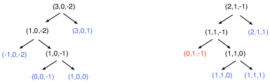
Figure 1: On the left: the algorithm applied to $\chi_{1}=(3,0,-2)$. On the right: the same steps applied to $\chi_{2}=(2,1,-1)$. The vector $(0,1,-1)$ (in red) is not ‘good’.

Now we apply the algorithm one more time and obtain the two vectors $(0,0,-1),(0,1,0)$ whose coordinates are respectively all nonpositive and all nonnegative. Figure 2 shows the final output for the coordinate of $\chi_{1}$ (left hand side) and of $\chi_{2}$ (right hand side).

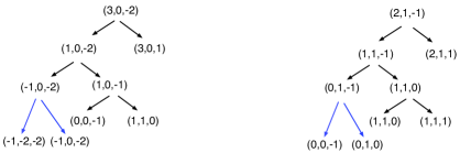
Figure 2: The algorithm of Figure 1 is completed by a further step (blue arrows) since the vector $(0,1,-1)$ was not ‘good’ .

Figure 3 shows that after applying the steps of the algorithm, in the end we subdivide the cone $\{e^{1},e^{2},e^{3}\}$ into the following maximal cones: $\sigma_{1}=\{e^{1},e^{2},e^{1}+e^{3}\}$, $\sigma_{2}=\{e^{1}+2e^{3},e^{2}+e^{3},e^{3}\}$, $\sigma^{3}=\{e^{1}+2e^{3},e^{2},e^{2}+e^{3}\}$, $\sigma^{4}=\{2e^{1}+3e^{3},e^{2},e^{1}+2e^{3}\}$, $\sigma^{5}=\{e^{1}+e^{3},e^{2},2e^{1}+3e^{3}\}$.

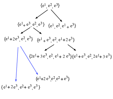
Figure 3: The subdivision of the cone $\{e^{1},e^{2},e^{3}\}$ produced by the steps of the algorithm of Figure 2.

We now give an example of the algorithm applied to a 2-dimensional complete fan. We let $T$ be 2-dimensional and choose a basis of $X^{*}(T)$. The starting fan is then the one whose maximal dimensional cones are the four quadrants with respect to the chosen basis. We then take $\Xi=\{\chi_{1}=(1,0),\chi_{2}=(1,2)\}$. We remark that the algorithm needs to be applied only in the second and fourth quadrants. The reader can easily check that the final output is the fan given in Figure 4.

Figure 4: Fan for $(1,0),(1,2).$

6 The construction of the toric variety $K_{\Delta({\mathcal{A}})}$

As we mentioned in the Introduction, given a toric arrangement ${\mathcal{A}}$ in $T$ the main step in our construction of a projective wonderful model for the complement ${\mathcal{M}}({\mathcal{A}})$ is the construction of a smooth projective toric variety $K_{\Delta({\mathcal{A}})}$ (where $\Delta({\mathcal{A}})$ denotes its fan), containing $T$ as a dense open set.

We will describe $K_{\Delta({\mathcal{A}})}$ by describing its fan $\Delta({\mathcal{A}})$; this in turn will be obtained by a repeated application of the algorithm of Theorem 4.1.

As a first step we choose a basis for the lattice $X^{*}(T)$. This gives an isomorphism of $T$ with $({\mathbb{C}}^{*})^{n}$, an isomorphism of $X^{*}(T)$ with $\mathbb{Z}^{n}$ and of $X_{*}(T)\otimes\mathbb{R}$ with ${\mathbb{R}}^{n}$. The decomposition of ${\mathbb{R}}^{n}$ into quadrants gives a fan $\Delta$ whose associated $T$ variety is isomorphic to $({\mathbb{P}}^{1})^{n}$.

Let us now consider the toric arrangement ${\mathcal{A}}=\{\mathcal{K}_{1},...,\mathcal{K}_{m}\}$, where $\mathcal{K}_{i}=\mathcal{K}_{\Gamma_{i},\phi_{i}}$, and, for every $i=1,...,m$, let $\chi_{i1},...,\chi_{ij_{i}}$ be an integral basis of $\Gamma_{i}\subset X^{*}(T)$. Let $\Xi$ be the set whose elements are the characters $\chi_{is}$, for every $i=1,...,m$ and for every $1\leq s\leq j_{i}$.

By applying Theorem 4.1 to the fan $\Delta$ and to the set $\Xi\subset X^{*}(T)$, we obtain a new fan $\Delta(\mathcal{A})$ such that each character $\chi_{i,s}$ has property $(E)$ with respect to $\Delta(\mathcal{A})$.

Definition 6.1.

A layer $\mathcal{K}_{\Gamma,\phi}$ is a layer for the arrangement ${\mathcal{A}}=\{\mathcal{K}_{1},...,\mathcal{K}_{m}\}$, or a ${\mathcal{A}}$-layer, if it is a connected component of the intersection of some of the $\mathcal{K}_{i}$.

We have thus proved

Proposition 6.1.

Let $\mathcal{A}$ be a toric arrangement. Choose a basis for $X^{*}(T)$ and let $T\subset({\mathbb{P}}^{1})^{n}$ be the corresponding $T$ embedding. There is a fan $\Delta(\mathcal{A})$ such that

1. The $T$ embedding $K_{\Delta({\mathcal{A}})}$ is smooth and it is obtained from $({\mathbb{P}}^{1})^{n}$ by a sequence of blow ups along closures of orbits of codimension 2.

2. Every ${\mathcal{A}}$-layer has property $(E)$ with respect to $\Delta(\mathcal{A}).$

A few observations are in order:

Remark 6.1.

The construction of $\Delta(\mathcal{A})$ strongly depends on

1. The choice of a basis for $X^{*}(T)$.

2. The choice of the set of characters $\Xi$.

3. The strategy in which our algorithms is implemented.

It is desirable to understand whether and how one could develop a more efficient procedure. We observe that, as a geometric counterpart to the combinatorial blowups of fans, we have that the toric variety $K_{\Delta({\mathcal{A}})}$ is obtained from $({\mathbb{P}}^{1})^{n}$ by a sequence of blowups: each blowup is the blowup of a toric T-variety along the closure of a 2-codimensional T-orbit.

Remark 6.2.

Let us consider the linear span $V^{\prime}$ in $V=X^{*}(T)\otimes{\mathbb{R}}$ of the vectors $\chi_{is}$ mentioned above (so $i=1,..,m$ and $1\leq s\leq j_{i}$). If $V^{\prime}\neq X^{*}(T)\otimes{\mathbb{R}}$ we can choose a basis $\eta_{1},...,\eta_{n}$ of $X^{*}(T)$ such that $\eta_{1},...,\eta_{r})$ span $V^{\prime}$ (from the computational point of view it could be useful to pick as many $\eta_{i}$ as possible from the set $\{\chi_{is}\}$). We have an isomorphism $T=({\mathbb{C}}^{*})^{n}$ as $({\mathbb{C}}^{*})^{r}\times({\mathbb{C}}^{*})^{(n-r)}$ and one easily sees that our problem reduces to finding a smooth projective toric variety for the toric arrangement ${\mathcal{A}}$ restricted to $({\mathbb{C}}^{*})^{r}$. So without loss of generality in the sequel we will always suppose $V^{\prime}=V=X^{*}(T)\otimes{\mathbb{R}}$.

7 The arrangement of subvarieties ${\mathcal{L}}$

Given the toric variety $K_{\Delta({\mathcal{A}})}$ constructed in Section 6, we denote by ${\mathcal{Q}}$ the set whose elements are the subvarieties ${\overline{\mathcal{K}}_{i}}$ and the irreducible components $D_{\alpha}$ of the complement $K_{\Delta({\mathcal{A}})}-T$. We then denote by ${\mathcal{L}}$ the poset made by all the connected components of all the intersections of some of the elements of ${\mathcal{Q}}$.

Theorem 7.1.

The family ${\mathcal{L}}$ is an arrangement of subvarieties according to Definition 2.4.

Proof.

Let us consider an element $S\in{\mathcal{L}}$, that is a connected component of the intersection ${\widetilde{S}}$ of some of the elements in $\mathcal{Q}$. If all of these elements are irreducible components $D_{\alpha}$ of the complement $K_{\Delta({\mathcal{A}})}-T$, from the theory of toric varieties we known that $S$ is smooth and that the intersection is clean.

Let us then consider the case when ${\widetilde{S}}$ is the intersection of the closures of some layers of the arrangement ${\mathcal{A}}=\{\mathcal{K}_{1},...,\mathcal{K}_{m}\}$, say $\mathcal{K}_{1}$, $\mathcal{K}_{2}$,…, $\mathcal{K}_{s}$. Therefore $S$ is the closure of a ${\mathcal{A}}$-layer $\mathcal{K}_{\Gamma,\phi}$.

By point 2 of Proposition 6.1, $\mathcal{K}_{\Gamma,\phi}$ has property $(E)$ with respect to $\Delta(\mathcal{A})$ and it then follows from point 1 of Theorem 3.1 that $S$ is a smooth toric variety. By the description of point 1 of Theorem 3.1 it also follows that if we further intersect $S$ with some irreducible components $D_{\alpha}$ of the complement $K_{\Delta({\mathcal{A}})}-T$, we get that the resulting connected components are boundary components of the toric variety $S$, and therefore they are smooth.

It remains to prove that the intersection of two strata $\Lambda_{1},\Lambda_{2}$ in ${\mathcal{L}}$, if it is not empty, satisfies the condition on the tangent space, i.e.,

$$T_{\Lambda_{i}\cap\Lambda_{j},y}=T_{\Lambda_{i},y}\cap T_{\Lambda_{j},y}$$

for every $y\in\Lambda_{i}\cap\Lambda_{j}$.

The inclusion

$$T_{\Lambda_{i}\cap\Lambda_{j},y}\subseteq T_{\Lambda_{i},y}\cap T_{\Lambda_{j},y}$$

is obvious, then it is sufficient to check that the dimensions are the same. We have already proved that $\Lambda_{i}\cap\Lambda_{j}$ is smooth, so $dim\ T_{\Lambda_{i}\cap\Lambda_{j},y}=dim\ \Lambda_{i}\cap\Lambda_{j}$.

Again, let us first consider the case is when $\Lambda_{i}$ and $\Lambda_{j}$ are connected components of the intersection of the closures of some layers of the arrangement ${\mathcal{A}}$. Therefore we can put $\Lambda_{i}=\overline{\mathcal{K}}_{\Gamma_{i},\phi_{i}}$, $\Lambda_{j}=\overline{\mathcal{K}}_{\Gamma_{j},\phi_{j}}$.

Then every connected component of $\Lambda_{i}\cap\Lambda_{j}$ is of the form $\overline{\mathcal{K}}_{\overline{\Gamma},\overline{\phi}}$, where $\overline{\Gamma}$ is the saturation of the lattice $\Gamma_{1}+\Gamma_{2}$.

In the proof of point 1 of Theorem 3.1 we showed, by a local computation in a chart of $K_{\Delta({\mathcal{A}})}$, that the rank of the Jacobian matrix of the equations defining $\overline{\mathcal{K}}_{\overline{\Gamma},\overline{\phi}}$ is equal to the rank of $\overline{\Gamma}$. Therefore the dimension of $\overline{\mathcal{K}}_{\overline{\Gamma},\overline{\phi}}$ is equal to $n-rank\ \overline{\Gamma}$.

Now we observe that the dimension of $T_{\Lambda_{i},y}\cap T_{\Lambda_{j},y}$ is equal to the dimension of the intersection of the kernels of the Jacobian matrices of the equations defining $\overline{\mathcal{K}}_{\Gamma_{i},\phi_{i}}$ and $\overline{\mathcal{K}}_{\Gamma_{j},\phi_{j}}$. This dimension, as one can immediately check, is equal to $n-rank\ (\Gamma_{1}+\Gamma_{2})$. Since $rank\ \overline{\Gamma}=rank\ (\Gamma_{1}+\Gamma_{2})$ this concludes the proof in this case.

Let us now consider the case when $\Lambda_{i}$ (or $\Lambda_{j}$) is equal to $\overline{\mathcal{K}}_{\Gamma_{i},\phi_{i}}$ intersected with some components $D_{\alpha}$ of the complement $K_{\Delta({\mathcal{A}})}-T$. The relevant remark is that in a local chart a component $D_{\alpha}$ has an equation of type $x_{\nu}=0$, therefore if the intersection $\Lambda_{i}\cap\Lambda_{j}$ is not empty the variable $x_{\nu}$ does not appear in the equations that define $\overline{\mathcal{K}}_{\Gamma_{i},\phi_{i}}$ and $\overline{\mathcal{K}}_{\Gamma_{j},\phi_{j}}$.

Up to this, the computation of the dimensions of $T_{\Lambda_{i}\cap\Lambda_{j},y}$ and $T_{\Lambda_{i},y}\cap T_{\Lambda_{j},y}$ is then completely similar to the one of the preceding case.

∎

8 Root systems and related examples

It is important to point out that our proof of Theorem 7.1 shows that, given a toric arrangement $\mathcal{A}=\{\mathcal{K}_{1},\ldots,\mathcal{K}_{m}\}$ and a smooth complete fan $\Theta$, in order for the family ${\mathcal{L}}$ consisting of all connected components of intersections of some of the $\overline{\mathcal{K}}_{i}$ and some components of the complement $K_{\Theta}\setminus T$, to be an arrangement of subvarieties it suffices that each of the $\mathcal{K}_{i}$’s has property $(E)$ with respect to $\Theta$.

This fact allows us to give a class of examples for which we do not have to go through the complicated algorithm of Section 4.

We first notice that Theorem 3.1 provides another point of view on our construction of the toric variety in the case of a divisorial arrangement. Let us consider the divisorial toric arrangement ${\mathcal{A}}=\{\mathcal{K}_{\chi_{1},b_{1}},...,\mathcal{K}_{\chi_{m},b_{m}}\}$ in $T$, where $\Gamma_{i}={\mathbb{Z}}\chi_{i}$, $\chi_{i}$ a primitive character. In $V=hom_{\mathbb{Z}}(X^{*}(T),{\mathbb{R}})$ take the real hyperplane arrangement $\mathcal{H}_{\mathcal{A}}=\{H_{\chi_{1}},...,H_{\chi_{m}}\}$ of the hyperplanes orthogonal to the $\chi_{i}$’s. The chambers of this hyperplane arrangement define some $n$-dimensional rational polyhedral cones, which we can assume to be strongly convex (see Remark 6.2). Taking all non empty intersections of (the closures of ) these chambers, we obtain a complete fan $\Phi$, that is not necessarily smooth: as a consequence of Theorem 3.1 (see Remark 3.2) we have that the fan $\Delta({\mathcal{A}})$ provided by our algorithm gives a particular subdivision of this fan but any smooth complete fan subdividing $\Phi$ would do.

If it happens that $\Phi$ is already a smooth projective fan then there is no need to apply our algorithm so that the toric variety $K_{\Phi}$ gives a canonical choice for our construction.

Here is the main example of this situation. Suppose $T$ is the maximal torus in an adjoint semisimple group $G$ and $R\subset X^{*}(T)$ is the corresponding root system. We choose a set of positive roots $R^{+}$ and fix for each $\alpha\in R^{+}$ a constant $b_{\alpha}\in{\mathbb{C}}^{*}$ We then get the toric arrangement $\mathcal{A}=\{\mathcal{K}_{\alpha,b_{\alpha}}\}_{\alpha\in R^{+}}$. It is immediate from the definition that the corresponding fan $\Phi$ in $V=hom_{\mathbb{Z}}(X^{*}(T),{\mathbb{R}})$ is given by the Weyl chambers and their faces. Also each Weyl chamber corresponds to a choice of a basis of simple roots and every root is expressed as a linear combination with respect to such a basis with all non negative or non positive coefficients.

If we then take the family ${\mathcal{L}}$ of the connected components of all the intersections of the closures of $\overline{\mathcal{K}}_{\alpha,b_{\alpha}}$ and of boundary divisors in $K_{\Phi}$ we get

Proposition 8.1.

The family ${\mathcal{L}}$ is an arrangement of subvarieties in $K_{\Phi}$.

Remark 8.1.

1) The variety $K_{\Phi}$ appears in various relevant instances, for example as the closure of a “generic" $T$ orbit in the flag variety, or as the closure of $T$ in the wonderful compactification of $G$.

2) If $W$ denotes the Weyl group of the root system $R$, $W$ acts on the embedding $K_{\Phi}$ compatibly with its action on $T$. Now, if for a negative root $\alpha$, we set $b_{\alpha}=b_{-\alpha}^{-1}$, we obtain a map $R\to{\mathbb{C}}^{*}$. If this map is constant on $W$-orbits then $W$ also acts on $\mathcal{A}$ and on the family ${\mathcal{L}}$. So taking a building set stable under the $W$ action we obtain a $W$ equivariant compactification of $\mathcal{A}$.

Notice that obviously the embedding $K_{\Phi}$ works as well for any arrangement $\mathcal{A}^{\prime}\subset\mathcal{A}$.

For instance, given a directed graph $\Gamma$, one can associate to its vertices $\gamma_{1},...,\gamma_{n+1}$ the vectors $e_{1},...,e_{n+1}$ of a basis of ${\mathbb{Z}}^{n}$, and to its arrows their incidence vectors (if an arrow connects $\gamma_{i}$ and $\gamma_{j}$ and points to $\gamma_{j}$ we associate to it the vector $e_{i}-e_{j}$). If we think the root system of type $A_{n}$ as the set of vectors $\alpha_{i,j}=e_{i}-e_{j}$, where $i,j=1,\ldots n+1$ and $i\neq j$, then to such a directed graph it is associated the subset of $\mathcal{A}$ (for $A_{n}$) consisting of those $\mathcal{K}_{\alpha,b_{\alpha}}$ for which $\alpha=e_{i}-e_{j}$ comes from an arrow of our graph.

9 A simple remark on the integer cohomology and on the Chow ring of a projective model

Let us consider a toric arrangement ${\mathcal{A}}$ and denote by $\mathcal{W}({\mathcal{A}})$ any projective wonderful model for ${\mathcal{A}}$ constructed according to the strategy described in this paper. We will prove that the integer cohomology of $\mathcal{W}({\mathcal{A}})$ is even and torsion free and that the integer cohomology ring is isomorphic to the Chow ring.

Let us start by recalling from [8] the definition of property $(S)$ for a smooth projective algebraic variety. If X is an smooth and projective algebraic variety, let us denote by $A^{k}(X)$ the group generated by the $k$-codimensional irreducible subvarieties modulo rational equivalence (see [21] 1.3) and by $A^{*}(X)$ the Chow ring.

Let $H^{j}(X)$ be the integer cohomology of X. There is a canonical ring homomorphism (see for instance [21] 19.1 or [4] 12.5):

$$\Phi:A^{*}(X)\to H^{*}(X)$$

that sends $A^{j}(X)\to H^{2j}(X)$ for every $j$.

The following definition is adapted from [8] (we are specializing to our case where Poincaré duality holds).

Definition 9.1.

A smooth and projective algebraic variety X is said to have property $(S)$ if

1. $H^{i}(X)=0$ for $i$ odd and $H^{j}(X)$ has no torsion for even $j$.

2. $\Phi_{|A^{j}}:A^{j}(X)\mapsto H^{2j}(X)$ is an isomorphism for all $j\geq 0.$

In particular, if a smooth projective algebraic variety X satisfies property $(S)$ we have that $\Phi$ gives a ring isomorphism $A^{*}(X)\cong H^{*}(X)$.

Theorem 9.1.

The projective wonderful variety $\mathcal{W}({\mathcal{A}})$ has property $(S)$.

Proof.

We start by remarking that if we have two smooth complete subvarieties $Y\subset X$ such that both $Y$ and $X$ have property $(S)$, then also the blowup $\widetilde{X}={Bl}_{Y}X$ of $X$ along $Y$ has property $(S)$. Indeed recall (see for instance Theorem 15.11 in [17]) that, setting $E$ equal to the exceptional divisor, we have the exact sequence of Chow groups

$$0\rightarrow A(Y)\rightarrow A(X)\oplus A(E)\rightarrow A(\widetilde{X})\rightarrow 0$$

Since $E$ is a projective bundle over $Y$, then $E$ has property $(S)$. Also, since $Y$, $X$ and $E$ have no odd cohomology, we get, by comparing the exact sequence above with the corresponding sequence for cohomology, that also $\widetilde{X}$ has the property $(S)$.

This allows us to prove inductively that the projective model $\mathcal{W}({\mathcal{A}})$ has the property $(S)$. We start by observing that $\mathcal{W}({\mathcal{A}})$ is constructed by the blowup process described by MacPherson-Procesi and Li (see Theorem 2.1) starting from the smooth projective toric variety $K_{\Delta({\mathcal{A}})}$. Now from the theory of toric varieties we know that a smooth projective toric variety has the property $(S)$ (see for instance [4] 12.5).

As we noticed in Remark 3.2, from Theorem 3.1 and from the standard theory of toric varieties we know that also all the strata in $\mathcal{L}$ are smooth projective toric varieties.

So in the first step of the construction we blow up a smooth projective toric variety along a stratum that is isomorphic to a smooth projective toric variety. The resulting variety has property $(S)$ and also the proper transforms of the other strata have property $(S)$, since (again by Theorem 3.1 and standard theory of toric varieties) they are blowups of smooth projective toric varieties along smooth projective toric subvarieties.

By induction on the dimension one can immediately see that at every step of the blowup process we blow up a variety that has property $(S)$ along a subvariety that has property $(S)$. ∎

References

• [1] Callegaro, F., and Delucchi, E. The integer cohomology algebra of toric arrangements. arXiv:1504.06169 (2015).
• [2] Callegaro, F., and Gaiffi, G. On models of the braid arrangement and their hidden symmetries. Int Mat Res Notices, 21 (2015), 11117 – 11149.
• [3] Callegaro, F., Gaiffi, G., and Lochak, P. Divisorial inertia and central elements in braid groups. Journal of Algebra 457 (2016), 26 – 44.
• [4] Cox, D.Β A., Little, J.Β B., and Schenck, H.Β K. Toric varieties, vol.Β 124 of Graduate Studies in Mathematics. American Mathematical Society, Providence, RI, 2011.
• [5] D’Adderio, M., and Moci, L. Arithmetic matroids, the Tutte polynomial and toric arrangements. Adv. Math. 232 (2013), 335–367.
• [6] d’Antonio, G., and Delucchi, E. A Salvetti complex for toric arrangements and its fundamental group. Int. Math. Res. Not., 15 (2012), 3535–3566.
• [7] d’Antonio, G., and Delucchi, E. Minimality of toric arrangements. J. Eur. Math. Soc. (JEMS) 17, 3 (2015), 483–521.
• [8] DeΒ Concini, C., Lusztig, G., and Procesi, C. Homology of the zero-set of a nilpotent vector field on a flag manifold. J. Amer. Math. Soc. 1, 1 (1988), 15–34.
• [9] DeΒ Concini, C., and Procesi, C. Complete symmetric varieties. II. Intersection theory. In Algebraic groups and related topics (Kyoto/Nagoya, 1983), vol.Β 6 of Adv. Stud. Pure Math. North-Holland, Amsterdam, 1985, pp.Β 481–513.
• [10] DeΒ Concini, C., and Procesi, C. Hyperplane arrangements and holonomy equations. Selecta Mathematica 1 (1995), 495–535.
• [11] DeΒ Concini, C., and Procesi, C. Wonderful models of subspace arrangements. Selecta Mathematica 1 (1995), 459–494.
• [12] DeΒ Concini, C., and Procesi, C. On the geometry of toric arrangements. Transform. Groups 10 (2005), 387–422.
• [13] DeΒ Concini, C., and Procesi, C. Topics in Hyperplane Arrangements, Polytopes and Box-Splines. Springer, Universitext, 2010.
• [14] DeΒ Concini, C., Procesi, C., and Vergne, M. Vector partition functions and index of transversally elliptic operators. Transform. Groups 15, 4 (2010), 775–811.
• [15] Denham, G. Toric and tropical compactifications of hyperplane complements. Ann. Fac. Sci. Toulouse Math. (6) 23, 2 (2014), 297–333.
• [16] Drinfeld, V. On quasi triangular quasi-hopf algebras and a group closely connected with $Gal(\overline{{\mathbb{Q}}}/{\mathbb{Q}})$. Leningrad Math. J. 2 (1991), 829–860.
• [17] Eisenbud, D., and Harris, J. 3264 and All That, A second course in algebraic geometry. Cambridge University Press, Cambridge, 2016.
• [18] Etingof, P., Henriques, A., Kamnitzer, J., and Rains, E. The cohomology ring of the real locus of the moduli space of stable curves of genus 0 with marked points. Annals of Math. 171 (2010), 731–777.
• [19] Feichtner, E. De Concini-Procesi arrangement models - a discrete geometer’s point of view. Combinatorial and Computational Geometry, J.E. Goodman, J. Pach, E. Welzl, eds; MSRI Publications 52, Cambridge University Press (2005), 333–360.
• [20] Feichtner, E., and Sturmfels, B. Matroid polytopes, nested sets and Bergman fans. Port. Math. (N.S.) 62 (2005), 437–468.
• [21] Fulton, W. Intersection theory, secondΒ ed., vol.Β 2 of Ergebnisse der Mathematik und ihrer Grenzgebiete. 3. Folge. A Series of Modern Surveys in Mathematics [Results in Mathematics and Related Areas. 3rd Series. A Series of Modern Surveys in Mathematics]. Springer-Verlag, Berlin, 1998.
• [22] Fulton, W., and MacPherson, R. A compactification of configuration spaces. Annals of Mathematics 139, 1 (1994), 183–225.
• [23] Gaiffi, G. Permutonestohedra. Journal of Algebraic Combinatorics 41 (2015), 125–155.
• [24] Gaiffi, G., and Serventi, M. Families of building sets and regular wonderful models. European Journal of Combinatorics 36 (2014), 17–38.
• [25] Henderson, A. Representations of wreath products on cohomology of De Concini-Procesi compactifications. Int. Math. Res. Not., 20 (2004), 983–1021.
• [26] Hu, Y. A compactification of open varieties. Trans. Amer. Math. Soc (2003), 4737–4753.
• [27] Li, L. Wonderful compactification of an arrangement of subvarieties. Michigan Math. J. 58 (2009), 535–563.
• [28] Looijenga, E. Cohomology of ${\mathcal{M}}_{3}$ and ${\mathcal{M}}^{1}_{3}$. In Mapping class groups and moduli spaces of Riemann surfaces (GΓΆttingen, 1991/Seattle, WA, 1991), vol.Β 150 of Contemp. Math. Amer. Math. Soc., Providence, RI, 1993, pp.Β 205–228.
• [29] MacPherson, R., and Procesi, C. Making conical compactifications wonderful. Selecta Mathematica 4, 1 (1998), 125–139.
• [30] Moci, L. Combinatorics and topology of toric arrangements defined by root systems. Atti Accad. Naz. Lincei Cl. Sci. Fis. Mat. Natur. Rend. Lincei (9) Mat. Appl. 19, 4 (2008), 293–308.
• [31] Moci, L. A Tutte polynomial for toric arrangements. Trans. Amer. Math. Soc. 364, 2 (2012), 1067–1088.
• [32] Moci, L. Wonderful models for toric arrangements. Int. Math. Res. Not., 1 (2012), 213–238.
• [33] Rains, E. The homology of real subspace arrangements. J Topology 3 (4) (2010), 786–818.
• [34] Ulyanov, A. Polydiagonal compactifications of configuration spaces. J. Algebraic Geom (2002), 129–159.
• [35] Yuzvinsky, S. Cohomology bases for De Concini-Procesi models of hyperplane arrangements and sums over trees. Invent. math. 127 (1997), 319–335.