LiRa: A New Likelihood-Based Similarity Score For Collaborative Filtering

Abstract

Recommender system data presents unique challenges to the data mining, machine learning, and algorithms communities. The high missing data rate, in combination with the large scale and high dimensionality typical of recommender systems data, requires new tools and methods for efficient data analysis. Here, we address the challenge of evaluating similarity between users in a recommender system, where for each user only a small set of ratings is available. We present a new similarity score, that we call LiRa, based on a statistical model of user similarity for large-scale, discrete valued data with many missing values. We show that this likelihood ratio-based score is more effective at identifying similar users than traditional similarity scores in user-based collaborative filtering, such as the Pearson correlation coefficient. We argue that our approach has significant potential to improve both accuracy and scalability in collaborative filtering.

<ccs2012> <concept> <concept_id>10002951.10003227.10003351.10003269</concept_id> <concept_desc>Information systems Collaborative filtering</concept_desc> <concept_significance>500</concept_significance> </concept> <concept> <concept_id>10002951.10003317.10003338.10003342</concept_id> <concept_desc>Information systems Similarity measures</concept_desc> <concept_significance>500</concept_significance> </concept> <concept> <concept_id>10002951.10003317.10003338.10010403</concept_id> <concept_desc>Information systems Novelty in information retrieval</concept_desc> <concept_significance>300</concept_significance> </concept> <concept> <concept_id>10002951.10003227.10003351.10003445</concept_id> <concept_desc>Information systems Nearest-neighbor search</concept_desc> <concept_significance>100</concept_significance> </concept> </ccs2012>

[500]Information systems Collaborative filtering [500]Information systems Similarity measures [300]Information systems Novelty in information retrieval [100]Information systems Nearest-neighbor search

1 Introduction

Recommender systems arose as a way to provide personalized recommendations, in a setting where the number of available items, products, or options to a user is too large to sift through manually. Collaborative filtering has proven to be an effective approach for recommendation, relying on the similarity of users or items in a system to predict future user preferences. The premise underlying user-based collaborative filtering is that similar users tend to rate items similarly, therefore to predict how a user $u$ will rate an item $i$, we should look at the ratings given to $i$ by users similar to $u$. In item-based collaborative filtering, the assumption is that similar items tend to be rated similarly by the users, therefore the rating prediction should be based on the ratings given by user $u$ to items similar to $i$. A central component of any collaborative filtering algorithm is the choice of similarity score that is used to evaluate user-user or item-item similarity.

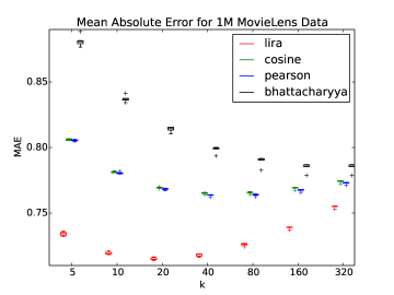
Figure 1: Prediction accuracy of the kNN method using several similarity scores on the 1M MovieLens dataset. The LiRa similarity attains the lowest MAE across tested values of $k$. The greater difference between LiRa and other scores at lower values of $k$ indicate its better ability to find similar users.

Despite many improvements and successes of modern model-based collaborative filtering, the k-Nearest-Neighbor (kNN) method remains a popular and widely used approach, in large part due to its simplicity and scalability.[8] To perform user-based collaborative filtering, the kNN method predicts the rating $p_{ui}$ for an item $i$ by a user $u$ by selecting the $k$ most similar users to user $u$ who have rated item $i$. The prediction $p_{ui}$ is then computed by averaging the ratings given to item $i$ by these $k$ similar users. Similarly, in item-based kNN, the ratings of the $k$ items most similar to item $i$ and rated by user $u$ are used to compute $p_{ui}$. Many variants of kNN have been proposed and investigated in order to provide guidelines for optimal parameter settings and implementation choices. The choice of similarity score has consistently been shown to be highly influential on rating prediction accuracy. [8, 11, 16, 1]

In this work, we present a new similarity score, called LiRa, for large-scale, discrete-valued and high-dimensional data with many missing values. We use an empirical evaluation on real data to show its effectiveness in finding similar users in user-based collaborative filtering.We also present an evaluation of several similarity scores’ ability to detect clustered points in synthetic data sets, revealing fundamental properties of these scores that are important in their application to recommender system data.

2 Motivation and Background

Our work stems from a well-known problem in collaborative filtering: RS data is often very sparse, meaning that in a system with $m$ users and $n$ items, the number of ratings observed is typically much less than the $mn$ user-item pairs. Thus in approaches that seek to predict future ratings based on user-user or item-item similarity, it is important to consider how the sparsity of ratings affects the similarity score.

Popular choices of similarity scores for user-based collaborative filtering include the Pearson correlation coefficient and the cosine similarity, which are “commonly accepted as the best choice."[17] We review these traditional scores briefly to highlight the core issue that will be addressed with our new similarity score, presented in Section 3.

For two users $u$ and $v$, let $I_{uv}$ be the set of co-rated items, i.e. those items that were rated by both $u$ and $v$. Let $r_{ui}$ be the rating given to item $i$ by user $u$. Then, the Pearson correlation between users $u$ and $v$, $PC(u,v)$, is defined as follows [17]:

$$PC(u,v)=\frac{\sum_{i\in I_{uv}}(r_{ui}-\bar{r}_{u})(r_{vi}-\bar{r}_{v})}{\sqrt{\sum_{i\in I_{uv}}(r_{ui}-\bar{r}_{u})^{2}\sum_{i\in I_{uv}}(r_{vi}-\bar{r}_{v})^{2}}}$$ (1)

where $\bar{r}_{u}$ is the average rating given by user $u$ to the items in $I_{uv}$, and similarly for $\bar{r}_{v}$. The Pearson correlation is a measure of linear correlation between user $u$ and $v$’s ratings, and takes on values between -1 and 1.

The Cosine Vector similarity between users $u$ and $v$, or $CV(u,v)$, is a measure of the angle between the $N$-dimensional vectors defined by user $u$ and $v$’s ratings. More specifically, if we let $y_{u}\in R^{N}$ be the vector with $y_{ui}=r_{ui}$ for rated item $i$, and $y_{ui}=0$ otherwise, then:

$$CV(u,v)=\frac{y_{u}^{T}y_{v}}{||y_{u}||||y_{v}||}=\frac{\sum_{i\in I_{uv}}r_{ui}r_{vi}}{\sqrt{\sum_{i\in I_{u}}r_{ui}^{2}\sum_{j\in I_{v}}r_{vj}^{2}}}$$ (2)

where $I_{u}$, $I_{v}$ are the sets of items rated by $u$ and $v$, respectively. The cosine of the angle between two vectors ranges from -1 to 1, with 1 indicating perfectly matching entries in both vectors. A CV similarity of 1, therefore, indicates perfectly matching entries. However, although a cosine of 0 indicates orthogonal vectors in an $N$-dimensional vector space, the cosine of two rating vectors will only be 0 if the there are no co-rated items in raw (unnormalized) data.

A major issue with both of these scores is their lack of consideration for missing data. Although the PC similarity, which is equivalently the sample Pearson correlation coefficient, is a consistent estimator of the population correlation coefficient for large sample sizes, the number of co-rated items between $u$ and $v$, or $|I_{uv}|$, is often so small that the PC similarity is not reliable.

Similarly, we can think of the Cosine Vector similarity as the cosine of the angle between two vectors that represent the projection of user ratings onto the space spanned by the $|I_{u}\cup I_{v}|$ dimensions in which data is observed, but the value of this angle in higher dimensions has is treated the same as its value in lower dimensions.

We conclude this explanation of the drawbacks of popular similarity scores used on RS data with the following example. Suppose we want to compute the similarity between two users represented by the following identical rating vectors, constructed by following the definition of vectors used by the CV similarity:

$$y_{u}=\left[\begin{array}[]{cccccc}1&1&0&0&0&2\end{array}\right],\\ y_{v}=\left[\begin{array}[]{cccccc}1&1&0&0&0&2\end{array}\right]$$ (3)

Both CV and Pearson will yield a score of 1 between $u$ and $v$. If we increase the amount of data observed, leaving the vectors identical:

$$x_{u}=\left[\begin{array}[]{cccccc}1&1&5&4&4&2\end{array}\right]x_{v}=\left[\begin{array}[]{cccccc}1&1&5&4&4&2\end{array}\right]$$ (4)

the CV and Pearson similarities will remain the same.

However, we have observed twice as much data in the second case – shouldn’t our similarity score reflect more confidence in the similarity computation as we increase the amount of data we have available for input? This question motivated us to derive a new similarity score, which we refer to as the Likelihood Ratio, or LiRa, similarity.

3 The Likelihood Ratio Similarity

The idea to use a likelihood-based score for similarity computations in RS data was inspired in part by the LOD score popular in genetic mapping [5] and the concept of modularity in community detection [14]. In both cases, the concept of similarity is based on comparing the likelihood of the observed data, under some assumptions on the underlying data structure, to the likelihood of observing the data by chance. In genetic mapping, the LOD score relates the likelihood of observing genetic marker data, assuming genetic linkage, to the likelihood of observing the same genotypes by chance. Newman [14] introduced the idea that a community structure contains many more edges than expected if the edges among social network vertices were generated at random. Extending these ideas to the RS domain, we present the Likelihood Ratio Similarity.

3.1 Definition of the LiRa Similarity

For two discrete-valued vectors $x_{u}$ and $x_{v}$, we define the Likelihood Ratio (LiRa) Similarity as follows:

$$\textnormal{LiRa}(x_{u},x_{v})=\log_{10}\frac{p(\textnormal{differences in }x_{u}\textnormal{ and }x_{v}\textnormal{| same cluster })}{p(\textnormal{differences in }x_{u}\textnormal{ and }x_{v}|\textnormal{ pure chance})}$$ (5)

where the numerator in the ratio is the probability of observing the values in $x_{u}$ and $x_{v}$, assuming $x_{u}$ and $x_{v}$ belong to the same cluster in our cluster model, and the probability in the denominator is set by assuming that the entries in $x_{u}$ and $x_{v}$ were generated uniformly at random.

Suppose that the entries in each vector can take on only a finite number $d$ of discrete values $\mathcal{V}=\{1,2,\dots,d\}$. Then, we can easily compute the probability that we observe the values $x_{ui}$ and $x_{vi}$ for co-observed entry $i$ by chance, assuming that the values are generated uniformly and independently at random. This is probability is simply $\frac{1}{d^{2}}$. Therefore, the probability that the two vectors match exactly in a particular entry $i$ is $p(|x_{ui}-x_{vi}|=0)=\frac{d}{d^{2}}=\frac{1}{d}$. Similarly, we can easily derive $p(|x_{ui}-x_{vi}|=\delta)$ for $\delta=1,...,d-1$. The denominator in the ratio in LiRa is thus defined as:

$$p(\textnormal{differences in }x_{u}\textnormal{ and }x_{v}|\textnormal{ pure chance})=\prod_{\delta=0}^{d-1}b_{\delta}^{\#\delta}$$ (6)

where $b_{\delta}=p(|x_{ui}-x_{vi}|=\delta)$, assuming that $x_{ui}$ and $x_{vi}$ were generated by a uniform distribution over the values $\mathcal{V}$, and $\#\delta$ is the number of times that we observe a difference of $\delta$ in the co-observed entries.

The challenge is to define the probability of observing a difference of $\delta$ in the values $x_{ui}$ and $x_{vi}$, under the assumption that $x_{u}$ and $x_{v}$ belong to the same cluster. This is not a trivial task, and we argue that this model will be dependent on the application of interest. For RS data, we make two assumptions that we believe lead to one plausible model: (1) An underlying cluster structure exists in RS data: There exist a set of clusters $\mathcal{C}_{1},...,\mathcal{C}_{\kappa}$ such that each user $u$ belongs to at least one $\mathcal{C}_{c}$, and (2) The probability distribution on differences in user ratings is fixed within a cluster, with a greater probability of observing matching than mismatched ratings. These assumptions encapsulate the intuition that similar users tend to rate items similarly.

With these assumptions, we define the following probability distribution over the differences $|x_{ui}-x_{vi}|$:

$$c_{\delta}=p(|x_{ui}-x_{vi}|=\delta|\textnormal{ same cluster})=\left(\frac{1}{2}\right)^{\delta+1}$$ (7)

with the exception that

$$c_{d-1}=p(|x_{ui}-x_{vi}|=d-1)=1-\sum_{\delta=0}^{d-2}c_{\delta}=\frac{1}{2^{d-1}}$$ (8)

to ensure a proper probability distribution. Therefore the numerator in the ratio in LiRa becomes:

$$p(\textnormal{differences in }x_{u}\textnormal{ and }x_{v}|\textnormal{ same cluster })=\prod_{\delta=0}^{d-1}c_{\delta}^{\#\delta}$$ (9)

where $c_{\delta}$ and $\#\delta$ are defined above, and $x_{ui}=r_{ui}$ if user $u$ rated item $i$, and $-$ otherwise, where $-$ indicates a missing value.

We emphasize that both $x_{u}$ and $x_{v}$ may have many missing values, which are not taken into account when evaluating these probabilities. In particular, the values are not simply treated as 0’s as in the Cosine Vector similarity score. On the other hand, as long as $\frac{1}{2}>\frac{1}{d}$, the LiRa score increases with a greater number of matching co-observed entries, and in general the contribution to the LiRa score of the rating difference for a co-observed item $i$ will depend on the number of discrete values $d$. For example, with $d=5$, $b_{1}>c_{1}$, but at $d=10$, $b_{1}<c_{1}$, thus a difference of 1 in a rating scale of 1 to 5 will decrease the LiRa score, whereas on a rating scale of 1 to 10, a difference of 1 in user ratings will increase it. To see this, notice we can re-write the LiRa score as:

$$\sum_{d=1}^{\delta}(\#\delta)\log_{10}\left(\frac{c_{\delta}}{b_{\delta}}\right)$$ (10)

and thus $\log_{10}\left(c_{\delta}/b_{\delta}\right)$ is the amount that a pair of co-observed ratings $x_{ui}$ and $x_{vi}$ with a rating difference of $\delta$ will contribute to the similarity score.

In future work, we plan to explore other, perhaps more plausible, multinomial probability distributions over the differences in user ratings that capture the intuition that users in the same cluster should rate items with very close rating values. However, we claim that this simple model captures enough of the intuition that users with similar preferences are more likely to agree than disagree in their ratings of the same item. We will show in Section 4 that these assumptions lead to a useful similarity score for RS data.

We conclude with an example using the same the vectors $y_{u}$ and $y_{v}$ from Equation 3. The corresponding vectors $x_{u}$ and $x_{v}$ are:

$$x_{u}=\left[\begin{array}[]{cccccc}1&1&-&-&-&2\end{array}\right],\\ x_{v}=\left[\begin{array}[]{cccccc}1&1&-&-&-&2\end{array}\right]$$

Suppose that there are $d=5$ discrete rating values in the data set. We get the LiRa similarity:

$$\textnormal{LiRa}(x_{u},x_{v})=\log_{10}\frac{(\frac{1}{2})^{3}}{(\frac{1}{5})^{3}}=1.19$$ (11)

Now consider LiRa$(x_{u},x_{v})$ when we observe the full vectors:

$$x_{u}=\left[\begin{array}[]{cccccc}1&1&5&4&4&2\end{array}\right],\\ x_{v}=\left[\begin{array}[]{cccccc}1&1&5&4&4&2\end{array}\right]$$

Now, we have:

$$\textnormal{LiRa}(x_{u},x_{v})=\log_{10}\frac{(\frac{1}{2})^{6}}{(\frac{1}{5})^{6}}=2.39$$ (12)

With twice as much data, the LiRa similarity is twice as high. Note that, in particular, the maximum LiRa score for any two vectors is always attained when the two vectors are equal, but that the similarity grows as $O(n\log_{10}d)$, where $n$ is the dimensionality of the input vectors and $d$ is again the number of discrete rating values. Contrast this with the Pearson or Cosine similarities, which will attain a maximum of 1, regardless of the amount of data observed.

Like modularity in community detection and the LOD score in genetic mapping, the LiRA similarity makes assumptions on the underlying data structure in order to better evaluate similarity among entities in the data.

4 Empirical Evaluation

We evaluate the effectiveness of the LiRa similarity in comparison to other similarity scores in RS data in two ways: (1) We compare the prediction accuracy of a simple kNN method using various similarity scores on real data sets, and (2) We evaluate the ability of several similarity scores to distinguish points within the same cluster from points in different clusters in synthetic data. Experiments on real data sets show that the LiRa similarity can detect similar users in a realistic setting with better accuracy than other scores. The synthetic data allows us to observe the effect of missing entries and dimensionality on similarity computations, and to verify that the LiRa score detects users from the same cluster when a known clustering exists within the data.

4.1 Data

As Herlocker et al. note in their overview of methods for evaluating recommender systems [12], there are few publicly available data sets that can be used to test hypotheses about RS data, forcing most research in this field to experiment on the few available data sources. Our source of real data are the publicly available MovieLens data sets, which are among the most often referenced data sets in RS literature [3]. Here, we report results on the 100K and 1M MovieLens data sets. For the 100K dataset, we used the u1-u5 .base and .test sets when evaluating prediction accuracy. For the 1M dataset, we randomly split the original rating data into five sets of 80%/20% training/test pairs.

In addition to our empirical evaluation on real data, we generated a small set of synthetic data sets. The publicly available data sets we are aware of are not rich enough to examine the effects we are intersted in evaluating – most already contain very high missing rates, thus simply deleting existing entries to simulate more missing data would result in a very limited range of test cases for experimentation. Our experiments on synthetic data give us an in-depth view of the effects of missing entries in RS data.

4.2 Experiments on Real Data

We first give the pertinent details of our implementation of the kNN algorithm, which is used to evaluate the effectivenes of a similarity score in detecting users with similar preferences. For each rating $r_{ui}$ that user $u$ gave to item $i$ in the test set, we first find at most $k$ nearest neighbors of user $u$ in the training set, among those who rated item $i$. Each neighbor $v$ of $u$ has the property that the similarity $S(u,v)$ is greater than or equal to $S(u,z)$ for any other user $z$ in the training set, where $S(u,v)$ is the similarity score between $u$ and $v$ in the training set. The number of neighbors is less than $k$ if less than $k$ users rated item $i$ in the training set. Next, the prediction $p_{ui}$ of the rating that user $u$ gives item $i$ is computed by taking an unweighted average of the ratings that the neighbors of $u$ have item $i$.

The Root Mean Squared Error (RMSE) “is perhaps the most popular metric used in evaluating accuracy of predicted ratings”  [10]. Another popular measure of prediction accuracy is the Mean Absolute Error (MAE). The RMSE and MAE are defined as follows:

$$RMSE=\sqrt{\sum_{r_{ui}\in\mathcal{T}}(r_{ui}-p_{ui})^{2}}\textnormal{ , }MAE=\sum_{r_{ui}\in\mathcal{T}}|r_{ui}-p_{ui}|$$

where $\mathcal{T}$ is the test set of ground truth ratings. We report both the RMSE and MAE for ratings predicted by the kNN method for various values of $k$ and several similarity scores.

In addition to the Pearson, Cosine and LiRa scores, we evaluate the kNN prediction accuracy using Patra et al.’s recently proposed BCF score [16]. The Bhattacharyya coefficient for collaborative filtering (BCF) attempts to use global item similarities as weights in local user rating similarity computations, and was reported to perform well on extremely sparse data sets. It is defined as follows:

$$\textstyle\textnormal{BCF}(x_{i},x_{j})=\textnormal{Jacc}(x_{i},x_{j})+\sum_{i\in I_{u}}\sum_{j\in I_{v}}BC(i,j)\textnormal{loc}(x_{ui},x_{vj})$$ (13)

where

$$BC(i,j)=\sum_{\rho=1}^{d}\sqrt{\frac{\#\rho_{i}}{\#i}\frac{\#\rho_{j}}{\#j}}$$

where $d$ is the number of rating values, $\#i$ is the number of users that rated item $i$, and $\#\rho_{i}$ is the number of users that rated item $i$ with value $\rho$. $I_{u}$, $I_{v}$, and $I_{uv}$ are defined as in Section 2. Thus $BC$ gives more weight to the local similarity $\textnormal{loc}(x_{ui},x_{vj})$ if items $i$ and $j$ have similar rating distributions across users in the entire training set. $\textnormal{loc}(x_{ui},x_{vj})$ is a local similarity measure of the ratings that user $u$ gave to item $i$ and user $v$ gave to item $j$. Of the two loc similarity scores defined by Patra et al., we chose to use $\textnormal{loc}_{\textnormal{corr}}$, defined as:

$$\textnormal{loc}_{\textnormal{corr}}(x_{u},x_{v})=\frac{\left(x_{ui}-\bar{x}_{u}\right)\left(x_{vj}-\bar{x}_{v}\right)}{\sigma_{u}\sigma_{v}}$$

where $\sigma_{u}$ is the standard deviation of ratings made by user $u$ and $\bar{x}_{u}$ is the mean of ratings made by user $u$. In the experimental evaluation of Patra et al., $\textnormal{loc}_{\textnormal{corr}}$ achieved lower rating prediction error than their other loc similarity score. Jacc$(x_{u},x_{v})$ is the Jaccard similarity:

$$\textnormal{Jacc}(x_{u},x_{v})=\frac{|I_{uv}|}{|I_{u}|+|I_{v}|}$$

4.3 kNN Results

The MAE and RMSE for kNN prediction on the MovieLens 100K data sets are shown in Figure 2, with the MovieLens 1M MAE results in Figure 1. Note that the LiRa similarity outperforms other similarity scores in prediction accuracy and for a wide range of choices for the number of neighbors $k$.

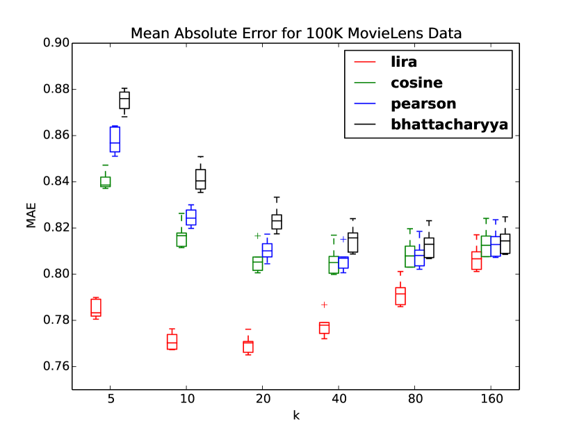
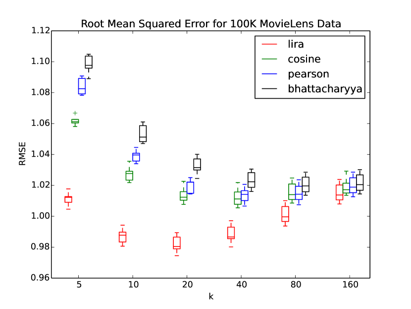
Figure 2: Comparison of prediction accuracy using various similarity scores in kNN show LiRa’s better ability to choose relevant neighbors.

We include both the MAE and RMSE results for the 100K data sets, but omit the RMSE for the 1M data sets due to space constraints. However, the RMSE results for the 1M data sets show the same trend as is seen in the MAE results – that is, LiRa dominates the other similarity scores in accuracy, and the gap between LiRa and other similarity scores’ prediction error widens both when we increase the size of the data set, and when we decrease $k$.

The kNN curves have the expected shape – at low values of $k$, the data is being under-utilized, because there are on average more than $k$ users who rated item $i$ and are truly similar to $u$ in the data, but they are being left out of the computation of the prediction $p_{ui}$. At the other extreme, at very high values of $k$, there are on average less than $k$ truly similar users to $u$ in the data who rated item $i$, and the additional users in the neighbor set are not useful in predicting $u$’s rating of item $i$.

However, the best value of $k$ for LiRa tends to be lower than the best value of $k$ using other similarity scores, and the LiRa score outperforms other similarity scores for all values of $k$ where the neighbor set is not so large that it is virtually the same for each similarity score (at $k=160$, the number of neighbors is 17% of the 100K training set size, meaning that for most users, the prediction $p_{ui}$ is based on all users in the training set who rated item $i$). In addition, as $k$ decreases, the gap between LiRa and the other scores’ error widens. From these observations, we conclude that LiRa is better able to distinguish between truly similar and truly dissimilar users; for a given $k$, it finds a better set of $k$ neighbors than the other scores, and as $k$ decreases, it keeps more of the neighbors that are the better predictors of the rating in the neighbor set than the other scores. We postulate that these results demonstrate LiRa’s ability to take into account the amount of data that is being used to evaluate a similarity score for two users in the data set in order to make a better determination of similarity. To test this hypothesis, we next present experiments on synthetic data, where we can control the missing data rate and the “true" similarity among users.

4.4 Experiments on Synthetic Data

Our goal in generating synthetic data was to evaluate LiRa’s behavior for increasing missing data rates in a setting that resembles RS data, but where we can control and understand the underlying similarities of users in the data set. Therefore we use a very simple generative model to produce two clusters $\mathcal{C}_{1},\mathcal{C}_{2}$ of $m/2$ users each, where each cluster contains users with similar rating patterns on $n$ items and $d$ discrete rating values. For all experiments in Section 4.5, we set $m$ to $40$, $d$ to 5, and varied $n$ to examine the effects of increasing dimensionality and user-to-item ratio. We used the following procedure to generate the two clusters:

• For each of the two clusters $\mathcal{C}_{1},\mathcal{C}_{2}$, and for each of the $n$ items $i$, randomly choose a $d$-dimensional parameter $\mu_{ki}\in\mathcal{R}^{d}$, which defines the multinomial distribution $f_{ki}(x=\rho|\mu_{ki})$ over the $d$ rating values as:

  $$f_{ki}(x=\rho|\mu_{ki})=\mu_{ki}(\rho)$$

• For each user $u$ and item $i$ in each cluster $\mathcal{C}_{\kappa}$, generate rating $x_{ui}$ from $f_{ki}(x_{ui}=\rho|\mu_{ki})$

Thus users from the same cluster will tend to have similar rating patterns. To illustrate our simple model we provide the following example: suppose we set $m=40$, $n=2$, and $d=5$. Our simulation produces the following $5$-dimensional parameters $\mu_{ki}\in\mathcal{R}^{5}$:

$$\mu_{11}=\left[0.55,0.09,0.25,0.01,0.10\right],\mu_{12}=\left[0.34,0.33,0.29,0.03,0.01\right]$$

$$\mu_{21}=\left[0.17,0.08,0.12,0.33,0.30\right],\mu_{22}=\left[0.04,0.25,0.47,0.07,0.18\right]$$

Therefore users in cluster $\mathcal{C}_{1}$ tend to rate item 1 about half the time with a value of 1 (since $\mu_{11}(1)=0.55$) about a quarter of the time with a value of 3 ($\mu_{11}(3)=0.25$), and much less often with a value of 2, 4, or 5. The same users in cluster 1 tend to rate item 2 with a value of either 1,2, or 3, and much less often with a value of 4 or 5. Therefore, one likely user $u$ from $C_{1}$ can be represented by the vector $x_{u}=\left[1,2\right]$, whereas a likely user from $C_{2}$ is $x_{v}=\left[4,2\right]$.

Note that the parameters $\mu_{ki}$ are generated at random, but sum to one and are consistent within a cluster, ensuring that users from the same cluster rate items with the same patterns. Therefore, we expect that the similarity between two users within the same cluster should be high when compared to the similarity of two users in different clusters. However, we did not explicitly generate the idealized clusters that make up the model used in our LiRa score, to show that the oversimplified model used by LiRa is nevertheless enough to capture much of the intra-cluster similarity and inter-cluster dissimilarity.

We quantify a similarity score’s ability to resolve two users in the same cluster from two users in different clusters with a quantity we call the score’s resolution. The resolution of a score $S$ is defined as the mean of $S(x_{u},x_{v})$ for all points $x_{u}$ and $x_{v}$ within the same cluster minus the mean of $S(x_{u},x_{w})$ for all points $x_{u}$ and $x_{w}$ in different clusters. In experiments we set $S$ to the LiRa, Pearson, Cosine, and Bhattacharyya similarity scores, for increasing values of the dimensionality $n$. A positive resolution value indicates greater average intra- than inter- cluster similarity, meaning that a score $S$ is greater for points in the same cluster than points in different clusters on average. To additionally observe the effect of missing data on the similarity scores, we randomly deleted an increasing fraction of the ratings $x_{ui}$. Thus the expected number of co-observed entries decreases with the missing rate.

4.5 Results on Synthetic Data

The scaled resolution is plotted in Figure 3 for the LiRa (red), Pearson (blue), Cosine (green) and Bhattacharrya (black) similarities. Each marker in each plot corresponds to a different dimensionality $n$, where $n$ increases from 5 to 80, doubling each time, and the missing rate increases from 0.1 to 0.9 in increments of 0.1, with an additional point at 0.95. We scaled each score’s resolution by dividing by the maximum-magnitude resolution achieved by that score in the experiments.Therefore, a scaled resolution of 1 indicates the missing rate and dimensionality with the highest-magnitude resolution over all missing rates and dimensionalities, and a magnitude less than one tells us what fraction of the maximum-magnitude resolution was achieved at a particular dimensionality and missing rate.

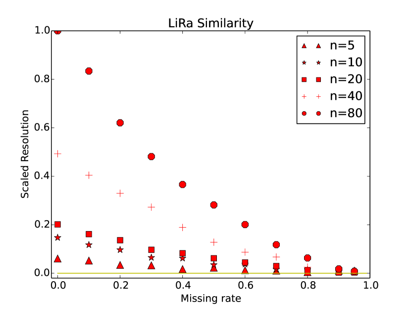
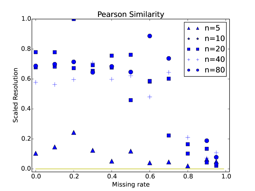
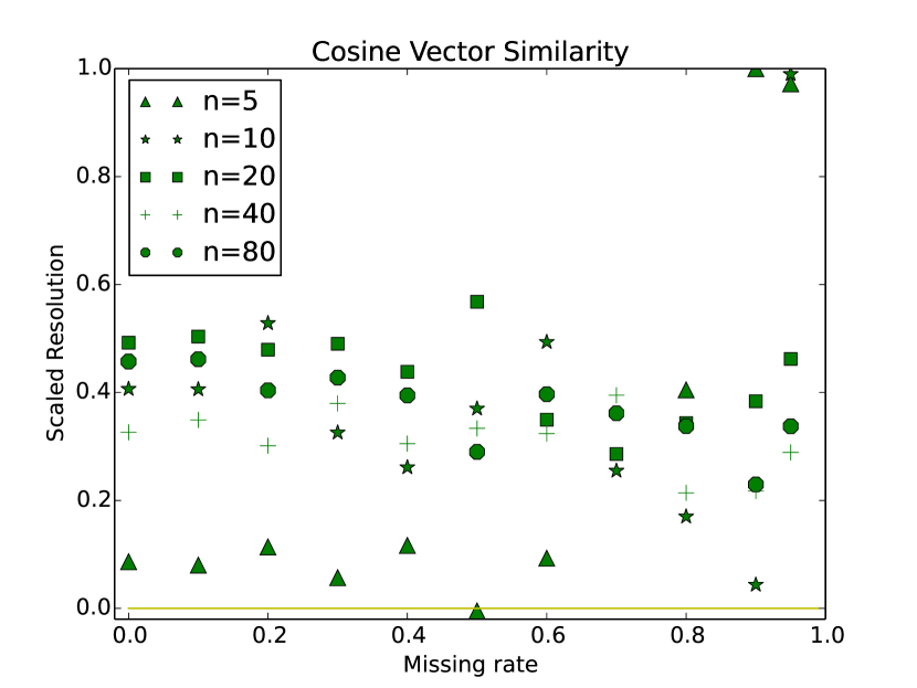
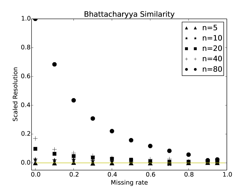
Figure 3: Similarity resolution (higher is better) as a function of missing data rate plotted for four similarity scores: LiRa (upper left), Pearson (upper right), Cosine (lower left), and Bhattacharyya (lower right). Resolution indicates a score’s ability to differentiate a pair of points in the same cluster from a pair of points in different clusters. Cosine and Pearson scores do not improve in resolution with more data availability.

We observe that the resolution of the LiRa score is greater as we decrease missing data and increase the dimensionality. In addition, the LiRa resolution is positive for all values of the missing rate and all dimensionalities (the minimum of LiRa resolutions was 0.051), indicating greater average intra- than inter-cluster LiRa similarity. The greater magnitude of the resolution in the presence of more data shows the ability of LiRa to make stronger claims about similarity as the number of co-observed entries in two discrete-valued vectors increases. More data comes in the form of a lower missing data rate, but also increased dimensionality, because there will be more expected co-observed entries between two vectors when the dimensionality is higher.

Contrast this with the Pearson and Cosine similarity scores, where dimensionality and missing data have virtually no effect on the resolution, except that high values of missing rates tend to lower the Pearson resolution dramatically. The resolution is positive for most values of the dimensionality and missing rates for Cosine, and all values of dimensionality and missing rates for Pearson, but increasing the amount available data does not improve the ability of Cosine or Pearson to resolve similar from dissimilar users. The fact that low dimensionalities and higher missing rates often yield a higher resolution than higher dimensionalities and lower missing rates shows theses scores’ inability to make use of more data for more accurate similarity judgments. For the most part, the Bhattacharyya resolution tends to increase with increasing dimensionality and decreasing missing rates, also indicating a greater difference between intra- and inter- cluster scores, but there are instances when this is not the case.

We conclude this section with a discussion of Figure 4, which plots the scaled average inter-cluster similarity score across missing rates for the four tested scores, with a fixed dimension of $n=80$. Scaling was again done by dividing each average inter-cluster similarity by the magnitude of the greatest-magnitude average inter-cluster similarity that occurred over all missing rates. This way, we can see how inter-cluster similarity changes with the missing rate, for all scores on the same scale.

Recall that a negative Pearson or LiRa value indicates dissimilarity in some way. A negative Pearson score indicates anti-correlated co-observed entries. A negative LiRa score indicates a greater chance that the data in co-observed entries was generated by chance, rather than that the data comes from two vectors in the same cluster. In Bhattacharyya, a negative score also indicates anti-correlation in the co-observed entries, but weighted by item similarity and shifted by the Jaccard similarity, making it harder to interpret. Cosine is restricted to positive values in this setting, because all vector entries were positive.

We observe that LiRa and Pearson appear to be better able to indicate dissimilarity, as their scaled average inter-cluster values are negative for most and all missing rates, respectively. However, LiRa again makes use of more data to make a stronger claim about dissimilarity, giving greater-magnitude negative values when more data is observed. Both Cosine and Bhattacharyya remain positive, indicating some similarity between points from different clusters, and actually increase in magnitude as more data becomes available, scoring two points from different clusters higher at lower missing rates. Based on the MovieLens results, this may also mean that the real data contains user clusters, and the Bhattacharyya score is too high for users from different clusters. Thus it may choose sub-optimal neighbors in the kNN method in this case.

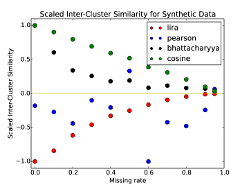
Figure 4: The inter-cluster similarity of various similarity scores on synthetic data. LiRa is the only score which decreases with decreasing missing rate, indicating greater ability to differentiate points from different clusters when more data is available.

Based on our results from these synthetic data experiments, we make two concluding remarks about the results on real data in Section 4.3. First, the high performance of LiRa on the MovieLens data can be explained by its dependence on not only the rating patterns in co-observed entries of user rating vectors, but also on the amount of data that is available to make the similarity computation. Second, based on the Bhattacharyya results, we believe a promising future research direction is to further investigate what type of underlying cluster structure exists in RS data. The intuition behind the Bhattacharyya similarity is that a higher similarity between two items in the set $I_{uv}$, defined by the difference between their rating distributions across the entire data set, should contribute a higher weight to the difference in these item ratings. Each of the $|I_{uv}|^{2}$ pairs of co-rated items $(i,j)$ contributes to the similarity score. By contrast, LiRa does not consider item similarity in the computation of user similarity, and only examines the differences in user ratings of the $|I_{uv}|$ co-rated items. A clustering structure such as that assumed by LiRa may indeed exist in real-world data, and perhaps the Bhattacharyya score is not well suited to this setting, where it can be high for users from different clusters, despite its ability to give greater scores to users from the same cluster with more data.

5 Related Work

Early studies  [18, 11, 8] consistently rate the Pearson, Cosine Vector, or slight variants as the superior similarity scores for RS data. Several recent studies [1, 16] focus on the cold start problem, in which extremely few ratings are available for a new user, making it difficult to determine her similarity to other users with traditional similarity scores.

The PIP heurisitic was introduced by Ahn [1] to address the cold-start problem, but was shown to perform comparably to traditional similarity scores such as Pearson’s correlation coefficient in non-cold start settings, and was outperformed in terms of rating prediction accuracy by the Bhattacharyya coefficient for collaborative filtering in cold start settings with extremely few ratings. Patra et al.’s Bhattacharyya coefficient for collaborative filtering, defined in Section 4, takes into account item similarity as a weighting scheme for user similarity. It was developed for the extremely sparse setting, thus Patra et al.’s empirical evaluation of its use in rating prediction accuracy is restricted to data sets where the missing rate is much higher than even the already sparse MovieLens datasets, and is better suited for the cold-start setting. The Bhattacharyya coefficient also is more computationally expensive than our LiRa score, as it requires all-to-all user-to-user as well as all-to-all item-to-item similarity computations.

In the context of statistical text analysis, Dunning [9] makes a strong case for the use of a log-likelihood ratio to examine the statistical significance of word or bigram frequencies in sparse data. The hypotheses in the LiRa ratio express whether users are or are not similar, based on the assumption that user similarity is reflected by the probability of two users’ ratings being distributed according to the clustering model presented in Section 3. These are different from the hypotheses of the dimensionality of the underlying parameter space as defined by Dunning. Dunning’s work has been adapted to RS data in several ways and has been shown to enhance the performance of recommender systems in an industrial setting [4, 15]. However, we emphasize that in the applied versions of Dunning’s likelihood ratio to RS data, the ratio is used either as a filter for finding relevant items to use in similarity computations, or a weighting term in the rating prediction phase, and has not been developed into a similarity score. Our method also slightly resembles Jojic et al.’s [13] item similarity score, where similarity is determined by comparing the number of users that like two items to the number expected by chance. However, their method is limited to binary like/dislike data, treats dislikes the same as missing entries in the item similarity computation, and was used in combination with additional heuristics to determine whether a user will like a particular item.

The intuition that inherent clusters of users exist in RS data has been explored by several clustering methods which were developed to improve prediction accuracy in RS data. Sarwar et al. [19] used clustering to improve scalability by first partitioning the users into clusters, then making a prediction based on averaging ratings from members of the same cluster, allowing for less computation time than a kNN method on the MoveLens 100K data set. Similarly, Xue et al. introduce a $k$-means clustering phase prior to prediction [20], and predict a rating for a user $u$ by choosing $k$ neighbors out of the clusters with representatives that score highly with $u$. Rashid et al. [2] incorporate bisecting $k$-means clustering “to increase efficiency and scalability while maintaining good recommendation quality" in their ClustKNN algorithm. Das et al. [7, 6] use a DBSCAN-based algorithm to improve kNN prediction accuracy. An extensive experimental study of the effectiveness of various centroid selection methods for the $k$-means algorithm when used as a pre-processing step in recommendation systems is presented by Zahra et al. [21], who conclude that although many approaches improve prediction accuracy and efficiency, no algorithm is “a panacea" across all data sets. Nonetheless, the results of clustering-based approaches in rating prediction are encouraging, as they show promise in improving both accuracy and scalability of recommender systems.

6 Conclusion

We have introduced the LiRa similarity score for discrete-valued, sparse, and high-dimensional data, typical of the RS domain. We have shown through empirical evaluations on both real and synthetic data that LiRa’s assumptions about a clustering model of users makes it a good indicator of user similarity, and that it outperforms other measures in this capacity. An exciting area to focus our future research is exploring how to devise a better model of clustering structure within RS data in order to improve prediction accuracy of collaborative filtering methods. Another possible research direction is to develop fast clustering methods that use LiRa as a similarity score to improve the scalability of user-based collaborative filtering.

References

- [1] H. J. Ahn. A new similarity measure for collaborative filtering to alleviate the new user cold-starting problem. Information Sciences, 178(1):37–51, 2008.
- [2] S. K. L. Al Mamunur Rashid, G. Karypis, and J. Riedl. Clustknn: a highly scalable hybrid model-& memory-based cf algorithm. Proceeding of WebKDD, 2006.
- [3] J. Bobadilla, F. Ortega, A. Hernando, and A. Gutiérrez. Recommender systems survey. Knowledge-Based Systems, 46:109–132, 2013.
- [4] P. Casinelli. Evaluating and implementing recommender systems as web services using apache mahout.
- [5] J. Cheema and J. Dicks. Computational approaches and software tools for genetic linkage map estimation in plants. Briefings in Bioinformatics, 10(6):595–608, 2009.
- [6] J. Das, S. Majumder, D. Dutta, and P. Gupta. Iterative use of weighted voronoi diagrams to improve scalability in recommender systems. In Advances in Knowledge Discovery and Data Mining, pages 605–617. Springer, 2015.
- [7] J. Das, P. Mukherjee, S. Majumder, and P. Gupta. Clustering-based recommender system using principles of voting theory. In Contemporary Computing and Informatics (IC3I), 2014 International Conference on, pages 230–235. IEEE, 2014.
- [8] C. Desrosiers and G. Karypis. A comprehensive survey of neighborhood-based recommendation methods. In Recommender systems handbook, pages 107–144. Springer, 2011.
- [9] T. Dunning. Accurate methods for the statistics of surprise and coincidence. Computational linguistics, 19(1):61–74, 1993.
- [10] A. Gunawardana and G. Shani. Evaluating recommender systems. In Recommender Systems Handbook, pages 265–308. Springer, 2015.
- [11] J. Herlocker, J. A. Konstan, and J. Riedl. An empirical analysis of design choices in neighborhood-based collaborative filtering algorithms. Information Retrieval, 5(4):287–310.
- [12] J. L. Herlocker, J. A. Konstan, L. G. Terveen, and J. T. Riedl. Evaluating collaborative filtering recommender systems. ACM Transactions on Information Systems (TOIS), 22(1):5–53, 2004.
- [13] O. Jojic, M. Shukla, and N. Bhosarekar. A probabilistic definition of item similarity. In Proceedings of the fifth ACM conference on Recommender systems, pages 229–236. ACM, 2011.
- [14] M. E. Newman. Modularity and community structure in networks. Proceedings of the national academy of sciences, 103(23):8577–8582, 2006.
- [15] D. Paraschakis, B. J. Nilsson, and J. Holländer. Comparative evaluation of top-n recommenders in e-commerce: an industrial perspective.
- [16] B. K. Patra, R. Launonen, V. Ollikainen, and S. Nandi. A new similarity measure using bhattacharyya coefficient for collaborative filtering in sparse data. Knowledge-Based Systems, 82:163–177, 2015.
- [17] F. Ricci, L. Rokach, and B. Shapira. Introduction to recommender systems handbook. Springer, 2011.
- [18] B. Sarwar, G. Karypis, J. Konstan, and J. Riedl. Item-based collaborative filtering recommendation algorithms. In Proceedings of the 10th international conference on World Wide Web, pages 285–295. ACM, 2001.
- [19] B. M. Sarwar, G. Karypis, J. Konstan, and J. Riedl. Recommender systems for large-scale e-commerce: Scalable neighborhood formation using clustering. In Proceedings of the fifth international conference on computer and information technology, volume 1. Citeseer, 2002.
- [20] G.-R. Xue, C. Lin, Q. Yang, W. Xi, H.-J. Zeng, Y. Yu, and Z. Chen. Scalable collaborative filtering using cluster-based smoothing. In Proceedings of the 28th annual international ACM SIGIR conference on Research and development in information retrieval, pages 114–121. ACM, 2005.
- [21] S. Zahra, M. A. Ghazanfar, A. Khalid, M. A. Azam, U. Naeem, and A. Prugel-Bennett. Novel centroid selection approaches for kmeans-clustering based recommender systems. Information Sciences, 2015.