Species substitution, graph suspension, and graded Hopf algebras of painted tree polytopes.

Abstract.

Combinatorial Hopf algebras of trees exemplify the connections between operads and bialgebras. Painted trees were introduced recently as examples of how graded Hopf operads can bequeath Hopf structures upon compositions of coalgebras. We put these trees in context by exhibiting them as the minimal elements of face posets of certain convex polytopes. The full face posets themselves often possess the structure of graded Hopf algebras (with one-sided unit). We can enumerate faces using the fact that they are structure types of substitutions of combinatorial species. Species considered here include ordered and unordered binary trees and ordered lists (labeled corollas). Some of the polytopes that constitute our main results are well known in other contexts. First we see the classical permutahedra, and then certain generalized permutahedra: specifically the graph-associahedra of suspensions of certain simple graphs. As an aside we show that the stellohedra also appear as liftings of generalized permutahedra: graph composihedra for complete graphs. Thus our results give examples of Hopf algebras of tubings and marked tubings of graphs. We also show an alternative associative algebra structure on the graph tubings of star graphs.

1. Introduction

The mathematical operation of grafting trees, root to leaf, is a key feature in the structure of several important operads and Hopf algebras. Loday and Ronco initiated the study of these type of structures when they found a Hopf algebra of plane binary trees in [18]. The Loday-Ronco algebra is based on the vertices of Stasheff’s associahedra, the polytopes that model homotopy associative spaces.

There is a surjection from permutations to plane binary trees: the Tonks projection, defined in [27], from the permutohedron to the associahedron. Chapoton found that the Hopf algebras of vertices of these polytopes are subalgebras of larger ones based on the faces of the respective polytopes [8]. Chapoton’s algebras are the differential graded structures corresponding to algebras described by Loday and Ronco in [20]. Using that same surjection on basis elements, the Loday-Ronco algebra is the image of the Malvenuto-Reutenauer Hopf algebra of permutations [21]. There is also a projection from the Loday-Ronco Hopf algebra to the algebra of quasisymmetric polynomials. The authors of [18] showed Hopf algebra maps which factor the descent map from permutations to Boolean subsets.

In [19] the authors describe the product of planar binary trees in terms of the Tamari order. In 2005 and 2006 Aguiar and Sottile characterized operations in these algebras by using Möbius functions (of the Tamari order and of the weak Bruhat order) to obtain new bases, in respectively [2],[1]. Their work gave a nice way to construct a basis of primitive elements, using the irreducible trees. In [17] the authors characterize the same operations in terms of inclusions (into the larger polytopes) of products of polytope faces.

Alternatively, since the Loday-Ronco algebra is self-dual, it can project to the divided power Hopf algebra. In [15] the authors used the following notation: $\mathfrak{S}Sym$ for the Malvenuto-Reutenauer Hopf algebra, $\mathcal{Y}Sym$ for the Loday-Ronco Hopf algebra, and $\mathfrak{C}Sym$ for the divided power Hopf algebra. They defined the idea of grafting with two colors, preserving the colors after the graft in order to have two-tone, or painted, trees with various structures possible in each colored region. Here we review the definitions, adding some generality and defining poset structures on each set of painted trees. We extend the coalgebra structure to twelve new vector spaces, and we extend the Hopf algbra structure to nine of those. We are also able to conclude that eight of the new coalgebras defined have underlying geometries of polytope sequences.

The stellohedra, or star-graph-associahedra, were first defined using the latter terminology by Carr and Devadoss in [7]. The former terminology was introduced in [24], where these polytopes were studied as special cases of nestohedra. In [14] the 3-dimensional version of the stellohedron appears graphically, as the domain and range quotient of the multiplihedra for the complete graphs. These quotients are the composihedra and cubeahedra respectively, but this source does not identify them as stellohedra. Also in [14] it is claimed without proof that grafted trees represent these quotients in all dimensions, although the corresponding trees in that source are associated in error to the wrong polytope. (We correct the mistake here; compare our Figures 4 and 4.3 to Figures 3 and 4 of [14].)

In [22] the authors do actually prove that the stellohedra for all dimensions are in fact the cubeahedra of complete graphs (which we will review). Also in [22] the stellohedron of dimension $n$ is recognized as the secondary polytope of pairs of nested concentric $n$-dimensional simplices. The stellohedra have also been seen as special cases of signed-tree associahedra in [23].

1.1. Main Results

Our algebraic results are twelve new graded coalgebras of painted trees, as described in Theorem 3.1. Nine of those contain as subalgebras the cofree graded coalgebras defined in [15], shown here in Figure 3. Eight of our new coalgebras also possess new one-sided Hopf algebra structures, some in multiple ways, as seen in Theorem 3.5. See Table 1 for reference. Eleven of these new coalgebras are based on the structure types of substitutions (partitional compositions) of species: nine seen in Theorem 3.6 (and the last two by bijection), leaving only one example without a way to calculate numbers of faces. For instance, the composihedra faces are counted by the ordinary generating function

$$(Y\circ L_{+}\circ L_{+})(x)=\frac{2x}{1-x+\sqrt{1-10x+17x^{2}}}$$

$$=x+3x^{2}+11x^{3}+49x^{4}+253x^{5}+1439x^{6}+\dots.$$

$C=$	$D=$	New	New	Face	Composition	Tubings	Lifted
rooted	rooted	graded	Hopf	poset of	(Substitution)	of Graph	Gen.
forests	trees	Coalgebra	Algebra	polytopes	of Species	Suspension	Perm.
Corollas	Corollas	x	x	x	x		x
	Plane	x	x	x	x		x
	Weak order	x	x	x	x	x	x
Plane	Corollas	x	x	x	x		x
trees	Plane	x	x	x	x		x
	Weak order	x	x	x	x	x	x
Weakly	Corollas	x	x	conj.	x
ordered	Plane	x	x	conj.	x
trees	Weak order	x	conj.	conj.	x
Weakly	Corollas	x	x	x	x	x	x
ordered	Plane	x	conj.	conj.
forest	Weak order	x	conj.	x	x	x	x

Table 1. Summary of known results about the sets $\widetilde{C/D}$, organized by tree types as seen in Figure 4.

We show that eight sequences of our 12 sets of painted trees, with defined relations, are isomorphic as posets to face lattices of convex polytopes. Six of these are in the collection of Hopf algebras just mentioned. Four of these isomorphisms are well known from previous work: the associahedra, multiplihedra, composihedra and cubes. Four of our new coalgebras are based on tubings of suspensions of simple graphs. In Theorem 4.11 we show that weakly ordered forests grafted to weakly ordered trees are isomorphic to the permutohedra. In Theorem 4.12 we show that forests of corollas grafted to weakly ordered trees are isomorphic to the star-graph-associahedra, or stellohedra. In Theorem 4.14 and Theorem 4.15 we show that weakly ordered forests grafted to a corolla are also isomorphic to stellohedra. In Theorem  4.16 we show that forests of plane trees grafted to weakly ordered trees are isomorphic to the fan-graph-associahedra, or pterahedra. In Theorem 4.13 we show that the stellohedra again appear as graph-composihedra for the complete graphs.

In Section 2 we define the sets of trees and the surjective functions between those sets. In Section 3 we define the operations on our trees and explain which sets are graded coalgebras and which are Hopf algebras. We give examples of products, coproducts, and antipodes.

In Section 4 we define a partial ordering of painted trees and show which of our posets of trees represent combinatorial equivalence classes of polytopes. In Section 5 we describe our Hopf algebra of faces of the stellohedra using graph tubings. In Proposition 6.3 we show that a new, less forgetful, product on vertices of the stellohedra is associative.

2. Definitions

Graphs with unlabeled vertices are isomorphism classes of graphs. In this paper, trees are unlabeled, connected, acyclic, simple graphs. A rooted tree is an oriented tree having one maximal vertex or node, called the root. For any node $v$ of a tree, the edges oriented towards $v$ are called inputs of $v$ and the edges leaving from $v$ are called outputs of $v$. We denote by ${\mbox{In}(v)}$ the set of inputs of $v$, and by ${\mbox{Out}(v)}$ the set of outputs of $v$.

We denote by ${\mbox{Nod}(t)}$ the set of nodes of a tree $t$. All the trees we work with satisfy that $|{\mbox{In}(v)}|>1$ and $|{\mbox{Out}(v)}|=1$. We admit edges which are linked to a unique node, one of them is the output of the root, the others are called leaves. The degree of a tree is the number of its leaves minus $1$.

We use the following terms:

• A plane tree is a rooted tree satisfying that the set ${\mbox{In}(v)}$ is totally ordered, for any node $v$. Sometimes this is also referred to as planar, and can be equivalently satisfied by requiring the leaves to lie in one horizontal line, in order, and the root at a lesser $y$-value.

• A binary tree is a rooted tree such that $|{\mbox{In}(v)}|=2$, for any node $v$.

An example of plane rooted binary tree, often called a binary tree when the context is clear, is the following, where the orientation of edges is higher to lower on the plane:

The leaves are ordered left to right as shown by the circled labels. The horizontal node ordering corresponds to the order of gaps between leaves: the $n^{th}$ gap is just to the left of the $n^{th}$ leaf and the $n^{th}$ node is the one where a raindrop would be caught which fell in the $n^{th}$ gap. This ordering is also described as a depth first traversal of the nodes. Non-leafed edges are referred to as internal edges. The set of plane rooted binary trees with $n$ nodes and $n+1$ leaves is denoted $\mathcal{Y}_{n}.$ The cardinality of these sets are the Catalan numbers:

$$|\mathcal{Y}_{n}|=\frac{1}{n+1}{2n\choose n}.$$

We will also need to consider rooted plane trees whose vertices, or nodes, have more than two inputs. We denote by ${\mathcal{T}}_{n}$ the set of all plane rooted trees with $n+1$ leaves. The cardinal of ${\mathcal{T}}_{n}$ is the $n^{th}$ super-Catalan number (also called the little Schröder number).

An $(n+1)$-leaved rooted tree with only one node (it will have degree $n+2\geq 3$), or, for $n=0,$ a single leaf tree with zero nodes, is called a corolla, denoted $\mathfrak{C}_{n}.$ This notation for the (set of one) corolla with $n+1$ leaves is the same as used for the set of one left comb in [15]. In the current paper we have decided that the corollas are more easily recognized than the combs.

2.1. Ordered and painted plane trees

Many variations of the idea of the plane tree have proven useful in applications to algebra and topology.

Notation 2.2.

For any positive integer $n\geq 1$, we denote by $[n]$ the ordered set $\{1,2,\dots,n\}$, and by $[n]_{0}$ the set $\{0\}\cup[n]$.

Definition 2.1.

An ordered tree (sometimes called leveled) is a plane rooted tree $t$, equipped with a vertical linear ordering of ${\mbox{Nod}(t)}$, in addition to the horizontal one. That is, an ordered tree is a plane rooted tree $t$ equipped with a bijective map $L:{\mbox{Nod}(t)}\longrightarrow[|{\mbox{Nod}(t)}|]$, which respects the order given by the vertical order. Clearly $L({\mbox{root}})=|{\mbox{Nod}(t)}|$.

This vertical linear ordering extends the partial vertical ordering given by distance from the root. This vertical ordering allows a well-known bijection between the ordered trees with $n$ nodes, denoted $\mathfrak{S}_{n},$ and the permutations on $[n].$

We may draw an ordered tree in three different styles:

The corresponding permutation in the above picture is $\sigma=(3,2,4,1)$, in the notation $(\sigma(1),\sigma(2),\sigma(3),\sigma(4).)$

We will also consider forests of trees. In this paper, all forests will be a linearly ordered list of trees, drawn left to right. This linear ordering can also be seen as an ordering of all the nodes of the forest, left to right. On top of that, we can also order all the nodes of the forest vertically, giving a vertically ordered forest, which we often shorten to ordered forest. This initially gives us four sorts of forests to consider, shown in Figure 1.

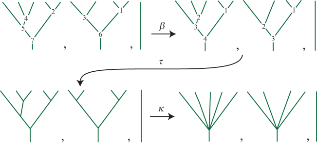
Figure 1. Following the arrows: a (vertically) ordered forest, a forest of ordered trees, a forest of binary trees, and a forest of corollas.

Also shown in Figure 1 are three canonical, forgetful maps between the types of forests.

Definition 2.2.

We define $\beta$ to be the function that takes an ordered forest $F$ and gives a forest of ordered trees. The output $\beta(F)$ will have the same list of trees as $F$, and for a tree $t$ in $\beta(F)$ the vertical order of the nodes of $t$ will respect the vertical order of the nodes in $F.$ That is, for two nodes $a,b$ of $t$ we have $a\leq b$ in $t$ iff $a\leq b$ in $F.$

We define $\tau$ to be the function that takes an ordered tree and outputs the tree itself, forgetting all of the vertical ordering of nodes (except for the partial ordering based on distance from the root.) We define $\kappa$ to be the function that takes a tree and gives the corolla with the same number of leaves.

Note that $\tau$ and $\kappa$ are immediately both functions on forests, simply by applying them to each tree in turn. Also note that $\tau$ and $\kappa$ are described in [15], but that there $\kappa$ yields a left comb rather than a corolla.

Now we define larger sets of trees that generalize the binary ones. First we drop the word binary; we will consider plane rooted trees with nodes that have any degree larger than two. Then, from the non-binary vertically ordered trees we further generalize by allowing more than one node to reside at a given level. Instead of corresponding to a permutation, or total ordering, these trees will correspond to an ordered partition, or weak ordering, of their nodes.

Definition 2.3.

A weakly ordered tree is a plane rooted tree with a weak ordering of its nodes that respects the partial order of proximity to the root.

Recall that this means all sets of nodes are comparable–but some are considered as tied when compared, forming a block in an ordered partition of the nodes. The linear ordering of the blocks of the partition respects the partial order of nodes given by paths to the root.

For a weakly ordered tree with $n+1$ leaves the ordered partition of the nodes determines an ordered partition of $S=\{1,\dots,n\}$, as described in [27]. Here we see $S$ as the set of gaps between leaves. (Recall that a gap between two adjacent leaves corresponds to the node where a raindrop would eventually come to rest; $S$ is partitioned into the subsets of gaps that all correspond to nodes at a given level.) Weakly ordered trees are drawn using nodes with degree greater than two, and using numbers and dotted lines to show levels.

The ordered partition corresponding to the above pictures is $(\{2,5\},\{1\},\{3,4\}).$ Note that an ordered tree is a (special) weakly ordered tree.

As well as forests of weakly ordered trees we also consider weakly ordered forests. This gives us three more sorts of forests to consider, shown in Figure 2. As indicated in that figure, the maps $\beta,\tau$ and $\kappa$ are easily extended to forests of the non-binary and/or weakly ordered trees: $\beta$ forgets the weak ordering of the forest to create a forest of weakly ordered trees, $\tau$ forgets the weak ordering, and $\kappa$ forgets the partial order to create corollas.

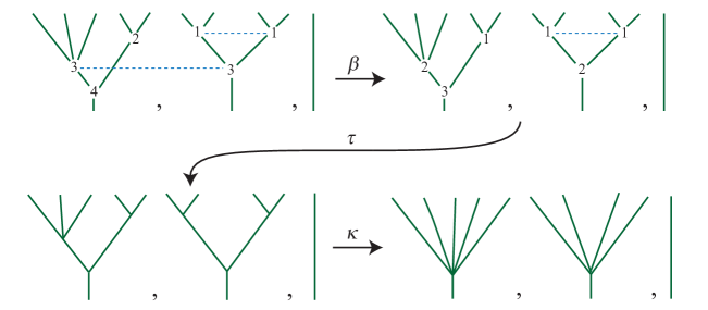
Figure 2. Following the arrows: a (vertically) weakly ordered forest, a forest of weakly ordered trees, a forest of plane rooted trees, and a forest of corollas. Note that the forests in Figure 1 are special cases of these.

The trees we focus on in this paper generalize those introduced in [15]. They are constructed by grafting together combinations of ordered trees, binary trees, and corollas. Visually, this is accomplished by attaching the roots of one of the above forests $w\in C$ to the leaves of one of the above types of trees $v\in D$, but remembering the originals $w$ and $v$. The result is denoted $w/v\in C/D.$ We use two colors, which we refer to as “painted” and “unpainted.” The forest is described as unpainted, and the base tree (which the forest is grafted to) is painted. At a graft the leaf is identified with the root, and in the diagram that point is no longer considered a node, but is rather drawn as a change in color (and thickness, for easy recognition) of the resulting edge. (Note that in some papers such as [13] our mid-edge change in color is described instead as a new node of degree two.)

With regard to the partial ordering of nodes by proximity to the root (with the closest to the root being least), we can describe a painted tree as having a distinguished order ideal of painted nodes.

We refer to the result as a (partly) painted tree, regardless of the types of upper (unpainted) and lower (painted) portions. Notice that in a painted tree the original trees (before the graft) are still easily observed since the coloring creates a boundary, called the paint-line halfway up the edges where the graft was performed. Thus the paint line separates the painted tree into a single tree of one color and a forest of trees of another color. In Figure 3 we show all 12 ways to graft one of our types of partially ordered forest with one of our types of tree.

Definition 2.4.

The maps $\beta,\tau$ and $\kappa$ are now extended to the painted trees, just by applying them to the unpainted forest and/or to the painted tree beneath. We indicate this by writing a fraction: $\displaystyle{\frac{f}{g}}$ for two of our three maps, or the identity map, as seen in Figure 3. That is, $\displaystyle{\frac{f}{g}}$ indicates applying $f$ to the forest and $g$ to the painted base tree, for $f,g\in\{\beta,\tau,\kappa,1\}$.

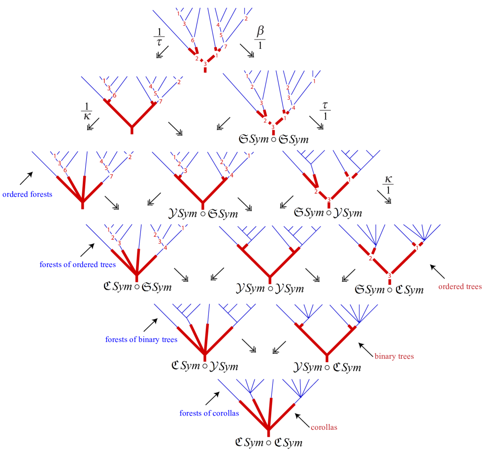
Figure 3. Varieties of grafted, painted trees. Each diagonal shares a type of tree on the bottom (painted) or a type of forest grafted on, as indicated by the labels. Nine are labeled with the compositions of coalgebras from [15]. Trees in this figure correspond to vertex labels of the 10-dimensional polytopes in sequences whose 3-dimensional versions are shown in Example 4.3. The forgetful maps are shown with example input and output. Parallel arrows all denote the same map, except of course that the identity is context dependent.

2.3. General painted trees.

Now our definition of painted trees is expanded to include any of our types of forest grafted to any of our types of tree. On top of that we will also permit a further broadening of the allowed structure of our painted trees. The paint-line, where the graft occurs, is allowed to coincide with nodes, where branching occurs. We call it a half-painted node. In terms of the grafting of a forest onto a tree our description depends on the type of forest. If the forest is weakly ordered, or is a forest of weakly ordered trees, then we see each half-painted node as grafting on a single tree at its least node, after removing its trunk and root. If the forest is only partially ordered (i.e. of binary trees or corollas) then we see the half-painted nodes as (possibly) several roots of several trees simultaneously grafted to a given leaf. For a choice $C$ of forests and a choice $D$ of trees, the resulting general trees are denoted $\widetilde{C/D}.$ See the examples in Figures 4 and 5.

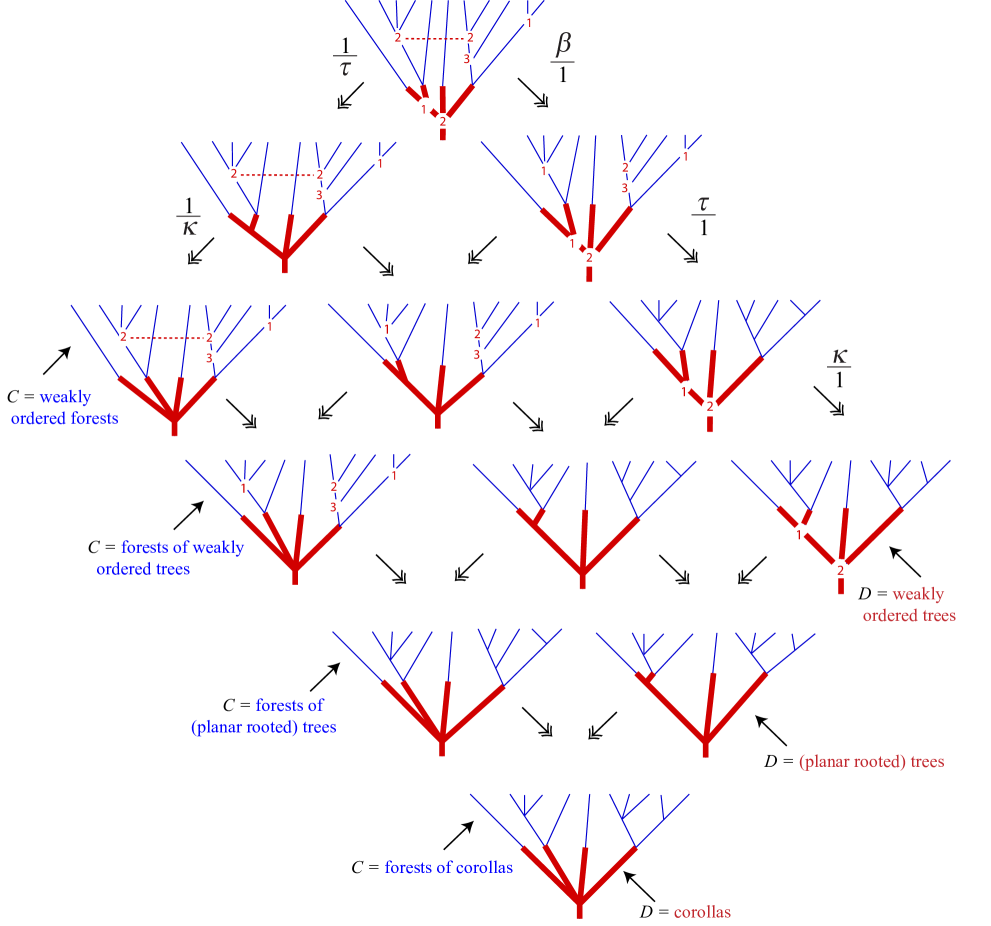
Figure 4. General varieties of grafted, painted trees $\widetilde{C/D}$. For those proven to be polytopes in Section 4, these correspond to face labels of the 10-dimensional polytope sequences whose 3-dimensional versions are shown in Example 4.3. Parallel arrows all denote the same map. Note that the trees in Figure 3 are special cases—vertex trees, or minimal in the face lattice—of the types illustrated in this figure.

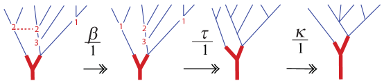
Figure 5. Action of the projections, detail from Figure 4. At first on the left there is a weakly ordered forest. Then there are weakly ordered trees, one attached at each half-painted node. Next there are two or three plane trees attached at the paint line; we can see the righthand half painted node as incident with either one or two trees without any contradiction. Finally there is a forest of 3 separate corollas.

For these general painted trees we can again extend the “fractional” maps using $\beta,\tau$ and $\kappa.$ We reiterate from above how the half-painted nodes are interpreted, since that determines the input for the “numerator” map. Specifically $\displaystyle{\frac{\beta}{g}}$ operates by taking as input for $\beta$ the weakly ordered forest of trees, one tree for each half-painted node. That is, $\displaystyle{\frac{\beta}{g}}$ treats the half-painted nodes as being the location of a single tree that is grafted on without a trunk. This description is the same for $\displaystyle{\frac{\tau}{g}}.$ In contrast however, the map $\displaystyle{\frac{\kappa}{g}}$ takes as input the forest found by listing all the unpainted trees while assuming each has a visible trunk, some of which are simultaneously grafted at the same half-painted node. Examples of these maps are shown in Figure 4, where we show 12 general painted trees that consist of one of the four general types of forest and one of the three general types of trees. Figure 5 is a detail from Figure 4 showing how the actions of the projections differ.

3. Hopf Algebras

Let ${\mathbb{K}}$ denote a field. For any set $X$, we denote by ${\mathbb{K}}[X]$ the ${\mathbb{K}}$-vector space spanned by $X$. As in [15] we work over a fixed field of characteristic zero, and our vector spaces will be constructed by using the sets of trees as graded bases.

Recall from [15] the concept of splitting a tree, given a multiset of its leaves. Here, modified from an example in [14], is a 4-fold splitting into an ordered list of 5 trees:

Also recall the process of grafting an ordered forest to the leaves of a tree:

In [15] there are defined coproducts on nine of the families of painted trees shown in Figure 3 (the ones with labels denoting their membership in a composition of coalgebras). Eight of these, all but the composition of coalgebras $\mathfrak{S}\mathit{Sym}\circ\mathfrak{S}\mathit{Sym}$, are shown to possess various Hopf algebraic structures in [15]. Now we show which of those structures can be extended to our generalized painted trees in Figure 4.

The Hopf algebras we are interested in first are the algebra of corollas, called $\mathfrak{C}Sym$ and shown to be identical to the divided power Hopf algebra in [15]; second the algebra of rooted planar binary trees $\mathcal{Y}Sym$ which is known as the Loday-Ronco Hopf algebra, and finally the algebra of rooted planar trees $\mathcal{Y}\widetilde{Sym}.$ The latter is the Hopf algebra of faces of the associahedra as described in [8], and in terms of graph tubings in [17].

The coproducts and products are all defined in [15] using subscripts: the element of the vector space is $F_{w}$ where $w$ is a tree of the given type. The coproduct is defined by splitting:

$$\Delta(F_{w})=\sum_{w\stackrel{{\scriptstyle\curlyvee}}{{\to}}(w_{0},w_{1})}F_{w_{0}}\otimes F_{w_{1}},$$

where the sum is over all ways to split the tree $w$ at one leaf; so has $n$ terms. Multiplication on the left is defined by splitting the left operand and grafting to the right operand:

$$F_{w}\cdot F_{v}=\sum_{w\stackrel{{\scriptstyle\curlyvee}}{{\to}}(w_{0},\dots,w_{n})}F_{(w_{0},\dots,w_{n})/v},$$

where the sum is over all ways to split the tree $w$ at a multiset of $n-1$ leaves (where $n$ is the number of leaves of $v.$)

We will often eliminate the subscript notation and simply draw the basis element. For example, here is the coproduct in $\mathcal{Y}Sym$:

Here is how to multiply two trees in $\mathcal{Y}Sym$:

For more examples see [15].

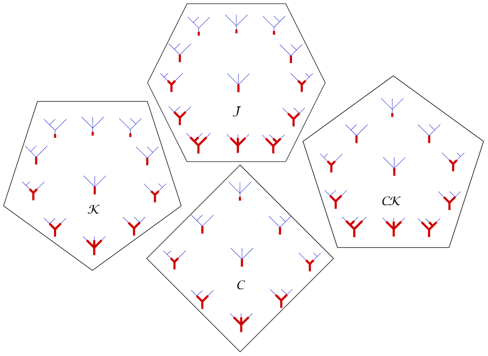
Figure 7. These are the 2-dimensional terms with their faces labeled. The same labels are used no matter where the shape occurs in figure 6.

Given any of the 12 types of painted tree from Figure 4, we get a graded vector space where trees with $n$ leaves comprise the basis of degree $n-1.$ The basis of degree 0 is the single-leaved painted tree–this is the same for each of the 12 cases. The degree 1 basis is also identical for all 12 cases: the three painted trees with 2 leaves. The 12 cases differ when it comes to the degree 2 bases, as seen in Figure 7. Note that while most of the trees in Figure 3 can be seen as coming from a composition of coalgebras, as labeled, the general trees in Figure 4 cannot since the unpainted forests can be grafted in multiple ways. However, they can often still possess a coproduct, given by splitting the trees leaf to root. Splitting a tree of a given type always produces two trees of that same type. The weakly ordered trees and weakly ordered forests can be split into two weakly ordered trees or forests. In fact we have the following:

Theorem 3.1.

The action of splitting trees leaf to root makes each of the tree types in Figure 4 into the basis of a graded coassociative coalgebra.

Proof.

The coproduct of a basis element is the sum of pairs of trees which are formed by splitting at each leaf. Note that the degrees of the pairs each sum to $n-1.$ Coassociativity is seen by comparing both orders of applying the coproduct to the result of choosing any two leaves at which to split at the same time:

$$(\Delta\otimes 1)(\Delta(F_{w}))=(1\otimes\Delta)(\Delta(F_{w}))=\sum_{w\stackrel{{\scriptstyle\curlyvee}}{{\to}}(w_{0},w_{1},w_{2})}F_{w_{0}}\otimes F_{w_{1}}\otimes F_{w_{2}}.$$

∎

The compositions of coalgebras labeled in Figure 3 are subcoalgebras of the corresponding generalizations in Figure 4. We will denote these larger coalgebras by ${\mathcal{E}}=\widetilde{C/D}$ where $C$ and $D$ are the corresponding sets of trees. For example here is a coproduct in $\widetilde{C/D};$ in this picture the painted trees could be any of our twelve varieties.

Next we point out the actions of certain Hopf algebras on many of our coalgebras of generalized painted trees.

3.1. Hopf algebra modules

Using the same operations of splitting and grafting, we can often show that the Hopf algebras ${\mathcal{D}}=\mathcal{Y}S\widetilde{ym},$ and ${\mathcal{D}}=\mathfrak{C}\mathit{Sym}$ possess actions on painted trees which make our coalgebras of the latter into ${\mathcal{D}}$-modules.

Theorem 3.2.

For each ${\mathcal{E}}=\widetilde{C/D}$ with $C$ being the planar trees or corollas, the coalgebra ${\mathcal{E}}$ with basis $C/D$ is respectively a ${\mathcal{D}}=\mathcal{Y}S\widetilde{ym}$-module coalgebra or ${\mathcal{D}}=\mathfrak{C}\mathit{Sym}$-module coalgebra.

Proof.

We show that ${\mathcal{E}}$ is an associative left module, and that the action of ${\mathcal{D}}$ (denoted $\star$) commutes with the coproducts as follows: $\Delta_{\mathcal{E}}(d\star e)=\Delta_{\mathcal{D}}(d)\star\Delta_{\mathcal{E}}(e).$ We consider the action on basis elements. The action of a planar tree $d\in\mathcal{Y}S\widetilde{ym}$ (or corolla in $\mathfrak{C}\mathit{Sym}$ respectively) on a painted tree $e$ involves splitting $d$ and grafting the resulting forest onto the leaves of $e$. In the case of $C$ being corollas, the result of the grafting is then subjected to the application of $\kappa/1.$ Note that this application of $\kappa$ is equivalent to the composition in the operad of corollas, as pointed out in [15]. For example, where $C$ is the set of corollas:

Note in the above example that six terms result from choosing any two splits of the three leaves in the corolla. After applying $\kappa,$ there are duplicates as enumerated by the coefficients.

The associativity of the action is then straightforward to show on basis elements: given three layers of trees (the bottom layer is the painted tree) the result does not depend upon the order in which one makes the grafts.

The commutativity property is also straightforward on basis elements. Recall that the coproduct is applied linearly to each term in a sum, on the left side of the equation: $\Delta_{\mathcal{E}}(d\star e)$. Also recall that the action of a tensor product on a tensor product is performed componentwise: $(x\otimes y)\star(z\otimes w)=(x\star z)\otimes(y\star w)$ on the right side. Thus each term on the left-hand side is a pair of painted trees, formed by splitting after grafting a splitting of $d$ onto $e$. That pair is found on the right-hand side: all the splits are just performed before the grafting occurs. See the following example, where we pick out the matching terms.

∎

Theorem 3.3.

For each ${\mathcal{E}}=\widetilde{C/D}$ for $D$ being the planar trees or corollas, and $C$ being either corollas, planar trees, or weakly ordered trees, the coalgebra ${\mathcal{E}}$ with basis $C/D$ is respectively a ${\mathcal{D}}=\mathcal{Y}S\widetilde{ym}$-module coalgebra or ${\mathcal{D}}=\mathfrak{C}\mathit{Sym}$-module coalgebra.

Proof.

The same features need to be checked as in the proof of the previous theorem, which is straightforward. Now however the action of the Hopf algebra is on the right, so the product $e\star d$ involves splitting $e\in{\mathcal{E}}$ and then grafting to $d\in{\mathcal{D}}.$ ∎

The fact that one sided Hopf algebras exist for the generalized painted trees follows from the use of the maps $\beta,\tau,$ and $\kappa$ defined on trees and forests. We recall the definition of the sort of map we need from [15]. We let ${\mathcal{D}}$ be one of our connected graded Hopf algebras with product $v\cdot w.$

Definition 3.4.

A map $f:{\mathcal{E}}\to{\mathcal{D}}$ of connected graded coalgebras is a connection on ${\mathcal{D}}$ if ${\mathcal{E}}$ is a left (right) ${\mathcal{D}}$-module coalgebra and $f$ is both a coalgebra map and a module map:

$$(f\otimes f)\Delta_{\mathcal{E}}(e)=\Delta_{\mathcal{D}}f(e)~{}~{}and~{}~{}f(d\star e)=d\cdot f(e).$$

We have examples of connections $f$ using the maps $\tau$ and $\kappa$. If the target is corollas, we apply first $\tau$ and then $\kappa$ to a painted tree $w$. Then we forget the painting and apply $\kappa$ once more. The result is just a corolla with the same number of leaves as $w.$ If the target is planar trees we apply $\tau$ only, and then forget the painting. The result is a planar tree with the same branching structure as $w.$ These example connections are seen to be coalgebra and module maps by inspecting their action on basis elements: the result is the same if $f$ is applied before or after splitting and grafting.

Here is an example connection from planar trees over weakly ordered trees to planar trees:

Here is an example connection from corollas over weakly ordered trees to corollas:

Here is an example connection from corollas over planar trees to planar trees:

Theorem 3.5.

Consider the coalgebras ${\mathcal{E}}$ with graded bases the painted trees $C/D$ with $C$ (top) consisting of forests of planar trees or forests of corollas; and those with $D$ being planar trees or corollas (bottom) and with forests of planar trees, corollas or weakly ordered trees on top. Each of these eight coalgebras are one-sided Hopf algebras (they possess a one-sided unit and one-sided antipode.)

Proof.

We rely on Theorem 4.1 of [15], which states that when there is a connection $f:{\mathcal{E}}\to{\mathcal{D}}$ then ${\mathcal{E}}$ is a Hopf module and a comodule algebra over ${\mathcal{D}},$ and also a one-sided Hopf algebra in its own right. For those coalgebras $\widetilde{C/D}$ with planar trees or corollas on top (as $C$), the connection $f$ is the map to $C,$ the planar trees or corollas respectively. Note that in this case the product $\cdot:{\mathcal{E}}\otimes{\mathcal{E}}\to{\mathcal{E}}$ will be on the left: for $e,e^{\prime}\in{\mathcal{E}}$ we have, from the proof of Theorem 4.1 of [15], that $e\cdot e^{\prime}=f(e)\star e^{\prime}.$

For those coalgebras $\widetilde{C/D}$ with planar trees or corollas on bottom (as $D$), the connection $f$ is the map to $D,$ the planar trees or corollas respectively. Note that in this case the product $\cdot:{\mathcal{E}}\otimes{\mathcal{E}}\to{\mathcal{E}}$ will be on the right: for $e,e^{\prime}\in{\mathcal{E}}$ we have, from the proof of Theorem 4.1 of [15], that $e\cdot e^{\prime}=e\star f(e^{\prime}).$

We note that the one-sided unit $\eta=\eta(1)$ for either left or right products is the painted corolla with one leaf. The counit $\epsilon$ is a projection from ${\mathcal{E}}$ onto the base field: its value is the coefficient of the painted corolla with one leaf. ∎

Notice that some of our structures (the four painted trees that use no ordered trees) are Hopf algebras in two different ways. One has a left-sided unit and the other has a right-sided unit. Here is an example of the product in the Hopf algebra with left-side unit on the coalgebra $\widetilde{C/C}$ for $C$ the binary trees:

Here is an example of the product in the Hopf algebra with right-side unit on the coalgebra $\widetilde{C/C}$ for $C$ the binary trees:

Finally, we exhibit some antipodes $S:\widetilde{C/D}\to\widetilde{C/D}$. These are guaranteed to exist in connected graded bialgebras. For example, for left multiplication, the left antipode may be calculated with the recursive formula developed in [15], section 4:

$$S(\eta)=\eta;~{}~{}~{}~{}~{}~{}~{}~{}~{}~{}~{}~{}~{}~{}~{}~{}~{}~{}~{}S(e)=-\eta\cdot e-\sum S(e_{1})\cdot e_{2}$$

where the sum is over all splittings of $e$ into two painted trees $e_{1}$ and $e_{2}$, both with more than a single leaf.

Here are some examples, where the antipodes of larger trees can be found recursively using antipodes of their splittings:

3.2. Enumeration using species composition

Next we calculate the graded dimensions $d_{n}=$ dim$(\widetilde{C/D})_{n}$. For each coalgebra $\widetilde{C/D}$ this dimension is the sequence of numbers of basis elements. We find generating functions for the sequences of cardinalities of sets of trees, for most of the 12 tree varieties. In each case we want to count the trees themselves, but achieve this by finding the cardinality of a species $G$ which has structures those trees with labeled leaves. Recall that the set of structure types of a species is the collection of unlabeled versions of the combinatorial objects, as described in [5]. That source is also our reference for species substitution, also known as (partitional) composition.

However, since $n$ labels are assigned to the $n$ leaves in a row left to right, counting the number of structures of one of our species $G$ just means overcounting the structure types by a factor of $n!$. Thus the exponential generating function $\sum|G(n)|x^{n}/n!$ of the species is the same as the ordinary generating function of the graded dimension: $\sum d_{n}x^{n}.$ Note that for a given type of tree, the graded dimension is also the numbers of faces of the polytopes in the sequence, plus one for the polytope itself. The first few numbers in each sequence can be checked by hand-counting the faces in Example 4.3 and Figure 7.

Consider the combinatorial species $L_{+}$ of non-empty lists, $F$ of weakly ordered trees with labeled leaves, and $Y$ of plane rooted trees with labeled leaves. The exponential generating functions of two of these have nice closed forms: they are $\displaystyle{L_{+}(x)=\frac{x}{1-x},}$ whose derivatives at 0 give the factorials; and

$${Y(x)=\frac{2x}{1+x+\sqrt{1-6x+x^{2}}},}$$

whose derivatives at 0 give the super-Catalan numbers (numbers of faces of associahedra, A001003).

For the species $F$ of weakly ordered trees with $n$ labeled leaves, the structure types are counted by the Fubini numbers $f(n-1)$, since the number of gaps between leaves is $n-1.$ We are forced to use the exponential generating function:

$$F(x)=\sum_{n=1}^{\infty}f(n-1)x^{n}=x+x^{2}+3x^{3}+13x^{4}+75x^{5}+\dots$$

Notice that $F(x)$ is an exponential generating function for the series $n!f(n-1),$ which is the sequence counting the number of ordered trees with $n$ labeled leaves.

Now we are able to set up ordinary generating functions for the sets $\widetilde{C/D},$ for the cases in which $\widetilde{C/D}$ is describable as the structure types of a composition of species. These are listed in Table 2. In each case the middle species is $L_{+}.$ Here the nonempty lists are of one or several trees grafted at the paint line to single leaves. For instance, when $C=D=$ corollas, then the set $\widetilde{C/D}$ of trees is the set of structure types of the composite species $L_{+}\circ L_{+}\circ L_{+}.$ Thus the exponential generating function is

$$(L_{+}\circ L_{+}\circ L_{+})(x)=\frac{\frac{x}{1-x}}{1-2\frac{x}{1-x}}=\frac{x}{1-3x}=x+3x^{2}+9x^{3}+27x^{4}+\dots$$

Notice that this is the ordinary generating function of the faces of the cubes. In our examples, the ordinary generating function of the structure types is the exponential generating function of the species, since the labeled leaves always contribute a factorial.

For the trees whose half-painted nodes are seen as grafting on a single tree at its least node, after removing its trunk and root, we instead compose with $2G-x$. The factor of two accounts for the options of grafting with or without a trunk, and subtracting $x$ corrects for the over-counting of grafting on a tree with one leaf–with or without a trunk are both the same. These facts just recounted imply the following:

Theorem 3.6.

The sets $\widetilde{C/D}$ for $C$ and $D$ forests of corollas, plane trees, or weakly ordered trees are in bijection with the structure types of the substitutions of species as listed in Table 2.

$C=$	$D=$	Species	Sequence of	OEIS
rooted	rooted	Composition	dimensions	entry
Corollas	Corollas	$L_{+}\circ L_{+}\circ L_{+}$	$1,3,9,27,81,\dots$	A000244
	Plane	$Y\circ L_{+}\circ L_{+}$	$1,3,11,49,253,1439,\dots$
	Weak order	$F\circ L_{+}\circ L_{+}$	$1,3,11,51,299,\dots$	A007047
Plane	Corollas	$L_{+}\circ L_{+}\circ Y=L_{+}\circ(2Y-x)$	$1,3,11,45,197,903,\dots$	A001003
trees	Plane	$Y\circ L_{+}\circ Y=Y\circ(2Y-x)$	$1,3,13,67,381,2311,\dots$
	Weak order	$F\circ L_{+}\circ Y=F\circ(2Y-x)$	$1,3,13,69,427,\dots$
Weakly	Corollas	$L_{+}\circ(2F-x)$	$1,3,11,49,265,1739,\dots$
ordered	Plane	$Y\circ(2F-x)$	$1,3,13,71,449,\dots$
trees	Weak order	$F\circ(2F-x)$	$1,3,13,73,495,\dots$

Table 2. Compositions (substitutions) of species whose structure types enumerate the sets $\widetilde{C/D}$, with reference to the OEIS [26] if known.

For example, when $C=$ forests of corollas and $D=$ weakly ordered trees we have:

$$(F\circ L_{+}\circ L_{+})(x)=\frac{x}{1-2x}+\left(\frac{x}{1-2x}\right)^{2}+3\left(\frac{x}{1-2x}\right)^{3}+13\left(\frac{x}{1-2x}\right)^{4}+75\left(\frac{x}{1-2x}\right)^{5}+\dots$$

$$=x+3x^{2}+11x^{3}+51x^{4}+299x^{5}+\dots$$

which has coefficients the numbers of faces of the stellohedra, which is sequence A007047 in the OEIS [26].

Another example, when $C=$ forests of plane trees and $D=$ corollas we have:

$$(L_{+}\circ L_{+}\circ Y)(x)=\frac{\frac{2x}{1+x+\sqrt{1-6x+x^{2}}}}{1-2\frac{2x}{1+x+\sqrt{1-6x+x^{2}}}}=\frac{2x}{\sqrt{x^{2}-6x+1}-3x+1}=\frac{2}{1+x+\sqrt{1-6x+x^{2}}}-1$$

$$=x+3x^{2}+11x^{3}+45x^{4}+197x^{5}+903x^{6}+\dots$$

Notice here that the numbers of faces of the associahedra (A001003) are seen as coefficients, but shifted as expected.

For another example, we count the faces of the composihedra:

$$(Y\circ L_{+}\circ L_{+})(x)=\frac{2\frac{x}{1-2x}}{1+\frac{x}{1-2x}+\sqrt{1-6\frac{x}{1-2x}+\left(\frac{x}{1-2x}\right)^{2}}}=\frac{2x}{1-x+\sqrt{1-10x+17x^{2}}}$$

$$=x+3x^{2}+11x^{3}+49x^{4}+253x^{5}+1439x^{6}+\dots.$$

which does not yet appear in the OEIS.

For a final example, we show the generating function for weakly ordered trees grafted onto corollas.

$$L_{+}\circ(2F-x)=\frac{x+2x^{2}+6x^{3}+26x^{4}+150x^{5}+\dots}{1-(x+2x^{2}+6x^{3}+26x^{4}+150x^{5}+\dots)}$$

$$=x+3x^{2}+11x^{3}+49x^{4}+265x^{5}+\dots$$

Note that as seen in Table 1 there is only one of our tree types that we cannot yet count. That is because in the three cases of grafting on a weakly ordered forest the resulting structures do not fit the definition of species composition–there is an ordering structure that encompasses multiple “substituted”, or grafted on, trees. For two of those cases however the resulting structures are in bijection with well known species, leaving the one open case.

In the next section we will define twelve poset structures, one for each of our sets of trees. In most cases this poset is equivalent to the face poset of a polytope.

4. Polytopes

4.1. Partial ordering of nodes and gaps.

Each painted tree $t$ (any of our 12 types of painted tree with $n+1$ leaves) determines a partial ordering of a partition $\pi(t)$ of the set $\{0,\dots,n\}$. The numbers from 1 to $n$ denote the gaps between leaves, and 0 is adjoined. One part of the partition $\pi(t)$ consists of 0 and the gaps of $t$ which end at half-painted nodes. Other parts of $\pi(t)$ consist of all gaps which end at nodes sharing a given vertical level, in the original tree and forest. Elements in a part of the partition $\pi(t)$ are considered tied, that is, equal in a weak partial ordering of the set $\{0,\dots,n\}$ of gaps between leaves plus 0. We observe that 1) all half-painted nodes must be forced to remain at the same level, that is, tied in a weak order; and 2) that gaps ending at nodes above the paint line will never surpass gaps ending at half painted nodes, and neither of the former will surpass gaps ending at painted nodes.

For example consider the tree $t\in\widetilde{C/D}$ , with $C=$ weakly ordered forests, $D=$ ordered trees, and $n=10,$ at the top of Figure 4. This tree is also shown in part (a) of Example 4.6 with $\pi(t)=\{\{0,3,9\},\{1\},\{2,3,7\},\{5,6\},\{8\},\{10\}\}$. The partial ordering of $\pi(t)$ here is a single chain: $\{10\}<\{2,3,7\}<\{8\}<\{0,3,9\}<\{1\}<\{5,6\}.$ We can consider the gaps 2,3, and 7, for instance, as equivalent or tied in the weak order of gaps. Note that all the parts of $\pi$ are comparable here because of the type $\widetilde{C/D}$.

Now we can define 12 separate posets whose elements are painted trees: one poset on each of our 12 types of painted trees shown in Figure 4. Note that the simplest painted tree with $n$ leaves has one half-painted node: $n$ single leafed unpainted trees all grafted to a painted trunk, the node coinciding with the paint line. This half-painted corolla can be interpreted as one of any of the 12 painted tree varieties, and it will be the unique maximal element in all 12 posets. Its ordered partition $\pi$ has only one part.

Definition 4.1.

Given two painted trees $s$ and $t$ that are of the same painted type (i.e. they share the same types of tree and forest, below and above the paint line) we define the painted growth preorder, (shortly proven to be a partial order) in which :

$$s\prec t$$

if $s=t$ or if $s$ is formed from $t$ using a series of pairs $(a,b)_{i}$ of the following two moves, each pair performed in the following order:

1. growing internal edges of $t:$ introducing new internal edges or increasing the length of some internal edges (either painted or unpainted). This growth results in a refinement of the (weak) partial order on the set $\{0,\dots,n\}$ of gaps between leaves plus 0, by adding relations between previously incomparable (or tied) elements.

2. …followed by forgetting any superfluous structure introduced by the edge growing. This is described precisely by taking the tree that results from growing edges, and applying to it the forgetful map (from the set of $\beta,\tau,\kappa,1$ and their fractions and compositions) that is needed to ensure that the result is in the original type of the painted tree $t$.

   For example if the original type of $t$ had weakly ordered forests grafted to weakly ordered trees, we only apply the identity. However if $t$ originally was a forest of weakly ordered trees grafted to a weakly ordered tree we should apply $\displaystyle{\frac{\beta}{1}}.$

Note that internal edges can grow where there was no internal edge before, such as at a half-painted node or any node that had degree larger than three. Note also that the rules for painted trees must be obeyed by the growing of edges–for instance an unpainted edge cannot grow from a completely painted node (and vice versa), and if some painted edges are grown from a half-painted node this cannot result in a node where painted and unpainted edges exist at the same level.

To find examples of (non-covering) relations in the 12 posets see the trees in respective locations of figure 3 and Figure 4: certain of the latter are comparable to the former in the same positions. (Not all: for instance the uppermost respective trees in these two figures are not comparable.) Several more covering relations for some of our 12 classes of general painted trees are shown next:

Example 4.2.

Above we see covering relations, with the associated partially ordered partitions $\pi$ shown below each tree. In the first (a) we are looking at weakly ordered forests grafted to a weakly ordered tree, so growing an edge is a covering relation. In the next relation (b) we are looking at rooted trees above and below the graft–again no forgetting is needed. Relations (c) are in the stellohedron. At the bottom, relations (d,e) are in the cube. For both covering relations the forgetful map is $\kappa.$

Example 4.3.

The 3-dimensional polytopes which represent the painted trees in our 12 sequences. The four in the shaded diamond are the cube $\mathcal{C}$, associahedron $\mathcal{K},$ multiplihedron $\mathcal{J}$ and composihedron $\mathcal{CK}.$ The other two shaded polytopes are the pterahedron $\mathcal{K}F_{1,n}$ (fan graph associahedron) and the stellahedron $\mathcal{K}St.$ The topmost is the permutohedron. The furthest to the left is again the stellohedron. The other four, unlabeled, are conjectured to be polytopes (clearly they are in three dimensions–the conjecture is about all dimensions.) Each of these corresponds to the type of tree shown in Figure 3, in the corresponding position. Hatching indicates that a face will collapse under the action of the fractional map.

Theorem 4.4.

The growth preorder on painted trees results in a poset for each of our 12 types of painted trees.

Proof.

Reflexivity and transitivity are by construction, since relations are any series of moves $(a,b)_{i}$ (including the empty series). Antisymmetry is straightforward for most of the 12 types since the relations correspond purely to the refinement of the partially ordered partitions of the gaps between leaves. For the relations that use the non-trivial forgetful maps, we note that these always involve a refinement of the partition which subdivides the part of the partition containing 0. This suffices to demonstrate antisymmetry since a relation cannot result in increasing the size of the part containing 0 (that is, the half painted nodes never increase in number). For example see (d) and (e) in Example 4.2. ∎

Here is a detail from Example 4.3, in which we label the vertices (and one complete triangular facet) of the polytope of weakly ordered trees over corollas on its Schlegel diagram.

In what follows we argue that most of the posets just described are realized by inclusion of faces in a convex polytope.

4.2. Bijections

We conjecture that in all 12 cases the the painted growth partial order is realized as the face posets of sequences of convex polytopes. Four of the cases have been proven in previous work. These four appear as the highlighted diamond in Example 4.3. The polytope sequences are the cubes, associahedra, composihedra and multiplihedra. The latter three are shown (with pictures of painted trees) in [13]; the fact that the cubes result from forgetting all the branching structure is equivalent to the fact that cubes arise when both of two product spaces are associative, as pointed out in [6], also (with design tubings) in [11].

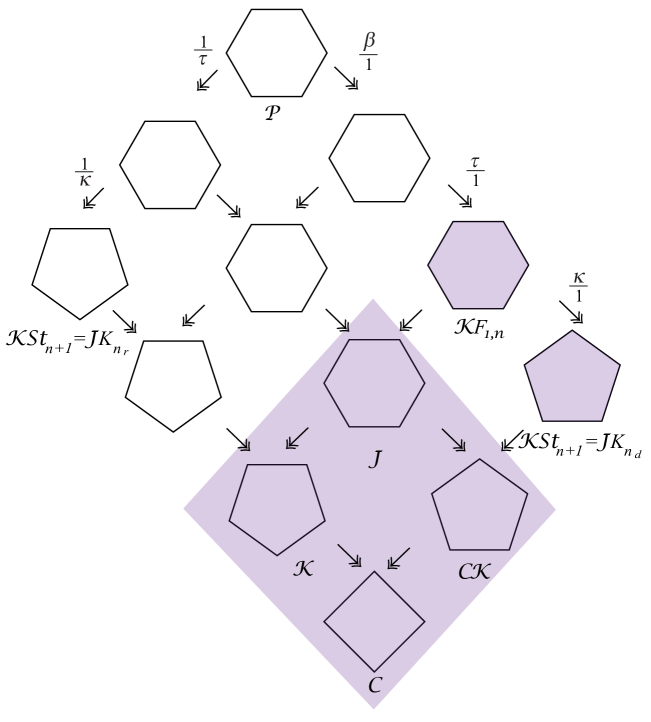
Figure 6. These are the 2-dimensional terms in the same sequences as in Example 4.3.

In this section four more sequences of our sets of painted trees, with their relations, will be shown to be isomorphic as posets to face lattices of convex polytopes. Two of these are the species whose structure types are: a forest of corollas grafted to a weakly ordered tree (stellohedra) or a weakly ordered forest grafted to a corolla (stellohedra again). A third is the species whose structure type is the weakly ordered forest grafted to a weakly ordered tree (permutohedra). Finally the species whose structure type is a forest of plane rooted trees grafted to a weakly ordered tree (pterahedra). There remain four cases in Example 4.3 that we leave as a conjecture. (These latter four are the ones which do not have a label naming them under their picture).

Some of our proofs and corollaries will use the concept of tubings, which we review next.

4.3. Tubes, tubings and marked tubings.

The definitions and examples in this section are largely taken from [17] and [10]. They are based on the original definitions in [7], with only the slight change of allowing a universal tube, as in [9].

Definition 4.5.

Let $G$ be a finite connected simple graph. A tube is a set of nodes of $G$ whose induced graph is a connected subgraph of $G$. For a given tube $t$ and a graph $G$, let $G(t)$ denote the induced subgraph on the graph $G$. We will often refer to the induced graph itself as the tube. Two tubes $u$ and $v$ may interact on the graph as follows:

1. Tubes are nested if $u\subset v$.

2. Tubes are far apart if $u\cup v$ is not a tube in $G,$ that is, the induced subgraph of the union is not connected, (equivalently none of the nodes of $u$ are adjacent to a node of $v$).

Tubes are compatible if they are either nested or far apart. We call $G$ itself the universal tube. A tubing $U$ of $G$ is a set of tubes of $G$ such that every pair of tubes in $U$ is compatible; moreover, we force every tubing of $G$ to contain (by default) its universal tube. By the term $k$-tubing we refer to a tubing made up of $k$ tubes, for $k\in\{1,\dots,n\}.$

Remark 4.6.

For connected graphs our definition here is equivalent to that in [24]. In [7] and [10] the universal tube is not considered a tube, nor included in tubings. This however leads to a poset of tubings which is isomorphic to the one in this paper.

When $G$ is a disconnected graph with connected components $G_{1}$, …, $G_{k}$, there are alternate definitions in the literature. In [25] and [24], as well as in [3], the connected components are all tubes and must all be included in every tubing. We will refer to this as a building set tubing since it contains all maximal elements.

Alternatively, in [7], [9] and [16], as well as in [15], the additional condition for disconnected graphs is as follows: If $u_{i}$ is the tube of $G$ whose induced graph is $G_{i}$, then no tubing of $G$ contains all of the tubes $\{u_{1},\ldots,u_{k}\}$. However, the universal tube is still included in all tubings despite being itself disconnected.

Parts (a)-(c) of Figure 8 from [9] show examples of allowable tubings, whereas (d)-(f) depict the forbidden ones.

Figure 8. (a)-(c) Allowable tubings and (d)-(f) forbidden tubings, figure from [9].

Let ${\mbox{Tub}(G)}$ denote the set of tubings on a graph $G.$ As shown in [7, Section 3], for a graph $G$ with $n$ nodes, the graph associahedron ${\mathcal{K}}G$ is a simple, convex polytope of dimension $n-1$ whose face poset is isomorphic to ${\mbox{Tub}(G)}$, partially ordered by the relationship $U\prec U^{\prime}$ if $U^{\prime}\subseteq U.$

The vertices of the graph associahedron are the $n$-tubings of $G.$ Faces of dimension $k$ are indexed by $(n-k)$-tubings of $G.$ In fact, the barycentric subdivision of ${\mathcal{K}}G$ is precisely the geometric realization of the described poset of tubings.

To describe the face structure of the graph associahedra we need a definition from [7, Section 2].

Definition 4.7.

For graph $G$ and a collection of nodes $t$, construct a new graph $G^{*}(t)$ called the reconnected complement: If $V$ is the set of nodes of $G$, then $V-t$ is the set of nodes of $G^{*}(t)$. There is an edge between nodes $a$ and $b$ in $G^{*}(t)$ if $\{a,b\}\cup t^{\prime}$ is connected in $G$ for some $t^{\prime}\subseteq t$.

Figure 9 illustrates some examples of graphs along with their reconnected complements.

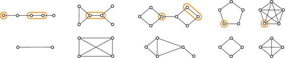
Figure 9. Examples of tubes and their reconnected complements. Figure from [17].

Theorem 4.8.

[7, Theorem 2.9] Let $V$ be a facet of ${\mathcal{K}}G,$ that is, a face of dimension $n-2$ of ${\mathcal{K}}G$, where $G$ has $n$ nodes. $V$ corresponds to $t$, a single, non-universal, tube of $G$ . The face poset of $V$ is isomorphic to ${\mathcal{K}}G(t)\times\mathcal{K}G^{*}(t)$.

We will consider a related operation on graphs. The suspension of $G$ is the graph ${\mathfrak{S}}G$ whose set of nodes is obtained by adding a node $0$ to the set ${\mbox{Nod}(G)}$, of nodes of $G$, and whose edges are defined as all the edges of $G$ together with the edges $\{0,v\}$ for ${v\in\mbox{Nod}(G)}.$

The reconnected complement of $\{0\}$ in ${\mathfrak{S}}G$ is the complete graph ${\mathcal{K}}_{n}$ for any graph $G$ with $n$ nodes. Note that the star graph $St_{n}$ is the suspension of the graph which has $n$ nodes and no edge, while the fan graph $F_{1,n}$ is the suspension of the path graph on $n$ nodes. The suspension of a complete graph $K_{n}$ is the complete graph $K_{n+1}.$

It turns out that this construction of the graph multiplihedra is a special case of a more general construction on certain polytopes called the generalized permutahedra as defined by Postnikov in [25]. The lifting of a generalized permutahedron, and a nestohedron in particular, is a way to get a new generalized permutahedron of one greater dimension from a given example, using a factor of $q\in[0,1]$ to produce new vertices from some of the old ones [3]. This procedure was first seen in the proof that Stasheff’s multiplihedra complexes are actually realized as convex polytopes [13].

Soon afterwards the lifting procedure was applied to the graph associahedra–well-known examples of nestohedra first described by Carr and Devadoss. We completed an initial study of the resulting polytopes, dubbed graph multiplihedra, published as [9].

This application raised the question of a general definition of lifting using $q.$ At the time it was also unknown whether the results of lifting, then just the multiplihedra and the graph-multiplihedra, were themselves generalized permutahedra. These questions were both answered in the recent paper of Ardila and Doker [3]. They defined nestomultiplihedra and showed that they were generalized permutohedra of one dimension higher in each case.

We refer the reader to Ardila and Doker [3] for the general definitions. Here we need only the following definitions, from [9]. Combinatorially, lifting of a graph associahedron occurs when the notion of a tube is extended to include markings.

Definition 4.9.

A marked tube of a graph $G$ is a tube with one of three possible markings:

1. a thin tube    given by a solid line,

2. a thick tube    given by a double line, and

3. a broken tube    given by fragmented pieces.

Marked tubes $u$ and $v$ are compatible if

1. they form a tubing and

2. if $u\subset v$ where $v$ is not thick, then $u$ must be thin.

A marked tubing of $G$ is a tubing of pairwise compatible marked tubes of $G$.

A partial order is now given on marked tubings of a graph $G$. This poset structure is then used to construct the graph multiplihedron below.

Definition 4.10.

The collection of marked tubings on a graph $G$ can be given the structure of a poset. For two marked tubings $U$ and $U^{\prime}$ we have $U\prec U^{\prime}$ if $U$ is obtained from $U^{\prime}$ by a combination of the following four moves. Figure 10 provides the appropriate illustrations, with the top row depicting $U^{\prime}$ and the bottom row $U$.

1. Resolving markings: A broken tube becomes either a thin tube (10a) or a thick tube (10b).

2. Adding thin tubes: A thin tube is added inside either a thin tube (10c) or broken tube (10d).

3. Adding thick tubes: A thick tube is added inside a thick tube (10e).

4. Adding broken tubes: A collection of compatible broken tubes $\{u_{1},\ldots,u_{n}\}$ is added simultaneously inside a broken tube $v$ only when $u_{i}\Subset v$ and $v$ becomes a thick tube; two examples are given in (10f) and (10g).

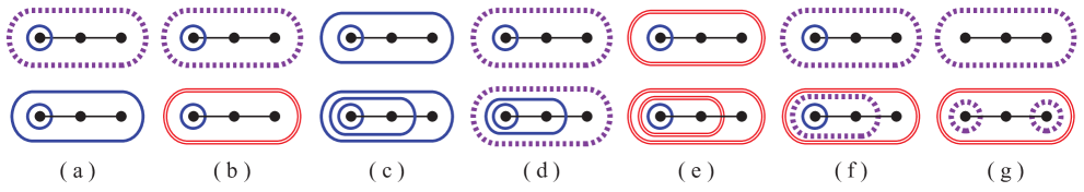
Figure 10. The top row are the tubings and bottom row their refinements. Figure based on original in [9].

Here is the key idea from [9]: for a graph $G$ with $n$ nodes, the graph multiplihedron ${\mathcal{J}}G$ is a convex polytope of dimension $n$ whose face poset is isomorphic to the set of marked tubings of $G$ with the poset structure given above.

There are two important quotient polytopes mentioned in [9]: ${\mathcal{J}}G_{d}$ and ${\mathcal{J}}G_{r}$ for a given graph $G.$ The former is called the graph composihedron. Its faces correspond to marked tubings, but for which no thin tubes are allowed to be inside another thin tube. In terms of equivalence of tubings, the face poset of ${\mathcal{J}}G_{d}$ is isomorphic to the poset ${\mathcal{J}}G$ modulo the equivalence relation on marked tubings generated by identifying any two tubings $U\sim V$ such that $U\prec V$ in ${\mathcal{J}}G$ precisely by the addition of a thin tube inside another thin tube, as in Figure 10(c). Thus an equivalence class of tubings can be represented by its maximum member: a tubing with no thin tubes inside any other thin tube. The graph composihedron is defined via geometric realization in [9]. The relations in Figure 10 still hold, but some of them appear differently, and one (c) is no longer present in Figure 11.

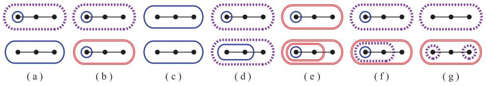
Figure 11. The top row are the tubings and bottom row their refinements, in the graph composihedron. These are altered versions (shown up to equivalence) of the relations in Figure 10. In fact (c) is the reflective relation.

The polytope ${\mathcal{J}}G_{r}$ has faces which correspond to marked tubings, but for which no thick tubes are allowed to be inside another thick tube. In terms of equivalence of tubings, the face poset of ${\mathcal{J}}G_{r}$ is isomorphic to the poset ${\mathcal{J}}G$ modulo the equivalence relation on marked tubings generated by identifying any two tubings $U\sim V$ such that $U\prec V$ in ${\mathcal{J}}G$ precisely by the addition of a thick tube, as in Figure 10(e).Thus an equivalence class of tubings can be represented by its maximum member: a tubing with no thin tubes inside any other thin tube. ${\mathcal{J}}G_{r}$ is defined via geometric realization in [9]. For connected graphs $G$, the polytope ${\mathcal{J}}G_{r}$ is combinatorially equivalent to the graph cubeahedron $\mathbb{C}G,$ as defined in [11].

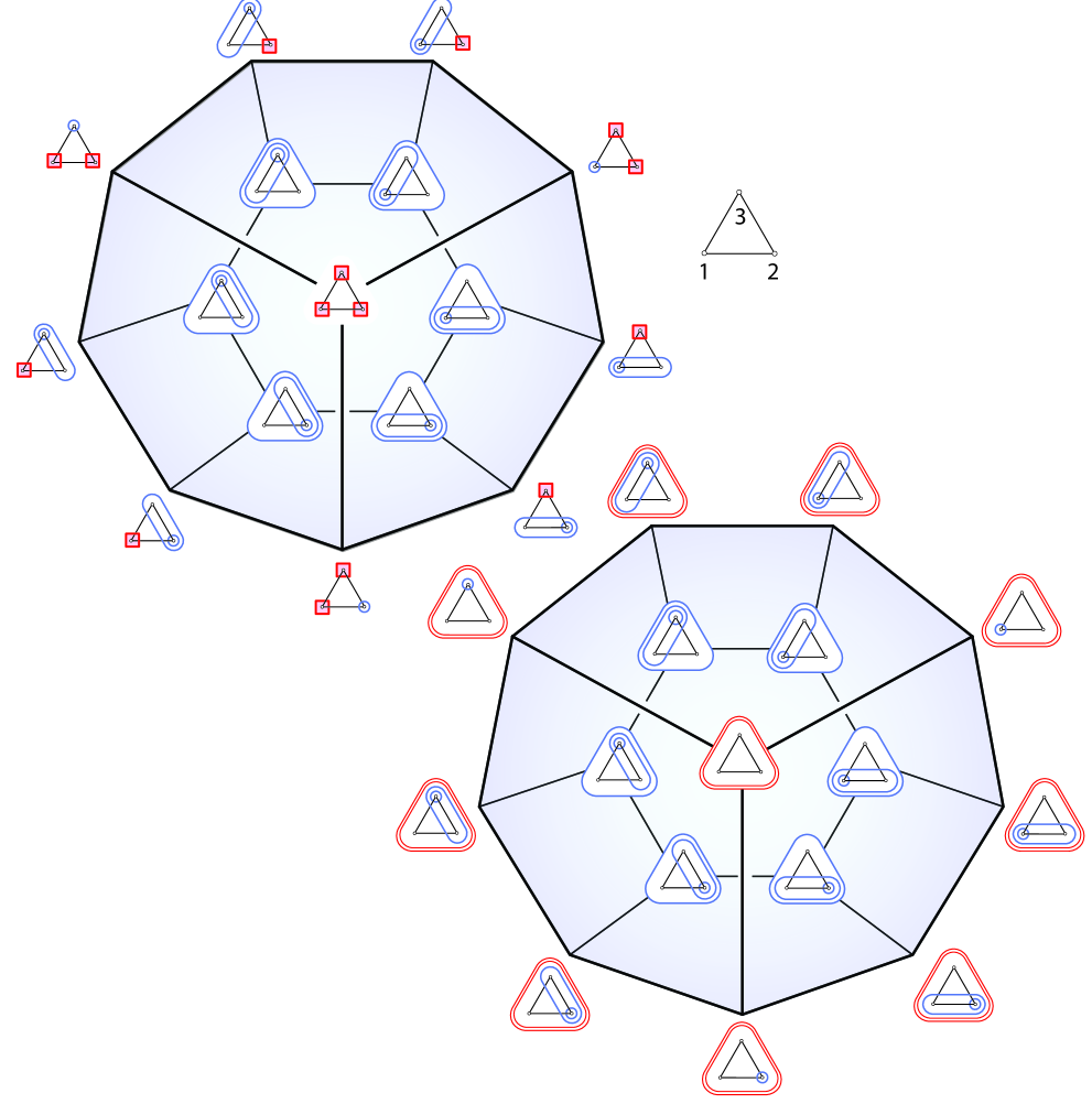
Figure 21. Another stellahedra bijection: the complete graph cubeahedron indexed by design tubings.

The graph cubeahedron $\mathbb{C}K_{n}$ is described in [11] as comprising the design-tubings on the complete graph. In Figure 21 we show the correspondence between labels of vertices: range-equivalence classes of marked tubings and design tubings. The isomorphism claimed in [11] is easily described: design tubes (square tubes) correspond to the nodes not inside any thin or broken tube; while round tubes in the design tubing correspond to thin tubes. Broken tubes contain any nodes not in any tube of the design tubing.

For this reason we refer to the entire class of polytopes ${\mathcal{J}}G_{r}$ as the (general) graph cubeahedra. In fact the description of $\mathbb{C}G$ using design tubings which is given in [11] is not difficult to extend to graphs with multiple components: we only need to introduce the universal (round) tube. For example, the graph cubeahedron for the edgeless graph is the hypercube with a single truncated vertex.

The four well-known examples of polytopes from Example 4.3 can be seen as tubing posets, as pointed out in [9]. The multiplihedra $\mathcal{J}=\mathcal{J}P$ have face posets equivalent to the marked tubes on path graphs $P$. The composihedra are the domain quotients of these: $\mathcal{J}P_{d}$; and the associahedra are the range quotients of these: $\mathcal{J}P_{r}.$ The cubes show up as the result of taking both quotients simultaneously.

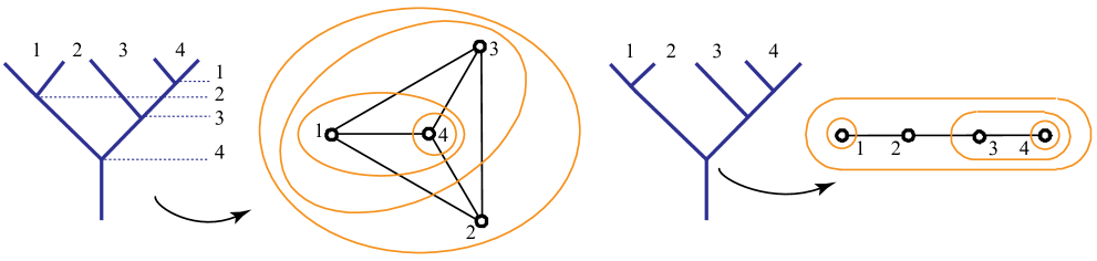
Figure 12. The permutation $\sigma=(2431)\in S_{4}$ pictured as an ordered tree and as a tubing of the complete graph; An unordered binary tree, and its corresponding tubing. Figure from [17].

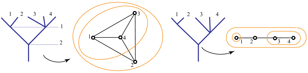
Figure 13. The ordered partition $(\{1,2,4\},\{3\})$ pictured as a leveled tree and as a tubing of the complete graph; the underlying tree, and its corresponding tubing. Figure from [17].

4.4. Permutohedra

First we prove that the poset of painted trees made by grafting a weakly ordered forest to a weakly ordered base tree is the face poset of a polytope. It turns out that for painted trees with $n$ leaves this polytope is the permutohedron $\mathcal{P}_{n}.$ It is well known (see [18]) that the permutohedron has faces indexed by the weak orders, which in turn may be represented by weakly ordered trees. The face poset is the partial ordering of these trees by refinements.

Theorem 4.11.

There is an isomorphism $\varphi$ from the poset of $(n+1)$-leaved weakly ordered trees to the painted growth preorder of $n$-leaved weakly ordered forests grafted to weakly ordered trees.

Proof.

The isomorphism and its inverse are described as switching between the paint line and an extra branch. Given a weakly ordered tree $t$, we find $\varphi(t)$ by adding a paint line at the level of left-most node of $t$, and then deleting the left-most branch of $t$. Finally the remaining nodes are ordered, above and below the paint line, according to their original vertical order in $t.$ The inverse is straightforward. Here is a picture of the process:

Next we argue that the isomorphism just described respects the poset structures. If $a\prec b$ for two weakly ordered trees, we have that the weak ordering of the nodes of $a$ is a refinement of the weak ordering for $b.$ We can visualize this refinement as the growing of some internal edges of $a$ to break ties between nodes that were at the same level. If the refinement involves breaking a tie that does not include the left-most node (see level 2 in the above picture), then the same growing produces the same relation between the painted tree images $\varphi(a)$ and $\varphi(b).$ If the growing does break a tie involving the left-most node (see level 4 in the above picture), then the image of $b$ may differ from that of $a$ only in that the set of nodes of $\varphi(a)$ which coincide with the paint line will be a subset of those in $\varphi(b)$. This can be seen as growing edges at some half-painted nodes. Here is an example of the latter case, with trees related to those in the above pictured example:

∎

This theorem immediately implies that the poset of $n$-leaved weakly ordered forests grafted to weakly ordered trees is isomorphic to the face poset of the $n$-dimensional permutohedron. That is because the poset of $(n+1)$-leaved weakly ordered trees is well known to represent the face poset of the permutohedron (via seeing each tree as a weak order of $[n]$, that is, an ordered partition.)

A corollary, from [9], is that the poset of $n$-leaved weakly ordered forests grafted to weakly ordered trees is isomorphic to the face poset of the $n$-dimensional graph multiplihedron of the complete graph.

4.5. Stellohedra

Now we prove that the poset of painted trees made by grafting a forest of corollas to a weakly ordered base tree is the face poset of a polytope. It turns out that for painted trees with $n+1$ leaves this polytope is the graph-associahedron ${\mathcal{K}}G$ where $G$ is the star graph $St_{n}.$

Recall that the star graph $St_{n}$ is defined as follows: we use the set $\{0,1,2,\dots,n\}$ as the set of nodes. Edges are $\{0,i\}$ for $i=1,\dots,n.$

Theorem 4.12.

The poset of tubings on the star graph $St_{n}$ is isomorphic to the poset of $n$-leaved forests of corollas grafted to weakly ordered trees.

Proof.

We first note that any tubing $T$ of the star graph includes a unique smallest tube $t_{0}$ which contains node 0. All other tubes of $T$ are either contained in $t_{0}$ or contain $t_{0},$ since the node 0 is adjacent to all other nodes. The tubes contained in $t_{0}$ form a tubing of an edgeless graph. The tubes containing $t_{0}$ form a tubing on the reconnected complement of $t_{0}$, which is the complete graph on the nodes not in $t_{0}.$ Here the key idea is that the tube $t_{0}$ is analogous to the half-painted nodes. See Figure 14.

Now we use two facts shown in [7]: that the permutohedron is combinatorially equivalent to the graph-associahedron of the complete graph, and that the simplex is combinatorially equivalent to the graph-associahedron of the edgeless graph, which in turn is equivalent to the Boolean lattice of subsets of its nodes. Recall that the permutohedron is also indexed by the weakly ordered trees, leading to an isomorphism between tubings and trees as seen in Figures 12 and 13.

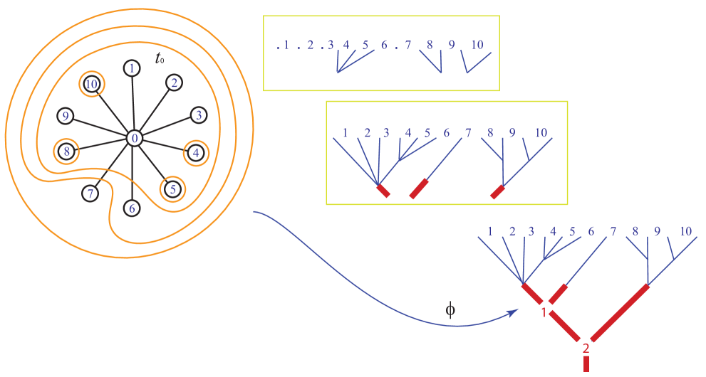
Figure 14. A tubing $T$ on the star graph and its bijective image in the corollas over weakly ordered trees. The three steps are shown for constructing $\phi(T).$

Thus the bijection $\phi$ we want takes a tubing $T$ on the star graph $S=S_{n}$ to a painted tree. This bijection is constructed from the bijection $\alpha$ from tubings on an edgeless graph to subsets of $n$ gaps between leaves (corresponding to nodes in a unpainted forest of corollas); together with the bijection $\beta$ from tubings on a complete graph with $j$ vertices to weakly ordered trees with $j+1$ leaves.

The construction of $\phi$ proceeds as follows. First the nodes $1,\dots,n$ of the star graph correspond to the gaps (between leaves) $1,\dots,n$ of the output tree. The tubing of the subgraph inside of $t_{0}$ maps via $\alpha$ to a subset of $[n],$ and that subset is precisely the subset of the gaps which correspond to unpainted nodes (of corollas) in our output tree. Second, nodes that are inside $t_{0}$ but not inside any smaller tube determine the gaps that coincide with the paint line, half-painted nodes on our output tree. Finally the tubing outside of $t_{0}$ maps via $\beta$ to the painted weakly ordered tree. The inverse of $\phi$ is the straightforward reversal of these steps. An example is seen in Figure 14.

Checking that this bijection preserves the ordering is straightforward. Covering relations in the stellohedron are face inclusions, which each correspond to adding one tube to a tubing. The addition of a singleton tube inside of $t_{0}$ corresponds under our bijection to growing an unpainted edge at a half-painted node (and then applying $\kappa.$)

The addition of a tube just inside of $t_{0}$ that contains all the singleton tubes, so in effect creating a new $t_{0}$, corresponds to growing some painted edges from half-painted nodes.

The addition of a tube outside of $t_{0}$ corresponds to growing a painted edge at a painted node. The three possibilities are illustrated here: the first has a singleton tube added (around vertex 9) compared with the original tubing in Figure 14.

∎

The isomorphism of vertices of the polytopes in 3 dimensions is shown pictorially in Figure 15.

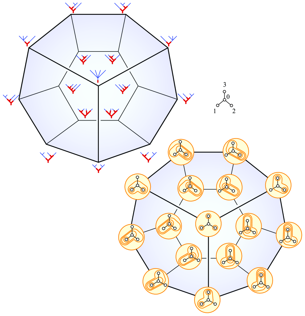
Figure 15. Two pictures of the stellohedron, via the bijection in Theorem 4.12.

Next we show that the stellohedra can also be seen as the domain and range quotients ${\mathcal{J}}G_{d}$ and ${\mathcal{J}}G_{r}$ of the multiplihedron ${\mathcal{J}}G$ where $G$ is the complete graph.

Theorem 4.13.

The graph-composihedron for a complete graph $\mathcal{K}_{n}$ is combinatorially equivalent to the stellohedron for the star-graph $St_{n+1}.$

Proof.

We can most easily see the isomorphism by using the stellohedra just found in Theorem 4.12, that is, by showing an isomorphism to painted trees.

We show a bijection $\phi^{\prime}$ from the graph-composihedron of the complete graph to the set $\widetilde{C/D}$ of forests of corollas grafted to weakly ordered trees. The nodes $1,\dots,n$ of the complete graph correspond to the gaps (between leaves) $1,\dots,n$ of the tree. Here the key idea is that now a broken tube $t_{0}$ plays the same role as the half-painted nodes in the corresponding tree, and a single thin tube the role of the unpainted nodes. The steps in the construction of the bijection $\phi^{\prime}$ are analogous to those in the proof of Theorem 4.12, as follows:

The bijection $\phi^{\prime}$ takes as input a marked tubing on the complete graph with no thin tubes inside another thin tube. It outputs a painted tree as follows: if there is a single thin tube $t=\{v_{1},v_{2},\dots,v_{k}\}$ then the like-numbered gaps of the output will correspond to nodes of unpainted corollas. Nodes that are inside a broken tube but not inside any thin tube of the input correspond to the gaps of the output that correspond to half-painted nodes. Any nodes outside of all the thin or broken tubes in the input correspond to nodes of the weakly ordered base tree in the output, and this mapping is via the previously mentioned bijection between weak orders and tubings on the complete graph. Note that the reconnected complement of the largest thin or broken tube is a complete graph. The inverse of $\phi^{\prime}$ is the straigtforward reversal of these steps. An example of the bijection $\phi^{\prime}$ is seen in Figure 16.

We check that this bijection $\phi^{\prime}$ preserves the ordering. Note that the relations are simpler than in general for marked tubes since the tubings must all be completely nested, and since thin tubes inside of thin tubes are ignored (via the equivalence). Thus the relations in the Figure 11(c) and 11(g) need not be checked. The relations in Figure 11(a) and (d) correspond to growing unpainted edges from half-painted nodes. The relations in Figure 11(b) and (f) correspond to growing painted edges from half-painted nodes. The relation in Figure 11(e) corresponds to growing a painted edge from a painted node. Examples of the preservation of ordering via $\phi^{\prime}$ re seen in Figure 17. 3-dimensional examples are seen in Figure 19. See Figure 22 for some isomorphic chains. ∎

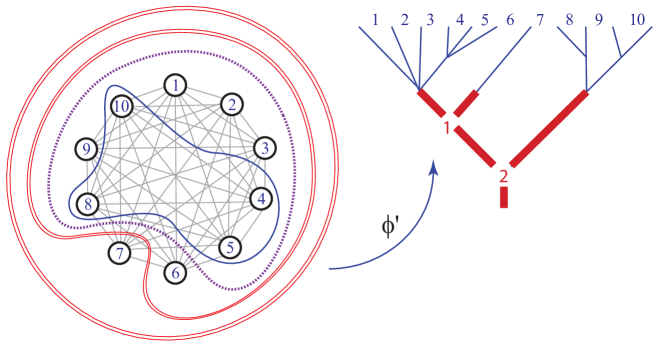
Figure 16. A marked tubing on the complete graph, representing an element of the complete-graph-composihedron (no structure is shown inside the thin tube) and its bijective image in the forest of corollas over a weakly ordered tree.

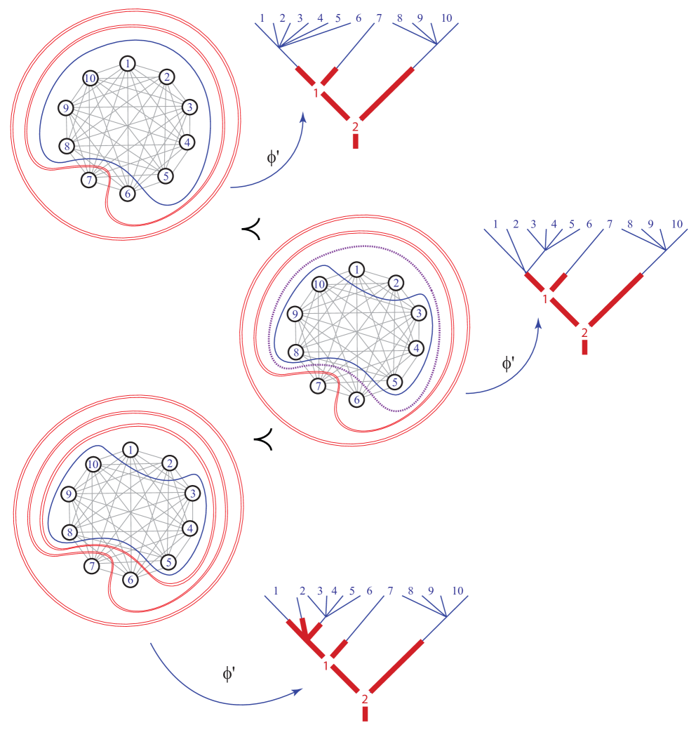
Figure 17. The first (upper) example of $\phi^{\prime}$ has source and target related to Figure 16 by a adding a tube as in Figure 11(d) and growing an unpainted edge from a half-painted node, and then forgetting structure in both pictures. The other two relations are from Figure 11(a) and (b) (right to left).

Moreover, we will show that the poset of painted trees made by grafting a weakly ordered forest to a base corolla is the face poset of a polytope. It turns out that for painted trees with $n+1$ leaves this polytope is again the graph-associahedron ${\mathcal{K}}G$ where $G$ is the star graph $St_{n}.$

First, however, we show a bijection from the range-quotients of the complete graph multiplihedron (the complete graph-cubeahedron) to the weakly ordered forests grafted to corollas.

Theorem 4.14.

The poset of $n+1$-leaved weakly ordered forests grafted to corollas is combinatorially equivalent to the graph-cubeahedron for a complete graph $\mathcal{K}_{n}.$

Proof.

This proof follows the pattern of the previous one, so we leave most of it to the reader. Note that any nodes outside of the broken $t_{0}$ tube in the input correspond to the painted corolla base tree of the ouput. The tubing inside a largest thin tube (which contains a clique) in the input corresponds to the gaps (between leaves) that end in nodes of the unpainted weakly ordered forest of the output. Nodes that are inside a broken tube but not inside any thin tube determine the gaps that coincide with the paint line. An example of the bijection is seen in Figure 18.

The fact that this bijection preserves the ordering is seen just as in the proof of Theorem 4.13. 3-dimensional examples are seen in Figure 20. See Figure 22 for some isomorphic chains. ∎

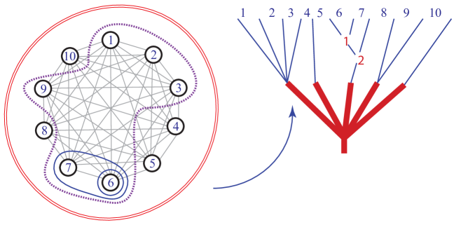
Figure 18. A marked tubing on the complete graph, representing an element of the complete-graph-cubahedron (no structure is shown outside the broken tube) and its bijective image in the weakly ordered forests over corollas.

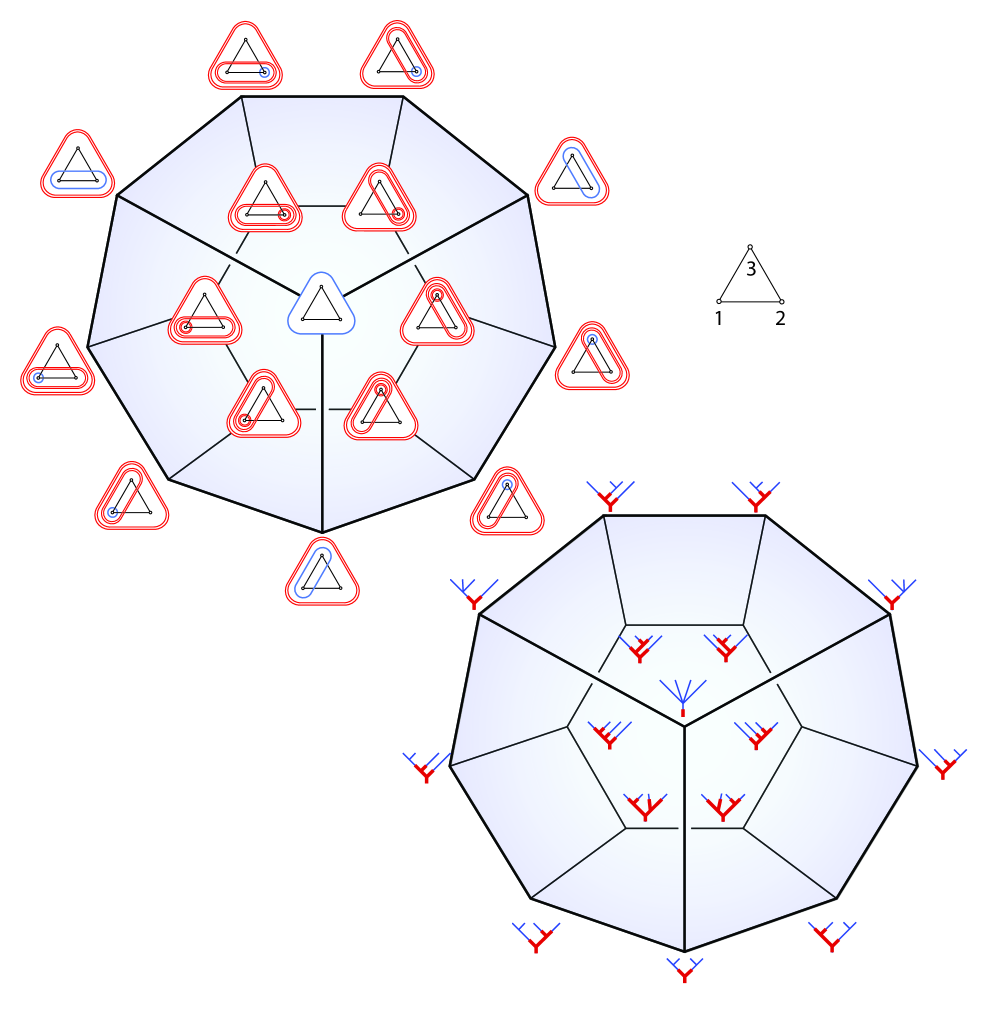
Figure 19. Another stellahedra bijection via Theorem 4.13: when $K_{n}$ is the complete graph then $\mathcal{J}K_{n_{d}}$ (the complete graph composihedron) is the stellohedron.

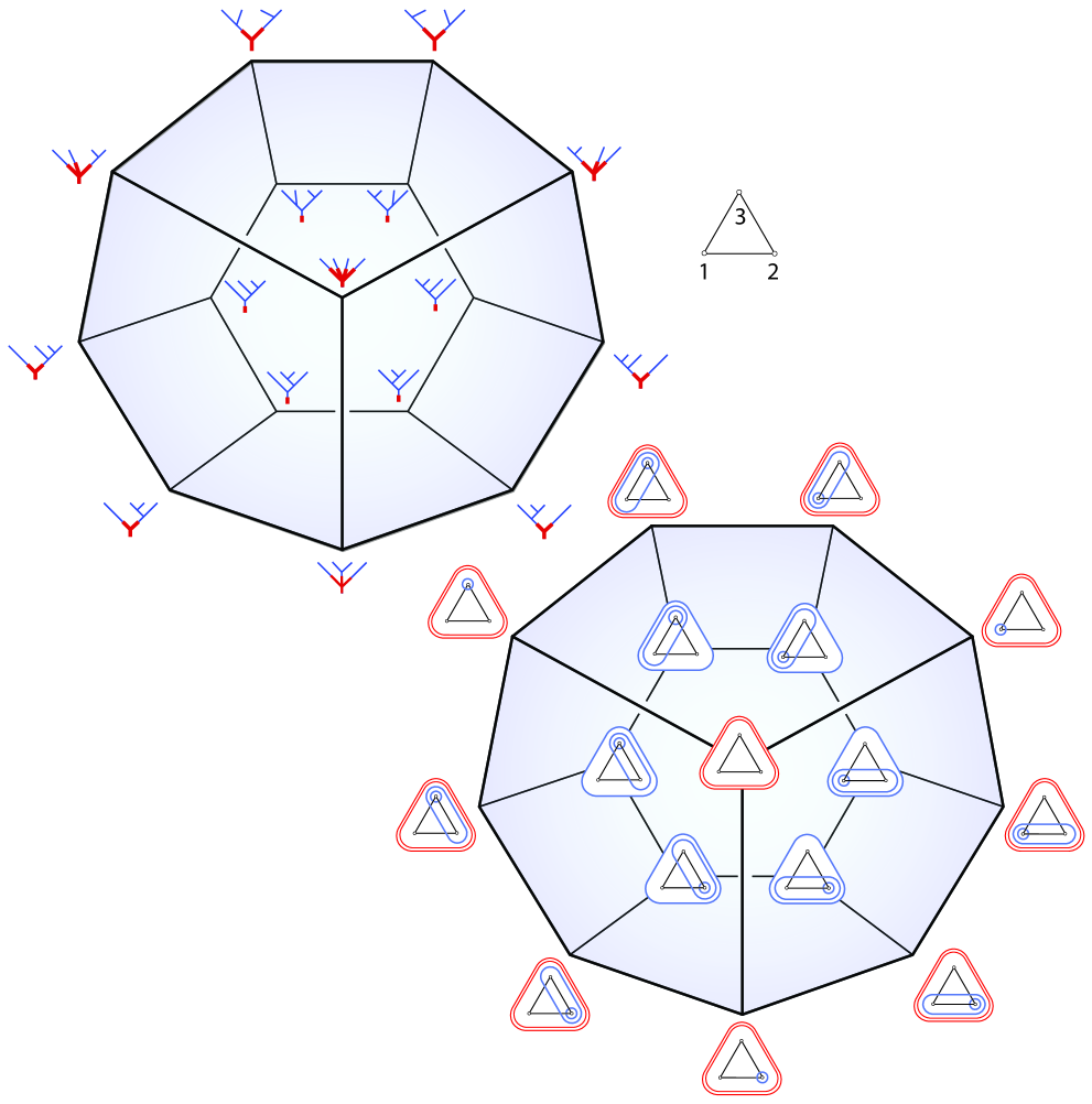
Figure 20. Another stellahedra bijection via Theorem 4.15: the composition of ordered forests with corollas, seen in bijection with the complete graph cubeahedron.

We now can finish with the following:

Theorem 4.15.

The weakly ordered forests grafted to corollas are isomorphic to the stellohedra.

Proof.

By Theorem 62 of [22], the graph-cubeahedron for a complete graph $\mathcal{K}_{n}$ is combinatorially equivalent to the stellohedron for the star-graph $St_{n+1}.$ Here is a brief description of the poset isomorphism described in that paper: if the star graph $St_{n+1}$ has node 0 as its center, and the nodes of the complete graph are $1,\dots,n$, then a square tube on the complete graph is mapped to itself, as a round tube; and round tubes on the complete graph are mapped to their complement plus the node 0 on the star graph. We demonstrate this isomorphism in Figure 22. Thus the theorem is shown, by composition with the isomorphism in our Theorem 4.14. ∎

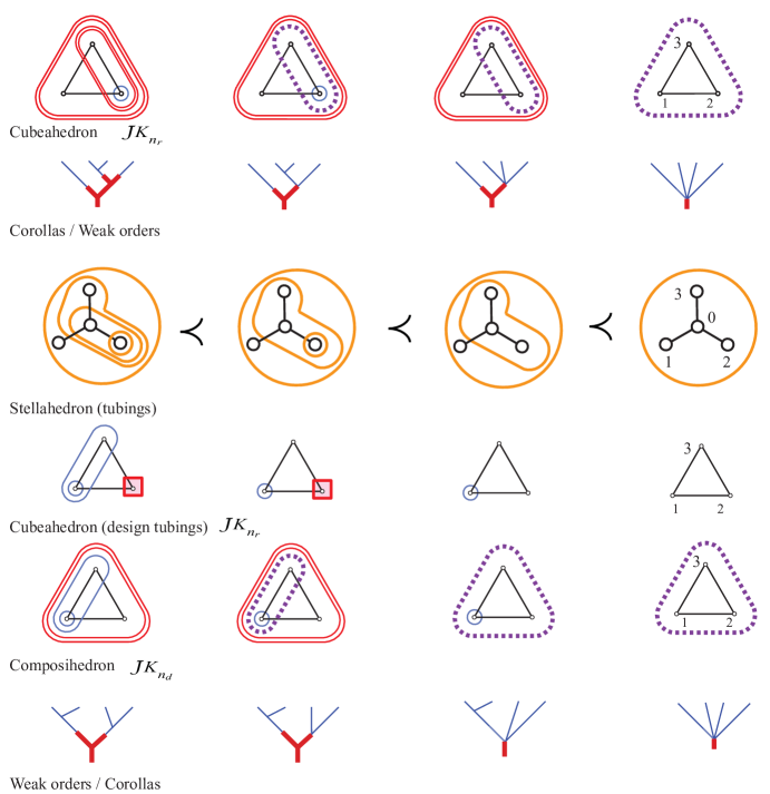
Figure 22. Here we bring together six isomorphic flags from the 3-dimensional stellohedra shown above.

4.6. Pterahedra

The aim of this subsection is to prove that the poset of painted trees made by grafting a forest of plane rooted trees to a weakly ordered base tree is the face poset of a polytope. It turns out that for painted trees with $n+1$ leaves this polytope is the graph-associahedron $\mathcal{K}F_{1,n}$ where the fan graph $F_{1,n}$ is the suspension of the path graph $P_{n}$.

More precisely, the fan graph $F_{1,n}$ is defined as follows: the set of nodes of $F_{1,n}$ is $[n]_{0}$, while an edge of the graph is given either by the pair $\{i,i+1\}$, for some $i=1,\dots,n-1$, or by a pair $\{0,i\}$, for some $i=1,\dots,n$.

Theorem 4.16.

The poset of tubings on the fan graph $F_{1,n}$ is isomorphic to the poset of $n$-leaved forests of plane trees grafted to weakly ordered trees.

Proof.

Recall that any tubing $T$ of the fan graph includes a unique smallest tube $t_{0}$ which contains the node $0$. As the node $0$ is adjacent to all other nodes, the other tubes of $T$ are either contained in $t_{0}$ or contain $t_{0}$. The tubes contained in $t_{0}$ form a tubing of a graph which is a (possibly) disconnected set of line graphs. The tubes containing $t_{0}$ form a tubing on the reconnected complement of $t_{0}$, which is the complete graph on the nodes which do not belong to $t_{0}$.

There exists a canonical bijection between the poset of weakly ordered trees with $n+1$ leaves and the poset ${\mbox{Tub}(K_{n})}$ of tubings on the complete graph: pictured in Figures 12 and 13. The restriction of this map to the set of plane trees, gives a bijection between this poset and the poset ${\mbox{Tub}(P_{n})}$ of tubings on the path graph.

Thus the bijection from the poset ${\mbox{Tub}(F_{1,n})}$ of tubings on the fan graph to our set of painted trees is obtained from the bijection between ${\mbox{Tub}(K_{m})}$ and the set of weakly ordered trees, together with the bijections between the set ${\mbox{Tub}(P_{m})}$ of tubings on the path graph and the set of plane rooted trees with $m+1$ leaves, for $m\geq 1$. The tube $t_{0}$ plays the same role as the paint line in the corresponding tree. The nodes $1,\dots,n$ of the fan graph $F_{1,n}$ correspond to the gaps (between leaves) $1,\dots,n$ of the plane rooted tree. For any tubing $T\in{\mbox{Tub}(F_{1,n})}$ tubing outside of $t_{0}$ maps to the painted weakly ordered tree, the tubings inside $t_{0}$ map to the unpainted trees, and nodes that are inside $t_{0}$ but not inside any smaller tube determine the gaps that coincide with the paint line. Examples are seen in Figure 23.

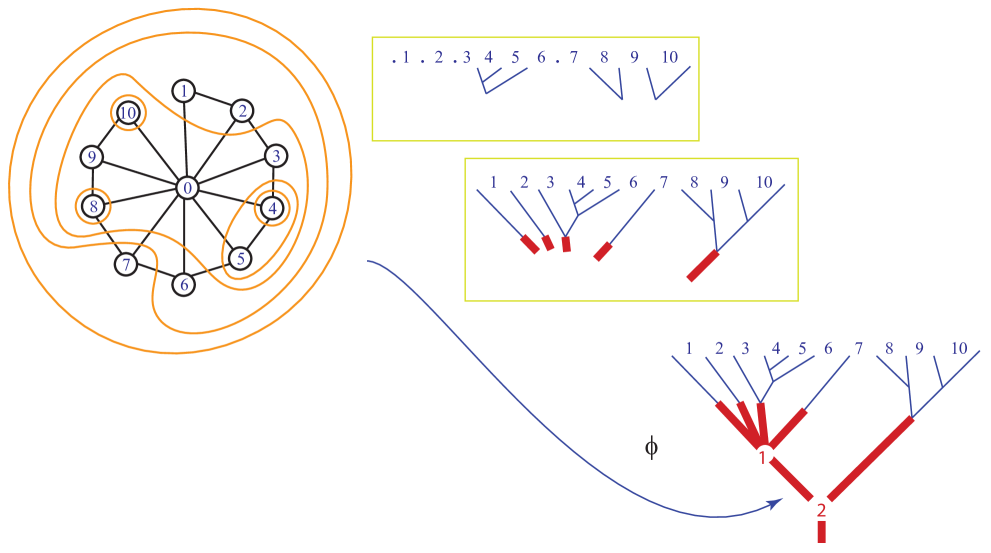
Figure 23. Example of the bijection in Theorem 4.16. The steps are shown left to right.

The fact that this bijection preserves the ordering follows easily from the definitions. Just note that adding a tube to a tubing of the fan graph corresponds to growing an internal edge in the tree. Adding a tube far outside of $t_{0}$ corresponds to growing an edge in the painted base. Adding a tube containing node 0 just inside $t_{0}$ (so that it becomes the new $t_{0}$) corresponds to growing painted edge(s) from a half-painted node. Adding a tube just inside $t_{0}$ that does not contain node 0 corresponds to growing unpainted edge(s) from a half-painted node. Adding a tube further inside of $t_{0}$ (that does not contain node 0) corresponds to growing an edge in the unpainted forest. ∎

The isomorphism in 3 dimensions is shown pictorially in Figure 24.

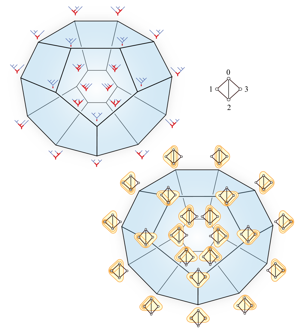
Figure 24. Two pictures of the pterahedron, via the bijection from Theorem 4.16.

4.7. Enumeration

As well as uncovering the equivalence between the pterahedra and the fan-graph associahedra, we found some new counting formulas for the vertices and facets of the pterahedra.

First the vertices of the pterahedra, which are forests of binary trees grafted to an ordered tree. If there are $k$ nodes in the ordered, painted portion of a tree, then there are:

• $k!$ ways to make the ordered portion of this tree with $k$ nodes,

• $k+1$ leaves of the ordered portion of this tree, and

• $n-k$ remaining nodes to be distributed among the $k+1$ binary trees that will go on the leveled/painted leaves.

Thus the number of vertices of the pterahedron, labeled by trees with $n$ nodes, is:

$v(n)=\sum\limits_{k=0}^{n}[~{}k!\sum\limits_{\begin{subarray}{c}\gamma_{0}+\dots+\gamma_{k}\\ =n-k\end{subarray}}~{}(\prod\limits_{i=0}^{k}C_{\gamma_{i}})~{}]$.

where $C_{j}$ is the $j$th Catalan number. As an example, the number of trees with $n=4$ is:

$$0!~{}[C_{4}]$$

$$+1!~{}[C_{3}C_{0}+C_{2}C_{1}+C_{1}C_{2}+C_{0}C_{3}]$$

$$+2!~{}[C_{2}C_{0}C_{0}+C_{1}C_{1}C_{0}+C_{1}C_{0}C_{1}+C_{0}C_{2}C_{0}+C_{0}C_{1}C_{1}+C_{0}C_{0}C_{2}]$$

$$+3!~{}[C_{1}C_{0}C_{0}C_{0}+C_{0}C_{1}C_{0}C_{0}+C_{0}C_{0}C_{1}C_{0}+C_{0}C_{0}C_{0}C_{1}]$$

$$+4!~{}[C_{0}C_{0}C_{0}C_{0}C_{0}]$$

$$=1(14)+1(14)+2(9)+6(4)+24(1)$$

$$=14+14+18+24+24$$

$$=94$$

We have computed the cardinalities for $n=0$ to 9 and they are shown in Table 3.

Table 3. The number $v(n)$ vertices of the pterahedra, $n=0$ to 9

$n$	$v(n)$	$n$	$v(n)$
0	1	5	464
1	2	6	2652
2	6	7	17,562
3	22	8	133,934
4	94	9	1,162,504

There does not seem to be an entry for this sequence in the OEIS.

Examination of the computations of $v(n)$ leads to an interesting discovery. If we strip off the factorial factors in $v(n)$ and build a triangle of just the sums of $C_{\gamma_{i}}$ products, it appears we are building the Catalan triangle.

1
1	1
2	2	1
5	5	3	1
14	14	9	4	1
42	42	28	14	5	1
132	132	90	48	20	6	1
429	429	297	165	75	27	7	1
1430	1430	1001	572	275	110	35	8	1
4862	4862	3432	2002	1001	429	154	44	9	1

For example,

$v(4)=94=0!(\textbf{14})+1!(\textbf{14})+2!(\textbf{9})+3!(\textbf{4})+4!(\textbf{1})$

leads to the values of the $n=4$ row in the triangle above. In fact, Zoque [28] states that the entries of the Catalan triangle, often called ballot numbers, count “the number of ordered forests with $m$ binary trees and with total number of $\ell$ internal vertices” where $m$ and $\ell$ are indices into the triangle. These forests describe exactly the sets of binary trees we are grafting onto the leaf edges of individual leveled trees, which are counted by the sums of $C_{\gamma_{i}}$ products. Thus we know that the ballot numbers are equivalent to the sums of $C_{\gamma_{i}}$ products and can be used in the calculation of $v(n)$ for all values of $n$.

The formula for the entries of the Catalan triangle leads to a simpler formula for $v(n)$, namely

$v(n)=\sum\limits_{k=0}^{n}k!\frac{(2n-k)!(k+1)}{(n-k)!(n+1)!}$,

Lastly, by considering the Catalan triangle as a matrix as in [4], we can say that the sequence of cardinalities $v(n)$ for all $n$ is the Catalan transform of the factorials $(n-1)!$. This means that the ordinary generating function for $v(n)$ is:

$$\sum_{k=1}^{\infty}(k-1)!\left(\frac{1-\sqrt{1-4x}}{2}\right)^{k}.$$

Also, it will be helpful to have a formula for the number of facets for the fan graphs, $F_{m,n}$. Recall $F_{m,n}$ is defined to be the graph join of $\bar{K}_{m}$ the edgeless graph on $m$ nodes, and $P_{n}$ the path graph on $n$ nodes. Thus, $F_{m,n}$ has $m+n$ vertices, $n$ of which comprise a subgraph isomorphic to the path graph on $m$ nodes, the other $n$ vertices connected to each of these $m$. Thus, $F_{m,n}$ has $m-1+mn=m(n+1)-1$ edges.

Now, counting tubes in this case is again a matter of counting subsets of vertices whose induced subgraph is connected. The structure of $F_{m,n}$ makes it useful to let $V_{m}$ denote those vertices coming from the edgeless graph of $m$ nodes, and likewise $V_{n}$ those from the path graph on $n$ nodes.

It is clear that some tubes are simply tubes of the path graph $P_{n}$, hence there are at least $\frac{n(n+1)}{2}-1$ tubes. We must not forget that $V_{n}$ is itself now a tube since it is a proper subset of nodes of $F_{m,n}$. These tubes include every subset of $V_{n}$ that is a valid tube of $F_{m,n}$.

It is simple to see that the only subsets of $V_{m}$ that are valid tubes are precisely the singletons, since no pair of vertices in $V_{m}$ are connected by an edge. Thus $F_{m,n}$ has at least $\frac{n(n+1)}{2}+m$ tubes.

The remaining possibility for tubes must include at least one node from $V_{m}$ as well as at least one node from $V_{n}$. This produces all (possibly improper) tubes, since any subset of $V=V_{m}\cup V_{n}$ satisfying this criterion is connected. It is straightforward to see that there are exactly $(2^{m}-1)(2^{n}-1)$ tubes arising in this fashion. Now, however, we must subtract 1 from the above since we have allowed ourselves to count $V$ as a tube, although it is not proper.

Hence we count

$$\frac{n(n+1)}{2}+(2^{m}-1)(2^{n}-1)+m-1$$

as the number of tubes of $F_{m,n}$ and the number of facets of the corresponding graph associahedron. For the pterahedra, where $m=1$, the formula becomes:

$$\frac{n(n+1)}{2}+2^{n}-1.$$

Interestingly, this is the same number of facets as possessed by the multiplihedron $\mathcal{J}(n)$, as seen in [13], where we enumerate the facets by describing their associated trees.

The number of vertices of the stellahedron is worked out in several places, including [24], where the formula is given:

$$v(n)\ =\ \sum_{k=0}^{n}k!{n\choose k}\ =\ \sum_{k=0}^{n}n!/k!\,,$$

which is sequence A000522 in the OEIS [26]. This is the binomial transform of the factorials.

Now for the facets. We will use the following, possibly well-known

Lemma 4.17.

The bipartite graph associahedron $\mathcal{K}K_{m,n}$ has $2^{m+n}+(m+n)-(2^{m}+2^{n})$ facets.

To see this, we will count subsets of nodes which give valid tubes. We will over-count and then correct. Let $K_{m,n}=(V_{1}\cup V_{2},E)$ where $|V_{1}|=m$ and $|V_{2}|=n$. Note that the only subsets $S$ of nodes which do not give valid tubes are $S$ such that $S\subseteq V_{1}$ (or $V_{2}$) with $|S|>1$. These are simply edgeless graphs with $|S|>1$ nodes, and do not constitute valid tubes. For the moment, let $S\subseteq V_{1}$ where $|V_{1}|=m.$

Let $M=\#\{S\subseteq V_{1}:|S|>1\}$. Now

$$M=\sum_{2}^{k}\begin{pmatrix}m\\ k\end{pmatrix}=2^{m}-(m+1)$$

and by the above, there are $2^{n}-(n+1)$ “bad subsets” that can be chosen from $V_{2}$ for a total of $2^{m}+2^{n}-(m+n-2)$ bad subsets of $V=V_{1}\cup V_{2}$.

It follows that we may choose any of $2^{m+n}-2$ proper, nonempty subsets of $V$, and subtract off the bad choices for the total number of tubes. Thus, $K_{m,n}$ has

$$2^{m+n}-2-(2^{m}+2^{n}-(m+n-2)) =2^{m+n}-2-(2^{m}+2^{n})+m+n+2$$

$$=2^{m+n}+(m+n)-(2^{m}+2^{n})$$

tubes.

Note that, for $K_{1,n-1}$, we see that star graphs on $n$ nodes have

$$2^{n}+n-(2^{n-1}+2) =2^{n}-2^{n-1}+n-2$$

$$=2^{n-1}(2-1)+n-2$$

$$=2^{n-1}+n-2$$

tubes.

5. Additional shuffle product on the Stellohedra

5.1. Preliminaries

For $n\geq 1$, we denote by $\Sigma_{n}$ the group of permutations of $n$ elements. For any set $U=\{u_{1},\dots,u_{n}\}$ with $n$ elements, an element $\sigma\in\Sigma_{n}$ acts naturally on the left on $U$ and induces a total order $u_{\sigma^{-1}(1)}<\dots<u_{\sigma^{-1}(n)}$ on $U$.

For nonnegative integers $n$ and $m$, let ${\mbox{Sh}(n,m)}$ denote the set of $(n,m)$-shuffles, that is the set of permutations $\sigma$ in the symmetric group $\Sigma_{n+m}$ satisfying that:

$$\sigma(1)<\dots<\sigma(n)\qquad{\rm and}\qquad\sigma(n+1)<\dots<\sigma(n+m).$$

For $n=0$, we define ${\mbox{Sh}(0,m)}:=\{1_{m}\}=:{\mbox{Sh}(m,0)}$, where $1_{m}$ is the identity of the group $\Sigma_{m}$. More in general, for any composition $(n_{1},\dots,n_{r})$ of $n$, we denote by ${\mbox{Sh}(n_{1},\dots,n_{r})}$ the subset of all permutations $\sigma$ in $\Sigma_{n}$ such that $\sigma(n_{1}+\dots+n_{i}+1)<\dots<\sigma(n_{1}+\dots+n_{i+1})$, for $0\leq i\leq r-1$.

The concatenation of permutations $\times:\Sigma_{n}\times\Sigma_{m}\hookrightarrow\Sigma_{n+m}$ is the associative product given by:

$$\sigma\times\tau(i):=\left\{\begin{array}[]{lr}\sigma(i),&\ {\rm for}\ 1\leq i\leq n,\\ \tau(i-n)+n,&\ {\rm for}\ n+1\leq i\leq n+m,\end{array}\right\}$$

for any pair of permutations $\sigma\in\Sigma_{n}$ and $\tau\in\Sigma_{m}$.

The well-known associativity of the shuffle states that:

$${\mbox{Sh}(n+m,r)}\cdot({\mbox{Sh}(n,m)}\times 1_{r})={\mbox{Sh}(n,m,r)}={\mbox{Sh}(n,m+r)}\cdot(1_{n}\times{\mbox{Sh}(m,r)}),$$

where $\cdot$ denotes the product in the group $\Sigma_{p+q+r}$.

For $n\geq 1$, recall that the star graph $St_{n}$ is a simple connected graph with set of nodes ${\mbox{Nod}(St_{n})}=\{0,1,\dots,n\}$ and whose edges are given by $\{0,i\}$ for $i=1,\dots,n.$

That is $St_{n}$ is the suspension of the graph with $n$ nodes and no edges.

Notation 5.2.

For any maximal tubing $T$ of $St_{n}$ such that $T\neq\{\{1\},\dots,\{n\}\}$, there exists a unique integer $0\leq r\leq n$, a unique family of integers $1\leq u_{1}<\dots<u_{r}\leq n$ and an order $\{u_{r+1},\dots,u_{n}\}$ on the set $\{1,\dots,n\}\setminus\{u_{1},\dots,u_{r}\}$ such that

$$T=\{\{u_{1}\},\dots,\{u_{r}\},t_{0},t_{0}\cup\{u_{r+1}\},\dots,t_{0}\cup\{u_{r+1},\dots,u_{n-1}\}\},$$

where $t_{0}:=\{0,u_{1},\dots,u_{r}\}$.

We denote such tubing $T$ by ${\mbox{Tub}_{r}(u_{1},\dots,u_{n})}$, where $u_{n}$ is the unique vertex which does not belong to any tube of $T$. We denote the tubing $\{\{1\},\dots,\{n\}\}={\mbox{Tub}_{n}(1,\dots,n)}$ by ${\mbox{Tub}_{n}}$.

Recall this example of a tree splitting from Section 3.

Note that a $k$-fold splitting, which is given by a size $k$ multiset of the $n+1$ leaves, corresponds to a $(k,n)$ shuffle. The corresponding shuffle is described as follows: $\sigma(i)$ for $i\in 1,\dots,k$ is equal to the sum of the numbers of leaves in the resulting list of trees 1 through $i$. For instance in the above example the shuffle is $(3,4,8,10,1,2,5,6,7,9,11).$

In the above Section 3 the product of two painted trees is described as a sum over splits of the first tree, where after each split the resulting list of trees is grafted to the leaves of the second tree. Thus this product can be seen as a sum over shuffles. In fact if we illustrate the products using the graph tubings, then shuffles are actually more easily made visible than splittings.

Here we mainly want to show some examples of the products, since we have already proven the structure. For that purpose we show single terms in the product, each term relative to a shuffle. Figures 25 and 27 show terms in two sample products, relative to the given shuffle, and illustrating the splitting as well. In Figures 26 and 28 we show the same sample product terms, pictured using the tubings on the star graphs and fan graphs.

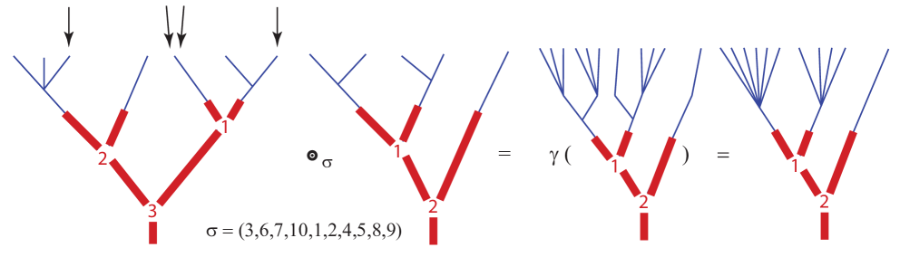
Figure 25. One term in the product defined in Section 3, relative to the given shuffle.

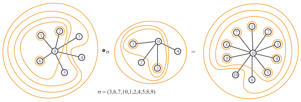
Figure 26. The same product as pictured in Figure 25, shown here using tubings on the star graphs.

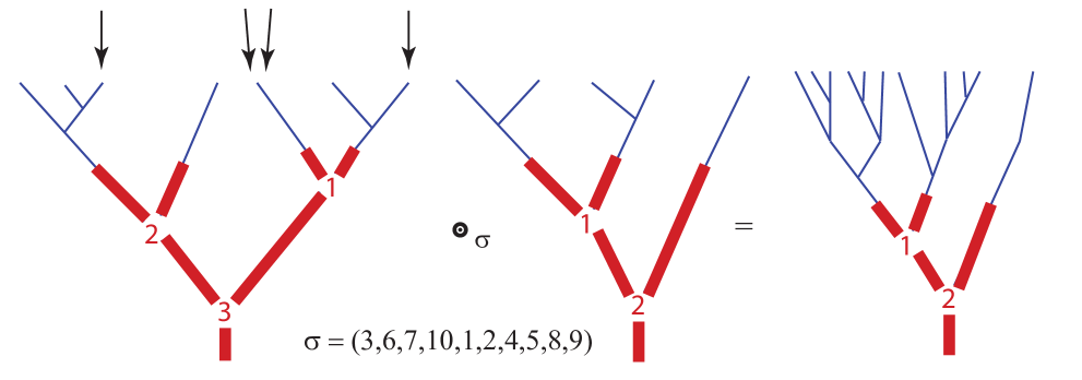
Figure 27. One term in the product defined in Section 3, relative to the given shuffle.

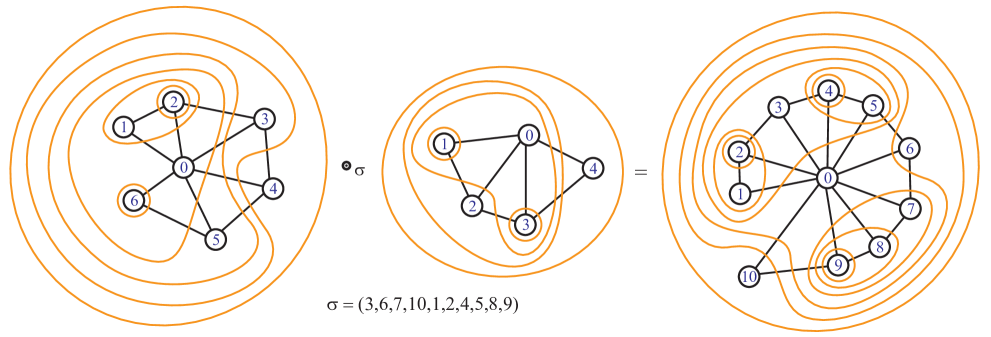
Figure 28. The same product as pictured in Figure 27, shown here using tubings on the star graphs.

6. Alternative product on the Stellohedra vertices

For $n\geq 1$, we denote by $[n]$ the set $\{1,\dots,n\}$. For any set of natural numbers $U=\{u_{1},\dots,u_{k}\}$ and any integer $r\in{\mathbb{Z}}$, we denote by $U+r$ the set $\{u_{1}+r,\dots,u_{k}+r\}$.

Let $G$ be a simple finite graph with set of nodes ${\mbox{Nod}(G)}=\{j_{1},\dots,j_{r}\}\subseteq{\mathbb{N}}$, we denote by $G+n$ the graph $G$, with the set of nodes colored by ${\mbox{Nod}(G)}+n$, obtained by replacing the node $j_{i}$ of $G$ by the node $j_{i}+n$, for $1\leq i\leq r$.

Let $G$ be a simple finite graph, whose set of nodes is $[n]$, we identify a tube $t=\{v_{1},\dots,v_{k}\}$ of $G$ with the tube $t(h)=\{v_{1}+h,\dots,v_{k}+h\}$ of $G+h$. For any tubing $T=\{t_{i}\}$ of $G$, we denote by $T(h)$ the tubing $\{t_{i}(h)\}$ of $G+h$.

In the present section, we use the shuffle product, which defines an associative structure on the vector space spanned by all the vertices of permutohedra, in order to introduce associative products (of degree ${-}1$) on the vector spaces spanned by the vertices of stellohedra.

Definition 6.1.

Let $T$ be a maximal tubing of $\mbox{St}_{n}$ and ${V}$ be a maximal tubing of $\mbox{St}_{m}$ such that $T={\mbox{Tub}_{r}(u_{1},\dots,u_{n})}$ and $V={\mbox{Tub}_{s}(v_{1},\dots,v_{m})}$. For any $(n-r,m-s)$- shuffle $\sigma\in S_{n+m{-}r{-}s}$ define the maximal tubing $T*_{\sigma}{V}$ of $S_{n+m}$ as follows:

$$T*_{\sigma}{V}:={\mbox{Tub}_{r+s}(u_{1},\dots,u_{r},v_{1}{+n},\dots,v_{s}{+n},w_{\sigma^{-1}(1)},\dots,w_{\sigma^{-1}(n+m{-}(r+s))})},$$

where:

$$w_{i}:=\left\{\begin{array}[]{lr}u_{r+i},\ {\rm for}\ 1\leq i\leq n-r,\\ v_{s+i+r{-}n}{+n},\ {\rm for}\ n-r<i\leq n+m-r-s.\end{array}\right\}$$

If $T={\mbox{Tub}_{n}}$, then $\sigma=1_{m}$ and

$${\mbox{Tub}_{n}}*_{1_{m}}{V}={\mbox{Tub}_{n+s}(1,\dots,n,v_{1}+n,\dots,v_{m}+n)}.$$

In a similar way, we have that

$$T*_{1_{n}}{\mbox{Tub}_{m}}={\mbox{Tub}_{r+m}(u_{1},\dots,u_{r},n+1,\dots,n+m,u_{r+1},\dots,u_{n})}.$$

In Figure 29 we illustrate the following example.

$${\mbox{Tub}_{3}(1,2,6,5,3,4)*_{\sigma}\mbox{Tub}_{2}(1,3,2,4)}=\mbox{Tub}_{5}(1,2,6,7,9,5,8,3,10,4)$$

…where $\sigma=(1,3,5,2,4).$ For comparison see a product with the same operands in Figure 26.

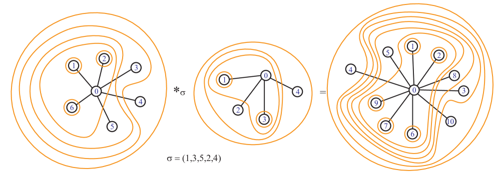
Figure 29. Example of Definition 6.1.

Using Definition 6.1, we define a shuffle product on the vector space ${\mathbb{K}}[{\mathcal{MT}}(\mbox{St})]:=\bigoplus_{n\geq 1}{\mathbb{K}}[{\mathcal{MT}}(\mbox{St}_{n})]$, where ${\mathcal{MT}}(\mbox{St}_{n})$ denotes the set of maximal tubings on $\mbox{St}_{n}$, which correspond to the vertices of stellohedra, as follows.

Definition 6.2.

Let $T\in{\mathcal{MT}}(\mbox{St}_{n})$ and ${V}\in{\mathcal{MT}}(\mbox{St}_{m})$ be two maximal tubings. The product $T*{V}\in{\mathcal{MT}}(\mbox{St}_{n+m})$ is defined as follows:

1. If $T={\mbox{Tub}_{r}(u_{1},\dots,u_{n})}\neq{\mbox{Tub}_{n}}$ and ${V}={\mbox{Tub}_{s}({v}_{1},\dots,{v}_{m})}\neq{\mbox{Tub}_{m}}$, then:

   $$T*{V}:=\sum_{\sigma\in{\mbox{Sh}(n-r,m-s)}}T*_{\sigma}{V},$$

   where ${\mbox{Sh}(n-r,m-s)}$ denotes the set of $(n{-}r,m{-}s)$-shuffles in $S_{n+m{-}(r+s)}$.

2. If $T={\mbox{Tub}_{n}}$ and ${V}={\mbox{Tub}_{m}}$, then:

   $$T*{V}={\mbox{Tub}_{n+m}}.$$

3. If $T={\mbox{Tub}_{n}}$ and ${V}={\mbox{Tub}_{s}({v}_{1},\dots,{v}_{m})}\neq{\mbox{Tub}_{m}}$, then:

   $$T*{V}:={\mbox{Tub}_{n+s}(1,\dots,n,{v}_{1}+n,\dots,{v}_{m}+n)}.$$

4. If $T={\mbox{Tub}_{r}(u_{1},\dots,u_{n})}\neq{\mbox{Tub}_{n}}$ and ${V}={\mbox{Tub}_{m}}$, then:

   $$T*{V}:={\mbox{Tub}_{r+m}(u_{1},\dots,u_{r},n+1,\dots,n+m,u_{r+1},\dots,u_{n})}.$$

Proposition 6.3.

The graded vector space ${\mathbb{K}}[{\mathcal{MT}}(\mbox{St})]$, equipped with the product $*$ is an associative algebra.

Proof.

Suppose that the elements $T={\mbox{Tub}_{r}(u_{1},\dots,u_{n})}$ in ${\mathcal{MT}}(\mbox{St}_{n})$, $V={\mbox{Tub}_{s}(v_{1},\dots,v_{m})}$ belongs to ${\mathcal{MT}}(\mbox{St}_{m})$ and $W={\mbox{Tub}_{z}(w_{1},\dots,w_{p})}$ belongs to ${\mathcal{MT}}(\mbox{St}_{p})$ are three maximal tubings, where eventually $T={\mbox{Tub}_{n}}$, $V={\mbox{Tub}_{m}}$ or $W={\mbox{Tub}_{p}}$.

Applying the associativity of the shuffle, we get that:

$$\begin{array}[]{lr}(T*V)*W=\\ &\sum{\mbox{Tub}_{r+s+z}(u_{1},\dots v_{r},v_{1}{+n},\dots,w_{1}{+n+m},\dots,x_{\sigma^{-1}(1)},\dots,x_{\sigma^{-1}(n+m+p{-}(r+s+z))})}\\ ~{}~{}~{}~{}~{}~{}~{}~{}~{}~{}~{}~{}~{}~{}~{}~{}~{}~{}=T*(V*W),\end{array}$$

where we sum over all permutations $\sigma\in{\mbox{Sh}(n{-}r,{m}-s,p{-}s)}$ and

$$x_{i}:=\left\{\begin{array}[]{lr}u_{r+i},&{\rm for}\ 1\leq i\leq n{-}r,\\ v_{s+i+r{-}n}{+n},&{\rm for}\ n{-}r<i\leq n+m{-}r{-}s,\\ w_{z+i+r+s{-}n{-}m}{+n+m},&{\rm for}\ n+m{-}r{-}s<i\leq n+m+p{-}r{-}s{-}z,\end{array}\right\}$$

which ends the proof. ∎

7. Questions

There are well-known extensions of $\mathfrak{S}\mathit{Sym}$ and $\mathcal{Y}Sym$ to Hopf algebras based on all of the faces of the permutohedron and associahedron. These were first described by Chapoton, in [8], along with a Hopf algebra of the faces of the hypercubes. We realize the first two Hopf algebras using the graph tubings in [17]. They are denoted $\mathfrak{S}S\widetilde{ym}$ and $\mathcal{Y}S\widetilde{ym}$ respectively, and so we refer to Chapoton’s algebra of the faces of the cube as $\mathfrak{C}S\widetilde{ym}$.

Immediately the question is raised: how might we relate the coalgebra $\mathfrak{S}S\widetilde{ym}\circ\mathfrak{C}S\widetilde{ym}$ to our algebra of stellohedra faces? How can we relate the Hopf algebra on $\widetilde{C/C}$ for $C$ the corollas, thus an algebra on the faces of the hypercube, to Chapoton’s Hopf algebra $\mathfrak{C}S\widetilde{ym}$?

Further questions arise as we look at the other polytopes in our set of 12 sequences. (Of course, recall that 4 of them are only conjecturally convex polytope sequences.) For instance, via our bijection there is a Hopf algebra based on the weakly ordered forests grafted to corollas–which we would like to characterize in terms of known examples.

8. Acknowledgements

The authors thank a referee who made many good suggestions about an early version. The third author is supported via Fondecyt Regular, Project 1171209. The second author would like to thank the AMS and the Mathematical Sciences Program of the National Security Agency for supporting this research through grant H98230-14-0121. The second author’s specific position on the NSA is published in [12]. Suffice it to say here that the second author appreciates NSA funding for open research and education, but encourages reformers of the NSA who are working to ensure that protections of civil liberties keep pace with intelligence capabilities.

References

- [1] Marcelo Aguiar and Frank Sottile. Structure of the Malvenuto-Reutenauer Hopf algebra of permutations. Adv. Math., 191(2):225–275, 2005.
- [2] Marcelo Aguiar and Frank Sottile. Structure of the Loday-Ronco Hopf algebra of trees. J. Algebra, 295(2):473–511, 2006.
- [3] Federico Ardila and Jeffrey Doker. Lifted generalized permutahedra and composition polynomials. Advances in Applied Mathematics, 50:607–633, 2013.
- [4] P. Barry. A Catalan transform and related transformations on integer sequences. Journal of Integer Sequences, 8(2):3, 2005.
- [5] F. Bergeron, P. Leroux, and G. Labelle. Combinatorial Species and Tree-like Structures. Encyclopedia of Mathematics. Cambridge University Press, 1998.
- [6] J. M. Boardman and R. M. Vogt. Homotopy invariant algebraic structures on topological spaces. Lecture Notes in Mathematics, Vol. 347. Springer-Verlag, Berlin, 1973.
- [7] Michael P. Carr and Satyan L. Devadoss. Coxeter complexes and graph-associahedra. Topology Appl., 153(12):2155–2168, 2006.
- [8] Frédéric Chapoton. Bigèbres différentielles graduées associées aux permutoèdres, associaèdres et hypercubes. Ann. Inst. Fourier (Grenoble), 50(4):1127–1153, 2000.
- [9] Satyan Devadoss and Stefan Forcey. Marked tubes and the graph multiplihedron. Algebr. Geom. Topol., 8(4):2081–2108, 2008.
- [10] Satyan L. Devadoss. A realization of graph associahedra. Discrete Math., 309(1):271–276, 2009.
- [11] Satyan L. Devadoss, T. Heath, and C. Vipismakul. Deformations of bordered surfaces and convex polytopes. Notices of the AMS, 58(1):530–541, 2011.
- [12] S. Forcey. Dear NSA: Long-term security depends on freedom. Notices of the AMS, 61(1), 2014.
- [13] Stefan Forcey. Convex hull realizations of the multiplihedra. Topology Appl., 156(2):326–347, 2008.
- [14] Stefan Forcey, Aaron Lauve, and Frank Sottile. New hopf structures on binary trees. DMTCS Proc. FPSAC 21, pages 411–420, 2009.
- [15] Stefan Forcey, Aaron Lauve, and Frank Sottile. Cofree compositions of coalgebras. Ann. Comb., 17(1):105–130, 2013.
- [16] Stefan Forcey and Derriell Springfield. Geometric combinatorial algebras: cyclohedron and simplex. preprint.
- [17] Stefan Forcey and Derriell Springfield. Geometric combinatorial algebras: cyclohedron and simplex. J. Alg. Combin., 32(4):597–627, 2010.
- [18] Jean-Louis Loday and María O. Ronco. Hopf algebra of the planar binary trees. Adv. Math., 139(2):293–309, 1998.
- [19] Jean-Louis Loday and María O. Ronco. Order structure on the algebra of permutations and of planar binary trees. J. Alg. Combinatorics, 15:253–270, 2002.
- [20] Jean-Louis Loday and María O. Ronco. Trialgebras and families of polytopes. In Homotopy theory: Relations with Algebraic Geometry, Group Cohomology and Algebraic -Theory, volume 346 of Contemp. Math., pages 369–398. Amer. Math. Soc., Providence, RI, 2004.
- [21] Clauda Malvenuto and Christophe Reutenauer. Duality between quasi-symmetric functions and the Solomon descent algebra. J. Algebra, 177(3):967–982, 1995.
- [22] Thibault Manneville and Vincent Pilaud. Compatibility fans for graphical nested complexes. Journal of Combinatorial Theory, Series A, 150:36–107, 2017.
- [23] Vincent Pilaud. Signed tree associahedra. DMTCS Proc. FPSAC 26, pages 309–320, 2014.
- [24] Alex Postnikov, Victor Reiner, and Lauren Williams. Faces of generalized permutohedra. Doc. Math., 13:207–273, 2008.
- [25] Alexander Postnikov. Permutohedra, associahedra, and beyond. Int. Math. Res. Not. IMRN, (6):1026–1106, 2009.
- [26] N. J. A. Sloane. The on-line encyclopedia of integer sequences. published electronically at www.oeis.org.
- [27] Andy Tonks. Relating the associahedron and the permutohedron. In Operads: Proceedings of Renaissance Conferences (Hartford, CT/Luminy, 1995), volume 202 of Contemp. Math., pages 33–36. Amer. Math. Soc., Providence, RI, 1997.
- [28] E. Zoque. Partitions, pairs of trees and Catalan numbers. arXiv preprint arXiv:1006.5706, 2010.