A PSF-based approach to Kepler/K2 data – III. Search for exoplanets and variable stars within the open cluster M 67 (NGC 2682)

Abstract

In the third paper of this series we continue the exploitation of Kepler/K2 data in dense stellar fields using our PSF-based method. This work is focused on a $\sim 720$-arcmin² region centred on the Solar-metallicity and Solar-age open cluster M 67. We extracted light curves for all detectable sources in the Kepler channels 13 and 14, adopting our technique based on the usage of a high-angular-resolution input catalogue and target-neighbour subtraction. We detrended light curves for systematic errors, and searched for variables and exoplanets using several tools. We found 451 variables, of which 299 are new detection. Three planetary candidates were detected by our pipeline in this field.

Raw and detrended light curves, catalogues, and K2 stacked images used in this work will be released to the community.

1 Introduction

The data collected during the reinvented Kepler/K2 mission (Howell et al. 2014) allowed the community to search for new variable stars and exoplanets in many Galactic fields, containing various kinds of objects (single stars, open and globular clusters, extra-galactic sources, etc.). Despite the lower quality of K2 data compared to Kepler main mission, many techniques for the extraction and the systematic correction of the light curves (LCs) have been developed in these last two years.

Libralato et al. (2016b, hereafter Paper I) developed a new tool to extract high photometric precision LCs from the K2 undersampled images of crowded environments, based on the usage of effective Point Spread Functions (ePSFs) and of a high-angular-resolution input catalogue. However this approach is perfectly suitable for any stellar field. This PSF-based technique also allows us to extract LCs for sources in the faint magnitude regime ($K_{\rm P}>15.5$), increasing the number of analysable objects in a field.

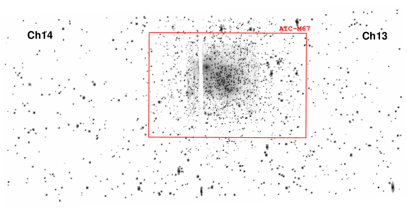
Figure 1: Field of view covered by all available K2/C5 Ch13 (right) and Ch14 (left) exposures used in our analysis. The red rectangle represents the field of view covered by the AIC-M67 (Nardiello et al. 2016). The image is in logarithmic grey scale. North is up and East to the left.

In this work we take advantage of this method, focusing our attention on the moderate-crowded region containing the open cluster (OC) M 67 (NGC 2682). During the K2 Campaign 5 (K2/C5), two super-stamps (covering a region between two Kepler channels of module 6) centred on M 67 were achieved. We reconstructed all the images containing the super-stamps and applied our PSF-based approach to extract high-precision LCs.

The OC M 67 is one of the most studied and intriguing OCs in literature (see, e.g., Nardiello et al. 2016 and references therein). This OC has an age and metallicity similar to that of the Sun (e.g., Bellini et al. 2010; Heiter et al. 2014) and is located at a distance $<1$ kpc (Pandey et al. 2010). In a previous paper based on ground-based, Asiago Schmidt data (Nardiello et al. 2016), we have already investigated this OC, detecting 43 new variables. In this work, we used the same input catalogue to extract LCs from the K2/C5 images, and search for new variable stars among M 67 members.

Together with M 44 (Quinn et al. 2012; Malavolta et al. 2016) and the Hyades (Quinn et al. 2014), M 67 is one of the few OCs that host stars with confirmed exoplanets. Brucalassi et al. (2014, 2016), using radial velocity (RV) measurements, have detected four exoplanets orbiting M 67 members, three of which are main sequence (MS) stars. In this work we conducted a search for transiting planets on all M 67 member (and not) stars, in order to identify low-mass planets that could have been overlooked by RV searches.

2 Observations and data reduction

The K2 observations were performed during C5. The data-set includes 3620 usable long-cadence observations, that spanned over 74.82 days (April 27th - July 10th, 2015).

The bulk of M 67 falls in between the two KEPLERCAM channels 13 (Ch13) and 14 (Ch14) of module 6. In this work we focus exclusively on the point sources monitored by K2/C5 on these two channels.

In each channel a super-stamp was monitored. The one in Ch14 is 90$\times$400 pixels², while the one of Ch13 is larger, with 312$\times$400 pixels². Overall the two super-stamps would continuously cover a region of $402\times 400$ pixels² ($\sim 0.2$ degree²) centred on the M 67’s centre (see Fig. 1) without considering the gap between the two channels. We have analysed as well the individual postage stamps present in both channels.

We downloaded the K2 Target Pixel Files (TPFs) containing the complete time series data from the “Mikulski Archive for Space Telescopes” (MAST). We reconstructed the 3620 images ($1132\times 1070$ pixel²) of the series for each channel, one for each cadence number of the TPFs. We assigned to each pixel the sum of the values of the columns FLUX and FLUX_BKG. To each image we assigned the average Kepler Barycentric Julian Day (KBJD) corresponding to the KBJD associated to the cadence number.

In the following we give a brief summary of the LC extraction, that was carefully described in Paper I. Our method for the LC extraction essentially relies on:

1. time-perturbed effective PSFs (ePSFs),

2. a high-angular-resolution stellar input catalogue,

3. six-parameters, local linear transformations between single-image catalogues and the input catalogue,

4. neighbour subtraction.

2.1 Improved PSFs

In Paper I we have described how to model the undersampled PSF of Kepler using the recipe by Anderson & King (2000). In this work we used a slightly improved version of the ePSFs obtained with the method described in Paper I. The method will be explained in detail in a future paper of the series focus on M 4 (Libralato et al. in preparation). It differs from that presented in Paper I only in the fact that neighbours are iteratively subtracted (using the current ePSF model and an input list) to the sample stars used to define the ePSF model and imposing the positions of the used stars from the input list before computing the new improved ePSF models.

2.2 The Asiago Input Catalogue for M 67 (AIC-M67)

We used as input catalogue the Asiago Schmidt catalogue of M 67 released by Nardiello et al. (2016), hereafter AIC-M67. This catalogue, obtained using Asiago Schmidt 67/92 cm data, gives positions, magnitudes in 8 filters, proper motions and membership probabilities for 6905 sources in a field of $58\times 38$ arcmin² centred on M 67 cluster centre. The coverage of this input catalogue is shown in Fig. 1 (red rectangle).

2.3 The K2-Stacked-Image Catalogues (K2S-Ch13/-Ch14)

Many M 67 stars are located in postage stamps recorded by K2/C5 outside the AIC-M67 region in both channels (see Fig. 1), hence the need of extending the AIC-M67. For each channel we made a stacked image using all 3620 usable images, as described in Paper I. Then, we applied the same procedure adopted on single images to extract the catalogues from the stacked images, excluding all sources that fell inside the AIC-M67 region. For the Ch13 and Ch14, we created two additional input catalogues: the K2’s Stacked-Image Ch13 (hereafter K2S-Ch13) containing 437 additional stars, and the K2S-Ch14 with 328 additional stars. For each channel, the final input list adopted was a merge between the AIC-M67 and K2S-Ch13 or K2S-Ch14 catalogue.

3 Light Curve extraction

For the extraction of the LCs, we used the software developed and described by Nardiello et al. (2015) for the ground-based telescope Asiago Schmidt 67/92 cm and adapted in Paper I for K2 data.

Given a target star in the input catalogue, the software locally transforms positions and magnitudes of all its input catalogue neighbours (inside a radius of 35 Kepler pixels, i.e., $\sim 2.3$ arcmin) from the reference system of the input catalogue into that of the individual K2 image. Next, we subtracted these target neighbours from the considered image. We extracted the flux of the target source from the original and the neighbour-subtracted images, using three methods: (i) PSF-fitting, (ii) aperture, and (iii) optimal-mask photometry. For aperture photometry we used four different apertures: 1-, 2.5-, 3.5-, and 4.5- pixel radii. For optimal-mask photometry, in analogy with Vanderburg & Johnson (2014), we used two different masks based on the ePSF model: for the first mask (mask-1), suitable for bright stars ($K_{\rm P}<13$), are considered only pixels for which the normalised ePSF value is $\geq 0.005$%; the second mask (mask-2), suitable for fainter stars, is made by pixels for which the ePSF value is $\geq 0.1$%.

We have already demonstrated in Paper I that the photometric precision is better for neighbour-subtracted photometries; for this reason, hereafter, we will only consider neighbour-subtracted LCs.

3.1 Light Curve detrending

The larger jitter of the spacecraft pointing during the K2-mission (if compared to that of the Kepler main mission) translates into a worse photometric precision. To correct the most of the systematic errors, that are related to the spacecraft drift, several methods appeared in the literature. In this work we used the same detrending algorithm presented in Paper I for the K2/C0 Ch81 data, slightly improved adding a new step, that proved to be effective in taking into account the specifics of each campaign.

Already in the original Kepler mission the LCs show some systematic effects not correlated with the positions and the magnitude of the stars on the detectors, but associated with spacecraft, detector and environment (Christiansen et al. 2013). During a K2 campaign, all stars in the same channel show common systematic trends in their LCs. This particular behaviour allows to model these systematic trends as a linear combination of orthonormal functions, called cotrending basis vectors (CBVs). In an analogous way as the Kepler standard pipeline for the LC reduction, we used the publicly available CBVs (released by the Kepler team) for modelling and correcting these systematic features.

Given a raw LC normalised to its median flux, as that shown in panel (a) of Fig. 2 (star # 7187 in the input catalogue of Ch13, EPIC 211380061), and the CBV_i, with $i=1,...,16$, our routine finds the coefficients $A_{i}$ that minimise the expression:

$$F_{\rm raw}^{j}-\sum_{i}\left(A_{i}\cdot{\rm CBV}_{i}^{j}\right)$$ (1)

where $F_{\rm raw}^{j}$ is the raw flux at time $j$, $j=1,...,N_{\rm epochs}$, and $N_{\rm epochs}$ is the number of points in the LC. For the minimisation, we used the Levenberg-Marquardt method (Moré et al. 1980). In panel (b) of Fig. 2 we show the cotrended LC. It is clear that most of the systematic effects are corrected.

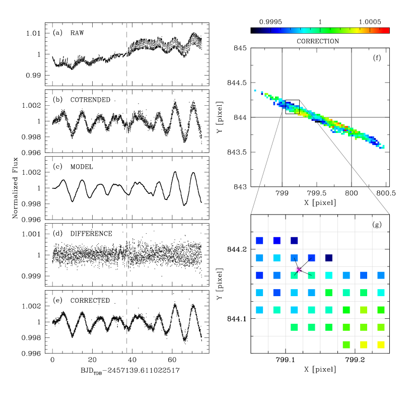
Figure 2: Overview of the procedure used for correcting the 3.5-pixel-aperture LC of star Ch13-#7187 (EPIC 211380061). Panels from (a) to (e) show the procedure for obtaining the systematic-corrected LC starting from the raw LC. Dashed grey line is the boundary line between the two segments in which the LC has been splitted during the detrending phase. In panel (f) we show cell and grid-point locations around the star Ch13-#7187 loci on the Ch13 over the entire K2/C5. The coloured cells (size $0.025\times 0.025$-pixel² each) represent the correction applied to the flux at a given $(x,y)$ position. The black-square region is zoomed in panel (g): for a $(x,y)$ position at a given time (magenta asterisk), the correction is computed by using a bi-linear interpolation of the four surrounding grid points (see text for details). We excluded the points associated to thruster-jet from the LCs plotted in panels (a)-(e).

After cotrending the LCs, we detrend them for residuals systematic errors using the same procedure as described in detail in Paper I. This method consists in a 2D self flat-fielding, similar to existing techniques developed by others, but that takes advantage of our high-precision positioning, a result of our careful ePSF modelling and of the local-transformations approach between the input list and the single-image catalogues.

For each target star, we modelled its median-normalised-flux LC in order to disentangle the true intrinsic stellar variability from the systematic errors above described. In order to obtain the model, we divided the LC in $N-1$ segments (where $N$ is the number of thruster firings during the entire campaign). Each segment contained the photometric points collected between two consecutive spacecraft thruster firings. We have identified the “break-points” between two segments thanks to the variations of the target positions $\left(X,Y\right)$. In each segment we calculated the $3.5\sigma$-clipped average of the photometric points, obtaining $N$ knots. We obtained the final model of the intrinsic variability by a linear interpolation of the knots over the observing time (panel c of Fig. 2).

After correcting for the intrinsic variability, the model-subtracted LC reflected the systematic effect originated by the motion of the star on the detector (panel d of Fig. 2). This is corrected according with Paper I recipes. Briefly, we divided the pixels “touched” by the target star into an array of $40\times 40$ cells. We filled the grid by computing the $3.5\sigma$-clipped median of the LC flux in each element of the grid (panel f of Fig. 2). For each $\left(x,y\right)$ position on the CCD, the correction is given by the bi-linear interpolation between the 4 closest grid points, as shown in panel (g) of Fig. 2. After different tests, we found that for M 67 K2/C5 LCs the best detrending was achieved by splitting the time-series in two distinct segments (the boundary between the two LC segments is marked by a dashed grey lines in panels a-e of Fig. 2, corresponding to $\sim 37.2$ days after the beginning of the campaign). Our detrending is an iterative procedure, in such a way that both the model for the intrinsic variability and the spacecraft drift are improved at each step. The corrected LC is shown in panel (e) of Fig. 2. This correction is far from being perfect and it could be considered only preliminary. For example, the cotrend stage works well for a large sample of LCs, but there are variable stars for which the use of all the 16 CBVs is not the best solution. Indeed, the best solution is an ad-hoc combination of CBVs for each LC that both preserves the intrinsic stellar variability and gives the higher photometric precision. Since we checked that a large part of stellar LCs in our sample preserves their intrinsic signals, we postpone the development of new LC-correction techniques to future works. We release the raw LCs to the community to stimulate the development of independent detrending algorithms that could be tested in the meantime.

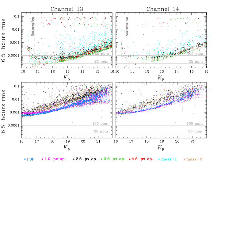
Figure 3: The 6.5h-rms for PSF-fitting (azure), 1-pixel-aperture (magenta), 2.5-pixel-aperture (black), 3.5-pixel-aperture (green), 4.5-pixel-aperture (red), mask-1 (cyan), and mask-2 (brown) photometry on the neighbour-subtracted LCs. Top-panels show the 6.5h-rms for stars with $K_{\rm P}<16$ and for 2.5-pixel-aperture (black), 3.5-pixel-aperture (green), 4.5-pixel-aperture (red), and mask-1 (cyan) photometry; bottom panels for $K_{\rm P}\geq 16$ and PSF-fitting (azure), 1-pixel-aperture (magenta), 2.5-pixel-aperture (black), and mask-2 (brown) photometry. Stars of Ch13 and Ch14 are plotted in left and right panels, respectively. The grey, solid horizontal lines are located at 100 and 25 ppm, while vertical dashed lines indicate the saturation limit ( $K_{\rm P}\sim 10.8$ ).

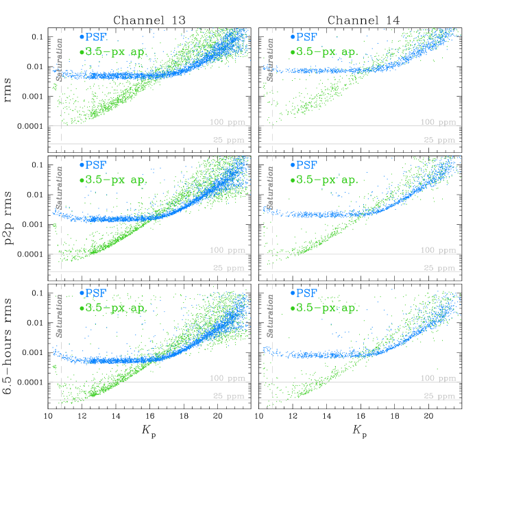
Figure 4: Photometric-precisions comparison between PSF-fitting (azure) and 3.5-pixel-aperture (green) photometry, that are, on average, the best solution in the faint- and bright-magnitude regime, respectively. From top to bottom: simple rms, p2p rms, and 6.5h-rms. Left and right panels show the rms for Ch13 and Ch14 stars, respectively. Solid, horizontal lines are set at 25 and 100 ppm. Vertical dashed lines indicate the saturation threshold.

3.2 Photometric Calibration

We calibrated our catalogues into Kepler Magnitude System ($K_{\rm P}$) by comparing the average PSF-fitting instrumental magnitudes of unsaturated stars with the $K_{\rm P}$-magnitudes of the same stars in the Ecliptic Plane Input Catalog (EPIC). We used the EPIC $K_{\rm P}$ magnitudes obtained from $gri$ photometry, as done in Section 5 of Paper I. We found a median difference in zero-point of 25.31$\pm$0.07 for Ch13 and 25.17$\pm$0.06 for Ch14.

3.3 Photometric precision

As in Paper I, we extracted three different parameters to analyse the photometric precision:

1. rms: we have defined this quantity as the $3.5\sigma$-clipped 68.27th-percentile of the distribution around the median value of the points in the LC;

2. point-to-point (p2p) rms: for each LC, we have computed the quantity $\delta F_{j}=\lvert F_{j}-F_{j+1}\rvert$, with $F_{j}$ and $F_{j+1}$ the flux values at times $j$ and $j+1$, with $j=1,...,N_{epochs}-1$. We have defined the p2p rms as the $3.5\sigma$-clipped 68.27th-percentile of the distribution around the median value of $\delta F$.

3. 6.5-hour rms: we applied to each LC a 6.5h-running average filter. We divided the processed LC in bins containing 13 points. For each bin, we computed the $3.5\sigma$-clipped rms and divided it by $\sqrt{12}$. We have defined the 6.5h rms as the median value of these rms measurements.

In Fig. 3 we show a comparison between the 6.5h-rms of the different adopted photometric methods for bright (top panels) and faint (bottom panels) stars, and for stars in Ch13 (left panels) and Ch14 (right panels). On average, mask-1 gives the best LCs for saturated stars ($K_{\rm P}\lesssim 10.8$), even if lower rms are associated to 4-pixel aperture photometry. Bright, unsaturated stars ($10.8\lesssim K_{\rm P}\lesssim 12.5$) are well measured with the 4-pixel aperture photometry (lowest 6.5h-rms $\sim$ 13.5 ppm), while 2.5- and 3.5-pixel aperture photometric methods are the best solution for stars with $12.5\lesssim K_{\rm P}\lesssim 16$. In the faint regime of magnitude ($K_{\rm P}\gtrsim 16$) 1-pixel aperture, mask-2 and PSF-fitting photometric methods give the best photometric precision.

In Fig. 4 we show the simple rms, the p2p rms, and the 6.5h-rms for 3.5-pixel aperture and PSF-fitting photometric methods, that are, on average, the best solution for bright and faint stars, respectively.

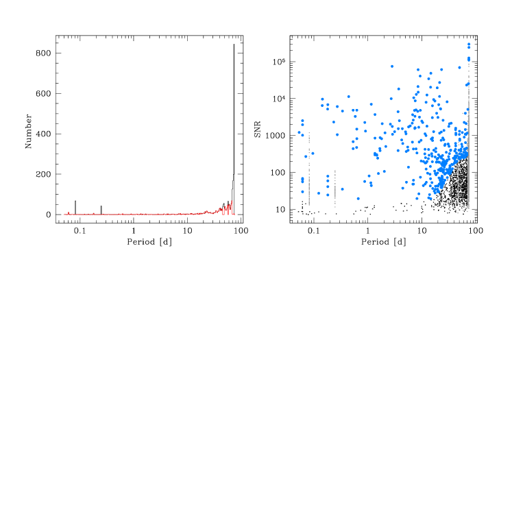
Figure 5: Example of candidate-variable selection using the AoV algorithm (for stars in Ch13). Left Panel: distribution of the periods before (black) and after (red) spikes suppression. Right Panel: the AoV SNR as a function of the period before (grey) and after the spike suppression (black). In azure the variable candidates.

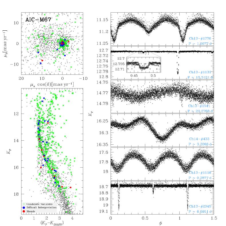
Figure 6: Overview of the variability-finding results. Bottom-left panel: $K_{\rm P}$ versus $(K_{\rm P}-K_{\rm 2MASS})$ CMD of M 67; the red dots are the blends, the green crosses the candidate variables, and the blue dots the stars difficult to interprete. Top-left panel: Vector-point diagram of proper motions (from Nardiello et al. 2016) for the same stars plotted in the CMD, colour-coded as in bottom-left panel. Right panels: a few examples of variable stars in order of decreasing magnitudes from top to bottom.

4 Variable stars

Variable-star detection has been performed using the method described by Nardiello et al. (2015, 2016) and also used in Paper I and Libralato et al. (2016a, hereafter Paper II).

First, we cleaned the LCs from the bad points due to bad-pixels, cosmic-rays, etc, dividing the LC in bins of 0.2 days, computing the LC median and $\sigma$ values in each bin and clipping the points that are 3.5$\sigma$ brighter or 15$\sigma$ fainter than the median value. In this way we clipped-out a large part of the outliers, but preserved the eclipsing/transits of eclipsing binaries and/or planets. We also excluded all the thruster-jet-related events from the LC, as done in Paper I.

We used three different algorithms (that are part of VARTOOLS v. 1.33, Hartman & Bakos 2016) on the clean LCs in order to detect variable stars: the Generalised Lomb-Scargle (GLS) periodogram (Zechmeister & Kürster 2009), the Analysis of Variance (AoV) periodogram (Schwarzenberg-Czerny 1989), and the Box-fitting Least-Squares (BLS) periodogram (Kovács et al. 2002). Using all these tools it is possible to detect all kind of variable stars (sinusoidal, irregular, eclipsing binaries, etc.). Figure 5 summarises the procedure used to isolate candidate variable stars using the AoV method. The procedure is the same in the case of GLS and BLS. Briefly, from the histograms of the detected periods for all the LCs, we removed the spikes associated to spurious periods due to systematic effects. Left panel of Fig. 5 shows the histogram before (black) and after (red) the spike suppression. Right panel of Fig. 5 shows the AoV Signal-to-noise ratio (SNR) as a function of the detected periods, in grey and in black before and after the spikes suppression, respectively. In this plot we selected by hand the stars having high SNR. These points refer to stars with high probability to be variable (azure points). We performed the same analysis for GLS and BLS method outputs. In the case of BLS periodograms we used as diagnostic the Signal-to-Pink noise. Finally, we visually inspected each of them in order to obtain the final catalogue. From this catalogue, we excluded all the obvious blends by comparing the shape and the period of each candidate-variable LC with that of its neighbours (within 20 K2 pixels).

Among a total of 4142 stars (Ch13 and Ch14) for which we have extracted a reliable LC, we have found 318 and 170 candidate variables for Ch13 and Ch14, respectively, for a total of 488 candidate variables. Among these candidates, we have flagged 11 stars as obvious blends and 26 stars as difficult to interprete. In the difficult-interpretation sample there are sources that could be real variable stars, blends or stars with residual systematic effects that mime a fake variability.

In left panels of Fig. 6 we show the $K_{\rm P}$ versus $(K_{\rm P}-K_{\rm 2MASS})$ colour-magnitude diagram (CMD) of all stars in the field (bottom) and the vector-points diagram of stellar proper motions (top panel, from Nardiello et al. 2016 catalogue). The green crosses identify the candidate variables, the blue dots the difficult-interpretation objects and the red dots the obvious blends.

Finally we have cross-matched our catalogue of candidate variable stars with the available catalogues in literature. We considered only the 451 surely not blended stars, and we find that 152 of them have already been catalogued by Gilliland et al. (1991), Stassun et al. (2002), van den Berg et al. (2002), Sandquist & Shetrone (2003a, b), Stello et al. (2006), Stello et al. (2007), Bruntt et al. (2007), Pribulla et al. (2008), Yakut et al. (2009), Nardiello et al. (2016), and Gonzalez (2016). Therefore, in our catalogue there are 299 new variable stars. Examples of variables in our catalogue are given in right panels of Fig. 6.

5 Candidate Exoplanet transits

To search for candidate-exoplanet transits, we used the procedure described in detail in Paper II. In the following we give a short description of our pipeline.

For each star, we flattened and cleaned its LC by modelling the stellar intrinsic variability with a $k^{\rm th}$-order spline with $N$ break points, removing out the outliers as described in the previous section. To take into account different kind of variability, we performed the analysis using three different combinations of $k$ and $N$: $k=3$ and $N=75$, $k=3$ and $N=150$, and $k=5$ and $N=175$.

For each flat/cleaned LC we extracted the BLS periodogram and we normalised it as in Vanderburg et al. (2016), in order to minimise the long-period false detection. We selected the five most significant peaks in the normalised BLS periodogram, excluding the harmonics of each peak and the spurious signals related to the instrumentation.

For each of the five periods found, we used BLS again to refine the central time and the duration of the candidate transit. We phased the flat LC and checked if the transit flux drop was at least one $\sigma$ below the out-of-transit level. Then, we verified whether there were or not other similar flux drops in the phased LC (e.g., due to an EB). Finally, we visually inspected the candidate transits that passed the previous checks to exclude false alarms.

Excluding the obvious, already catalogued EBs and false alarms, we found 5 interesting objects: 2 are EBs in the M 67 field that, without a proper analysis, could be mistaken for transiting-planet host; the other 3 are candidate exoplanets. We present them in the next sections.

5.1 Eclipsing binaries

5.1.1 Star Ch13-#1679

The first object of interest is star Ch13-#1679 (EPIC 211415154, also known as HX Cnc or S1070, Sanders 1977). Figure 7 shows an overview of its LC: top-left panel shows the flattened LC, while the top-right panel reproduces the LC phased with the period found by the AoV periodogram (P$\sim$2.62 d). This is the period related to the activity of the principal component. We flattened and cleaned the LC using a $5^{\rm th}$-order spline with 175 break points, and clipped out the outliers. The flattened-cleaned LC is shown in the middle-left panel, while in the middle-right panel the phased LC is plotted with the period (P$\sim$2.66 d) found by our pipeline. A careful analysis of the phased LC reveals that, in addition to the minimum $\sim 0.013$ mag deep, there is another minimum $\sim 0.002$ mag deep. The identification of this star as an EB is reinforced by its location on the CMD of M 67: this star, member of M 67 (AIC-M67 membership probability of 99.13%), is on the sequence of binaries. Moreover, it was classified by Geller et al. (2015) as double-lined binary and by van den Berg et al. (2004) as X-ray source CX48.

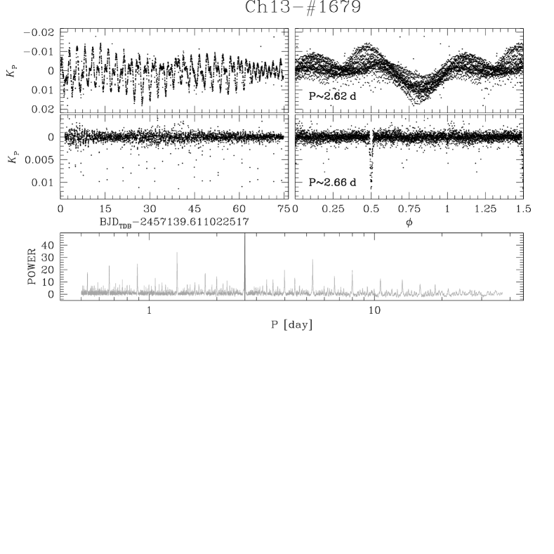
Figure 7: Overview of Ch13-#1679 LC. Top- and middle-left panels show the flattened LCs before and after the flattening and cleaning procedure, respectively. Top- and middle-right panels show the same LCs phased with the periods found with the AoV and BLS periodograms, respectively. Bottom panel shows the BLS normalised periodogram (see text for details).

5.1.2 Star Ch14-#7224

The second object of interest found by our pipeline is star Ch14-#7224 (EPIC 211432103, Fig. 8). Indeed, in K2 this source is a blend of two stars separated by 2.70 arcsec (Heintz 1990). It belongs to the extended input catalogue K2S-Ch14 (see Sect.2.3), derived from the K2 stacked image of Ch14, but we were not able to identify the two components.

While the automatic classification returned a period of P$\sim$0.93 d, a subsequent analysis revealed its nature as EB with period P$\sim$1.86 d, as shown by the different minima of the azure phased LC in the middle-right panel of Fig. 8. Again, the period of the EB is close to that of the activity of the principal component (P$\sim$1.85).

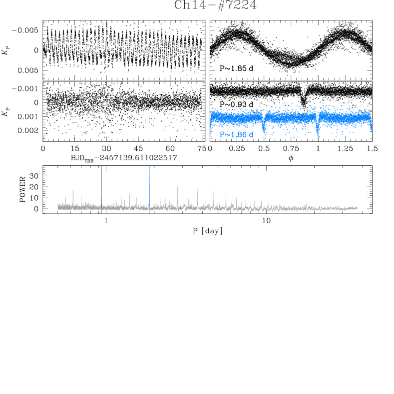
Figure 8: As in Fig. 7, but for star Ch14-#7224 .

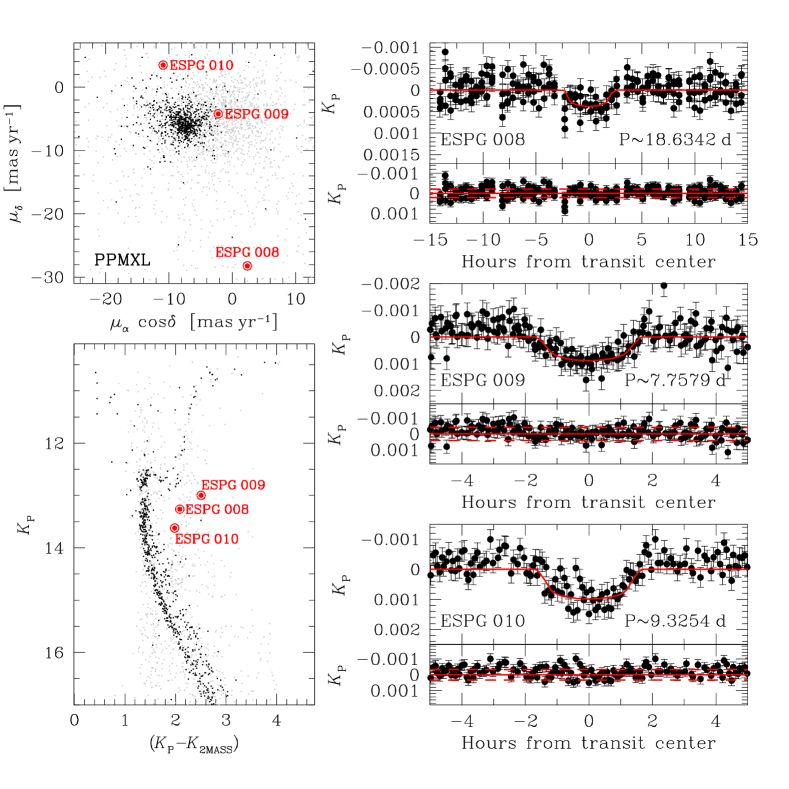
Figure 9: Overview of the three candidate-exoplanets found in this work. Bottom-left panel: $K_{\rm P}$ versus $(K_{\rm P}-K_{\rm 2MASS})$ CMD of M 67; red points mark the location of the three candidate-exoplanet hosts. Top-left panel: PPMXL proper motions for the same stars shown in the bottom-left panel. In both panels, black points are the stars that have a membership probability $\geq 90$% in the Nardiello et al. (2016), in grey the stars that have a lower membership probability in the same catalogue. Right panels: the LCs of the three candidate-exoplanets. For each candidate, on the top, we plot the phased flattened LC (black dots) and the model (red line). The error associated to each point is the 68.27^th percentile of the distribution of the residual from the median value of the LC, excluding transit-points. On the bottom we plot the difference between the observed points and the model. Red solid line is the median of this difference, while dashed red lines correspond to $\pm 1\sigma$.

5.2 Candidate Exoplanets

We found three candidate transiting exoplanets. Firstly, we checked that no other variable star, with similar period, is located close (within 100 Kepler pixels) to each candidate exoplanet.

Transit parameters were obtained using a modified version of the particle-swarm algorithm Pyswarm with the Mandel & Agol (2002) model implemented in PyTransit (Parviainen 2015). In order to compute the corresponding errors, we used the emcee algorithm (Foreman-Mackey et al. 2013). We refer the reader to Paper II for a detailed description of the procedure.

In our transit modelling we fixed the eccentricity $e$ to 0 deg and the argument of pericentre $\omega$ to 90 deg. Exploiting JKTLD code (Southworth 2008), with a quadratic law for limb darkening and the table of Sing (2010), we obtained the linear and quadratic limb darkening parameters for given $T_{\rm eff}$, $\log{g}$, and [M/H] (see next sections), and microturbolence velocity fixed at 2 km s^-1. In the transit modelling, we chose to derive the period ($P$), the mid-transit time of reference ($T_{0}$), the inclination ($i$), and the radii ratio ($R_{\rm P}/R_{\rm S}$).

In the following, we give a brief description of the three candidate-transiting exoplanets and of their parameters found by our analysis. In Fig. 9 we show the position of the three candidates stars on the $K_{\rm P}$ versus $(K_{\rm P}-K_{\rm 2MASS})$ CMD, their proper motions from PPMXL (Roeser et al. 2010), and their phased LCs. Clearly, none of them is a M 67 member.

In Table 1 we list the parameters found of the candidate exoplanets. We emphasise that, as discussed in Paper II, the parameters found by our transit modelling are strongly dependent on the stellar parameters adopted. Because the three stars are not M 67 members, we have to rely on the stellar radii and masses found in the literature, and hence the uncertainties can be large.

5.2.1 ESPG 008

Star Ch13-#6909 (EPIC 211439059, hereafter ESPG 008 following the nomenclature started in Paper II) is not a M 67 member (as demonstrated by its high proper motion in Fig. 9). The depth of the transit is $\sim 310$ ppm.

We adopted the stellar parameters listed in K2 EXOFOP website, provided by Huber et al. (2016).

For this star, EXOFOP gives a stellar radius $R_{\rm S}=(0.821\pm 0.066)\,R_{\odot}$ and a stellar mass $M_{\rm S}=(0.877\pm 0.046)\,M_{\odot}$. Using these stellar values, we found that the hosted candidate-exoplanet has a period of $P\sim 18.6342$ d. We found a radii ratio $R_{\rm P}/R_{\rm S}\sim 0.0166$, corresponding to a planet radius $R_{\rm P}\sim 1.490\,R_{\oplus}$.

This candidate exoplanet was already found by Pope et al. (2016), and the parameters found in this paper are in agreement with what found in their work.

5.2.2 ESPG 009

The candidate exoplanet hosted by the star Ch13-#7099 (EPIC 211390903, S0123, hereafter ESPG 009) is a new detection. The star has a RV$\sim 33.03$ km s^-1 (Geller et al. 2015), in agreement with the mean RV of M 67 ($\sim 33.6$ km s^-1), but from PPMXL proper motions and the CMD, the star seems to be a field star; Sanders (1977) found for this star a membership probability of 38 %.

According to EXOFOP, this star should have a radius $R_{\rm S}=(11.198\pm 0.506)\,R_{\odot}$ and a mass $M_{\rm S}=(1.242\pm 0.132)\,M_{\odot}$, but using these values it is very difficult to fit the transit. We explored the possibility that this star is not a giant, but a K-type main sequence star. We estimated the mass and the radius using different colour indices, the EXOFOP tabulated metallicity (even if the final result is weakly dependent from the [M/H]) and the empirical relations by Boyajian et al. (2012). In this hypothesis we found a $R_{\rm S}=(0.713\pm 0.022)\,R_{\odot}$ and $M_{\rm S}=(0.739\pm 0.020)\,M_{\odot}$. Using these stellar parameters we obtained a better model (lower $\chi^{2}$) than that resulted using EXOFOP parameters. With the assumption that the star is a K-type dwarf, we obtained that the candidate exoplanet has $P\sim 7.7579$ d, $R_{\rm P}/R_{\rm S}\sim 0.0251$, and $R_{\rm P}\sim 1.956\,R_{\oplus}$.

5.2.3 ESPG 010

The LC of the star Ch14-#6981 (EPIC 211413752, hereafter ESPG 010) shows candidate-exoplanet transits of depth $\sim 0.8$ mmag.

For this star EXOFOP gives a stellar radius $R_{\rm S}=(3.666\pm 5.924)\,R_{\odot}$ and a stellar mass $M_{\rm S}=(0.937\pm 0.269)\,M_{\odot}$. Because the error on the stellar radius is large, we decided to calculate the stellar radius and mass as for ESPG 009. We found $R_{\rm S}=(0.713\pm 0.051)\,R_{\odot}$ and $M_{\rm S}=(0.738\pm 0.046)\,M_{\odot}$. From our modelling, we obtained $P\sim 9.3254$ d, $R_{\rm P}/R_{\rm S}\sim 0.0275$, and $R_{\rm P}\sim 2.140\,R_{\oplus}$.

The stellar parameters adopted and the candidate-exoplanet parameters we found are in agreement with the values obtained by Pope et al. (2016).

5.3 Summary on M 67 exoplanets and exoplanets candidates

Brucalassi et al. (2014), using RV measurements, discovered planetary companions around three M 67 members: two main sequence stars (YBP1194 and YBP1514) and an evolved star (SAND364). Another planet hosted by a M 67 MS star (YBP401) was found by Brucalassi et al. (2016). We have verified whether these planets are also transiting, checking their phased LCs with the period found by Brucalassi et al. (2014, 2016) and the periods obtained with our pipeline. None of them showed transit signature.

Pope et al. (2016) released a list of candidate transiting exoplanets in K2/C5 and K2/C6 fields. The two candidate exoplanets found by Pope et al. (2016), located in Ch13 and Ch14, were also found by our pipeline, namely ESPG 008 and ESPG 010 above described.

Recently, Barros et al. (2016) have released a catalogue of candidate-exoplanets from K2/C1 to K2/C6. Two of their candidates fall in our field of view: the first candidate coincides with our ESPG 010; the second one is really the EB Ch14-#7224, described in Sect. 5.1.2.

Table 1: Exoplanet-candidate parameters.

ESPG	EPIC	$\alpha_{\rm J2000}$	$\delta_{\rm J2000}$	$K_{\rm P}$	Period	$T_{0}$	$i$	$R_{\rm P}/R_{\rm S}$	$\delta_{\rm Phot}$	$R_{\rm S}$	$R_{\rm P}$
		(∘)	(∘)		(d)	(KBJD)	(∘)		(%)	($R_{\odot}$)	($R_{\rm Jup}$)
008	211439059	131.97315	12.232101	13.2615	$18.634179\pm 0.005229$	$2350.798089\pm 0.006405$	$89.75\pm 0.10$	$0.0166\pm 0.0005$	$0.031\pm 0.004$	0.821	0.133
009	211390903	132.27813	11.498001	12.9985	$07.757595\pm 0.000822$	$2314.806051\pm 0.003955$	$89.17\pm 0.28$	$0.0251\pm 0.0007$	$0.075\pm 0.006$	0.713	0.174
010	211413752	133.70964	11.848257	13.6226	$09.325429\pm 0.001094$	$2317.180892\pm 0.002211$	$88.71\pm 0.12$	$0.0275\pm 0.0007$	$0.081\pm 0.007$	0.713	0.191

Notes: $\delta_{\rm Phot}$ is calculated as in Paper II.

Table 2: First six lines of Ch13 catalogue.

$\alpha_{\rm J2000}$	$\delta_{\rm J2000}$	$K_{\rm P}$	$B$	$V$	$R$	$I$	$J_{\rm 2MASS}$	$H_{\rm 2MASS}$	$K_{\rm 2MASS}$	ID	$\mu_{\alpha\cos\delta}$	$\mu_{\delta}$	Pμ
(∘)	(∘)										(mas yr-1)	(mas yr-1)	(%)
(1)	(2)	(3)	(4)	(5)	(6)	(7)	(8)	(9)	(10)	(11)	(12)	(13)	(14)
132.96195	11.473325	18.36	20.71	19.19	18.32	17.08	15.61	14.98	14.81	0011	9.0118	-17.0534	09.52
132.74213	11.473428	17.12	18.89	17.70	16.97	16.50	15.11	14.47	14.28	0014	-1.9178	-2.6843	97.33
132.73422	11.475366	15.83	16.99	16.08	15.64	15.47	14.29	13.82	13.76	0020	-2.5016	-2.5507	98.06
132.73256	11.478913	15.69	17.53	16.28	15.61	14.99	13.58	12.93	12.81	0028	5.4254	-18.9655	00.00
132.49665	11.478087	13.20	13.76	13.24	13.07	13.09	12.10	11.86	11.79	0031	4.4767	-2.5405	47.51
132.54849	11.481701	17.10	18.79	17.65	16.92	16.48	15.10	14.54	14.40	0045	-0.0164	-4.7174	88.89

Table 3: First six lines of Ch13 catalogue of variables.

$\alpha_{\rm J2000}$	$\delta_{\rm J2000}$	$P$	$K_{\rm P}$	$B$	$V$	$R$	$I$	$J_{\rm 2MASS}$	$H_{\rm 2MASS}$	$K_{\rm 2MASS}$	ID	Pμ	Blend
(∘)	(∘)	(d)										(%)
(1)	(2)	(3)	(4)	(5)	(6)	(7)	(8)	(9)	(10)	(11)	(12)	(13)	(14)
132.73422	11.475366	14.8451	15.83	16.99	16.08	15.64	15.47	14.29	13.82	13.76	0020	98.06	1
132.78847	11.510606	34.4798	15.94	17.40	16.30	15.80	15.43	14.14	13.58	13.47	0127	98.91	1
132.42671	11.508618	6.6619	11.36	11.88	11.38	11.13	11.47	10.33	10.10	10.05	0128	02.95	1
132.72106	11.522206	5.7137	13.36	14.03	13.44	13.24	13.22	12.25	12.01	11.92	0164	99.13	1
132.38670	11.530417	74.8200	11.38	12.00	11.61	11.12	11.42	10.14	9.80	9.72	0194	93.59	1
132.80516	11.540195	74.8200	17.09	18.93	17.63	17.00	16.46	15.11	14.39	14.19	0208	97.60	1

6 Electronic material

We release raw and detrended LCs of all the sources extracted using aperture and PSF photometric methods.

We also make public the two astro-photometric catalogues of all sources for which we extracted the LCs, one for each analysed channel. The catalogues contain the following information: Cols (1) and (2) are the J2000.0 equatorial coordinates in decimal degrees; Cols (3)-(10) are the calibrated $K_{\rm P}BVRIJ_{\rm 2MASS}H_{\rm 2MASS}K_{\rm 2MASS}$ magnitudes (when the magnitude is not available, it is flagged with $-$99.999); Col. (11) is the identification number of the star; Cols (12) and (13) are the AIC-M67 relative proper motions in mas yr^-1 along $(\alpha\cos\delta,\delta)$ direction (when it is not available, it is flagged with $-$999.9999); Col. (14) is the membership probability (when it is not available, it is flagged with $-1$). Table 2 is an example of the first six rows of the Ch13 catalogue.

We release also two catalogues (one for each analysed channel) containing the variable stars: Cols (1) and (2) are the J2000.0 equatorial coordinates in decimal degrees; Col. (3) is the period found (when the variability is irregular, the period is equal to 74.82); Cols (4)-(11) give the calibrated $K_{\rm P}BVRIJ_{\rm MASS}H_{\rm MASS}K_{\rm MASS}$ magnitudes (when the magnitude is not available, it is flagged with $-$99.999); Col. (12) is the identification number of the star; Col. (13) is the membership probability (when it is not available, it is flagged with $-1$); Col. (14) is a flag that describe our classification of LC: flag=1 high probability to be a real variable star, flag=2 difficult interpretation, flag=3 high probability to be a blend. Table 3 is an example of the first six rows of the Ch13 catalogue of variable stars.

Finally, the publicly available electronic material contains also the two $K2$ astrometrized stacked images (Fig. 1).

7 Summary

In this work we presented K2 LCs extracted from images collected during the K2/C5. We have focused on a region containing the super-stamps that cover the OC M 67 and on all the TPFs in Ch13 and Ch14.

For the LC extraction, we followed the same approach described in Libralato et al. (2016b), based on the use of an high-angular resolution input catalogue, local transformations, effective time-perturbed PSFs and on the subtraction of neighbour stars. Our method is very efficient for extracting LCs of stars located in crowded regions (such as M 67 in K2 images) and for faint stars ($K_{\rm P}>15.5$).

We searched for variable stars among the 4142 extracted LCs, finding a total of 451 variables. Of these objects, 299 are new detection. We found three candidate transiting exoplanets, one of them is a new detection. All the host stars seems to be field stars rather than M 67 members.

We release to the community all raw and detrended LCs. This is the first complete K2 data-set of stellar LCs for the M 67 super-stamp region. We also release the astro-photometric catalogues of all the sources and of the identified variable stars, as well as the astrometrized stacked images.

Our PSF-based approach is suitable for any kind of data, both ground- and space-based observations. The work on K2 data we carried out in this series, is also a benchmark to be ready for the future space missions focused on the search for exoplanets, such as TESS (Transiting Exoplanet Survey Satellite, Ricker et al. 2014) and PLATO (PLAnetary Transits and stellar Oscillations, Rauer et al. 2014) .

References

- Anderson & King (2000) Anderson J., King I. R., 2000, PASP, 112, 1360
- Barros et al. (2016) Barros S. C. C., Demangeon O., Deleuil M., 2016, preprint, (arXiv:1607.02339)
- Bellini et al. (2010) Bellini A., et al., 2010, A&A, 513, A50
- Boyajian et al. (2012) Boyajian T. S., et al., 2012, ApJ, 757, 112
- Brucalassi et al. (2014) Brucalassi A., et al., 2014, A&A, 561, L9
- Brucalassi et al. (2016) Brucalassi A., et al., 2016, A&A, 592, L1
- Bruntt et al. (2007) Bruntt H., et al., 2007, MNRAS, 378, 1371
- Christiansen et al. (2013) Christiansen J. L., Jenkins J., Caldwell D., et al. 2013, Kepler Data Characteristics Handbook
- Foreman-Mackey et al. (2013) Foreman-Mackey D., Hogg D. W., Lang D., Goodman J., 2013, PASP, 125, 306
- Geller et al. (2015) Geller A. M., Latham D. W., Mathieu R. D., 2015, AJ, 150, 97
- Gilliland et al. (1991) Gilliland R. L., et al., 1991, AJ, 101, 541
- Gonzalez (2016) Gonzalez G., 2016, MNRAS,
- Hartman & Bakos (2016) Hartman J. D., Bakos G. Á., 2016, Astronomy and Computing, 17, 1
- Heintz (1990) Heintz W. D., 1990, ApJS, 74, 275
- Heiter et al. (2014) Heiter U., Soubiran C., Netopil M., Paunzen E., 2014, A&A, 561, A93
- Howell et al. (2014) Howell S. B., et al., 2014, PASP, 126, 398
- Huber et al. (2016) Huber D., et al., 2016, ApJS, 224, 2
- Kovács et al. (2002) Kovács G., Zucker S., Mazeh T., 2002, A&A, 391, 369
- Libralato et al. (2016a) Libralato M., et al., 2016a, preprint, (arXiv:1608.00459)
- Libralato et al. (2016b) Libralato M., Bedin L. R., Nardiello D., Piotto G., 2016b, MNRAS, 456, 1137
- Malavolta et al. (2016) Malavolta L., et al., 2016, A&A, 588, A118
- Mandel & Agol (2002) Mandel K., Agol E., 2002, ApJ, 580, L171
- Moré et al. (1980) Moré J. J., Garbow B. S., Hillstrom K. E., 1980, Technical Report ANL-80-74, User guide for MINPACK-1. Argonne Nat. Lab., Argonne, IL
- Nardiello et al. (2015) Nardiello D., et al., 2015, MNRAS, 447, 3536
- Nardiello et al. (2016) Nardiello D., Libralato M., Bedin L. R., Piotto G., Ochner P., Cunial A., Borsato L., Granata V., 2016, MNRAS, 455, 2337
- Pandey et al. (2010) Pandey A. K., Sandhu T. S., Sagar R., Battinelli P., 2010, MNRAS, 403, 1491
- Parviainen (2015) Parviainen H., 2015, MNRAS, 450, 3233
- Pope et al. (2016) Pope B. J. S., Parviainen H., Aigrain S., 2016, preprint, (arXiv:1606.01264)
- Pribulla et al. (2008) Pribulla T., et al., 2008, MNRAS, 391, 343
- Quinn et al. (2012) Quinn S. N., et al., 2012, ApJ, 756, L33
- Quinn et al. (2014) Quinn S. N., et al., 2014, ApJ, 787, 27
- Rauer et al. (2014) Rauer H., et al., 2014, Experimental Astronomy, 38, 249
- Ricker et al. (2014) Ricker G. R., et al., 2014, in Space Telescopes and Instrumentation 2014: Optical, Infrared, and Millimeter Wave. p. 914320 (arXiv:1406.0151), doi:10.1117/12.2063489
- Roeser et al. (2010) Roeser S., Demleitner M., Schilbach E., 2010, AJ, 139, 2440
- Sanders (1977) Sanders W. L., 1977, A&AS, 27, 89
- Sandquist & Shetrone (2003a) Sandquist E. L., Shetrone M. D., 2003a, AJ, 125, 2173
- Sandquist & Shetrone (2003b) Sandquist E. L., Shetrone M. D., 2003b, AJ, 126, 2954
- Schwarzenberg-Czerny (1989) Schwarzenberg-Czerny A., 1989, MNRAS, 241, 153
- Sing (2010) Sing D. K., 2010, A&A, 510, A21
- Southworth (2008) Southworth J., 2008, MNRAS, 386, 1644
- Stassun et al. (2002) Stassun K. G., van den Berg M., Mathieu R. D., Verbunt F., 2002, A&A, 382, 899
- Stello et al. (2006) Stello D., et al., 2006, MNRAS, 373, 1141
- Stello et al. (2007) Stello D., et al., 2007, MNRAS, 377, 584
- Vanderburg & Johnson (2014) Vanderburg A., Johnson J. A., 2014, PASP, 126, 948
- Vanderburg et al. (2016) Vanderburg A., et al., 2016, ApJS, 222, 14
- Yakut et al. (2009) Yakut K., et al., 2009, A&A, 503, 165
- Zechmeister & Kürster (2009) Zechmeister M., Kürster M., 2009, A&A, 496, 577
- van den Berg et al. (2002) van den Berg M., Stassun K. G., Verbunt F., Mathieu R. D., 2002, A&A, 382, 888
- van den Berg et al. (2004) van den Berg M., Tagliaferri G., Belloni T., Verbunt F., 2004, A&A, 418, 509