Parametric Presburger Arithmetic:
Logic, Combinatorics, and
Quasi-polynomial Behavior

Abstract

Parametric Presburger arithmetic concerns families of sets $S_{t}\subseteq{}^{d}$, for $t\in\N$, that are defined using addition, inequalities, constants in , Boolean operations, multiplication by $t$, and quantifiers on variables ranging over . That is, such families are defined using quantifiers and Boolean combinations of formulas of the form $\mathchoice{\mbox{\boldmath$\displaystyle\bf a$}}{\mbox{\boldmath$\textstyle\bf a$}}{\mbox{\boldmath$\scriptstyle\bf a$}}{\mbox{\boldmath$\scriptscriptstyle\bf a$}}(t)\cdot\mathbf{x}\leq b(t),$ where $\mathchoice{\mbox{\boldmath$\displaystyle\bf a$}}{\mbox{\boldmath$\textstyle\bf a$}}{\mbox{\boldmath$\scriptstyle\bf a$}}{\mbox{\boldmath$\scriptscriptstyle\bf a$}}(t)\in\Z[t]^{d},b(t)\in\Z[t]$. A function $g:\N\rightarrow\Z$ is a quasi-polynomial if there exists a period $m$ and polynomials $f_{0},\ldots,f_{m-1}\in\Q[t]$ such that $g(t)=f_{i}(t),\text{ for }t\equiv i\bmod m.$

Recent results of Chen, Li, Sam; Calegari, Walker; Roune, Woods; and Shen concern specific families in parametric Presburger arithmetic that exhibit quasi-polynomial behavior. For example, $\lvert S_{t}\rvert$ might be a quasi-polynomial function of $t$ or an element $\mathbf{x}(t)\in S_{t}$ might be specifiable as a function with quasi-polynomial coordinates, for sufficiently large $t$. Woods conjectured that all parametric Presburger sets exhibit this quasi-polynomial behavior. Here, we prove this conjecture, using various tools from logic and combinatorics.

title = Parametric Presburger Arithmetic: Logic, Combinatorics, and Quasi-polynomial Behavior, author = Tristram Bogart, John Goodrick, and Kevin Woods, plaintextauthor = Tristram Bogart, John Goodrick, and Kevin Woods, keywords = Presburger arithmetic, quasi-polynomials, lattice points, Ehrhart polynomials year=2017, number=4, received=13 September 2016, published=16 January 2017, doi=10.19086/da.1254,

[classification=text]

1 Introduction

We examine a broad class of problems that exhibit quasi-polynomial behavior.

Definition 1.1.

A function $g:\N\rightarrow\Z$ is a quasi-polynomial if there exists a period $m$ and polynomials $f_{0},\ldots,f_{m-1}\in\Q[t]$ such that

$$g(t)=f_{i}(t),\text{ for }t\equiv i\bmod m.$$

A function $g:\N\rightarrow\Z$ is an eventual quasi-polynomial, abbreviated EQP, if it agrees with a quasi-polynomial for sufficiently large $t$. (In this paper, we take $\N=\{0,1,2,\ldots\}$.)

Example 1.2.

$$g(t)=\left\lfloor\frac{t+1}{2}\right\rfloor=\begin{cases}\frac{t}{2}&\text{if $t$ even},\\ \frac{t+1}{2}&\text{if $t$ odd},\end{cases}$$

is a quasi-polynomial with period 2.

In [19], Woods noticed that several recent results concern different kinds of EQP behavior in combinatorially defined families. For example, given a family of sets $S_{t}\subseteq{}^{d}$ for $t\in\N$, $\lvert S_{t}\rvert$ might be an EQP function of $t$ or an element $\mathbf{x}(t)\in S_{t}$ might be specifiable as a function with EQP coordinates. These results are all concerned with the following types of sets [19]:

Definition 1.3.

Given $d\in\N$, a parametric Presburger family is a collection $\{S_{t}:t\in\N\}$ of subsets of ^d which can be defined by a formula using addition, inequalities, multiplication and addition by constants from , Boolean operations (and, or, not), multiplication by $t$, and quantifiers ($\forall$, $\exists$) on variables ranging over . That is, such families are defined using quantifiers and Boolean combinations of formulas of the form $\mathchoice{\mbox{\boldmath$\displaystyle\bf a$}}{\mbox{\boldmath$\textstyle\bf a$}}{\mbox{\boldmath$\scriptstyle\bf a$}}{\mbox{\boldmath$\scriptscriptstyle\bf a$}}(t)\cdot\mathbf{x}\leq b(t),$ where $\mathchoice{\mbox{\boldmath$\displaystyle\bf a$}}{\mbox{\boldmath$\textstyle\bf a$}}{\mbox{\boldmath$\scriptstyle\bf a$}}{\mbox{\boldmath$\scriptscriptstyle\bf a$}}(t)\in\Z[t]^{d},b(t)\in\Z[t]$.

In Section 1.1, we give a number of examples of parametric Presburger families, and discuss their previously known EQP behavior. Note that, for fixed $t$, a formula $\mathchoice{\mbox{\boldmath$\displaystyle\bf a$}}{\mbox{\boldmath$\textstyle\bf a$}}{\mbox{\boldmath$\scriptstyle\bf a$}}{\mbox{\boldmath$\scriptscriptstyle\bf a$}}(t)\cdot\mathbf{x}\leq b(t)$ is simply a linear inequality; as $t$ changes, the half-space that this linear inequality defines both shifts (as $b(t)$ changes) and rotates (as $\mathchoice{\mbox{\boldmath$\displaystyle\bf a$}}{\mbox{\boldmath$\textstyle\bf a$}}{\mbox{\boldmath$\scriptstyle\bf a$}}{\mbox{\boldmath$\scriptscriptstyle\bf a$}}(t)$ changes). It is important to emphasize that we do not allow quantifiers $\exists t$ or $\forall t$ applied to the parameter $t$.

In [19], Woods conjectured that these parametric Presburger families always have EQP behavior. In this paper, we prove this conjecture. After seeing several examples in Section 1.1, we state this theorem precisely in Section 1.2.

1.1 Examples

Example 1.4.

Let $S_{t}$ be the set of integer points, $\mathbf{x}\in{}^{d}$, in a parametric polyhedron defined by a conjunction of linear inequalities of the form $\mathchoice{\mbox{\boldmath$\displaystyle\bf a$}}{\mbox{\boldmath$\textstyle\bf a$}}{\mbox{\boldmath$\scriptstyle\bf a$}}{\mbox{\boldmath$\scriptscriptstyle\bf a$}}\cdot\mathchoice{\mbox{\boldmath$\displaystyle\bf x$}}{\mbox{\boldmath$\textstyle\bf x$}}{\mbox{\boldmath$\scriptstyle\bf x$}}{\mbox{\boldmath$\scriptscriptstyle\bf x$}}\leq tb$, where $\mathchoice{\mbox{\boldmath$\displaystyle\bf a$}}{\mbox{\boldmath$\textstyle\bf a$}}{\mbox{\boldmath$\scriptstyle\bf a$}}{\mbox{\boldmath$\scriptscriptstyle\bf a$}}\in{}^{d}$ and $b\in\Z$. That is, $S_{t}=tP\cap{}^{d}$ for some rational polyhedron $P\subseteq{}^{d}$.

Ehrhart proved [5] that $\lvert S_{t}\rvert$ (if finite) is a quasi-polynomial, with a period given by the smallest $m$ such that $mP$ has integer vertices. This is the classic quasi-polynomial result; see the book [1] by Beck and Robins for a proof and many examples of its utility. As a concrete example:

Example 1.5.

Let $P$ be the triangle with vertices $(0,0)$, $\left(\frac{1}{2},0\right)$, and $\left(\frac{1}{2},\frac{1}{2}\right)$. Then

$$g(t)=\#(tP\cap{}^{2})=\frac{\big{(}\left\lfloor t/2\right\rfloor+1\big{)}\big{(}\left\lfloor t/2\right\rfloor+2\big{)}}{2}=\begin{cases}(t+2)(t+4)/8&\text{if $t$ even,}\\ (t+1)(t+3)/8&\text{if $t$ odd,}\end{cases}$$

is a quasi-polynomial with period 2.

More recently, Chen, Li, and Sam proved [3] that $\lvert S_{t}\rvert$ is still an EQP, even if the normal vectors in the linear inequalities are allowed to vary with $t$, that is, if they are of the form $\mathchoice{\mbox{\boldmath$\displaystyle\bf a$}}{\mbox{\boldmath$\textstyle\bf a$}}{\mbox{\boldmath$\scriptstyle\bf a$}}{\mbox{\boldmath$\scriptscriptstyle\bf a$}}(t)\cdot\mathbf{x}\leq b(t),$ where $\mathchoice{\mbox{\boldmath$\displaystyle\bf a$}}{\mbox{\boldmath$\textstyle\bf a$}}{\mbox{\boldmath$\scriptstyle\bf a$}}{\mbox{\boldmath$\scriptscriptstyle\bf a$}}(t)\in\Z[t]^{d},b(t)\in\Z[t]$.

For a concrete example:

Example 1.6.

Let $P_{t}$ be the “twisting square” in Figure 1a, defined by

$$P_{t}=\big{\{}(x,y)\in\mathbb{R}^{2}:\ \lvert 2x+(2t-2)y\rvert\leq t^{2}-2t+2,\ \lvert(2-2t)x+2y\rvert\leq t^{2}-2t+2\big{\}}.$$

Then $\lvert P_{t}\cap{}^{2}\rvert$ is given by the quasi-polynomial

$$\lvert P_{t}\cap{}^{2}\rvert=\begin{cases}t^{2}-2t+2&\text{if $t$ odd,}\\ t^{2}-2t+5&\text{if $t$ even}.\end{cases}$$

Figure 1: The twisting square $P_{t}$ from Example 1.6.

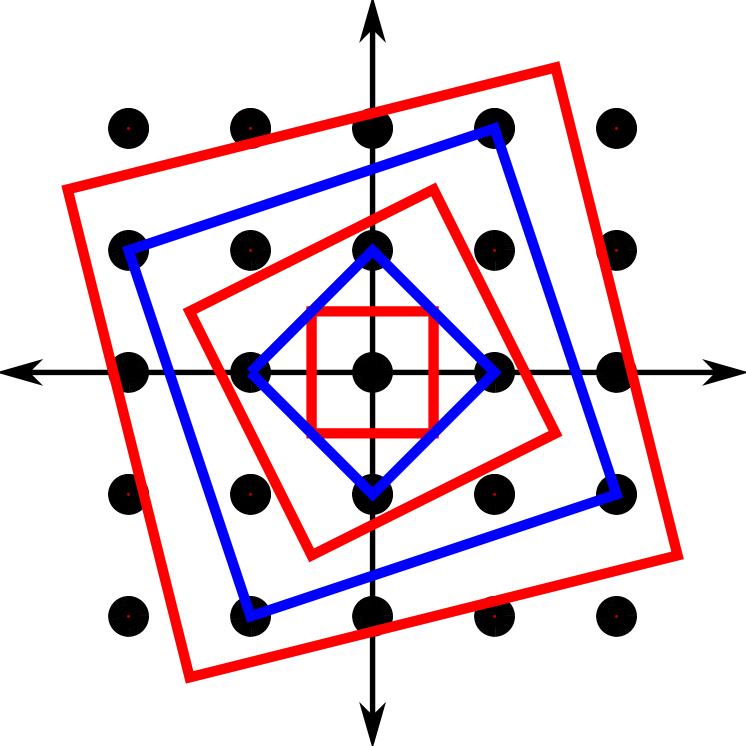
(a) $P_{t}$ for $t=1,\ldots,5$.

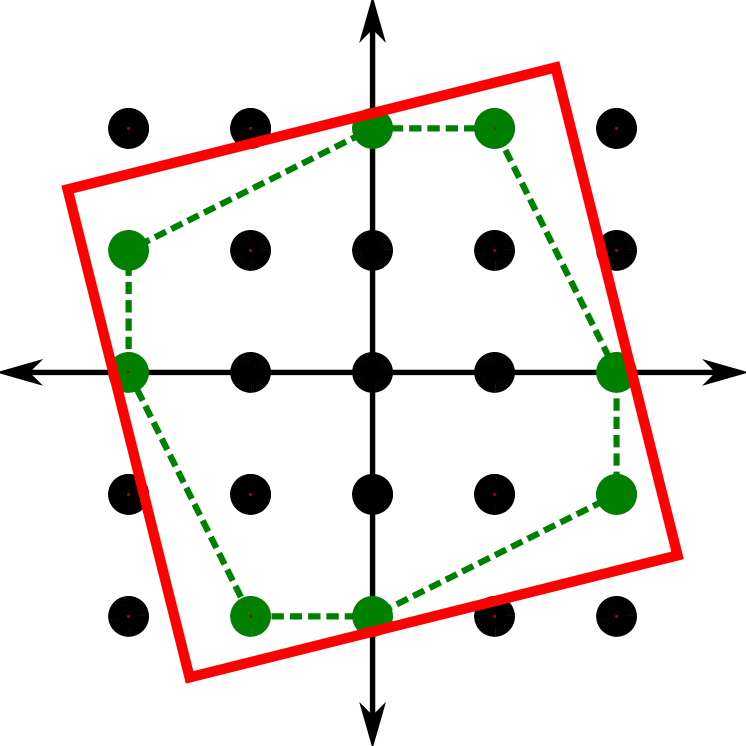
(b) Integer hull of $P_{5}$.

Calegari and Walker were similarly concerned [2] with the integer points in a polyhedron, $P_{t}$, defined by linear inequalities of the form $\mathchoice{\mbox{\boldmath$\displaystyle\bf a$}}{\mbox{\boldmath$\textstyle\bf a$}}{\mbox{\boldmath$\scriptstyle\bf a$}}{\mbox{\boldmath$\scriptscriptstyle\bf a$}}(t)\cdot\mathbf{x}\leq b(t)$. Rather than counting $\lvert P_{t}\cap{}^{d}\rvert$, they wanted to find the vertices of the integer hull of $P_{t}$, that is, the vertices of the convex hull of $P_{t}\cap{}^{d}$.

Example 1.7.

Consider the twisting square, $P_{t}$, from Example 1.6. When $t$ is even, the vertices of $P_{t}$ are integers, so the vertices of the integer hull are simply the vertices of $P_{t}$:

$$\left(\pm\frac{t-2}{2},\pm\frac{t}{2}\right)\quad\text{and}\quad\left(\pm\frac{t}{2},\mp\frac{t-2}{2}\right).$$

When $t$ is odd, the integer hull of $P_{t}$ is an octagon (pictured in Figure 1b for $t=5$) with vertices

$$\left(0,\pm\frac{t-1}{2}\right),\left(\pm\frac{t-3}{2},\pm\frac{t-1}{2}\right),\left(\pm\frac{t-1}{2},0\right),\left(\pm\frac{t-1}{2},\mp\frac{t-3}{2}\right).$$

Abstracting from the last example, the following turns out to be true (first proved by Calegari and Walker [2] under an additional hypothesis on $P_{t}$, later proved in general by Shen [17]):

Theorem 1.8.

Suppose that $P_{t}\subseteq{}^{d}$ is a family of polyhedra defined by a finite conjunction of linear inequalities $\mathchoice{\mbox{\boldmath$\displaystyle\bf a$}}{\mbox{\boldmath$\textstyle\bf a$}}{\mbox{\boldmath$\scriptstyle\bf a$}}{\mbox{\boldmath$\scriptscriptstyle\bf a$}}(t)\cdot\mathbf{x}\leq b(t)$ where $\mathchoice{\mbox{\boldmath$\displaystyle\bf a$}}{\mbox{\boldmath$\textstyle\bf a$}}{\mbox{\boldmath$\scriptstyle\bf a$}}{\mbox{\boldmath$\scriptscriptstyle\bf a$}}\in\Z[t]^{d}$, $b\in\Z[t]$, and that every $P_{t}$ is bounded. Then there exists a modulus $m$ and functions $\mathchoice{\mbox{\boldmath$\displaystyle\bf p$}}{\mbox{\boldmath$\textstyle\bf p$}}{\mbox{\boldmath$\scriptstyle\bf p$}}{\mbox{\boldmath$\scriptscriptstyle\bf p$}}_{ij}:\N\rightarrow{}^{d}$ with polynomial coordinates such that, for $0\leq i<m$ and for sufficiently large $t\equiv i\bmod m$, the set of vertices of the integer hull of $P_{t}\cap{}^{d}$ is $\{\mathchoice{\mbox{\boldmath$\displaystyle\bf p$}}{\mbox{\boldmath$\textstyle\bf p$}}{\mbox{\boldmath$\scriptstyle\bf p$}}{\mbox{\boldmath$\scriptscriptstyle\bf p$}}_{i1}(t),\mathchoice{\mbox{\boldmath$\displaystyle\bf p$}}{\mbox{\boldmath$\textstyle\bf p$}}{\mbox{\boldmath$\scriptstyle\bf p$}}{\mbox{\boldmath$\scriptscriptstyle\bf p$}}_{i2}(t),\ldots,\mathchoice{\mbox{\boldmath$\displaystyle\bf p$}}{\mbox{\boldmath$\textstyle\bf p$}}{\mbox{\boldmath$\scriptstyle\bf p$}}{\mbox{\boldmath$\scriptscriptstyle\bf p$}}_{ik_{i}}(t)\}$.

Another recent EQP result involves the Frobenius number:

Definition 1.9.

Given $a_{1},\ldots,a_{d}\in\N$, let $S$ be the semigroup generated by the $a_{i}$, that is,

$$S=\{a\in\N:\ \exists\lambda_{1},\ldots,\lambda_{d}\in\N,\ a=\lambda_{1}a_{1}+\cdots+\lambda_{d}a_{d}\}.$$

Note the heavy use of quantifiers in this definition, demonstrating that parametric Presburger arithmetic is a natural setting. If the $a_{i}$ are relatively prime, then $S$ contains all sufficiently large integers, and the Frobenius number is defined to be the largest integer not in $S$. This is easily encoded in Presburger arithmetic as the (unique) element $x\in\N$ satisfying

$$x\notin S\wedge\forall y\in\Z\left(y\notin S\rightarrow y\leq x\right).$$

Now we let $a_{i}=a_{i}(t)$ vary with $t$. Roune and Woods proved [14], in a few special cases, that the Frobenius number is an EQP. More recently, Shen [16] proved that this is always true for any eventually positive $a_{i}\in\Z[t]$.

Example 1.10.

Let $a_{1}(t)=t$, $a_{2}(t)=t+1$, and $a_{3}(t)=t+2$. Then the Frobenius number is

$$\left(\left\lfloor\frac{t-2}{2}\right\rfloor+1\right)t-1.$$

This is a running example in [14].

One more example (from [19]) concisely shows the sort of EQP behavior that may appear:

Example 1.11.

Given $t\in\N$, let

$$S_{t}=\big{\{}x\in\N:\ \exists y\in\N,\ 2x+2y+3=5t\text{ and }t<x\leq y\big{\}}.$$

We can compute that

$$S_{t}=\begin{cases}\left\{t+1,t+2,\ldots,\left\lfloor\frac{5t-3}{4}\right\rfloor\right\}&\text{if $t$ odd, $t\geq 3$,}\\ \emptyset&\text{else.}\end{cases}$$

This set has several properties, which we will formalize in Section 1.2:

1. The set of $t$ such that $S_{t}$ is nonempty is $\{3,5,7,\ldots\}$. This set is eventually periodic.

2. The cardinality of $S_{t}$ is

   $$|S_{t}|=\begin{cases}\left\lfloor\frac{5t-3}{4}\right\rfloor-t&\text{if $t$ odd, $t\geq 3$,}\\ 0&\text{else,}\end{cases}$$

   which is eventually a quasi-polynomial of period 4.

3. When $S_{t}$ is nonempty, we can obtain an element of (indeed, the maximum element of) $S_{t}$ with the function $x(t)=\left\lfloor(5t-3)/4\right\rfloor$, and $x(t)$ is eventually a quasi-polynomial.

4. We can compute the generating function

   $$\sum_{s\in S_{t}}x^{s} =\begin{cases}x^{t+1}+x^{t+2}+\cdots+x^{\left\lfloor(5t-3)/4\right\rfloor}&\text{if $t$ odd, $t\geq 3$,}\\ 0&\text{else,}\end{cases}$$

   $$=\begin{cases}\dfrac{x^{t+1}-x^{\left\lfloor(5t-3)/4)\right\rfloor+1}}{1-x}&\text{if $t$ odd, $t\geq 3$,}\\ 0&\text{else.}\end{cases}$$

   We see that, for fixed $t$, this generating function is a rational function. Considering each residue class of $t\bmod 4$ separately, the exponents in the rational function can eventually be written as polynomials in $t$.

Here are two examples that show that our precise definition of parametric Presburger families is important in order to get EQP behavior:

Example 1.12.

The family

$$S_{t}=\{x\in\Z:\exists y\left[y\geq 0\wedge xy=t\right]\}$$

is not a parametric Presburger family, because two variables (neither of which are the parameter, $t$) are multiplied together. Indeed, $\lvert S_{t}\rvert$ is the number of nonnegative divisors of $t$, which is not an EQP function in $t$.

Example 1.13.

The family

$$S_{s,t}=\big{\{}(x,y)\in{}^{2}:\ x\geq 0\wedge y\geq 0\wedge sx+ty=st\big{\}}$$

has two parameters, $s,t\in\N$. $S_{s,t}$ is an interval in ² with endpoints $(t,0)$ and $(0,s)$, and

$$\lvert S_{s,t}\rvert=\gcd(s,t)+1.$$

For a fixed $s$, this is an EQP function of $t$ (and vice versa), but it is not jointly an EQP function in $s$ and $t$.

1.2 Statement of result

In general, let $S_{t}$, for $t\in\N$, be a family of subsets of ^d and consider the following properties that $S_{t}$ might have, cf. Example 1.11.

Property 1

The set of $t$ such that $S_{t}$ is nonempty is eventually periodic.

Property 2

There exists an EQP $g:\N\rightarrow\N$ such that, if $S_{t}$ has finite cardinality, then $g(t)=\lvert S_{t}\rvert$. The set of $t$ such that $S_{t}$ has finite cardinality is eventually periodic.

Property 3

There exists a function $\mathbf{x}:\N\rightarrow{}^{d}$, whose coordinate functions are EQPs, such that, if $S_{t}$ is nonempty, then $\mathbf{x}(t)\in S_{t}$. The set of $t$ such that $S_{t}$ is nonempty is eventually periodic.

Property 4

(Assuming $S_{t}\subseteq{}^{d}$) There exists a period $m$ such that, for sufficiently large $t\equiv i\bmod m$,

$$\sum_{\mathbf{x}\in S_{t}}\mathbf{z}^{\mathbf{x}}=\frac{\sum_{j=1}^{n_{i}}\alpha_{ij}\mathbf{z}^{\mathbf{q_{ij}}(t)}}{(1-\mathbf{z}^{\mathbf{b_{i1}}(t)})\cdots(1-\mathbf{z}^{\mathbf{b_{ik_{i}}}(t)})},$$

where $\alpha_{ij}\in\Q$, and the coordinate functions of $\mathbf{q_{ij}},\mathbf{b_{ij}}:\N\rightarrow{}^{d}$ are polynomials with the $\mathbf{b_{ij}}(t)$ eventually lexicographically positive. (That is, for sufficiently large $t$, the vector $\mathbf{b_{ij}}(t)$ is nonzero and its first nonzero coordinate is positive.)

Property 2 is about counting all solutions and Property 3 is about obtaining specific solutions, and so they seem somewhat different. Generating functions and Property 4 turn out to be the appropriate common generalization. Woods proves [19, Theorem 3.3] a web of implications among these properties; in particular:

Theorem 1.14.

Let $S_{t}$ be any family of subsets of ^d. If $S_{t}$ satisfies Property 4, then it also satisfies Properties 1, 2, and 3.

Woods conjectures [19] that these properties all hold for parametric Presburger families. The contribution of this paper is to prove this conjecture, namely:

Theorem 1.15.

Suppose $S_{t}\subseteq{}^{d}$ is a parametric Presburger family. Then Properties 1, 2, and 3 all hold. Furthermore, if $S_{t}\subseteq{}^{d}$, then Property 4 holds.

In general, quantifiers and Boolean operations allow us to perform many useful operations on sets. For example, if $S_{t}$ is any parametric Presburger set and $\mathchoice{\mbox{\boldmath$\displaystyle\bf c$}}{\mbox{\boldmath$\textstyle\bf c$}}{\mbox{\boldmath$\scriptstyle\bf c$}}{\mbox{\boldmath$\scriptscriptstyle\bf c$}}\in{}^{d}$ is constant, then the set of $\mathchoice{\mbox{\boldmath$\displaystyle\bf x$}}{\mbox{\boldmath$\textstyle\bf x$}}{\mbox{\boldmath$\scriptstyle\bf x$}}{\mbox{\boldmath$\scriptscriptstyle\bf x$}}\in S_{t}$ maximizing $\mathchoice{\mbox{\boldmath$\displaystyle\bf c$}}{\mbox{\boldmath$\textstyle\bf c$}}{\mbox{\boldmath$\scriptstyle\bf c$}}{\mbox{\boldmath$\scriptscriptstyle\bf c$}}\cdot\mathchoice{\mbox{\boldmath$\displaystyle\bf x$}}{\mbox{\boldmath$\textstyle\bf x$}}{\mbox{\boldmath$\scriptstyle\bf x$}}{\mbox{\boldmath$\scriptscriptstyle\bf x$}}$ can be defined using the parametric Presburger formula

$$\mathbf{x}\in S_{t}\quad\wedge\quad\forall y\in{}^{d}\left(\mathbf{y}\in S_{t}\rightarrow\mathchoice{\mbox{\boldmath$\displaystyle\bf c$}}{\mbox{\boldmath$\textstyle\bf c$}}{\mbox{\boldmath$\scriptstyle\bf c$}}{\mbox{\boldmath$\scriptscriptstyle\bf c$}}\cdot\mathbf{y}\leq\mathchoice{\mbox{\boldmath$\displaystyle\bf c$}}{\mbox{\boldmath$\textstyle\bf c$}}{\mbox{\boldmath$\scriptstyle\bf c$}}{\mbox{\boldmath$\scriptscriptstyle\bf c$}}\cdot\mathbf{x}\right).$$

Likewise, if we know that Property 3 holds for all parametric Presburger families, and if $\mathchoice{\mbox{\boldmath$\displaystyle\bf x$}}{\mbox{\boldmath$\textstyle\bf x$}}{\mbox{\boldmath$\scriptstyle\bf x$}}{\mbox{\boldmath$\scriptscriptstyle\bf x$}}:\N\rightarrow{}^{d}$ is a function with EQP coordinates picking out an element of $S_{t}$ whenever this set is nonempty, then we can apply Property 3 again to the new parametric Presburger family $S_{t}\setminus\{\mathchoice{\mbox{\boldmath$\displaystyle\bf x$}}{\mbox{\boldmath$\textstyle\bf x$}}{\mbox{\boldmath$\scriptstyle\bf x$}}{\mbox{\boldmath$\scriptscriptstyle\bf x$}}(t)\}$ to obtain a function $\mathchoice{\mbox{\boldmath$\displaystyle\bf x$}}{\mbox{\boldmath$\textstyle\bf x$}}{\mbox{\boldmath$\scriptstyle\bf x$}}{\mbox{\boldmath$\scriptscriptstyle\bf x$}}_{2}:\N\rightarrow{}^{d}$ such that whenever $|S_{t}|\geq 2$, the pair $(\mathchoice{\mbox{\boldmath$\displaystyle\bf x$}}{\mbox{\boldmath$\textstyle\bf x$}}{\mbox{\boldmath$\scriptstyle\bf x$}}{\mbox{\boldmath$\scriptscriptstyle\bf x$}}(t),\mathchoice{\mbox{\boldmath$\displaystyle\bf x$}}{\mbox{\boldmath$\textstyle\bf x$}}{\mbox{\boldmath$\scriptstyle\bf x$}}{\mbox{\boldmath$\scriptscriptstyle\bf x$}}_{2}(t))$ selects two distinct elements of $S_{t}$.

Arguing as in the previous paragraph, Woods proved [19, Theorem 3.4] that the following would be an immediate corollary to Theorem 1.15:

Corollary 1.16.

Suppose $S_{t}\subseteq{}^{d}$ is a parametric Presburger family. Then $S_{t}$ has the following properties:

Property 3a

Given $\mathchoice{\mbox{\boldmath$\displaystyle\bf c$}}{\mbox{\boldmath$\textstyle\bf c$}}{\mbox{\boldmath$\scriptstyle\bf c$}}{\mbox{\boldmath$\scriptscriptstyle\bf c$}}\in{}^{d}\setminus\{0\}$, there exists a function $\mathchoice{\mbox{\boldmath$\displaystyle\bf x$}}{\mbox{\boldmath$\textstyle\bf x$}}{\mbox{\boldmath$\scriptstyle\bf x$}}{\mbox{\boldmath$\scriptscriptstyle\bf x$}}:\N\rightarrow{}^{d}$ such that, if $\max_{\mathbf{y}\in S_{t}}\mathchoice{\mbox{\boldmath$\displaystyle\bf c$}}{\mbox{\boldmath$\textstyle\bf c$}}{\mbox{\boldmath$\scriptstyle\bf c$}}{\mbox{\boldmath$\scriptscriptstyle\bf c$}}\cdot\mathbf{y}$ exists, then it is attained at $\mathbf{x}(t)\in S_{t}$, and the coordinate functions of $\mathbf{x}$ are EQPs. The set of $t$ such that the maximum exists is eventually periodic.

Property 3b

Fix $k\in\N$. There exist functions $\mathchoice{\mbox{\boldmath$\displaystyle\bf x$}}{\mbox{\boldmath$\textstyle\bf x$}}{\mbox{\boldmath$\scriptstyle\bf x$}}{\mbox{\boldmath$\scriptscriptstyle\bf x$}}_{1},\ldots,\mathchoice{\mbox{\boldmath$\displaystyle\bf x$}}{\mbox{\boldmath$\textstyle\bf x$}}{\mbox{\boldmath$\scriptstyle\bf x$}}{\mbox{\boldmath$\scriptscriptstyle\bf x$}}_{k}:\N\rightarrow{}^{d}$ such that, if $\lvert S_{t}\rvert\geq k$, then $\mathbf{x}_{1}(t),\ldots,\mathbf{x}_{k}(t)$ are distinct elements of $S_{t}$, and the coordinate functions of $\mathbf{x}_{i}$ are EQPs. The set of $t$ such that $\lvert S_{t}\rvert\geq k$ is eventually periodic.

As a further illustration of the power of parametric Presburger arithmetic, note that the ability to maximize a linear functional allows us to run the beyond-and-beneath algorithm (see Grünbaum [8, Section 5.2]) on the integer points in a parametric polyhedron, $P_{t}$, defined by linear inequalities of the form $\mathchoice{\mbox{\boldmath$\displaystyle\bf a$}}{\mbox{\boldmath$\textstyle\bf a$}}{\mbox{\boldmath$\scriptstyle\bf a$}}{\mbox{\boldmath$\scriptscriptstyle\bf a$}}(t)\cdot\mathbf{x}\leq b(t)$. This will iteratively compute vertices of the integer hull, and they will have EQP coordinates. Given the uniform (across $t$) bound on the number of vertices, as proved in [2], this suffices to re-prove Theorem 1.8. All other theorems discussed in Section 1.1 are immediate consequences of Theorem 1.15.

First, in Section 2 we give an outline of the proof of Theorem 1.15, which combines ideas from logic and combinatorics. We set up the logical foundations carefully in Section 3, and then we prove Properties 1, 2, and 3 for Theorem 1.15 in Section 4. This allows us to prove them in the full generality of ^d, but more importantly it shows that the generating function tools are not necessary: we have enough combinatorial information about the sets $S_{t}$ to prove Properties 1, 2 and 3 directly. In Section 5, we discuss generating functions in more detail and prove Property 4.

2 Outline of Proof

We are given a set $S_{t}$ defined in parametric Presburger arithmetic, whose language we will denote $\mathcal{L}_{\textup{EQP}}$. This language allows (repeated) multiplication by $t$, so that the atomic formulas (the basic building blocks) are of the form $\mathchoice{\mbox{\boldmath$\displaystyle\bf a$}}{\mbox{\boldmath$\textstyle\bf a$}}{\mbox{\boldmath$\scriptstyle\bf a$}}{\mbox{\boldmath$\scriptscriptstyle\bf a$}}(t)\cdot\mathbf{x}\leq b(t)$ or $\mathchoice{\mbox{\boldmath$\displaystyle\bf a$}}{\mbox{\boldmath$\textstyle\bf a$}}{\mbox{\boldmath$\scriptstyle\bf a$}}{\mbox{\boldmath$\scriptscriptstyle\bf a$}}(t)\cdot\mathbf{x}=b(t)$, where $\mathchoice{\mbox{\boldmath$\displaystyle\bf a$}}{\mbox{\boldmath$\textstyle\bf a$}}{\mbox{\boldmath$\scriptstyle\bf a$}}{\mbox{\boldmath$\scriptscriptstyle\bf a$}}(t)\in\Z[t]^{d},b(t)\in\Z[t]$. More complicated formulas may be built up using Boolean operations and quantifiers.

By contrast, the language of standard Presburger arithmetic, which we denote $\mathcal{L}_{Pres}$, does not allow multiplication by $t$, so that its atomic formulas are of the form $\mathchoice{\mbox{\boldmath$\displaystyle\bf a$}}{\mbox{\boldmath$\textstyle\bf a$}}{\mbox{\boldmath$\scriptstyle\bf a$}}{\mbox{\boldmath$\scriptscriptstyle\bf a$}}\cdot\mathbf{x}\leq b$ or $\mathchoice{\mbox{\boldmath$\displaystyle\bf a$}}{\mbox{\boldmath$\textstyle\bf a$}}{\mbox{\boldmath$\scriptstyle\bf a$}}{\mbox{\boldmath$\scriptscriptstyle\bf a$}}\cdot x=b$, where $\mathchoice{\mbox{\boldmath$\displaystyle\bf a$}}{\mbox{\boldmath$\textstyle\bf a$}}{\mbox{\boldmath$\scriptstyle\bf a$}}{\mbox{\boldmath$\scriptscriptstyle\bf a$}}\in{}^{d},b\in\Z$. A standard technique to analyze formulas in $\mathcal{L}_{Pres}$ is quantifier elimination: obtain a logically equivalent formula (one defining the same set) that has no quantifiers.

Example 2.1.

The statements

$$\exists y\left[x+y\leq z\ \wedge\ y\geq 3\right]\quad\text{and}\quad x\leq z-3$$

are logically equivalent modulo the theory of Presburger arithmetic; in the second statement, the quantified variable $y$ has been eliminated.

Presburger originally analyzed [12] (see [13] for a translation) these formulas; Cooper [4] uses the following strategy for quantifier elimination:

Eliminate quantified variables one at a time (innermost to outermost). Since $\forall y\ \varphi(\mathbf{x},y)$ is equivalent to $\neg\exists y\,\neg\varphi(\mathbf{x},y)$, we may assume we are eliminating an existential quantifier from a formula of the form $\exists y\ \varphi(\mathbf{x},y)$. Cooper’s strategy is to find a finite set of candidate $y$’s (each written in terms of $\mathbf{x}$) such that: there exists $y$ making $\varphi(\mathbf{x},y)$ true if and only if one of the candidate $y$’s makes $\varphi(\mathbf{x},y)$ true.

Example 2.2.

If there exists a $y\in\Z$ such that

$$x+1\leq y\leq z\ \wedge\ 2y\leq 3z-x$$

then $y=x+1$ must be such a $y$ (this is the smallest integer $y$ satisfying the only lower bound on $y$, and therefore it is the most likely $y$ to also satisfy the upper bounds). Substituting in $y=x+1$ eliminates the quantifier, and we are left with

$$x+1\leq z\ \wedge\ 2(x+1)\leq 3z-x.$$

In general, unfortunately, this does not quite work to guarantee that we may eliminate a quantifier. Instead, we may need to introduce some divisibility conditions:

Example 2.3.

If there exists a $y\in\Z$ such that

$$x+1\leq 2y\leq z\ \wedge\ 2y\leq 3z-x$$

then our candidate for $y$ depends on the parity of $x$: if $x$ is odd, then $y=(x+1)/2$ is our candidate, and if $x$ is even, then $y=(x+2)/2$ is our candidate. Allowing ourselves to use divisibility by 2 in the formula, we eliminate $y$ to get:

$$\big{(}2\big{|}x\ \wedge\ x+2\leq z\ \wedge\ x+2\leq 3z-x\big{)}\ \ \vee\ \ \big{(}2\big{|}(x-1)\ \wedge\ x+1\leq z\ \wedge\ x+1\leq 3z-x\big{)}.$$

To completely eliminate all quantifies in $\mathcal{L}_{Pres}$, we must extend our language to $\mathcal{L}^{+}_{Pres}$, where testing divisibility by a constant, $c$, is allowed. Formally, we introduce divisibility predicates, $D_{c}$, for constants $c$, into our language. For example, we write $2\big{|}(x-1)$ as $D_{2}(x-1)$.

Our proof begins by trying to apply these techniques in $\mathcal{L}_{\textup{EQP}}$, where multiplication by $t$ is allowed.

Step 1: Goodrick does exactly this in [7] (and Lasaruk and Sturm [11] independently arrived at essentially the same result using a different technique). Not surprisingly, we need to extend our language to $\mathcal{L}^{+}_{\textup{EQP}}$, where we are also allowed to test divisibility by polynomials in $t$ (that is, we allow divisibility predicates $D_{f(t)}$, where $f(t)$ is a polynomial in $t$). Even this is not quite enough to eliminate quantifiers:

Example 2.4.

If there exists a $y\in\Z$ such that

$$x+1\leq ty\leq z\ \wedge\ ty\leq 3z-x$$

then our candidate for $y$ depends on $x\bmod t$: if $x\equiv i\bmod t$, for $0\leq i\leq t-1$, then $y=(x+t-i)/t$ is our candidate. Unfortunately, we now have $t$ different candidates for $y$, and we cannot simply list them in a formula. Instead, we must write something like:

$$\exists i\left[0\leq i\leq t-1\ \wedge\ t\big{|}(x-i)\ \wedge\ \big{(}x+t-i\leq z\big{)}\ \wedge\ \big{(}x+t-i\leq 3z-x\big{)}\right]$$

We have replaced the old quantified $y$ with a new quantified $i$, but we have gained something: $i$ is bounded by a polynomial in $t$.

Goodrick proves [7] that any parametric Presburger family $\{S_{t}:t\in\N\}$ is definable by an $\mathcal{L}^{+}_{\textup{EQP}}$-formula with polynomially-bounded quantifiers. Using this result, we now have that every quantified variable $y$ is associated with a condition of the form $0\leq y\leq f(t)$, where $f:\N\rightarrow\Z$ is a polynomial function of $t$.

Step 2: Next, we eliminate all occurrences of the divisibility predicates $D_{f(t)}$. We do this by replacing each variable $x_{i}$ by an expression $g(t)\cdot u_{i}+v_{i}$ where $u_{i}$ and $v_{i}$ are new variables, $g$ is a nonnegative common multiple of all the functions $f_{1},\ldots,f_{n}$ which occur in divisibility predicates $D_{f_{i}}$ in the formula, and with the restriction that $0\leq v_{i}<g(t)$. That is, $u_{i}$ and $v_{i}$ represent the quotient and remainder when $x_{i}$ is divided by $g(t)$.

Example 2.5.

Let

$$S_{t}=\{(x_{1},x_{2})\in{}^{2}:\ D_{t+1}(x_{1}+2x_{2})\ \wedge\ D_{t}(x_{1}-x_{2})\}.$$

Let $g(t)=t(t+1)$ and $x_{i}=g(t)u_{i}+v_{i}$. Then $D_{t+1}(x_{1}+2x_{2})$ is equivalent to $D_{t+1}(v_{1}+2v_{2})$, since $(t+1)\ \big{|}\ g(t)$. Furthermore, $0\leq v_{i}<t(t+1)$ implies that $v_{1}+2v_{2}<3t(t+1)$, and so $D_{t+1}(v_{1}+2v_{2})$ could be replaced by the formula

$$\exists y\left[0\leq y\leq 3t\ \wedge\ y\cdot(t+1)=v_{1}+2v_{2}\right].$$

Replacing both predicates, we define $S^{\prime}_{t}$ as the set

$$\Big{\{}(u_{1},u_{2},v_{1},v_{2}):\ \exists y\left[0\leq y\leq 3t\ \wedge\ y\cdot(t+1)=v_{1}+2v_{2}\right]\wedge\ \exists z\left[-(t+1)\leq z\leq t+1\ \wedge\ z\cdot t=v_{1}-v_{2}\right]\Big{\}}.$$

$S^{\prime}_{t}$ is in bijection to $S_{t}$ under the map $(u_{i},v_{i})\mapsto x_{i}=g(t)u_{i}+v_{i}$.

Notice that we have eliminated the divisibility predicates, at the expense of introducing some additional polynomially-bounded quantifiers. The result of Step 2 is a new parametric Presburger family $S^{\prime}_{t}$ whose points are in bijection with those of $S_{t}$ and such that $S^{\prime}_{t}$ is defined by an $\mathcal{L}_{\textup{EQP}}$-formula with polynomially-bounded quantifiers. Furthermore, the bijection from $S^{\prime}_{t}$ to $S_{t}$ is an affine reduction; that is, it is given by an affine linear function whose coordinates are eventually quasi-polynomial in $t$. We will see that this preserves all the properties of $S_{t}$ that we care about.

Step 3: We now apply a version of Chen–Li–Sam’s “base $t$” method [3], in order to finally eliminate the (polynomially-bounded) quantified variables, $y_{1},\ldots,y_{d}$. After reducing to the case that all variables are nonnegative, suppose that we have some $k$ such that, for all $i$, $0\leq y_{i}<t^{k}$ are bounds on the quantified variables.

We write each $y_{i}$ “base $t$,” using new variables $b_{ij}$:

$$y_{i}=\sum_{j=0}^{k-1}b_{ij}t^{j},\quad 0\leq b_{ij}<t.$$

Suppose that $\ell$ is the largest degree of any polynomial $f(t)$ appearing as a coefficient of some $y_{i}$. Write each free (unquantified) variable, $x_{i}$, in base $t$ using new variables $a_{ij}$ and $z_{i}$:

$$x_{i}=z_{i}t^{k+\ell}+\sum_{j=0}^{k+\ell-1}a_{ij}t^{j},\quad 0\leq a_{ij}<t.$$

Note that we have no bound on the $x_{i}$, so we must allow an unbounded $t^{k+\ell}$ coefficient. The resulting $S^{\prime}_{t}$ will be in bijection with the original $S_{t}$, with the above formulas for $x_{i}$ and $y_{i}$ yielding the bijection. As in Step 2, the bijection is an affine reduction.

We now follow the Chen–Li–Sam method [3], and iteratively look at the $t^{0}$ coefficients of each term, the $t^{1}$ coefficients, etc.

Example 2.6.

Suppose we have the formula

$$0\leq x_{1},x_{2}\wedge\exists y_{1},y_{2}\left[\left(0\leq y_{i}<t^{2}\right)\wedge\left(x_{1}-tx_{2}\leq(t+1)y_{1}+(t+2)y_{2}\right)\right].$$

Replace $y_{i}$ by $b_{i1}t+b_{i0}$ and $x_{i}$ by $z_{i}t^{3}+a_{i2}t^{2}+\cdots+a_{i0}$, with $0\leq b_{ij}<t$ and with $0\leq a_{ij}<t$. That is, $z_{1}$ and $z_{2}$ are the only variables not bounded by $t$. The main inequality is now equivalent to

$$t^{4}(-z_{2})+t^{3}(z_{1}-a_{22})+t^{2}(a_{12}-a_{21}-b_{11}-b_{21})$$

$$+ t(a_{11}-a_{20}-b_{11}-b_{10}-2b_{21}-b_{20})+(a_{10}-b_{10}-2b_{20})\leq 0.$$

Write this inequality as

$$tu+f_{0}\leq 0$$ (1)

where $f_{0}:=a_{10}-b_{10}-2b_{20}$. Since the $a$- and $b$-variables are all bounded between 0 and $t-1$, we see that

$$-3t+3\leq f_{0}\leq t-1.$$

This implies that we are in one of four exclusive cases:

$$\left(-3t+3\leq f_{0}\leq-2t\right)\vee\left(-2t+1\leq f_{0}\leq-t\right)\vee\left(-t+1\leq f_{0}\leq 0\right)\vee\left(1\leq f_{0}\leq t-1\right).$$

Let’s look at the case where $-3t+3\leq f_{0}\leq-2t$ (we will handle each of the finite number of other cases separately.) Dividing inequality (1) by $t$ and taking integer parts, we obtain the equivalent inequality

$$u+\left\lceil\frac{f_{0}}{t}\right\rceil\leq 0.$$

By the hypothesis on $f_{0}$, $\left\lceil\frac{f_{0}}{t}\right\rceil=-2$, so we have reduced to the inequality $u-2\leq 0$, that is,

$$t^{3}(-z_{2}) +t^{2}(z_{1}-a_{22})+t(a_{12}-a_{21}-b_{11}-b_{21})+(a_{11}-a_{20}-b_{11}-b_{10}-2b_{21}-b_{20}-2)\leq 0.$$

Consider the new constant term $f_{1}:=a_{11}-a_{20}-b_{11}-b_{10}-2b_{21}-b_{20}-2$. Again using the bounds on $a_{ij},b_{ij}$ we have

$$-6t+4\leq f_{1}\leq t-3.$$

The relevant seven cases are now

$$\left(-6t+4\leq f_{1}\leq-5t\right)\vee\left(-5t+1\leq f_{1}\leq-4t\right)\vee\cdots\vee\left(1\leq f_{1}\leq t-3\right)$$

and we can again look at them separately. For example, if $-4t+1\leq f_{1}\leq-3t$, then by again dividing by $t$, the original inequality becomes

$$t^{2}(-z_{2})+t(z_{1}-a_{22})+(a_{12}-a_{21}-b_{11}-b_{21}-3)\leq 0.$$

Once again we break into a finite list of cases for the constant term $f_{2}$. For example, in the case

$$-2t+1\leq a_{12}-a_{21}-b_{11}-b_{21}-3\leq-t,$$

the original inequality becomes equivalent to

$$t(-z_{2})+(z_{1}-a_{22}-1)\leq 0.$$ (2)

Since $z_{1}$ is unbounded, we cannot continue with this method. But notice that the case-defining inequalities $-3t+3\leq f_{0}\leq-2t$, $-4t+1\leq f_{1}\leq-3t$, and $-2t+1\leq f_{2}\leq 1$ do not involve multiplication by $t$, and the inequality (2) involves no quantified variables.

This strategy works in general. Our new formula has two types of atomic subformulas: those that involve quantified variables, which are in classical Presburger arithmetic (do not involve multiplication by $t$), and those that use only unquantified variables.

Step 4: We may now apply the classical quantifier elimination procedure to get a logically equivalent quantifier-free formula. Theorem 1.5 from [7] says that this works, because the parameter $t$ does not occur in any of the atomic subformulas involving quantified variables. As discussed before Step 1, we must extend our language to allow $D_{c}$, divisibility predicates for constants $c$. To summarize, we now have a quantifier-free formula in parametric Presburger arithmetic, with the addition of $D_{c}$ predicates.

Step 5: Now that we have a quantifier-free formula, we are ready to understand the geometry of these sets $S_{t}\subseteq{}^{d}$. Our formula consists of atomic formulas of the form

• $\mathbf{f}(t)\cdot\mathbf{x}\leq g(t)$ and

• $D_{c}\big{(}\mathbf{f}(t)\cdot\mathbf{x}-g(t)\big{)}$.

If our formula were simply a conjunction of such atomic formulas, then we would have that

$$S_{t}=P_{t}\cap(\lambda_{t}+\Lambda_{t}),$$

where $P_{t}\subseteq{}^{d}$ is a polyhedron (which changes as $t$ changes) defined by the linear inequalities, $\Lambda_{t}\subseteq{}^{d}$ a lattice, and $\lambda_{t}\in{}^{d}$ a translation vector, with the latter two defined by the divisibility conditions.

Example 2.7.

If $S_{t}$ is the set of $x\in\Z$ such that

$$-x\leq 0\ \wedge\ tx\leq t^{2}+1\ \wedge\ D_{2}(x+t)$$

then

$$P_{t}=[0,(t^{2}+1)/t]\subseteq\R,\quad\Lambda_{t}=2\Z,\quad\lambda_{t}=(t\bmod 2).$$

Of course our $S_{t}$ may not be simply a conjunction of these atomic formulas, so we first show that $S_{t}$ can be written as a disjoint union of such sets, using a variant of Disjunctive Normal Form. Then we may concentrate on each piece individually; $\lvert S_{t}\rvert$, for example, will simply be the sum of the cardinalities of each piece.

So we may assume that $S_{t}$ is a conjunction of these atomic formulas. Note that a conjunction of formulas of the form $D_{c}\big{(}\mathbf{f}(t)\cdot\mathbf{x}-g(t)\big{)}$ is an “external” representation of a translation of a lattice, i.e., defined via constraints, using the language of [15]. We’d like an “internal” representation, i.e., defined parametrically; in this case, this would be a collection of basis vectors for the lattice, together with a translation vector.

Example 2.8.

In Example 2.7, we converted the external representation $D_{2}(x+t)$ into the internal representation: lattice $\Lambda_{t}\subseteq\Z$ with basis $\{2\}$ and translate $\lambda_{t}=(t\bmod 2)$.

By examining Hermite Normal Forms, we prove that this can be accomplished while preserving EQP properties, and then this basis allows us to apply an affine reduction to eliminate any $D_{c}$ terms.

Example 2.9.

Continuing Example 2.7, our internal representation of $\Lambda_{t}+\lambda_{t}$ implies the following: for odd $t$, any $x$ satisfying $D_{2}(x+t)$ is of the form $x=2u+1$, for some $u\in\Z$. Applying the affine reduction given by $x=2u+1$ yields (for odd $t$)

$$S^{\prime}_{t}=\big{\{}u\in\Z:\ -(2u+1)\leq 0\wedge t(2u+1)\leq t^{2}+1\big{\}}.$$

That is, we have eliminated all divisibility terms from the formula.

In other words, we now simply have that $S_{t}$ is the set of integer points in a parametric polyhedron, defined with linear inequalities of the form $\mathbf{f}(t)\cdot\mathbf{x}\leq g(t)$. This is again an “external” representation. We show that we can convert to an “internal” representation and preserve EQP properties, using row reduction over $\Q(t)$. In this case, an internal representation is a list of vertices (given as ratios of EQPs), of extreme rays of the recession cone (encoding directions, $\textstyle\bf y$, in which the polyhedron is infinite in the $\textstyle\bf y$ direction but not in the $-\mathchoice{\mbox{\boldmath$\displaystyle\bf y$}}{\mbox{\boldmath$\textstyle\bf y$}}{\mbox{\boldmath$\scriptstyle\bf y$}}{\mbox{\boldmath$\scriptscriptstyle\bf y$}}$ direction), and of a basis for the lineality space (encoding directions $\textstyle\bf z$ in which it is infinite in both the $\textstyle\bf z$ and $-\mathchoice{\mbox{\boldmath$\displaystyle\bf z$}}{\mbox{\boldmath$\textstyle\bf z$}}{\mbox{\boldmath$\scriptstyle\bf z$}}{\mbox{\boldmath$\scriptscriptstyle\bf z$}}$ directions).

Example 2.10.

Continuing Example 2.7, the external representation $-(2u+1)\leq 0\wedge t(2u+1)\leq t^{2}+1$ defines the polyhedron with vertices $0$ and $(t^{2}-t+1)/2t$. Since this is a bounded polyhedron, the recession cone and the lineality space are trivial.

Step 6: We are now ready to prove Properties 1, 2, and 3. Property 1 will follow from Property 3 trivially. Property 2 follows directly from the Chen, Li, Sam result [3], as long as our polyhedron is bounded. Since we know whether our polyhedron has non-trivial recession cone and lineality space, we know whether it is bounded. If it is unbounded, then $\lvert S_{t}\rvert$ is either 0 or infinite, and we will show how to figure out which is correct. Property 3 similarly follows from Shen [17]. We delay discussion of generating functions until Section 5, but Property 4 follows from Woods [19].

2.1 Summary of Outline of Proof.

Suppose that we are given any parametric Presburger family $S_{t}\subseteq{}^{d}$ defined by an $\mathcal{L}_{\text{EQP}}$-formula $\varphi$. Then we will apply a series of logical equivalences and affine reductions as follows:

$$\varphi\xleftarrow[\text{(Step 1)}]{\text{logic}}\varphi_{1}\xleftarrow[\text{(Step 2)}]{\text{affine}}\varphi_{2}\xleftarrow[\text{(Step 3)}]{\text{affine}}\varphi_{3}\xleftarrow[\text{(Step 4)}]{\text{logic}}\varphi_{4}\xleftarrow[\text{(Step 5)}]{\text{logic + affine}}\varphi_{5}$$

where:

1. $\varphi_{1}$ is an $\mathcal{L}^{+}_{\textup{EQP}}$-formula with polynomially-bounded quantifiers,

2. $\varphi_{2}$ is an $\mathcal{L}_{\textup{EQP}}$-formula with polynomially-bounded quantifiers,

3. $\varphi_{3}$ is an $\mathcal{L}_{\textup{EQP}}$-formula in which no variable within the scope of a quantifier is multiplied by the parameter $t$,

4. $\varphi_{4}$ is a quantifier-free $\mathcal{L}^{+}_{\textup{EQP}}$-formula whose only divisibility predicates are $D_{c}$ for constant functions $c$, and

5. $\varphi_{5}$ is a disjoint union of conjunctions of atomic $\mathcal{L}_{\textup{EQP}}$-formulas (and hence quantifier-free).

At each stage, the reductions preserve all the properties we are interested in, until we finally reduce to the case of the parametric polyhedra defined by $\varphi_{5}$. In Step 6, we deal with these polyhedra by applying previously-established combinatorial techniques from Chen-Li-Sam [3], Woods [19], and Shen [17].

The sequence of reductions is a little complicated, so one might well wonder whether there is a more direct proof. For instance, one might try to show that any $\mathcal{L}_{\text{EQP}}$-formula is logically equivalent to a quantifier-free formula in a slightly larger language with additional “well-behaved” function and relation symbols (the method of quantifier elimination from logic), then prove a generalization of the main theorem from [19] that quantifier-free parametric Presburger formulas have the EQP behavior we seek. But we already know that quantifier elimination in the original language $\mathcal{L}_{\text{EQP}}$ is impossible (see [7]), and finding a reasonable language for quantifier elimination seems difficult. For example, Krajíček [10] gave the name “two-sorted Presburger arithmetic” to the complete first-order theory of as an ordered -module in a language with two sorts of variables (one for the ring, one for the module). Two-sorted Presburger arithmetic is very similar to the logical system studied in this paper, and Krajíček noted “it is an interesting open question whether a form of quantifier elimination holds.” Two-sorted Presburger arithmetic without a relation symbol for $\leq$ was studied by van den Dries and Holly [18], who gave a quantifier elimination theorem for this weaker system in a language including a relation symbol for divisibility and function symbols for gcd and a few other closely related arithmetic functions.

3 Parametric Presburger families and polynomially-bounded quantifiers

In this section, we set notation and definitions and review the result on bounding quantifiers in parametric Presburger families proved in [7]. We also define affine reductions and note that they preserve Properties 1 through 3.

3.1 Parametric Presburger arithmetic

We will use standard notation and terminology from first-order logic, for which any modern textbook on the subject could serve as a reference (for instance, [6] or [9]). In particular, a language is a set of finitary relational, functional, and constant symbols, usually denoted by $\mathcal{L}$ with decorations. Given a language $\mathcal{L}$, an $\mathcal{L}$-formula means a first-order formula in $\mathcal{L}$: we allow basic symbols in $\mathcal{L}$ plus equality, symbols for variables, Boolean operations, and quantifiers.

We let $\mathcal{L}_{Pres}$ be the first-order language with symbols for $0$ and $1$ (constants), $<$ (binary relation for the ordering), $-$ (a unary operation symbol for negation), and $+$ (binary function symbol for addition).

We will always work in the standard model of Presburger arithmetic with universe , so whenever we write “$\models\varphi$” or “$\varphi$ holds” we are referring to the standard interpretation of the language.

$\mathcal{L}^{+}_{Pres}\supseteq\mathcal{L}_{Pres}$ is the expansion which includes unary predicates $D_{c}$ for each $c\in\Z$, to be interpreted as divisibility by $c$. By convention, if $c=0$, then “$D_{0}(x)$” is false for every $x\in\Z$, even if $x=0$.

Now we come to the main definition:

Definition 3.1.

A parametric Presburger formula is a first-order formula in the language $\mathcal{L}_{\textup{EQP}}:=\mathcal{L}_{Pres}\cup\{\lambda_{t}\}$. The intended interpretation of $\lambda_{t}(x)$ is that we are multiplying $x$ by the parameter $t$ which takes some value from .

Given $t\in\N$ and an $\mathcal{L}_{\textup{{EQP}}}$-formula $\varphi$, we define the $\mathcal{L}_{Pres}$-formula $\varphi_{t}$ to be the translation of $\varphi$ defined recursively so that each term of the form $\lambda_{t}(s)$ occurring in $\varphi$ (where $s$ is a term) is replaced by one of the following:

1. If $t>0$, then $\lambda_{t}(s)$ is replaced in $\varphi_{t}$ by $s+s+\ldots+s$ with $t$ repetitions of $s$;

2. if $t=0$, then $\lambda_{t}(s)$ is replaced in $\varphi_{t}$ by the constant symbol $0$.

Remark 3.2.

Here and below, we will adopt the notational convention of writing “$f(t)\cdot s$” for the $\mathcal{L}_{\textup{EQP}}$-term formed from the term $s$ and $f(t)\in\Z[t]$ by repeated applications of the function $\lambda_{t}$. For instance, the expression $(t^{2}+2)\cdot x_{1}$ stands for the term $\lambda_{t}(\lambda_{t}(x_{1}))+x_{1}+x_{1}$.

When we write $\varphi(\mathbf{x})$, we mean that all of the free variables occurring in $\varphi$ are listed in the tuple $\mathbf{x}=(x_{1},\ldots,x_{d})$. (Throughout, boldface letters such as $\mathbf{a}$ and $\mathbf{x}$ will always denote finite tuples.)

The definition of $\varphi_{t}$ above allows us to talk about the truth of $\mathcal{L}_{\textup{EQP}}$-formulas relative to a parameter $t\in\N$: given an $\mathcal{L}_{\textup{EQP}}$-formula $\varphi(x_{1},\ldots,x_{d})$ whose free variables are contained in $\{x_{1},\ldots,x_{d}\}$ and $(k_{1},\ldots,k_{d})\in{}^{d}$, we will write

$$\models\varphi_{t}(k_{1},\ldots,k_{d})$$

just in case the $\mathcal{L}_{Pres}$-formula $\varphi_{t}$ is true with the variable $x_{i}$ evaluated as $k_{i}$.

Definition 3.3.

A parametric Presburger family is a family of sets $\{S_{t}:t\in\N\}$ such that

$$S_{t}=\{(k_{1},\ldots,k_{d})\in{}^{d}:\,\,\,\models\varphi_{t}(k_{1},\ldots,k_{d})\}$$

for some fixed $d$ and some $\mathcal{L}_{\textup{EQP}}$-formula $\varphi(x_{1},\ldots,x_{d})$.

From a logical standpoint, the idea behind parametric Presburger definability is that we are essentially expanding classical Presburger arithmetic by a restricted multiplication function: we allow multiplication of any variable or term by the special parameter variable $t$, but we do not allow multiplication between any of the other variables, and we do not allow quantification over $t$, thus avoiding the complications of sets definable in the full first-order theory of $(\Z;<,+,\cdot)$.

Definition 3.4.

$\mathcal{L}^{+}_{\textup{EQP}}:=\mathcal{L}_{\textup{EQP}}\cup\{D_{f(t)}:f(t)\in\Z[t]\}$, where $D_{f(t)}$ is a unary relation symbol denoting divisibility by the value of $f(t)$.

Given an $\mathcal{L}^{+}_{\textup{EQP}}$-formula $\varphi(x_{1},\ldots,x_{d})$, for any $t\in\N$ and $a_{1},\ldots,a_{d}\in\Z$, we can define the truth value of $\varphi_{t}(a_{1},\ldots,a_{d})$ as before, recalling the convention that $D_{0}(x)$ is always false.

Definition 3.5.

Two $\mathcal{L}^{+}_{\textup{EQP}}$-formulas $\varphi(x_{1},\ldots,x_{d})$ and $\psi(x_{1},\ldots,x_{d})$ are logically equivalent just in case for every $t\in\N$, the $\mathcal{L}^{+}_{Pres}$-formulas $\varphi_{t}$ and $\psi_{t}$ are logically equivalent; in other words, for every $t\in\N$ and every $(k_{1},\ldots,k_{d})\in{}^{d}$,

$$\models\varphi_{t}(k_{1},\ldots,k_{d})\Leftrightarrow\models\psi_{t}(k_{1},\ldots,k_{d}).$$

It is clear that every $\mathcal{L}^{+}_{\textup{EQP}}$-formula is logically equivalent to some $\mathcal{L}_{\textup{EQP}}$-formula.

Definition 3.6.

Given an $\mathcal{L}^{+}_{\textup{EQP}}$-formula $\varphi(x_{1},\ldots,x_{d},y)$ whose free variables are among $\{x_{1},\ldots,x_{d},y\}$ and $f\in\Z[t]$, a polynomially-bounded universal quantifier applied to $\varphi$ yields

$$\forall y\left[0\leq y\leq f(t)\rightarrow\varphi(x_{1},\ldots,x_{d},y)\right]$$

for some $f\in\Z[t]$. Similarly, a polynomially-bounded existential quantifier applied to $\varphi$ yields

$$\exists y\left[0\leq y\leq f(t)\ \wedge\ \varphi(x_{1},\ldots,x_{d},y)\right].$$

An $\mathcal{L}^{+}_{\textup{EQP}}$-formula with polynomially-bounded quantifiers is a member of the smallest class of $\mathcal{L}^{+}_{\textup{EQP}}$-formulas containing all atomic formulas and closed under Boolean combinations and the formation of polynomially-bounded quantifiers.

We recall the following theorem, which was proved in [7]:

Theorem 3.7.

Every $\mathcal{L}^{+}_{\textup{EQP}}$-formula is logically equivalent to an $\mathcal{L}^{+}_{\textup{EQP}}$-formula with polynomially-bounded quantifiers.

Also see [7] for a discussion on how this relates to similar previously-known results of Weispfenning and Lasaruk-Sturm [11].

Assumption 3.8.

In any first-order formula $\varphi$, we always assume that no variable occurs in $\varphi$ both as a free variable and as a quantified variable: that is, formulas such as

$$(x>0)\wedge(y>0)\wedge\exists x\left[x+x=y\right]$$

are not allowed (we have to rename the quantified variable and replace the last conjunct by “$\exists z\left[z+z=y\right]$”).

3.2 Eventual quasi-polynomials and affine reductions

Recall that EQPs were defined in Definition 1.1.

Definition 3.9.

Given any $d^{\prime}\times d$ matrix $A(t)=(f_{i,j}(t))$ of EQP functions and any $d^{\prime}$-tuple $(g_{1}(t),\ldots,g_{d^{\prime}}(t))$ of EQP functions, we call the function $F:{}^{d}\times\N\rightarrow{}^{d^{\prime}}$ given by the rule

$$F(x_{1},\ldots,x_{d},t)=A(t)\cdot(x_{1},\ldots,x_{d})^{T}+(g_{1}(t),\ldots,g_{d^{\prime}}(t))^{T}$$

an EQP-affine function.

Definition 3.10.

Suppose that $S_{t}\subseteq{}^{d}$ and $S^{\prime}_{t}\subseteq{}^{d^{\prime}}$ are parametric Presburger families, defined by $\mathcal{L}^{+}_{\textup{EQP}}$-formulas $\varphi(\mathbf{x})$ and $\varphi^{\prime}(\mathbf{z})$ respectively. We say that $S^{\prime}_{t}$ is affine reducible to $S_{t}$ if there is an EQP-affine function $F:{}^{d^{\prime}}\times\N\rightarrow{}^{d}$ such that for every $t\in\Z$, if $F_{t}$ is the function obtained from $F$ by fixing the value of $t$ for the $(d^{\prime}+1)$-th coordinate, then $F_{t}\upharpoonright S^{\prime}_{t}$ is a bijection from $S^{\prime}_{t}$ onto $S_{t}$.

Abusing notation, we will not always distinguish carefully between an $\mathcal{L}^{+}_{\textup{EQP}}$-definable family and the parametric Presburger set that it defines, and we may say “$\varphi^{\prime}$ is affine reducible to $\varphi$” with the obvious meaning.

The key property of affine reductions for our approach is that they preserve Properties 1, 2, and 3:

Remark 3.11.

If $S_{t}\subseteq{}^{d}$ and $S^{\prime}_{t}\subseteq{}^{d^{\prime}}$ are families parametrized by $t\in\N$ and $S^{\prime}_{t}$ is affine reducible to $S_{t}$, then if $S^{\prime}_{t}$ has any of the Properties 1, 2, or 3, then $S_{t}$ has the same Properties.

Proof.

The preservation of Properties 1 and 2 is trivial, since $F$ induces bijections from the sets $S^{\prime}_{t}$ onto the $S_{t}$. For Property 3, if $F:{}^{d^{\prime}}\times\N\rightarrow{}^{d}$ gives an affine reduction from $S^{\prime}_{t}$ to $S_{t}$ and $\mathchoice{\mbox{\boldmath$\displaystyle\bf x$}}{\mbox{\boldmath$\textstyle\bf x$}}{\mbox{\boldmath$\scriptstyle\bf x$}}{\mbox{\boldmath$\scriptscriptstyle\bf x$}}:\N\rightarrow{}^{d^{\prime}}$ is an EQP-affine function such that $\mathchoice{\mbox{\boldmath$\displaystyle\bf x$}}{\mbox{\boldmath$\textstyle\bf x$}}{\mbox{\boldmath$\scriptstyle\bf x$}}{\mbox{\boldmath$\scriptscriptstyle\bf x$}}(t)\in S^{\prime}_{t}$ (whenever $S^{\prime}_{t}\neq\emptyset$), then the composition $F\circ\mathchoice{\mbox{\boldmath$\displaystyle\bf x$}}{\mbox{\boldmath$\textstyle\bf x$}}{\mbox{\boldmath$\scriptstyle\bf x$}}{\mbox{\boldmath$\scriptscriptstyle\bf x$}}:\N\rightarrow{}^{d}$ is an EQP function yielding points in $S_{t}$ whenever this is nonempty. ∎

4 A sequence of reductions

In this section we give the details of the six steps of our procedure as outlined in Section 2. This will prove Properties 1, 2, and 3 in Theorem 1.15.

4.1 Step 1

This is the content of Theorem 3.7, proved in [7].

4.2 Step 2

Next we describe an affine reduction which eliminates the divisibility predicates $D_{f(t)}$ from an $\mathcal{L}^{+}_{\textup{EQP}}$ formula, but at the cost of adding additional bounded quantifiers and new variables, cf. Example 2.5:

Lemma 4.1.

Let $S_{t}\subseteq{}^{d}$ be a parametric Presburger family defined by an $\mathcal{L}^{+}_{\textup{EQP}}$-formula with polynomially-bounded quantifiers. Then there is a parametric Presburger family $S^{\prime}_{t}\subseteq{}^{d^{\prime}}$ which is definable by an $\mathcal{L}_{EQP}$-formula with polynomially-bounded quantifiers and such that $S^{\prime}_{t}$ is affine reducible to $S_{t}$.

Proof.

Fix some $\mathcal{L}^{+}_{\textup{EQP}}$ formula $\varphi(\mathbf{x})$ with polynomially-bounded quantification which defines the family $S_{t}$. Let $f_{1},\ldots,f_{r}$ be all the functions in $\Z[t]$ which occur in divisibility predicates $D_{f_{i}(t)}$ in $\varphi$. Without loss of generality, none of the $f_{i}$’s is the zero polynomial (since formulas $D_{0}(s)$ are trivially false), so $f_{i}(t)$ is nonzero for sufficiently large $t$. Since $D_{f}$ and $D_{-f}$ are logically equivalent, we may assume that $f_{i}(t)$ is eventually positive. Let $g\in\Z[t]$ be the product $f_{1}f_{2}\cdots f_{r}$. Then for sufficiently large $t\in\N$, the value $g(t)$ is a positive common multiple of $f_{1}(t),\ldots,f_{r}(t)$; there are only finitely many values of $t$ at which one of $f_{1}(t),\ldots,f_{r}(t)$ is nonpositive, and an EQP-affine reduction can handle these cases separately.

Let $z_{1},\ldots,z_{m}$ list all variables occurring in $\varphi$, both free and quantified. Let $u_{1},\ldots,u_{m}$ and $v_{1},\ldots,v_{m}$ be a set of new variables. Let $F:{}^{2m}\times\N\rightarrow{}^{m}$ be the EQP-affine function

$$F(u_{1},\ldots,u_{m},v_{1},\ldots,v_{m},t)=(g(t)\cdot u_{1}+v_{1},\ldots,g(t)\cdot u_{m}+v_{m}).$$

We will now define a formula $\varphi^{\prime}$ whose free variables are among $u_{1},\ldots,u_{m},$ $v_{1},\ldots,v_{m}$ and show that this is affine reducible to $\varphi$ “via $F$”: this means that the restriction of $F$ to the set defined by $\varphi^{\prime}$, ignoring any $u_{i}$ or $v_{i}$ which does not occur free, yields a bijection onto the set $S_{t}$ defined by $\varphi$.

In fact, we will recursively construct $\mathcal{L}_{\textup{EQP}}$-formulas $\psi^{\prime}$ for every subformula $\psi$ of $\varphi$, starting with the atomic subformulas, such that every $\psi^{\prime}$ has polynomially-bounded quantification and the parametric Presburger family defined by $\psi$ is affine reducible to that defined by $\psi^{\prime}$ via the map $F$, and the family $S^{\prime}_{t}$ that we seek will be that defined by $\varphi^{\prime}$.

The formula $\psi^{\prime}$ will be defined as $\theta\wedge\psi^{\prime\prime}$ where $\theta$ is the conjunction

$$\bigwedge_{i=1}^{m}\left[0\leq v_{i}<g(t)\right]$$

and the formula $\psi^{\prime\prime}$ is defined by recursion. As we define the formula $\psi^{\prime\prime}$, we will also show inductively that the following holds:

$(*)$ For any sequence of values $(\mathbf{a},\mathbf{b})=(a_{1},\ldots,a_{m},b_{1},\ldots,b_{m})$ which satisfies $\theta$, we have $\models(\psi^{\prime\prime})_{t}(\mathbf{a},\mathbf{b})$ if and only if $\models\psi_{t}(F(\mathbf{a},\mathbf{b},t))$.

Note that $(*)$ immediately implies that $\psi^{\prime}$ is affine reducible to $\psi$ via $F$.

$\bullet$ For any term $s$ in the variables $z_{1},\ldots,z_{m}$, let $s(g\cdot\mathbf{u}+\mathbf{v}/\mathbf{z})$ be the result of replacing each instance of the variable $z_{i}$ by $g\cdot u_{i}+v_{i}$. Then if $\psi$ is an atomic formula of the form $s_{1}=s_{2}$, we let $\psi^{\prime\prime}$ be the atomic formula

$$s_{1}(g\cdot\mathbf{u}+\mathbf{v}/\mathbf{z})=s_{2}(g\cdot\mathbf{u}+\mathbf{v}/\mathbf{z}).$$

If $\psi$ is an atomic formula of the form $s_{1}\leq s_{2}$, then $\psi^{\prime\prime}$ is

$$s_{1}(g\cdot\mathbf{u}+\mathbf{v}/\mathbf{z})\leq s_{2}(g\cdot\mathbf{u}+\mathbf{v}/\mathbf{z}).$$

It is clear that in this case that $(*)$ holds.

$\bullet$ For any atomic formula $\psi$ of the form $D_{f_{j}(t)}(s)$ (where $s$ is a term), let $h_{s}(t)\in\Z[t]$ be such that $\lvert s^{t}(a_{1},\ldots,a_{m})\rvert\leq h_{s}(t)$, for all $t\in\N$ and all $a_{1},\ldots,a_{m}$ with $0\leq a_{i}<g(t)$ (since, for fixed $t$, $s$ is linear in $a_{1},\ldots,a_{m}$, we only need check the bound on the finite set of $2^{d}$ EQPs obtained by setting each $a_{i}$ to $0$ or to $g(t)$, in the term $s(a_{1},\ldots,a_{m})$). Let $s(\mathbf{v}/\mathbf{z})$ be the result of replacing each instance of each variable $z_{i}$ by $v_{i}$. Now let $\psi^{\prime\prime}$ be the formula

$$\exists y\left[0\leq y\leq h_{s}(t)\ \wedge\ \big{(}f_{j}(t)\cdot y=s(\mathbf{v}/\mathbf{z})\ \vee\ f_{j}(t)\cdot(-y)=s(\mathbf{v}/\mathbf{z})\big{)}\right],$$

where $y$ is a new variable. Note that $\psi^{\prime\prime}$ has polynomially-bounded quantification. The hypothesis $(*)$ asserts that checking that the term $s$ applied to the $g(t)\cdot u_{i}+v_{i}$ is divisible by $f_{j}(t)$ is equivalent to checking the divisibility of $s$ applied to the $v_{i}$: this is true because $g(t)$ is divisible by $f_{j}(t)$.

$\bullet$ $(\psi_{1}\wedge\psi_{2})^{\prime\prime}=\psi_{1}^{\prime\prime}\wedge\psi_{2}^{\prime\prime}$, $(\neg\psi)^{\prime\prime}=\neg(\psi^{\prime\prime})$, $(\psi_{1}\vee\psi_{2})^{\prime\prime}=\psi_{1}^{\prime\prime}\vee\psi_{2}^{\prime\prime}$, and $(\psi_{1}\rightarrow\psi_{2})^{\prime\prime}=\psi_{1}^{\prime\prime}\rightarrow\psi_{2}^{\prime\prime}$. It is routine to check that if $(*)$ holds for the formulas $\psi_{i}$ and $\psi^{\prime\prime}_{i}$, then they continue to hold for the Boolean combinations above. Furthermore, if the formulas $\psi_{i}^{\prime\prime}$ have bounded quantification, then so do all of these Boolean combinations.

$\bullet$ If $\psi$ is a formula of the form $\exists z_{i}\left[0\leq z_{i}\leq h(t)\wedge\theta\right]$ (with polynomially-bounded quantification on the outside), then we define $\psi^{\prime\prime}$ as

$$\exists u_{i}[0\leq u_{i}\leq h(t)\ \wedge$$

$$\exists v_{i}\left[\left(0\leq v_{i}<g(t)\right)\wedge\left(0\leq g(t)\cdot u_{i}+v_{i}\leq h(t)\right)\wedge\theta^{\prime\prime}(g(t)\cdot u_{i}+v_{i}/z_{i})\right]],$$

where “$\theta^{\prime\prime}(g\cdot u_{i}+v_{i}/z_{i})$” means the result of substituting each instance of the free variable $z_{i}$ in the formula $\theta$ with the term $g\cdot u_{i}+v_{i}$. Again, the new formula $\psi^{\prime\prime}$ has polynomially-bounded quantification under the inductive hypothesis that $\theta^{\prime\prime}$ does, and $(*)$ is also immediate by induction. ∎

Remark 4.2.

We note in passing that the same argument can be applied to $\mathcal{L}_{R}$-definable families (in the language of [7]) for any ring $R$ of -valued functions, with only minor modifications. This gives us the following: for any $R$-parametric Presburger family $S_{t}\subseteq{}^{d}$, there is an $R$-parametric Presburger family $S^{\prime}_{t}\subseteq{}^{d^{\prime}}$ which is definable by an $\mathcal{L}_{R}$-formula with $R$-bounded quantifiers and such that $S^{\prime}_{t}$ is $R$-affine reducible to $S_{t}$.

4.3 Step 3

This next step involves writing the variables of our formula in “base $t$,” cf. Example 2.6. To do this, it is most convenient to show that we can reduce to the case where the free variables are nonnegative (by Definition 3.6 for polynomially-bounded quantifiers, the quantified variables are already nonnegative). Indeed, if our free variables are among $(x_{1},\ldots,x_{d})$, we partition ^d into $2^{d}$ pairwise disjoint regions $X_{1},\ldots,X_{2^{d}}$ according whether each free variable $x_{i}$ is negative or nonnegative. Now let $S^{k}_{t}:=X_{k}\cap S_{t}$ for each $k\in\{1,\ldots,2^{d}\}$, and note that $S^{k}_{t}$ is a parametric Presburger family which is EQP-affine reducible to a parametric Presburger family living in ^d (by inverting the values of negative coordinates). Then $S_{t}$ is the disjoint union of these $S^{k}_{t}$, and the following remark shows that we may examine each $S^{k}_{t}$ separately.

Remark 4.3.

If we can write $S_{t}$ as a union $S^{1}_{t}\cup\cdots\cup S^{k}_{t}$ of pairwise disjoint parametric Presburger families, then to prove that $S_{t}$ satisfies Properties 1, 2, and 3 (as in Theorem 1.15), it is sufficient to prove these for each $S^{i}_{t}$ separately. In particular, Property 1 follows because the union of eventually periodic sets is eventually periodic, Property 2 follows because the sum of EQP’s is an EQP, and Property 3 follows because we may specify an $\mathbf{x}(t)$ from any of the (nonempty) sets in the disjoint union.

The following is the main Proposition encompassing Step 3:

Proposition 4.4.

Let $S_{t}\subseteq{}^{d}$ be a parametric Presburger family which is definable by an $\mathcal{L}_{\textup{EQP}}$-formula with polynomially-bounded variables $y_{1},\ldots,y_{m}$. Then there is an EQP-parametric Presburger family $S^{\prime}_{t}$ that is EQP-affine reducible to $S_{t}$ and such that $S^{\prime}_{t}$ is definable by a $\mathcal{L}_{\textup{EQP}}$-formula $\varphi(\mathbf{a},\mathbf{z})$ whose free variables are among the variables $\mathbf{a}$ and $\mathbf{z}$ and whose quantified variables are listed in the finite tuple $\mathbf{b}$ (which is assumed to be disjoint from $\mathbf{a}$ and $\mathbf{z}$), and satisfying the following conditions:

1. The atomic subformulas of $\varphi$ are all of one of two types:

   1. Type 1, which are inequalities involving only variables in $\mathbf{a}$, $\mathbf{b}$, and $t$, and which do not involve any multiplication by $t$;

   2. Type 2, which are inequalities involving only $t$ and the free variables (from $\mathbf{a}$ or from $\mathbf{z}$);

2. Any free variable from $\mathbf{a}$ is explicitly bounded between $0$ and $t-1$ (inclusive) by an atomic subformula of $\varphi$ which is outside the scope of any quantifier or disjunction; and

3. Any quantified variable from $\mathbf{b}$ is bounded between $0$ and $t-1$ (inclusive).

In order to prove Proposition 4.4, we adapt the approach of Chen, Li, and Sam in [3] of writing each variable “base $t$.” We cannot directly apply their results because of the interaction between the potential unboundedness of the free variables and the existence of (bounded) quantified variables. Specifically, their key Lemma 3.2 uses sets defined only by equalities and nonnegativity constraints. We need to work with general linear inequalities and cannot apply the usual procedure of introducing slack variables to convert them into equalities because of the presence of quantifiers.

For example, consider the set $S$ given by

$$S=\{x\in\Z:x\geq 0\wedge\exists y\left[(y\geq 0)\wedge(x+y\leq 2)\right]\}\;=\;\{0,1,2\}.$$

Since $x$ and $y$ are nonnegative, we could introduce a slack variable $w$ to obtain the set $S^{\prime}\subset{}^{2}$ given by

$$S^{\prime}=\{(x,w):x\geq 0\wedge w\geq 0\wedge\exists y\left[(y\geq 0)\wedge(x+y+w=2)\right]\}$$

$$=\;(0,0),(0,1),(0,2),(1,0),(1,1),(2,0)\},$$

but obviously $S$ and $S^{\prime}$ are not in bijection.

Lemma 4.5.

For every parametric Presburger family $S^{\prime}_{t}$ defined by an $\mathcal{L}_{\textup{EQP}}$-formula $\varphi^{\prime}$ with polynomially-bounded quantifiers, there is an $M\geq 0$ and a parametric Presburger family $S_{t}^{\prime\prime}$ which is affine reducible to $S_{t}$ and is definable by an $\mathcal{L}_{\textup{EQP}}$-formula $\varphi^{\prime\prime}$ that has the following properties:

1. The quantified variables $\{b_{ij}\}$ in $\varphi^{\prime\prime}$ all satisfy $0\leq b_{ij}\leq t-1$.

2. The free variables in $\varphi^{\prime\prime}$ are of two types: $\{a_{ij}\}$ with $0\leq a_{ij}\leq t-1$ and $\{z_{i}\}$ with no a priori bound.

3. $\varphi^{\prime\prime}$ has no equalities and every inequality (other than the bounds on the variables) takes the form

   $$\sum_{s\geq 0}f_{s}t^{s}\leq 0$$ (3)

   where no $f_{s}$ contains $t$, $f_{s}$ does not contain any unbounded free variables if $s<M$, and $f_{s}$ does not contain any quantified variables if $s\geq M$.

Proof.

Let $\{x_{1},\dots,x_{d}\}$ be the free variables and $\{y_{1},\dots,y_{m}\}$ the quantified variables in $\varphi^{\prime}$. Let $k\in\N$ be such that $0\leq y_{i}\leq t^{k}-1$ for every $i$ and sufficiently large $t$ (such a $k$ is obtainable, because each $y_{i}$ is polynomially-bounded; the finite set of $t$ for which the bound doesn’t hold may be handled individually). Also let $\ell$ be the highest power of $t$ that is multiplied by any $y_{i}$ in $\varphi^{\prime}$. Define a $\Z[t]$-affine (hence EQP-affine) function $G:{}^{d\times(k+\ell+1)}\to{}^{d}$ by

$$\begin{bmatrix}x_{1}\\ \vdots\\ x_{d}\end{bmatrix}=G\left(\begin{bmatrix}a_{1,0}&\dots&a_{1,k+\ell-1}&z_{1}\\ \vdots&&\vdots&\vdots\\ a_{d,0}&\dots&a_{d,k+\ell-1}&z_{d}\end{bmatrix}\right)=\begin{bmatrix}\sum_{j=0}^{k+\ell-1}t^{j}a_{1,j}+t^{k+\ell}z_{1}\\ \vdots\\ \sum_{j=0}^{k+\ell-1}a_{d,j}t^{j}+t^{k+\ell}z_{d}\end{bmatrix}$$

That is, we write each $x_{i}$ base $t$ (in the sense of [3]) up to the power $t^{k+\ell-1}$ and write the remaining part of $x_{i}$ as $t^{k+\ell}z_{i}$. So there is a unique inverse image of any point $(x_{1},\dots x_{d})$ that satisfies the inequalities $0\leq a_{i,j}\leq t-1,0\leq z_{i}$ for $i=1,\dots,d$. We define $S_{t}^{\prime\prime}$ to be the set of these preimages, so that $G$ is an affine reduction of $S_{t}^{\prime\prime}$ to $S_{t}^{\prime}$.

Next, in the formula defining $S_{t}^{\prime\prime}$, replace each $y_{i}$ by $\sum_{j=0}^{k-1}b_{i,j}t^{j}$ and the bounded quantifier $\exists y_{i}:\;0\leq y_{i}\leq t^{k}-1$ by the series of bounded quantifiers $\exists b_{i,0},\dots,b_{i,k-1}:\;0\leq b_{i,0},\dots,b_{i,k-1}\leq t-1$. Let $\varphi^{\prime\prime}$ be the resulting formula.

Since each unbounded free variable $z_{i}$ is multiplied by $t^{k+\ell}$ each time it is introduced, the condition on terms of $t$-degree lower than $k+\ell$ is immediate. Also each bounded variable $b_{i,j}$ appears by replacing $y_{i}$ by $b_{i,j}t^{j}$; thus the powers of $t$ that are multiplied by $b_{i,j}$ in $\varphi^{\prime\prime}$ are $j$ more than the powers of $t$ that are multiplied by $y_{i}$ in $\varphi^{\prime}$. By the choice of $k$ and $\ell$, if we let $M=k+\ell$ then the final condition is also satisfied. ∎

Lemma 4.6.

Suppose $\sum_{s}f_{s}t^{s}\leq 0$ is an atomic subformula of an $\mathcal{L}_{\textup{EQP}}$-formula $\varphi^{\prime\prime}$ as in the conclusion of Lemma 4.5, and further assume that $f_{0}$ does not contain any of the unbounded free variables $z_{1},\dots,z_{d}$. Then for $t\gg 0$, $\sum_{s}f_{s}t^{s}\leq 0$ is logically equivalent to a Boolean combination of:

• inequalities in Presburger arithmetic (allowing $t$ as an ordinary Presburger variable), and

• parametric Presburger inequalities of the form $\sum_{s}f^{\prime}_{s}t^{s}\leq 0$ such that $f_{s}^{\prime}=f_{s+1}$ for $s\geq 1$ and $f_{0}^{\prime}=f_{1}+h$ where $h$ is constant.

Proof.

Since $f_{0}$ does not contain any of the variables $z_{1},\dots z_{d}$, write

$$f_{0}=c_{0}+\sum_{i=1}^{d}\sum_{j=o}^{k+\ell-1}c_{i,j}a_{i,j}+\sum_{i=1}^{m}\sum_{j=0}^{k-1}c^{\prime}_{i,j}b_{i,j}$$ (4)

where all of the coefficients $c_{0}$, $c_{ij}$ and $c^{\prime}_{ij}$ are in . Let $c$ be the maximum among the absolute values of all of these coefficients and let $Q$ be the total number of terms in $f_{0}$. Since each variable in $f_{0}$ is bounded between 0 and $t-1$, we have for $t\gg 0$ that

$$-Qc(t-1)\leq f_{0}\leq Qc(t-1).$$ (5)

We can loosen (5) to obtain

$$-Qct<f_{0}\leq Qct$$ (6)

which is equivalent to the finite disjunction

$$\bigvee_{h=-Qc+1}^{Qc}(h-1)t<f_{0}\leq ht.$$ (7)

Now fix a particular value of $h$. With $(h-1)t<f_{0}\leq ht$, the inequality $\sum_{s\geq 0}f_{s}t^{s}\leq 0$ is equivalent to $\sum_{s\geq 1}f_{s}t^{s}\leq-ht$. Adding $ht$ to both sides and dividing by $t$, we obtain $\sum_{s\geq 0}f^{\prime}_{s}t_{s}\leq 0$, where indeed $f^{\prime}_{s}=f_{s+1}$ for $s\geq 1$ and $f^{\prime}_{0}=f_{1}+h$. ∎

Proof of Proposition 4.4.

Given a parametric Presburger family $S_{t}$, consider the affine equivalent family $S_{t}^{\prime\prime}$ and its defining formula $\varphi^{\prime\prime}$ that are obtained from Lemma 4.5. Let $\sum_{s\geq 0}f_{s}t^{s}\leq 0$ be one of the inequalities occurring in $\varphi^{\prime\prime}$, and $k$ and $\ell$ be defined as in the proof of Lemma 4.5. If $k=0$, then there are no quantified variables and we do not need to modify the inequality.

If $k\geq 1$, then in particular $k+\ell\geq 1$, so $f_{0}$ does not contain any of the unbounded free variables. Thus we can apply Lemma 4.6. Consider one of the resulting inequalities $\sum_{s\geq 0}f^{\prime}_{s}t^{s}\leq 0$ that is not in Presburger arithmetic. If $k+\ell=1$, then by Lemma 4.5, $f_{s}$ does not contain any quantified variables for $s\geq 1$, and then by Lemma 4.6, $f_{s}^{\prime}$ does not contain quantified variables for any value of $s$ whatsoever. That is, the inequality $\sum_{s\geq 0}f^{\prime}_{s}t^{s}\leq 0$ is free of quantified variables. On the other hand, if $k+\ell>1$, then $f_{0}^{\prime}=f_{1}+h$ does not contain any unbounded free variables and so we can apply Lemma 4.5 again. In fact we can repeat this process $k+\ell$ times. For the same reason as in the case of $k+\ell=1$, the resulting inequalities are of two types: those that contain only Presburger arithmetic and those that are free of quantified variables. ∎

4.4 Step 4

Now we apply a quantifier elimination algorithm for “classical” Presburger arithmetic to the output of Step 3. The algorithm we will use is that described in [4].

Say that an $\mathcal{L}^{+}_{\textup{EQP}}$-formula has no division by $t$ if it involves only divisibility relations $D_{c}$ where $c$ is a constant (with no dependence on $t$).

A term or formula in $\mathcal{L}^{+}_{\textup{EQP}}$ has no multiplication by $t$ if it contains no terms involving multiplication by any $f(t)\in\textup{EQP}$ of degree $\geq 1$.

Proposition 4.7.

Suppose that $\varphi(\mathbf{a},\mathbf{z})$ is an $\mathcal{L}^{+}_{\textup{EQP}}$-formula with no division by $t$ whose free variables are among the variables $\mathbf{a}$ and $\mathbf{z}$ and whose quantified variables are listed in the finite tuple $\mathbf{b}$ (which is assumed to be disjoint from $\mathbf{a}$ and $\mathbf{z}$). We further assume:

1. The atomic subformulas of $\varphi$ are all of one of three types:

   1. Type 1, which are inequalities involving only variables in $\mathbf{a}$, $\mathbf{b}$, and $t$, and which do not involve any multiplication by $t$;

   2. Type 2, which are inequalities involving only $t$ and the free variables (from $\mathbf{a}$ or from $\mathbf{z}$); and

   3. Type 3, which are divisibility conditions $D_{c}(s)$ where $c$ is a constant and $s$ is a term which does not involve any multiplication by $t$;

2. Any free variable from $\mathbf{a}$ is explicitly bounded between $0$ and $t-1$ (inclusive) by an atomic subformula of $\varphi$ which is outside the scope of any quantifier or disjunction; and

3. Any quantified variable from $\mathbf{b}$ is bounded between $0$ and $t-1$ (inclusive).

THEN $\varphi$ is logically equivalent to a quantifier-free formula in $\mathcal{L}^{+}_{\textup{EQP}}$ which has no division by $t$.

Proof.

This follows from Theorem 1.5 of [7]. ∎

Example 4.8.

A typically complex formula satisfying the hypotheses of Proposition 4.7 is

$$\varphi(a_{0},a_{1})=(0\leq a_{0}<t)\wedge(0\leq a_{1}<t)$$

$$\wedge\exists b_{0}\exists b_{1}\left[(0\leq b_{0},b_{1}<t)\wedge(t<2a_{0}+3b_{0}+7b_{1}\leq 2t)\wedge(2t<a_{1}+2b_{1}\leq 3t)\right].$$

This contains no atomic subformulas of Type 2 involving $z_{i}$ variables, but adding such a subformula would not make the quantifier elimination process any more difficult. Also, the bounds on $a_{0}$ and $a_{1}$ outside the quantifiers will have no effect on the procedure.

We work outwards starting from the inner quantifier $\exists b_{1}$. Using the notation of the procedure, the least common multiple $M$ of the $b_{1}$ coefficients is $14$, so we first multiply substitute $b_{1}^{\prime}$ for $14b_{1}$ and get that the subformula of $\varphi$ bounded by the scope of $\exists b_{1}\ldots$ is equivalent to

$$\exists b^{\prime}_{1}\,\,(0\leq b_{0}<t)\wedge(0\leq b^{\prime}_{1}<14t)$$

$$\wedge(2t<4a_{0}+6b_{0}+b^{\prime}_{1}\leq 4t)\wedge(14t<7a_{1}+b^{\prime}_{1}\leq 21t)\wedge D_{14}(b^{\prime}_{1}).$$

Now as in the proof, within the quantifier $\exists b^{\prime}_{1}$ we have atomic subformulas of the three types:

(A^′): $b^{\prime}_{1}<14t$, $b^{\prime}_{1}<4t-4a_{0}-6b_{0}+1$, and $b^{\prime}_{1}<21t-7a_{1}+1$;

(B^′): $-1<b^{\prime}_{1}$, $2t-4a_{0}-6b_{0}<b^{\prime}_{1}$, and $14t-7a_{1}<b^{\prime}_{1}$; and

(C^′): $D_{14}(b^{\prime}_{1})$.

The procedure replaces the entire quantified subformula bounded by the scope of $\exists b^{\prime}_{1}$ by a disjunction $\psi^{\prime}$ of $42$ quantifier-free formulas, one for each choice of a constant $j\in\{1,\ldots,14\}$ and one of the three expressions B^′ listed above. For example, fixing the second subformula of type B^′ yields the following disjunction, which forms a part of $\psi^{\prime}$:

$$\bigvee_{j=1}^{14}(0\leq b_{0}<t)\wedge(0\leq 2t-4a_{0}-6b_{0}+j\leq 14t)\wedge(2t<4a_{0}+2t-4a_{0}+j\leq 4t)$$

$$\wedge(14t<7a_{1}+2t-4a_{0}-6b_{0}+j\leq 21t)\wedge D_{14}(2t-4a_{0}-6b_{0}+j).$$

(Note that for any fixed values of $t,a_{0},$ and $b_{0}$, exactly one of the $14$ values of $j$ will make the last conjunct with $D_{14}$ true, so in practice one does not need to evaluate all of the inequalities for every possible value of $j$.)

Now if we were to continue the quantifier elimination procedure for $\varphi$ (which we will not), the next step would be to eliminate the quantifier $\exists b_{0}$. We only note that this time we have a subformula of Type 3, $D_{14}(2t-4a_{0}-6b_{0}+j)$, in the input formula, even though the original input formula $\varphi$ contained no such divisibility predicates. The important thing is that it has the correct form for a Type 3 subformula: we are dividing only by the constant $14$ and there is no multiplication of $t$ with another variable.

4.5 Step 5

Lemma 4.9.

Let $S_{t}\subseteq{}^{d}$ be defined by an $\mathcal{L}^{+}_{\textup{EQP}}$ formula, $\varphi(\mathbf{x})$, which is quantifier-free and has no division by $t$ (the only divisibility relations are of the form $D_{c}$, where $c$ is a constant). Then $S_{t}$ can be written as a finite disjoint union,

$$S_{t}=\bigsqcup_{i=1}^{n}S_{i,t},$$

where $S_{i,t}$ is defined by an $\mathcal{L}^{+}_{\textup{EQP}}$ formula, $\varphi_{i}(\mathbf{x})$, that is a conjunction of atomic formulas, each of the form:

• $\mathbf{f}(t)\cdot\mathbf{x}\leq g(t)$ or

• $D_{c}\big{(}\mathbf{f}(t)\cdot\mathbf{x}-g(t)\big{)}$,

where $\mathchoice{\mbox{\boldmath$\displaystyle\bf f$}}{\mbox{\boldmath$\textstyle\bf f$}}{\mbox{\boldmath$\scriptstyle\bf f$}}{\mbox{\boldmath$\scriptscriptstyle\bf f$}}:\N\rightarrow{}^{d}$ has EQP coordinates, $g:\N\rightarrow\Z$ is in EQP, and $c\in\Z$ is constant.

Proof.

Using that

$$\neg(\mathbf{f}(t)\cdot\mathbf{x}\leq g(t))\quad\text{logically equivalent to}\quad-\mathbf{f}(t)\cdot\mathbf{x}\leq-g(t)-1$$

and that

$$\neg\big{(}D_{c}(\mathbf{f}(t)\cdot\mathbf{x}-g(t))\big{)}\quad\text{logically equivalent to}\quad\bigvee_{k=1}^{c-1}D_{c}\big{(}\mathbf{f}(t)\cdot\mathbf{x}-g(t)+k\big{)},$$

we may assume that every atomic formula in $\varphi(\mathbf{x})$ is of the form $\mathbf{f}(t)\cdot\mathbf{x}\leq g(t)$ or $D_{c}\big{(}\mathbf{f}(t)\cdot\mathbf{x}-g(t)\big{)}$.

Enumerate the atomic formulas in $\varphi(\mathbf{x})$ by $r_{1},\ldots,r_{m}$. For $1\leq j\leq m$, define $R_{j}$, a set of atomic formulas, as follows:

• If $r_{j}$ is of the form $\mathbf{f}(t)\cdot\mathbf{x}\leq g(t)$, then

  $$R_{j}=\{\mathbf{f}(t)\cdot\mathbf{x}<g(t),\ \mathbf{f}(t)\cdot\mathbf{x}>g(t),\ \mathbf{f}(t)\cdot\mathbf{x}=g(t)\}$$

• If $r_{j}$ is of the form $D_{c}\big{(}\mathbf{f}(t)\cdot\mathbf{x}-g(t)\big{)}$, then

  $$R_{j}=\{D_{c}\big{(}\mathbf{f}(t)\cdot\mathbf{x}-g(t)+k\big{)}:\ 0\leq k\leq c-1\}.$$

For a given $j$, every element of ^d satisfies exactly one $s_{j}\in R_{j}$. Also, for a given $s_{j}\in R_{j}$, either every element of ^d satisfying $s_{j}$ also satisfies $r_{j}$, or every element of ^d satisfying $s_{j}$ fails to satisfy $r_{j}$. For any choice $(s_{1},\ldots,s_{m})\in R_{1}\times\cdots\times R_{m}$, define $S_{(s_{1},\ldots,s_{m}),t}\subseteq{}^{d}$ with the formula $s_{1}\wedge\cdots\wedge s_{m}$. These $S_{(s_{1},\ldots,s_{m}),t}$ partition ^d. Furthermore, for a given $S_{(s_{1},\ldots,s_{m}),t}$ either every $\mathbf{x}\in S_{(s_{1},\ldots,s_{m}),t}$ satisfies $\varphi(\mathbf{x})$ or every $\mathbf{x}\in S_{(s_{1},\ldots,s_{m}),t}$ fails to satisfy $\varphi(\mathbf{x})$. Therefore $S_{t}$ is the disjoint union of those $S_{(s_{1},\ldots,s_{m}),t}$ that do satisfy $\varphi(\mathbf{x})$. Using that $<$, $>$, and $=$ may be rewritten with $\leq$, these sets are of the required form. ∎

Since $S_{t}$ has now been written as a disjoint union, we may examine each piece separately; see Remark 4.3 above.

Our next task is to eliminate the $D_{c}(\cdot)$ atomic formulas with an affine reduction. To do this, let’s look at a conjunction of formulas, each of the form $D_{c}\big{(}\mathbf{f}(t)\cdot\mathbf{x}-g(t)\big{)}$. For each $t$, this will be a translate of a lattice. Using the language of [15], this could be called an “external” representation of this lattice translate, i.e., defined via constraints. We’d like an “internal” representation, i.e., defined parametrically; in this case, this would be a collection of basis vectors for the lattice, together with a translation vector. The content of the following proposition is that we can achieve this in an EQP way, cf. Example 2.8. Note that the proposition even applies when the divisibility relations are of the form $D_{h(t)}$, where $h(t)\in\textup{EQP}$.

Proposition 4.10.

Let $S_{t}\subseteq{}^{d}$ be defined by

$$\bigwedge_{j=1}^{n}D_{h_{j}(t)}\big{(}\mathbf{f}_{j}(t)\cdot\mathbf{x}-g_{j}(t)\big{)},$$

where $\mathbf{f}_{j}:\N\rightarrow{}^{d}$ has EQP coordinates, $g_{j},h_{j}:\N\rightarrow\Z$ in EQP, and $h_{j}(t)$ is eventually nonzero. Then there exist $N$ and a period $m$, such that, for fixed $i$ with $0\leq i\leq m-1$, either

• $S_{t}$ is empty for all $t\in\N$ with $t\geq N$ and $t\equiv i\bmod m$, or

• there exist $\mathbf{u}_{0},\mathbf{u}_{1},\ldots,\mathbf{u}_{r}:\N\rightarrow{}^{d}$ whose coordinate functions are polynomials in $\Z[t]$, such that, for all $t\in\N$ with $t\geq N$ and $t\equiv i\bmod m$, we have that

  $$S_{t}=\mathbf{u}_{0}(t)+\Z\mathbf{u}_{1}(t)+\cdots+\Z\mathbf{u}_{r}(t),$$

  where $\mathbf{u}_{1}(t),\ldots,\mathbf{u}_{r}(t)$ are linearly independent.

Proof.

Note that $S_{t}$ is the set of $\mathbf{x}\in{}^{d}$ such that there exist $\mathbf{y}\in{}^{n}$, such that

$$\mathbf{f}_{j}(t)\cdot\mathbf{x}+h_{j}(t)y_{j}=g_{j}(t),$$

for all $1\leq j\leq n$. We create an $n\times(d+n)$ matrix $A$, with entries in EQP, as follows: let $A=[F\ D]$, where $F$ is the $n\times d$ matrix whose $j^{\text{th}}$ row is the coordinates of $\mathbf{f}_{j}(t)$, and $D$ is the diagonal matrix whose $(j,j)$ entry is $h_{j}(t)$. Let $\mathbf{g}$ be the $n\times 1$ column vector whose $j^{th}$ entry is $g_{j}(t)$. Regarding $\mathbf{x}$ and $\mathbf{y}$ as column vectors, we have that $S_{t}$ is the set of $\mathbf{x}\in{}^{d}$ such that there exists $\mathbf{y}\in{}^{n}$, such that

$$A\left[\begin{matrix}\mathbf{x}\\ \mathbf{y}\end{matrix}\right]=\mathbf{g}.$$

Using Corollary 2.8 of [2], $A$ may be put into Hermite normal form. That is, letting $r$ be the rank of $A$ (we actually have $r=n$ here, because the matrix $D$ ensures that $A$ is full row rank), there exist an $n\times r$ matrix $B$ and a $(d+n)\times(d+n)$ matrix $U$ such that

• $AU=[B\ 0]$,

• all entries above the main diagonal of $B$ are 0,

• all entries along the main diagonal of $B$ are positive,

• all entries below the main diagonal of $B$ are nonnegative, and each row achieves its maximum uniquely on the main diagonal,

• $U$ is unimodular, i.e., determinant $\pm 1$ ($U$ encodes the elementary column operations transforming $A$ into $B$), and

• all entries are in EQP.

Corollary 5.3b of [15] shows that the set of integer solutions to $A\left[\begin{matrix}\mathbf{x}\\ \mathbf{y}\end{matrix}\right]=\mathbf{g}$ is nonempty if and only if $B^{-1}\mathbf{g}$ is an integer. The entries of $B^{-1}$ may be ratios of EQPs; the set of $t$ for which $B^{-1}\mathbf{g}$ is integral will be eventually periodic. Therefore we may assume we are looking at a residue class $i\bmod m$ such that $B^{-1}\mathbf{g}$ is integral. Then Corollary 5.3c of [15] shows that the set of integer solutions to $A\left[\begin{matrix}\mathbf{x}\\ \mathbf{y}\end{matrix}\right]=\mathbf{g}$ can be written in the form

$$\mathbf{v}_{0}(t)+\Z\mathbf{v}_{1}(t)+\cdots+\Z\mathbf{v}_{d}(t),$$

where $\mathbf{v}_{1}(t),\ldots,\mathbf{v}_{d}(t)$ are linearly independent; in particular,

$$\mathbf{v}_{0}=U\left[\begin{matrix}B^{-1}\mathbf{g}\\ 0\end{matrix}\right]\qquad\text{and}\qquad\mathbf{v}_{j}=(n+j)^{\text{th}}\text{ column of $U$,}$$

for $1\leq j\leq d$, and so the entries of $\mathbf{v}_{j}:\N\rightarrow{}^{d+n}$ are in EQP. For $0\leq j\leq d$, let $\mathbf{w}_{j}$ be the first $d$ coordinates of $\mathbf{v}_{j}$. Then

$$S_{t}=\mathbf{w}_{0}(t)+\Z\mathbf{w}_{1}(t)+\cdots+\Z\mathbf{w}_{d}(t).$$

We are almost finished; the only problem is that the $\mathbf{w}_{1},\ldots,\mathbf{w}_{d}$ may not be linearly independent. Let $A^{\prime}$ be the $d\times d$ matrix whose columns are $\mathbf{w}_{1},\ldots,\mathbf{w}_{d}$, and let $r$ be the rank of $A^{\prime}$. Putting $A^{\prime}$ in Hermite normal form, we have a $d\times d$ unimodular matrix $U^{\prime}$ and a $d\times r$ matrix $B^{\prime}$, such that $A^{\prime}U^{\prime}=[B^{\prime}\ 0]$ with restrictions on the entries of $B^{\prime}$ as above. Let $\mathbf{u}_{1}\ldots,\mathbf{u}_{r}$ be the columns of $B^{\prime}$, which are linearly independent. Since elementary column operations don’t affect the -span of the columns,

$$\Z\mathbf{w}_{1}(t)+\cdots+\Z\mathbf{w}_{d}(t)=\Z\mathbf{u}_{1}(t)+\cdots+\Z\mathbf{u}_{r}(t).$$

Taking $\mathbf{u}_{0}=\mathbf{w}_{0}$, we have the desired property:

$$S_{t}=\mathbf{u}_{0}(t)+\Z\mathbf{u}_{1}(t)+\cdots+\Z\mathbf{u}_{r}(t),$$

where $\mathbf{u}_{1}(t),\ldots,\mathbf{u}_{r}(t)$ are linearly independent. ∎

To recall, we have written the set we are interested in as a disjoint union of sets, each defined by a conjunction of atomic formulas of the form $\mathbf{f}(t)\cdot\mathbf{x}\leq g(t)$ and $D_{c}\big{(}\mathbf{f}(t)\cdot\mathbf{x}-g(t)\big{)}$. We now show that we can eliminate the $D_{c}(\cdot)$ formulas, with an affine reduction, cf. Example 2.9. In fact, this would work even for divisibility by non-constant $h(t)$:

Lemma 4.11.

Let $S_{t}\subseteq{}^{d}$ be defined by an $\mathcal{L}^{+}_{\textup{EQP}}$ formula, $\varphi(\mathchoice{\mbox{\boldmath$\displaystyle\bf x$}}{\mbox{\boldmath$\textstyle\bf x$}}{\mbox{\boldmath$\scriptstyle\bf x$}}{\mbox{\boldmath$\scriptscriptstyle\bf x$}})$, that is a conjunction of atomic formulas, each of the form

• $\mathchoice{\mbox{\boldmath$\displaystyle\bf f$}}{\mbox{\boldmath$\textstyle\bf f$}}{\mbox{\boldmath$\scriptstyle\bf f$}}{\mbox{\boldmath$\scriptscriptstyle\bf f$}}(t)\cdot\mathchoice{\mbox{\boldmath$\displaystyle\bf x$}}{\mbox{\boldmath$\textstyle\bf x$}}{\mbox{\boldmath$\scriptstyle\bf x$}}{\mbox{\boldmath$\scriptscriptstyle\bf x$}}\leq g(t)$ or

• $D_{h(t)}\big{(}\mathchoice{\mbox{\boldmath$\displaystyle\bf f$}}{\mbox{\boldmath$\textstyle\bf f$}}{\mbox{\boldmath$\scriptstyle\bf f$}}{\mbox{\boldmath$\scriptscriptstyle\bf f$}}(t)\cdot\mathchoice{\mbox{\boldmath$\displaystyle\bf x$}}{\mbox{\boldmath$\textstyle\bf x$}}{\mbox{\boldmath$\scriptstyle\bf x$}}{\mbox{\boldmath$\scriptscriptstyle\bf x$}}-g(t)\big{)}$,

where $\mathchoice{\mbox{\boldmath$\displaystyle\bf f$}}{\mbox{\boldmath$\textstyle\bf f$}}{\mbox{\boldmath$\scriptstyle\bf f$}}{\mbox{\boldmath$\scriptscriptstyle\bf f$}}:\N\rightarrow{}^{d}$ has EQP coordinates, $g,h:\N\rightarrow\Z\in\textup{EQP}$, and $h$ is eventually nonzero.

Then there is some $S^{\prime}_{t}\subseteq{}^{d^{\prime}}$, affine reducible to $S_{t}$, such that $S^{\prime}_{t}\subseteq{}^{d^{\prime}}$ is defined by an $\mathcal{L}_{\textup{EQP}}$ formula that is a conjunction of atomic formulas of the form $\mathbf{f}(t)\cdot\mathbf{x}\leq g(t)$, where $\mathbf{f}:\N\rightarrow{}^{d}$ has EQP coordinates and $g(t):\N\rightarrow\Z$ is in EQP.

Proof.

Let $R_{t}\subseteq{}^{d}$ be the set satisfying the conjunction of the $D_{h(t)}$ terms. $R_{t}$ can be represented by:

$$\{\mathbf{u}_{0}(t)+\lambda_{1}\mathbf{u}_{1}(t)+\cdots+\lambda_{r}\mathbf{u}_{r}(t):\ \lambda_{j}\in\Z\},$$

where $\mathbf{u}_{1}(t),\ldots,\mathbf{u}_{r}(t)$ are linearly independent, by Proposition 4.10. We take as our affine reduction $F:{}^{r}\rightarrow{}^{d}$, given by $F(\mathchoice{\mbox{\boldmath$\displaystyle\bf\lambda$}}{\mbox{\boldmath$\textstyle\bf\lambda$}}{\mbox{\boldmath$\scriptstyle\bf\lambda$}}{\mbox{\boldmath$\scriptscriptstyle\bf\lambda$}})=\mathbf{u}_{0}(t)+\lambda_{1}\mathbf{u}_{1}(t)+\cdots+\lambda_{r}\mathbf{u}_{r}(t)$. Since the $\mathbf{u}_{j}$ are linearly independent, this defines a bijection ${}^{r}\rightarrow R_{t}$. An element $\mathbf{x}\in S_{t}$ satisfying a linear inequality $\mathbf{f}(t)\cdot\mathbf{x}\leq g(t)$ is equivalent to $\mathchoice{\mbox{\boldmath$\displaystyle\bf\lambda$}}{\mbox{\boldmath$\textstyle\bf\lambda$}}{\mbox{\boldmath$\scriptstyle\bf\lambda$}}{\mbox{\boldmath$\scriptscriptstyle\bf\lambda$}}=F^{-1}(\mathbf{x})$ satisfying

$$\mathbf{f}(t)\cdot\big{(}\mathbf{u}_{0}(t)+\lambda_{1}\mathbf{u}_{1}(t)+\cdots+\lambda_{r}\mathbf{u}_{r}(t)\big{)}\leq g(t),$$

which simplifies to a linear inequality of the desired form. ∎

Now we have $S_{t}$ written as the set of integer points in a “parametric polyhedron”, that is, defined by linear inequalities that depend on $t$, as above. If this polyhedron is bounded, then it immediately follows from [3] that $\lvert S_{t}\rvert\in\textup{EQP}$. We must detect when $S_{t}$ is unbounded. To do this, it is helpful to switch to an “internal” representation of the parametric polyhedron, as opposed to this “external” representation as a solution set to linear inequalities, cf. Example 2.10. That is, we want to write the polyhedron as

$$\operatorname{conv}\{\mathbf{x}_{1},\ldots,\mathbf{x}_{q}\}+\operatorname{cone}\{\mathbf{y}_{1},\ldots,\mathbf{y}_{r}\}+\operatorname{span}\{\mathbf{z}_{1},\ldots,\mathbf{z}_{s}\},$$

where

$$\mathbf{x}_{i} \in{}^{d},\ \mathbf{y}_{j},\mathbf{z}_{k}\in{}^{d}-\{0\},$$

$$A+B =\{a+b:\ a\in A,\ b\in B\},$$

$$\operatorname{conv}\{\mathbf{x}_{1},\ldots,\mathbf{x}_{q}\} =\{\lambda_{1}\mathbf{x}_{1}+\cdots+\lambda_{q}\mathbf{x}_{q}:\ \lambda_{i}\in\R,\ \lambda_{i}\geq 0,\ \lambda_{1}+\cdots+\lambda_{r}=1\},$$

$$\operatorname{cone}\{\mathbf{y}_{1},\ldots,\mathbf{y}_{r}\} =\{\lambda_{1}\mathbf{y}_{1}+\cdots+\lambda_{r}\mathbf{y}_{r}:\ \lambda_{i}\in\R,\ \lambda_{i}\geq 0\},$$

$$\operatorname{span}\{\mathbf{z}_{1},\ldots,\mathbf{z}_{s}\} =\{\lambda_{1}\mathbf{z}_{1}+\cdots+\lambda_{s}\mathbf{z}_{s}:\ \lambda_{i}\in\R\},$$

and $\operatorname{cone}\{\mathbf{y}_{1},\ldots,\mathbf{y}_{r}\}$ contains no lines. We follow the convention that $\operatorname{conv}\{\emptyset\}=\emptyset$, $\operatorname{cone}\{\emptyset\}=\{\mathbf{0}\}$, and $\operatorname{span}\{\emptyset\}=\{\mathbf{0}\}$, so that this representation may include the empty polyhedron. Also note that the polyhedron is bounded exactly when $r=s=0$. We have the following proposition:

Proposition 4.12.

Suppose $S_{t}\subseteq{}^{d}$ is defined by

$$\bigwedge_{j=1}^{n}\mathbf{f}_{j}(t)\cdot\mathbf{x}\leq g_{j}(t),$$

where $\mathbf{f}_{j}:\N\rightarrow{}^{d}$ has EQP coordinates and $g_{j}:\N\rightarrow\Z$ in EQP. Then there exists $N$ and a period $m$ such that, for fixed $i$ with $0\leq i\leq m$, there exist $\mathbf{x}_{1},\ldots,\mathbf{x}_{q}:\N\rightarrow{}^{d}$ and $\mathbf{y}_{1},\ldots,\mathbf{y}_{r},\mathbf{z}_{1}\ldots,\mathbf{z}_{s}:\N\rightarrow{}^{d}$, with $\mathbf{x}_{j}$ rational functions in $\Q(t)$ and $\mathbf{y}_{j},\mathbf{z}_{k}$ nonzero polynomials in $\Z[t]$, such that, for all $t\in\N$ with $t\geq N$ and $t\equiv i\bmod m$, we have that $S_{t}$ is the set of integer points in

$$\operatorname{conv}\{\mathbf{x}_{1}(t),\ldots,\mathbf{x}_{q}(t)\}+\operatorname{cone}\{\mathbf{y}_{1}(t),\ldots,\mathbf{y}_{r}(t)\}+\operatorname{span}\{\mathbf{z}_{1}(t),\ldots,\mathbf{z}_{s}(t)\},$$

where $\operatorname{cone}\{\mathbf{y}_{1}(t),\ldots,\mathbf{y}_{r}(t)\}$ contains no lines.

Proof.

We may assume we are looking at a residue class $i\bmod m$ such that $g_{j}$ and the coordinates of $\mathbf{f}_{j}$ are in $\Q[t]$. Let $F$ be the $n\times d$ matrix whose $j^{\text{th}}$ row is $f_{j}$, and let $\mathbf{g}$ be the $n\times 1$ column vector whose $j^{\text{th}}$ entry is $g_{j}$. Regarding $\mathbf{x}\in{}^{d}$ as a column vector, $S_{t}$ is the set integer solutions to $F\cdot\mathbf{x}\leq\mathbf{g}$. Note that we may perform standard row reduction on $F$, in the field of rational functions $\Q(t)$. This suffices to compute the desired representation, using Theorem 8.5 of [15], as follows:

• For the convex hull, take any maximally linear independent subset of rows, $F^{\prime}$, of $F$ and their corresponding $\mathbf{g}^{\prime}$. (Note that any given subset of rows of $F$ is either eventually always linearly dependent or eventually always linearly independent, since this can be tested by computing determinants of minors of $F$, which are polynomial functions in $t$.) Take any solution $\mathbf{x}(t)$ to $F^{\prime}\cdot\mathbf{x}=\mathbf{g}^{\prime}$; $\mathbf{x}$ may be computed using row reduction and will have entries in $\Q(t)$. If $\mathbf{x}(t)$ eventually satisfies $F\cdot\mathbf{x}\leq\mathbf{g}$, then include it as one of the $\mathbf{x}_{j}(t)$. Doing this for all maximally linearly independent set of rows of $F$ yields $\operatorname{conv}\{\mathbf{x}_{1}(t),\ldots,\mathbf{x}_{q}(t)\}$.

• For the cone, take any subset of rows, $F^{\prime}$, and a distinct row, $\mathbf{f}$, such that $F^{\prime}$ and $\mathbf{f}$ together are a maximally linear independent subset of rows of $F$. Take any solution $\mathbf{y}(t)$ to

  $$\left[\begin{matrix}F^{\prime}\\ \mathbf{f}\end{matrix}\right]\mathbf{y}=\left[\begin{matrix}\mathbf{0}\\ -1\end{matrix}\right].$$

  This may again be computed using row reduction and will have entries in $\Q(t)$. If $\mathbf{y}(t)$ eventually satisfies $F\cdot\mathbf{y}\leq\mathbf{0}$, then include $p(t)\mathbf{y}(t)$ as one of the $\mathbf{y}_{j}(t)$, where $p\in\Z[t]$ is eventually positive and makes $p\mathbf{y}\in\Z[t]$. Doing this for all such $F^{\prime}$ and $\mathbf{f}$ yields $\operatorname{cone}\{\mathbf{y}_{1}(t),\ldots,\mathbf{y}_{r}(t)\}$.

• Use row reduction to find a basis for $F\cdot\mathbf{z}=\mathbf{0}$. Clearing fractions to make each $\mathbf{z}_{j}(t)\in\Z[t]$, this yields $\operatorname{span}\{\mathbf{z}_{1}(t),\ldots,\mathbf{z}_{s}(t)\}$. ∎

4.6 Step 6

In the output of Proposition 4.12, any polyhedron $P$ with $r=s=0$ is bounded, and we may apply the results from [3] and from [17]. The following lemma helps us deal with unbounded polyhedra.

Lemma 4.13.

Suppose we have a polyhedron, $P\subseteq{}^{d}$, given by

$$P=\operatorname{conv}\{\mathbf{x}_{1},\ldots,\mathbf{x}_{q}\}+\operatorname{cone}\{\mathbf{y}_{1},\ldots,\mathbf{y}_{r}\}+\operatorname{span}\{\mathbf{z}_{1},\ldots,\mathbf{z}_{s}\},$$

with $\mathbf{x}_{i}\in{}^{d}$, $\mathbf{y}_{j},\mathbf{z}_{k}\in{}^{d}-\{0\}$. Let

$$Q=\operatorname{conv}\{\mathbf{x}_{1},\ldots,\mathbf{x}_{q}\}+\operatorname{zono}\{\mathbf{y}_{1},\ldots,\mathbf{y}_{r},\mathbf{z}_{1},\ldots,\mathbf{z}_{s}\},$$

where $\operatorname{zono}\{\mathbf{w}_{1},\ldots,\mathbf{w}_{u}\}=\{\lambda_{1}\mathbf{w}_{1}+\cdots+\lambda_{u}\mathbf{w}_{u}:\ \lambda_{i}\in\R,\ 0\leq\lambda_{i}\leq 1\}$ is the zonotope (Minkowski sum of line segments) generated by the $\mathchoice{\mbox{\boldmath$\displaystyle\bf w$}}{\mbox{\boldmath$\textstyle\bf w$}}{\mbox{\boldmath$\scriptstyle\bf w$}}{\mbox{\boldmath$\scriptscriptstyle\bf w$}}_{i}$.

Assume either $r\geq 1$ or $s\geq 1$. Then

• if $Q$ contains an integer point, then $P$ contains an infinite number of integer points, and

• if $Q$ contains no integer points, then $P$ contains no integer points.

Furthermore, $Q$ is a bounded polyhedron, given by the convex hull of the following points: for each $W\subseteq\{\mathbf{y}_{1},\ldots,\mathbf{y}_{s},\mathbf{z}_{1},\ldots,\mathbf{z}_{t}\}$ and $i$ with $1\leq i\leq q$, take the point

$$\mathbf{x}_{i}+\sum_{\mathbf{w}\in W}\mathbf{w}.$$

Proof.

Without loss of generality, $r\geq 1$. If $Q$ contains an integer point, $\mathbf{x}$, then certainly $\mathbf{x}\in P$, since $Q\subseteq P$. But also $\mathbf{x}+k\mathbf{y}_{1}\in P$, for all $k\in\N$, so $P$ contains an infinite number of integer points.

We prove the contrapositive of the second bullet point. Suppose $P$ contains an integer point

$$\sum_{i}\lambda_{i}\mathbf{x}_{i}+\sum_{j}\mu_{j}\mathbf{y}_{j}+\sum_{k}\nu_{k}\mathbf{z}_{k},$$

with $\lambda_{i},\mu_{k}\geq 0$, $\sum_{i}\lambda_{i}=1$. Then $Q$ contains the integer point

$$\sum_{i}\lambda_{i}\mathbf{x}_{i}+\sum_{j}[\mu_{j}]\mathbf{y}_{j}+\sum_{k}[\nu_{k}]\mathbf{z}_{k},$$

where $[\eta]$ is the unique real number in $[0,1)$ such that $\eta-[\eta]$ is an integer.

The representation of $Q$ as a convex hull follows from the fact that $Q$ is the Minkowski sum of $\operatorname{conv}\{\mathbf{x}_{1},\ldots,\mathbf{x}_{q}\}$, the line segments $[0,\mathchoice{\mbox{\boldmath$\displaystyle\bf y$}}{\mbox{\boldmath$\textstyle\bf y$}}{\mbox{\boldmath$\scriptstyle\bf y$}}{\mbox{\boldmath$\scriptscriptstyle\bf y$}}_{i}]$, and the line segments $[0,\mathchoice{\mbox{\boldmath$\displaystyle\bf z$}}{\mbox{\boldmath$\textstyle\bf z$}}{\mbox{\boldmath$\scriptstyle\bf z$}}{\mbox{\boldmath$\scriptscriptstyle\bf z$}}_{i}]$, and the standard observation that each vertex of a Minkowski sum can be written as the sum of vertices of the summand polytopes. ∎

We now have all the ingredients necessary to prove Properties 1, 2, and 3. Using all of the results of this section up to Proposition 4.12, and noting that all of the properties only need to be shown for all sufficiently large $t$ congruent to some $i$ modulo a fixed number $m$, it suffices to show the following.

Proposition 4.14.

Suppose $S_{t}$ is the set of integer points in

$$\operatorname{conv}\{\mathbf{x}_{1}(t),\ldots,\mathbf{x}_{q}(t)\}+\operatorname{cone}\{\mathbf{y}_{1}(t),\ldots,\mathbf{y}_{r}(t)\}+\operatorname{span}\{\mathbf{z}_{1}(t),\ldots,\mathbf{z}_{s}(t)\},$$

as in Proposition 4.12. Then

1. The set of $t$ such that $S_{t}$ is nonempty is eventually periodic.

2. The set of $t$ such that $S_{t}$ has finite cardinality is eventually periodic.

3. There exists an EQP $g:\N\rightarrow\N$ such that, if $S_{t}$ has finite cardinality, then $g(t)=\lvert S_{t}\rvert$.

4. There exists a function $\mathbf{x}:\N\rightarrow{}^{d}$, whose coordinate functions are EQPs, such that, if $S_{t}$ is nonempty, then $\mathbf{x}(t)\in S_{t}$.

Proof.

Note that Woods [19] shows that these follow from the EQP behavior of the generating function, which we discuss and prove in Section 5 (at least for $S\subseteq{}^{d}$, a case we could reduce to). We therefore only present a brief proof here, to demonstrate that generating functions are unnecessary.

First consider the case that $r=s=0$; i.e. $S_{t}$ is the set of integer points in the parametric polytope

$$\operatorname{conv}\{\mathbf{x}_{1}(t),\ldots,\mathbf{x}_{q}(t)\}.$$

Then $S_{t}$ is finite for all $t$ so (2) is immediate. Furthermore, (3) is the main result of Chen-Li-Sam [3, Theorem 2.1]: the idea of the proof is that writing each variable “base $t$” (as in Step 3) reduces this to a problem in classic Ehrhart Theory (see Example 1.4).

Next, (4) is effectively the main result of Shen [17, Corollary 3.2.2], which proves that, for any $\mathchoice{\mbox{\boldmath$\displaystyle\bf c$}}{\mbox{\boldmath$\textstyle\bf c$}}{\mbox{\boldmath$\scriptstyle\bf c$}}{\mbox{\boldmath$\scriptscriptstyle\bf c$}}\in{}^{d}$, the maximum value of $\mathchoice{\mbox{\boldmath$\displaystyle\bf c$}}{\mbox{\boldmath$\textstyle\bf c$}}{\mbox{\boldmath$\scriptstyle\bf c$}}{\mbox{\boldmath$\scriptscriptstyle\bf c$}}\cdot\mathchoice{\mbox{\boldmath$\displaystyle\bf x$}}{\mbox{\boldmath$\textstyle\bf x$}}{\mbox{\boldmath$\scriptstyle\bf x$}}{\mbox{\boldmath$\scriptscriptstyle\bf x$}}$ is EQP (in fact, it proves a slightly more general statement). To prove (4), we might demonstrate that an argmax (an $\mathbf{x}$ maximizing this linear function $\mathchoice{\mbox{\boldmath$\displaystyle\bf c$}}{\mbox{\boldmath$\textstyle\bf c$}}{\mbox{\boldmath$\scriptstyle\bf c$}}{\mbox{\boldmath$\scriptscriptstyle\bf c$}}\cdot\mathchoice{\mbox{\boldmath$\displaystyle\bf x$}}{\mbox{\boldmath$\textstyle\bf x$}}{\mbox{\boldmath$\scriptstyle\bf x$}}{\mbox{\boldmath$\scriptscriptstyle\bf x$}}$) has EQP coordinates. While [17] demonstrates only that the max value of $\mathchoice{\mbox{\boldmath$\displaystyle\bf c$}}{\mbox{\boldmath$\textstyle\bf c$}}{\mbox{\boldmath$\scriptstyle\bf c$}}{\mbox{\boldmath$\scriptscriptstyle\bf c$}}\cdot\mathchoice{\mbox{\boldmath$\displaystyle\bf x$}}{\mbox{\boldmath$\textstyle\bf x$}}{\mbox{\boldmath$\scriptstyle\bf x$}}{\mbox{\boldmath$\scriptscriptstyle\bf x$}}$ is an EQP, it is clear that the proof also works for the argmax. The key idea is that, after performing the “base $t$” reduction, such an $\mathbf{x}$ must be within a fixed distance to one of the facets of the parametric polytope [17, Proposition 4.1]; therefore, by searching all parallel hyperplanes within that fixed distance of a facet, we reduce the dimension of the problem inductively.

To instead derive (4) directly from the statement of Shen [17, Corollary 3.2.2], we may do the following: First take, $c=e_{1}$ to get a maximum value for the $x_{1}$ coordinate, say $a_{1}$. Then, substitute the value $a_{1}$ in for $x_{1}$ into the definition of our polyhedron, reducing the dimension by one; we now have the cross-section of the original polyhedron at $x_{1}=a_{1}$. Then take $c=e_{2}$ to get the maximum in the $x_{2}$ coordinate, and repeat.

Finally, (1) follows from the other properties as proved in [19]. For example, (3) yields that $\lvert S_{t}\rvert$ is an EQP, and the only way to have an infinite number of zeros in this EQP is for a constituent polynomial to be identically zero. Alternatively, (1) also follows from the proofs in [17].

Now suppose that either $r\geq 1$ or $s\geq 1$. Again let

$$Q=\operatorname{conv}\{\mathbf{x}_{1},\ldots,\mathbf{x}_{q}\}+\operatorname{zono}\{\mathbf{y}_{1},\ldots,\mathbf{y}_{r},\mathbf{z}_{1},\ldots,\mathbf{z}_{s}\}.$$

By Lemma 4.13, $Q$ is a parametric polytope so we can apply the previous case to the set $S^{\prime}_{t}:=Q\cap{}^{d}$. In particular, the set of $t$ for which $S^{\prime}_{t}$ is nonempty is eventually periodic. But since (again by Lemma 4.13) $S_{t}$ is finite iff $S_{t}$ is empty iff $S^{\prime}_{t}$ is empty, (1), (2), and (3) immediately follow. Also, (4) holds for $S^{\prime}_{t}$ by the previous case. Since $Q\subseteq P$ and $S_{t}$ is empty iff $S^{\prime}_{t}$ is empty, we see that (4) also holds for $S_{t}$ by simply choosing a point in $S^{\prime}_{t}$. ∎

5 Generating Functions

Given a set $S\subseteq{}^{d}$, we define its generating function to be

$$\sum_{\mathchoice{\mbox{\boldmath$\displaystyle\bf s$}}{\mbox{\boldmath$\textstyle\bf s$}}{\mbox{\boldmath$\scriptstyle\bf s$}}{\mbox{\boldmath$\scriptscriptstyle\bf s$}}\in S}\mathbf{x}^{\mathchoice{\mbox{\boldmath$\displaystyle\bf s$}}{\mbox{\boldmath$\textstyle\bf s$}}{\mbox{\boldmath$\scriptstyle\bf s$}}{\mbox{\boldmath$\scriptscriptstyle\bf s$}}}=\sum_{\mathchoice{\mbox{\boldmath$\displaystyle\bf s$}}{\mbox{\boldmath$\textstyle\bf s$}}{\mbox{\boldmath$\scriptstyle\bf s$}}{\mbox{\boldmath$\scriptscriptstyle\bf s$}}\in S}x_{1}^{s_{1}}x_{2}^{s_{2}}\cdots x_{d}^{s_{d}}.$$

These generating functions can often be simplified to a rational function.

Example 5.1.

The generating function for $S=\N$ is

$$\sum_{s\in\N}x^{s}=1+x+x^{2}+\cdots=\frac{1}{1-x},$$

and the infinite sum is convergent for $\lvert x\rvert<1$.

Now let $S_{t}$ be a parametric Presburger family. For a fixed $t\in\N$, $S_{t}$ has a generating function, and Property 4 examines what happens to this generating function as $t$ changes.

Example 5.2.

For the triangle $P$ from Example 1.5 with vertices $(0,0)$, $\left(\frac{1}{2},0\right)$, and $\left(\frac{1}{2},\frac{1}{2}\right)$, we have the generating function

$$\sum_{\mathchoice{\mbox{\boldmath$\displaystyle\bf s$}}{\mbox{\boldmath$\textstyle\bf s$}}{\mbox{\boldmath$\scriptstyle\bf s$}}{\mbox{\boldmath$\scriptscriptstyle\bf s$}}\in tP\cap{}^{d}}\mathbf{x}^{\mathchoice{\mbox{\boldmath$\displaystyle\bf s$}}{\mbox{\boldmath$\textstyle\bf s$}}{\mbox{\boldmath$\scriptstyle\bf s$}}{\mbox{\boldmath$\scriptscriptstyle\bf s$}}} =\left(1+x_{1}+x_{1}^{2}+\cdots+x_{1}^{\left\lfloor t/2\right\rfloor}\right)$$

$$\phantom{mmm}+\left(x_{1}+x_{1}^{2}+\cdots+x_{1}^{\left\lfloor t/2\right\rfloor}\right)x_{2}+\cdots+\left(x_{1}^{\left\lfloor t/2\right\rfloor}\right)x_{2}^{\left\lfloor t/2\right\rfloor}$$

$$=\frac{1}{(1-x_{1})(1-x_{1}x_{2})}-\frac{x_{1}^{\left\lfloor t/2\right\rfloor+1}}{(1-x_{1})(1-x_{2})}+\frac{x_{1}^{\left\lfloor t/2\right\rfloor+1}x_{2}^{\left\lfloor t/2\right\rfloor+2}}{(1-x_{2})(1-x_{1}x_{2})}$$

$$=\frac{1-x_{2}-(1-x_{1}x_{2})x_{1}^{\left\lfloor t/2\right\rfloor+1}+(1-x_{1})x_{1}^{\left\lfloor t/2\right\rfloor+1}x_{2}^{\left\lfloor t/2\right\rfloor+2}}{(1-x_{1})(1-x_{2})(1-x_{1}x_{2})}$$

(the second equality can be verified directly by expanding the fractions as products of geometric series).

Note that the above example satisfies Property 4.

Generating functions are powerful tools for understanding the structure of $S_{t}$. For example, given the generating function, we can count the number of integer points in $S_{t}$ (if finite) by substituting in $\mathbf{x}=(1,\ldots,1)$.

Example 5.3.

Substituting $x_{1}=x_{2}=1$ into the generating function for Example 5.2, we see that $(1,1)$ is a zero of the numerator and denominator of this rational function. Fortunately, applying L’Hôpital’s rule to find the limit as $x_{1}$ and $x_{2}$ approach 1 will work, and it is evident that the differentiation involved in L’Hôpital’s rule will yield a quasi-polynomial in $t$ as the result; careful calculation will show that it matches Example 1.5.

Remark 5.4.

To prove Property 4 for parametric Presburger families, we will assume from now on that $S_{t}\subseteq{}^{d}$. We must check that the EQP-affine reductions in Steps 2, 3, and 5 above result in a family $S^{\prime}_{t}$ which is still a subset of ${}^{d^{\prime}}$ for some $d^{\prime}$ (rather than simply a subset of ${}^{d^{\prime}}$), but this is immediate upon inspection. Steps 1 and 4 do not cause any problems either since they give logically equivalent formulas which define the same parametric Presburger family.

While one may instead define generating functions for subsets of ^d, this may lose information about the sets:

Example 5.5.

If $S=\Z$, then the generating function for $S$ is

$$\cdots+x^{-2}+x^{-1}+1+x^{1}+x^{2}+\cdots.$$

If you regard this as an infinite series, then it doesn’t converge on any open neighborhood. If you regard it as a formal power series, then it simplifies to

$$(\cdots+x^{-2}+x^{-1})+(1+x^{1}+x^{2}+\cdots)=\frac{x^{-1}}{1-x^{-1}}+\frac{1}{1-x}=-\frac{1}{1-x}+\frac{1}{1-x}=0$$

which is also the generating function for the empty set.

In the statement of Property 4, we need $\mathchoice{\mbox{\boldmath$\displaystyle\bf b$}}{\mbox{\boldmath$\textstyle\bf b$}}{\mbox{\boldmath$\scriptstyle\bf b$}}{\mbox{\boldmath$\scriptscriptstyle\bf b$}}_{ij}(t)$ to be lexicographically positive rather than simply in ${}^{d}\setminus\{0\}$ for examples like the following:

Example 5.6.

Let $S_{t}=\big{\{}(x,y)\in{}^{2}:\ x+y=t\big{\}}$. Then the generating function for $S_{t}$ is

$$y^{t}+xy^{t-1}+\cdots+x^{t}=\frac{y^{t}-x^{t+1}y^{-1}}{1-xy^{-1}}.$$

Remark 5.7.

If $\textstyle\bf b$ is lexicographically negative, then we may instead write

$$\frac{1}{1-\mathchoice{\mbox{\boldmath$\displaystyle\bf x$}}{\mbox{\boldmath$\textstyle\bf x$}}{\mbox{\boldmath$\scriptstyle\bf x$}}{\mbox{\boldmath$\scriptscriptstyle\bf x$}}^{\mathchoice{\mbox{\boldmath$\displaystyle\bf b$}}{\mbox{\boldmath$\textstyle\bf b$}}{\mbox{\boldmath$\scriptstyle\bf b$}}{\mbox{\boldmath$\scriptscriptstyle\bf b$}}}}=\frac{1}{1-\mathchoice{\mbox{\boldmath$\displaystyle\bf x$}}{\mbox{\boldmath$\textstyle\bf x$}}{\mbox{\boldmath$\scriptstyle\bf x$}}{\mbox{\boldmath$\scriptscriptstyle\bf x$}}^{\mathchoice{\mbox{\boldmath$\displaystyle\bf b$}}{\mbox{\boldmath$\textstyle\bf b$}}{\mbox{\boldmath$\scriptstyle\bf b$}}{\mbox{\boldmath$\scriptscriptstyle\bf b$}}}}\cdot\frac{-\mathchoice{\mbox{\boldmath$\displaystyle\bf x$}}{\mbox{\boldmath$\textstyle\bf x$}}{\mbox{\boldmath$\scriptstyle\bf x$}}{\mbox{\boldmath$\scriptscriptstyle\bf x$}}^{-\mathchoice{\mbox{\boldmath$\displaystyle\bf b$}}{\mbox{\boldmath$\textstyle\bf b$}}{\mbox{\boldmath$\scriptstyle\bf b$}}{\mbox{\boldmath$\scriptscriptstyle\bf b$}}}}{-\mathchoice{\mbox{\boldmath$\displaystyle\bf x$}}{\mbox{\boldmath$\textstyle\bf x$}}{\mbox{\boldmath$\scriptstyle\bf x$}}{\mbox{\boldmath$\scriptscriptstyle\bf x$}}^{-\mathchoice{\mbox{\boldmath$\displaystyle\bf b$}}{\mbox{\boldmath$\textstyle\bf b$}}{\mbox{\boldmath$\scriptstyle\bf b$}}{\mbox{\boldmath$\scriptscriptstyle\bf b$}}}}=\frac{-\mathchoice{\mbox{\boldmath$\displaystyle\bf x$}}{\mbox{\boldmath$\textstyle\bf x$}}{\mbox{\boldmath$\scriptstyle\bf x$}}{\mbox{\boldmath$\scriptscriptstyle\bf x$}}^{-\mathchoice{\mbox{\boldmath$\displaystyle\bf b$}}{\mbox{\boldmath$\textstyle\bf b$}}{\mbox{\boldmath$\scriptstyle\bf b$}}{\mbox{\boldmath$\scriptscriptstyle\bf b$}}}}{1-\mathchoice{\mbox{\boldmath$\displaystyle\bf x$}}{\mbox{\boldmath$\textstyle\bf x$}}{\mbox{\boldmath$\scriptstyle\bf x$}}{\mbox{\boldmath$\scriptscriptstyle\bf x$}}^{-\mathchoice{\mbox{\boldmath$\displaystyle\bf b$}}{\mbox{\boldmath$\textstyle\bf b$}}{\mbox{\boldmath$\scriptstyle\bf b$}}{\mbox{\boldmath$\scriptscriptstyle\bf b$}}}}$$

with $-\mathchoice{\mbox{\boldmath$\displaystyle\bf b$}}{\mbox{\boldmath$\textstyle\bf b$}}{\mbox{\boldmath$\scriptstyle\bf b$}}{\mbox{\boldmath$\scriptscriptstyle\bf b$}}$ lexicographically positive.

Remark 5.8.

Having $\textstyle\bf b$ lexicographically positive guarantees that $1/(1-\mathchoice{\mbox{\boldmath$\displaystyle\bf x$}}{\mbox{\boldmath$\textstyle\bf x$}}{\mbox{\boldmath$\scriptstyle\bf x$}}{\mbox{\boldmath$\scriptscriptstyle\bf x$}}^{\mathchoice{\mbox{\boldmath$\displaystyle\bf b$}}{\mbox{\boldmath$\textstyle\bf b$}}{\mbox{\boldmath$\scriptstyle\bf b$}}{\mbox{\boldmath$\scriptscriptstyle\bf b$}}})=1+\mathchoice{\mbox{\boldmath$\displaystyle\bf x$}}{\mbox{\boldmath$\textstyle\bf x$}}{\mbox{\boldmath$\scriptstyle\bf x$}}{\mbox{\boldmath$\scriptscriptstyle\bf x$}}^{\mathchoice{\mbox{\boldmath$\displaystyle\bf b$}}{\mbox{\boldmath$\textstyle\bf b$}}{\mbox{\boldmath$\scriptstyle\bf b$}}{\mbox{\boldmath$\scriptscriptstyle\bf b$}}}+\mathchoice{\mbox{\boldmath$\displaystyle\bf x$}}{\mbox{\boldmath$\textstyle\bf x$}}{\mbox{\boldmath$\scriptstyle\bf x$}}{\mbox{\boldmath$\scriptscriptstyle\bf x$}}^{2\mathchoice{\mbox{\boldmath$\displaystyle\bf b$}}{\mbox{\boldmath$\textstyle\bf b$}}{\mbox{\boldmath$\scriptstyle\bf b$}}{\mbox{\boldmath$\scriptscriptstyle\bf b$}}}+\cdots$ is the Laurent series convergent on a neighborhood of $\mathchoice{\mbox{\boldmath$\displaystyle\bf a$}}{\mbox{\boldmath$\textstyle\bf a$}}{\mbox{\boldmath$\scriptstyle\bf a$}}{\mbox{\boldmath$\scriptscriptstyle\bf a$}}\doteq(e^{-\varepsilon},e^{-\varepsilon^{2}},\ldots,e^{-\varepsilon^{d}})$, for sufficiently small $\varepsilon$, as follows: Let $b_{i}>0$ be the first nonzero coordinate of $\textstyle\bf b$. Then

$$\ln\left(\mathchoice{\mbox{\boldmath$\displaystyle\bf a$}}{\mbox{\boldmath$\textstyle\bf a$}}{\mbox{\boldmath$\scriptstyle\bf a$}}{\mbox{\boldmath$\scriptscriptstyle\bf a$}}^{\mathchoice{\mbox{\boldmath$\displaystyle\bf b$}}{\mbox{\boldmath$\textstyle\bf b$}}{\mbox{\boldmath$\scriptstyle\bf b$}}{\mbox{\boldmath$\scriptscriptstyle\bf b$}}}\right)=-\varepsilon b_{1}-\varepsilon^{2}b_{2}-\cdots-\varepsilon^{d}b_{d}=-\varepsilon^{i}b_{i}-\cdots-\varepsilon^{d}b_{d}.$$

For sufficiently small $\varepsilon$, the $-\varepsilon^{i}b_{i}$ term dominates, and $\ln(\mathchoice{\mbox{\boldmath$\displaystyle\bf a$}}{\mbox{\boldmath$\textstyle\bf a$}}{\mbox{\boldmath$\scriptstyle\bf a$}}{\mbox{\boldmath$\scriptscriptstyle\bf a$}}^{\mathchoice{\mbox{\boldmath$\displaystyle\bf b$}}{\mbox{\boldmath$\textstyle\bf b$}}{\mbox{\boldmath$\scriptstyle\bf b$}}{\mbox{\boldmath$\scriptscriptstyle\bf b$}}})<0$. This implies that $\lvert\mathchoice{\mbox{\boldmath$\displaystyle\bf a$}}{\mbox{\boldmath$\textstyle\bf a$}}{\mbox{\boldmath$\scriptstyle\bf a$}}{\mbox{\boldmath$\scriptscriptstyle\bf a$}}^{\mathchoice{\mbox{\boldmath$\displaystyle\bf b$}}{\mbox{\boldmath$\textstyle\bf b$}}{\mbox{\boldmath$\scriptstyle\bf b$}}{\mbox{\boldmath$\scriptscriptstyle\bf b$}}}\rvert<1$, and indeed $1+\mathchoice{\mbox{\boldmath$\displaystyle\bf x$}}{\mbox{\boldmath$\textstyle\bf x$}}{\mbox{\boldmath$\scriptstyle\bf x$}}{\mbox{\boldmath$\scriptscriptstyle\bf x$}}^{\mathchoice{\mbox{\boldmath$\displaystyle\bf b$}}{\mbox{\boldmath$\textstyle\bf b$}}{\mbox{\boldmath$\scriptstyle\bf b$}}{\mbox{\boldmath$\scriptscriptstyle\bf b$}}}+\mathchoice{\mbox{\boldmath$\displaystyle\bf x$}}{\mbox{\boldmath$\textstyle\bf x$}}{\mbox{\boldmath$\scriptstyle\bf x$}}{\mbox{\boldmath$\scriptscriptstyle\bf x$}}^{2\mathchoice{\mbox{\boldmath$\displaystyle\bf b$}}{\mbox{\boldmath$\textstyle\bf b$}}{\mbox{\boldmath$\scriptstyle\bf b$}}{\mbox{\boldmath$\scriptscriptstyle\bf b$}}}+\cdots$ does converge on a neighborhood of $\textstyle\bf a$.

Now we prove Property 4, for parametric Presburger families. The hardest work has already been done:

• At the end of Step 4, we had that $S_{t}$ was affine reducible to a set $S^{\prime}_{t}$, described by a quantifier free formula in parametric Presburger arithmetic.

• By [19, Theorem 3.5(a)], any set described by a quantifier-free formula has Property 4.

The only remaining step is to check that Property 4 is preserved by affine reductions. First a short lemma:

Lemma 5.9.

Let $S\subseteq{}^{d}$ and $S^{\prime}\subseteq{}^{e}$ be sets such that there is a -affine linear function $F:{}^{e}\to{}^{d}$ that restricts to a bijection from $S^{\prime}$ to $S$. Let $F(\mathbf{x})=A\mathbf{x}+\mathbf{c}$, where $A=(a_{ij})$. Define monomials $m_{i}=w_{1}^{a_{1i}}\cdots w_{d}^{a_{di}}$ for $i=1,\dots,e$. Let $g(z_{1},\ldots,z_{e})=g(\mathbf{z})$ be the generating function for $S^{\prime}$. Then the generating function for $S$ is $\mathbf{w}^{\mathbf{c}}g(m_{1},\ldots,m_{e}),$ where $\mathbf{w}:=(w_{1},\dots,w_{d})$.

Proof.

Let $h(w_{1},\dots,w_{d})=:h(\mathbf{w})$ be the generating function for $S$. Then

$$h(\mathbf{w}) = \sum_{\mathbf{y}\in S}\mathbf{w}^{\mathbf{y}}$$

$$= \sum_{\mathbf{x}\in S^{\prime}}\mathbf{w}^{A\mathbf{x}+\mathbf{c}}$$

$$= \mathbf{w}^{\mathbf{c}}\sum_{\mathbf{x}\in S^{\prime}}w_{1}^{a_{11}x_{1}+\ldots+a_{1e}x_{e}}\cdots w_{d}^{a_{d1}x_{1}+\ldots+a_{de}x_{e}}$$

$$= \mathbf{w}^{\mathbf{c}}\sum_{\mathbf{x}\in S^{\prime}}\left(w_{1}^{a_{11}}\cdots w_{d}^{a_{d1}}\right)^{x_{1}}\cdots\left(w_{1}^{a_{1e}}\cdots w_{d}^{a_{de}}\right)^{x_{e}}$$

$$= \mathbf{w}^{\mathbf{c}}\sum_{\mathbf{x}\in S^{\prime}}m_{1}^{x_{1}}\cdots m_{e}^{x_{e}}$$

$$= \mathbf{w}^{\mathbf{c}}g(m_{1},\ldots,m_{e})$$

where the second equality follows because $F$ restricts to a bijection from $S^{\prime}$ to $S$. ∎

Proposition 5.10.

Suppose $S^{\prime}_{t}\subseteq{}^{d^{\prime}}$ is EQP-affine reducible to $S_{t}\subseteq{}^{d}$. If $S^{\prime}_{t}$ has Property 4, then so does $S_{t}$.

Proof.

First consider the case that the affine reduction is defined by polynomials and that there is no periodicity in the generating function $g(\mathbf{z},t)$ for $S^{\prime}_{t}$. That is, $F(\mathbf{x})=A(t)\mathbf{x}+\mathbf{c}(t)$ where $A(t)\in\Z[t]^{d\times e}$ and $\mathbf{c}(t)\in\Z[t]^{d}$, and

$$g(\mathbf{z},t):=\sum_{\mathbf{x}\in S^{\prime}_{t}}\mathbf{z}^{\mathbf{x}}=\frac{\sum_{j=1}^{n_{i}}\alpha_{j}\mathbf{z}^{\mathbf{q_{j}(t)}}}{(1-\mathbf{z}^{\mathbf{b_{1}(t)}})\cdots(1-\mathbf{z}^{\mathbf{b_{k}}(t)})},$$

where the coordinate functions of $\mathbf{q}_{j}$ and $\mathbf{b_{j}}$ are polynomials with the $\mathbf{b_{j}}$ lexicographically positive.

Fix notation as in Lemma 5.9 and additionally define $\mathbf{m}(t)=(m_{1}(t),\ldots m_{e}(t))$, where $m_{i}(t)=w_{1}^{a_{1i}(t)}\cdots w_{d}^{a_{di}(t)}$ and $w_{1},\ldots,w_{d}$ are variables. Applying Lemma 5.9 for each value of $t$, we see that the generating function $h(\mathbf{w},t)$ of $S_{t}$ is given by

$$h(\mathbf{w},t) = \mathbf{w}^{\mathbf{c}(t)}g(m_{1}(t),\dots,m_{e}(t))$$

$$= \mathbf{w}^{\mathbf{c}(t)}\frac{\sum_{j=1}^{n_{i}}\alpha_{j}\mathbf{m}(t)^{\mathbf{q_{j}(t)}}}{(1-\mathbf{m}(t)^{\mathbf{b_{1}(t)}})\cdots(1-\mathbf{m}(t)^{\mathbf{b_{k}}(t)})}.$$

Writing $\mathbf{q_{j}(t)}=(q_{j}^{1}(t),\ldots,q_{j}^{e}(t))$, we have that

$$\mathbf{m}(t)^{q_{j}(t)} = \left(w_{1}^{a_{11}(t)}\cdots w_{d}^{a_{d1}(t)}\right)^{q_{j}^{1}(t)}\cdots\left(w_{1}^{a_{1e}(t)}\cdots w_{d}^{a_{de}(t)}\right)^{q_{j}^{e}(t)}$$

$$= w_{1}^{a_{11}(t)q_{j}^{1}(t)+\ldots+a_{1e}(t)q_{j}^{e}(t)}\cdots w_{d}^{a_{d1}(t)q^{1}_{j}(t)+\ldots+a_{de}(t)q_{j}^{e}(t)}$$

so the exponents of $w_{1},\ldots,w_{d}$ in the numerator are polynomial functions of $t$, and remain so after multiplying in the factor of $\mathbf{w}^{\mathbf{c}}(t)$ outside the sum. Similarly, the exponents of $w_{1},\ldots,w_{d}$ in each factor in the denominator are polynomials in $t$. If any of these exponents are (eventually) lexicographically negative, apply Remark 5.7 to make them eventually lexicographically positive.

In the general case, let $t_{0}$ be chosen sufficiently large so that the affine reduction is defined by quasi-polynomials for all $t>t_{0}$ and also the function $g$ has the desired form as a rational function for all $t>t_{0}$. Let $D$ be the least common multiple of all periods occurring in either the affine reduction or the generating function $g$. Then the generating function $h$ has the desired form with period $D$ for all $t>t_{0}$. ∎

[tbog] Tristram Bogart
Associate Professor
Universidad de los Andes
Bogotá, Colombia
tc.bogart22uniandeseduco
http://wwwprof.uniandes.edu.co/ tc.bogart22/ [jgoo] John Goodrick
Associate Professor
Universidad de los Andes
Bogotá, Colombia
jr.goodrick427uniandeseduco
http://matematicas.uniandes.edu.co/ goodrick/ [kwoo] Kevin Woods
Associate Professor
Oberlin College
Oberlin, Ohio, USA
Kevin.Woodsoberlinedu
http://www.oberlin.edu/faculty/kwoods/

References

- [1] Matthias Beck and Sinai Robins. Computing the continuous discretely. Undergraduate Texts in Mathematics, Springer, 2007.
- [2] Danny Calegari and Alder Walker. Integer hulls of linear polyhedra and scl in families. Transactions of the American Mathematical Society, 365 (2013), 5085–5102.
- [3] Sheng Chen, Nan Li, and Steven V. Sam. Generalized Ehrhart polynomials. Transactions of the American Mathematical Society, 364 (2012), 551–569.
- [4] D. C. Cooper. Theorem proving in arithmetic without multiplication. Machine Intelligence, 7 (1972), 91–99.
- [5] Eugène Ehrhart. Sur les polyèdres rationnels homothétiques à n dimensions. Comptes Rendues de l’Académie des Sciences, Paris, 254 (1962), 616–618.
- [6] Herbert Enderton. A mathematical introduction to logic. Harcourt / Academic Press, 2001.
- [7] John Goodrick. Bounding quantification in parametric expansions of Presburger arithmetic, 2016, arXiv:1604.06166.
- [8] Branko Grünbaum. Convex polytopes. Springer, 2003.
- [9] Wilfrid Hodges. Model theory. Cambridge University Press, 1993.
- [10] Jan Krajíček. Discretely ordered modules as a first-order extension of the cutting planes proof system. J. Symb. Log., 63 (1998), no. 4, 1582–1596.
- [11] Aless Lasaruk and Thomas Sturm. Weak quantifier elimination for the full linear theory of the integers. Applicable Algebra in Engineering, Communication and Computing 18 (2007), no. 6, 545–574.
- [12] Mojżesz Presburger. Über die Vollständigkeit eines gewissen Systems der Arithmetik ganzer Zahlen in welchen die Addition als einzige Operation hervortritt. Comptes-Rendus du premier Congrès des Mathèmaticiens des Pays Slaves, 1929.
- [13] Mojżesz Presburger. On the completeness of a certain system of arithmetic of whole numbers in which addition occurs as the only operation. Hist. Philos. Logic, 12 (1991), no. 2, 225–233, Translated from the German and with commentaries by Dale Jacquette.
- [14] Bjarke Hammersholt Roune and Kevin Woods. The parametric Frobenius problem. Electronic Journal of Combinatorics, 22 (2015).
- [15] Alexander Schrijver. Theory of linear and integer programming. John Wiley & Sons, 1986.
- [16] Bobby Shen. The parametric Frobenius problem and parametric exclusion. 2015, arXiv:1510.01349.
- [17] Bobby Shen. Parametrizing an integer linear program by an integer. 2015, arXiv:1510.01343.
- [18] Lou van den Dries and Jan Holly. Quantifier elimination for modules with scalar variables. Ann. Pure Appl. Logic, 57 (1992), 161–179.
- [19] Kevin Woods. The unreasonable ubiquitousness of quasi-polynomials. Electronic Journal of Combinatorics, 21 (2014).
[tbog]
Tristram Bogart