Generalised balance equations for charged particle transport via localised and delocalised states: Mobility, generalised Einstein relations and fractional transport

Abstract

A generalised phase-space kinetic Boltzmann equation for highly non-equilibrium charged particle transport via localised and delocalised states is used to develop continuity, momentum and energy balance equations, accounting explicitly for scattering, trapping/detrapping and recombination loss processes. Analytic expressions detail the effect of these microscopic processes on the mobility and diffusivity. Generalised Einstein relations (GER) are developed that enable the anisotropic nature of diffusion to be determined in terms of the measured field-dependence of the mobility. Interesting phenomena such as negative differential conductivity and recombination heating/cooling are shown to arise from recombination loss processes and the localised and delocalised nature of transport. Fractional transport emerges naturally within this framework through the appropriate choice of divergent mean waiting time distributions for localised states, and fractional generalisations of the GER and mobility are presented. Signature impacts on time-of-flight current transients of recombination loss processes via both localised and delocalised states are presented.

I Introduction

Dispersive transport is characterised by a mean squared displacement that scales sublinearly with time (Metzler et al., 1999). Physically, this fundamentally slower transport can arise due to the presence of trapped (localised) states, causing the temporary immobilisation of particles (Scher and Montroll, 1975). Some examples include charge carrier trapping in local imperfections of organic semiconductors (Scher and Montroll, 1975; Sibatov and Uchaikin, 2007), electron trapping in bubble states within liquid neon and liquid helium (Mauracher et al., 2014; Borghesani and Santini, 2002; Sakai et al., 1992), ion trapping in liquid xenon (Hilt and Schmidt, 1994a; Hilt et al., 1994; Hilt and Schmidt, 1994b; Schmidt et al., 2005), positronium trapping in bubbles (Stepanov et al., 2012, 2002; Drachman et al., 2000) and positron annihilation on induced clusters (Colucci et al., 2011). Trapped states also exist in organic-inorganic metal-halide perovskites and influence the delocalised nature of transport in these materials (Wetzelaer et al., 2015). The combined localised/delocalised nature of charged transport occurring in many materials warrants the development of a new transport theory to treat and explore the problem, and this represents the theme of our program.

In our previous work (Stokes et al., 2016) we explored a generalised phase-space kinetic model for charged particle transport that considered separate collisional, trapping/detrapping and recombination loss processes. This model takes the form of a generalised Boltzmann equation with operators that describe each process. Rather than performing a direct solution of Boltzmann’s equation, as considered in (Stokes et al., 2016), in this study we embrace a more physical insight and explore the relationships between the measured macroscopic transport properties and the underlying microscopic processes (as determined by the appropriate collision frequencies). This is a philosophy that has been adopted in swarm physics, and now is routinely applied in a variety of fields including low-temperature plasma physics (Mason and McDaniel, 1988; Robson, 1986; Robson et al., 2005; Dujko et al., 2013, 2015), positron physics (White and Robson, 2011; Boyle et al., 2012; Robson et al., 2015), liquid particle detectors (Boyle et al., 2015, 2016) and radiation damage (Ness et al., 2012; White et al., 2014; de Urquijo et al., 2014).

For gaseous systems, or those where transport occurs through delocalised states, there exists a wealth of literature that explores relationships between experimentally measurable transport properties, and links the underlying microscopic physics to the macroscopic through simple analytic expressions. In fact, transport properties were initially used as the means to indirectly measure scattering cross-sections and their energy dependence. In this study, we aim to generalise many existing results for such systems and explore the impact of localised (trapped) states and loss/recombinations on (i) the mobility, (ii) the Wannier energy relation (Wannier, 1953), which relates the mean energy of the charged particles to the mobility, and (iii) the Einstein relations (Robson, 1976, 1984) which relate the mobility to the diffusivity and enable the quantification of the anisotropic nature of diffusion. Using these we postulate the existence of a number of new phenomena, including trap-induced particle heating/cooling and trap-induced negative differential conductivity (NDC), the origin of which differs significantly from that in which transport is delocalised. Criteria on the various collision, trapping and loss frequencies are presented for the occurrence of such phenomena.

In Sec. II of this paper we present a generalised Boltzmann equation with energy-dependent process rates for collisions, trapping and recombination. We explore the signature impact of recombination loss processes in both the delocalised and localised states on the time-of-flight current transients in Sec. III. In Sec. IV, balance equations are formed for particle continuity, momentum and energy, via the appropriate moments of the generalised Boltzmann equation, which are also used to develop expressions for mobility, mean energy and diffusivity. Phenomena such as heating/cooling, NDC, and generalised Einstein relations (GER) are explored in Secs. V–VI. In Sec. VII, the fractional transport equivalents of the above are considered including fractional GER, while in Sec. VIII, we present conclusions and outline some possible avenues for future work.

II Extended phase-space model

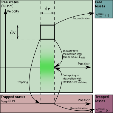
Figure 1: Phase-space diagram illustrating the collision, trapping, detrapping and recombination processes. (Source: (Stokes et al., 2016))

In this section, we consider a generalisation of the kinetic model presented in Eq. (1) from reference (Stokes et al., 2016) that describes the processes of collisions, trapping and recombination, as depicted in Fig. 1. Specifically, we make processes selective of particle energy $\epsilon\equiv\frac{1}{2}mv^{2}$. This results in a free particle phase-space distribution function $f\left(t,\mathbf{r},\mathbf{v}\right)$, defined by the generalised Boltzmann equation

$$\left(\frac{\partial}{\partial t}+\mathbf{v}\cdot\frac{\partial}{\partial\mathbf{r}}+\frac{e\mathbf{E}}{m}\cdot\frac{\partial}{\partial\mathbf{v}}\right)f\left(t,\mathbf{r},\mathbf{v}\right) = -\nu_{\mathrm{coll}}\left(\epsilon\right)f\left(t,\mathbf{r},\mathbf{v}\right)+n\left(t,\mathbf{r}\right)\left\langle\nu_{\mathrm{coll}}\left(\epsilon\right)\right\rangle\tilde{w}_{\mathrm{coll}}\left(v\right)$$ (1)

$$-\nu_{\mathrm{trap}}\left(\epsilon\right)f\left(t,\mathbf{r},\mathbf{v}\right)+\Phi\left(t\right)\ast\left[n\left(t,\mathbf{r}\right)\left\langle\nu_{\mathrm{trap}}\left(\epsilon\right)\right\rangle\right]\tilde{w}_{\mathrm{detrap}}\left(v\right)$$

$$-\nu_{\mathrm{loss}}^{\left(\mathrm{free}\right)}\left(\epsilon\right)f\left(t,\mathbf{r},\mathbf{v}\right),$$

which describes particles of charge $e$ and mass $m$ in the presence of an applied electric field $\mathbf{E}$. Here, the energy-dependent process rates for collisions, trapping and recombination losses are respectively denoted $\nu_{\mathrm{coll}}\left(\epsilon\right)$, $\nu_{\mathrm{trap}}\left(\epsilon\right)$, $\nu_{\mathrm{loss}}^{\left(\mathrm{free}\right)}\left(\epsilon\right)$, $\ast$ denotes a time convolution $\left\langle\cdot\right\rangle$ denotes an average over velocity space:

$$\left\langle\psi\left(\mathbf{v}\right)\right\rangle \equiv\frac{1}{n\left(t,\mathbf{r}\right)}\int\mathrm{d}\mathbf{v}\,f\left(t,\mathbf{r},\mathbf{v}\right)\psi\left(\mathbf{v}\right),$$ (2)

where the free particle number density is defined $n\left(t,\mathbf{r}\right)\equiv\int\mathrm{d}\mathbf{v}f\left(t,\mathbf{r},\mathbf{v}\right)$. Collisions are described above by the Bhatnagar-Gross-Krook (BGK) collision operator (Bhatnagar et al., 1954), while trapping and detrapping is described by a BGK-type model with a delay for the duration of each localised state (Philippa et al., 2014). This delay is sampled from the effective waiting time distribution (Stokes et al., 2016)

$$\Phi\left(t\right)\equiv\mathrm{e}^{-\nu_{\mathrm{loss}}^{\left(\mathrm{trap}\right)}t}\phi\left(t\right),$$ (3)

defined in terms of a distribution of trapping times $\phi\left(t\right)$ and weighted by an exponential decay term that describes the recombination of trapped particles at the rate $\nu_{\mathrm{loss}}^{\left(\mathrm{trap}\right)}$ (Stokes et al., 2016). Note that, unlike the free particle process rates, this recombination rate is not a function of energy as trapped particles are localised in space.

The processes of scattering and detrapping are taken to be isotropic and to occur according to Maxwellian velocity distributions. Specifically, we introduce

$$\tilde{w}_{\mathrm{coll}}\left(v\right) \equiv\frac{\nu_{\mathrm{coll}}\left(\epsilon\right)w\left(\alpha_{\mathrm{coll}},v\right)}{\int\mathrm{d}\mathbf{v}\nu_{\mathrm{coll}}\left(\epsilon\right)w\left(\alpha_{\mathrm{coll}},v\right)},$$ (4)

$$\tilde{w}_{\mathrm{detrap}}\left(v\right) \equiv\frac{\nu_{\mathrm{trap}}\left(\epsilon\right)w\left(\alpha_{\mathrm{detrap}},v\right)}{\int\mathrm{d}\mathbf{v}\nu_{\mathrm{trap}}\left(\epsilon\right)w\left(\alpha_{\mathrm{detrap}},v\right)},$$ (5)

where the Maxwellian velocity distribution of temperature $T$ is defined

$$w\left(\alpha,v\right) \equiv \left(\frac{\alpha^{2}}{2\pi}\right)^{\frac{3}{2}}\exp\left(-\frac{\alpha^{2}v^{2}}{2}\right),$$ (6)

$$\alpha^{2} \equiv \frac{m}{k_{\mathrm{B}}T},$$ (7)

where $k_{\mathrm{B}}$ is the Boltzmann constant.

As stated, this model is very general and requires the precise specification of atomic and molecular details to properly define the process frequencies. In practice, this is usually achieved by using cross-section data in the relationship $\nu\left(\epsilon\right)\equiv n_{0}v\sigma\left(\epsilon\right),$ where $n_{0}$ is the number density of the background medium and $\sigma\left(\epsilon\right)$ is the cross-section corresponding to the process of frequency $\nu\left(\epsilon\right)$.

Similar to the description of free particles by Eq. (1), trapped particles can be described by a distribution function in configuration space $n_{\mathrm{trap}}\left(t,\mathbf{r}\right)$, defined by the continuity equation

$$\frac{\partial}{\partial t}n_{\mathrm{trap}}\left(t,\mathbf{r}\right) = \left(1-\Phi\left(t\right)\ast\right)\left[n\left(t,\mathbf{r}\right)\left\langle\nu_{\mathrm{trap}}\left(\epsilon\right)\right\rangle\right]$$ (8)

$$-\nu_{\mathrm{loss}}^{\left(\mathrm{trap}\right)}n_{\mathrm{trap}}\left(t,\mathbf{r}\right).$$

Lastly, the number of particles lost to recombination can also be counted

$$\frac{\mathrm{d}}{\mathrm{d}t}N_{\mathrm{\mathrm{loss}}}^{\left(\mathrm{free}\right)}\left(t\right) = \left\langle\left\langle\nu_{\mathrm{loss}}^{\left(\mathrm{free}\right)}\left(\epsilon\right)\right\rangle\right\rangle N\left(t\right),$$ (9)

$$\frac{\mathrm{d}}{\mathrm{d}t}N_{\mathrm{\mathrm{loss}}}^{\left(\mathrm{trap}\right)}\left(t\right) = \nu_{\mathrm{loss}}^{\left(\mathrm{trap}\right)}N_{\mathrm{trap}}\left(t\right),$$ (10)

where $\left\langle\left\langle\cdot\right\rangle\right\rangle$ denotes an average over phase-space

$$\left\langle\left\langle\psi\right\rangle\right\rangle\equiv\frac{1}{N\left(t\right)}\int\mathrm{d}\mathbf{r}\int\mathrm{d}\mathbf{v}\,f\left(t,\mathbf{r},\mathbf{v}\right)\psi,$$ (11)

and free and trapped particle numbers are respectively defined

$$N\left(t\right) \equiv \int\mathrm{d}\mathbf{r}\,n\left(t,\mathbf{r}\right),$$ (12)

$$N_{\mathrm{trap}}\left(t\right) \equiv \int\mathrm{d}\mathbf{r\,}n_{\mathrm{trap}}\left(t,\mathbf{r}\right).$$ (13)

III Time-of-flight current transients

In practice, charged particle transport properties can be quantified using a time-of-flight experiment, where the transit time through a material for a pulse of charge carriers is found by measuring the corresponding current. In this section, we explore the impact that recombination losses of both delocalised and localised particles has on time-of-flight current transients. We consider the analytical current in a time-of-flight experiment for a material of thickness $L$ situated between two plane-parallel electrodes. As this geometry is one-dimensional, the charge carrier number density $n\left(t,x\right)$ is defined by the generalised diffusion equation derived in (Stokes et al., 2016), which is rewritten here:

$$\left\{\frac{\partial}{\partial t}+\nu_{\mathrm{trap}}\left[1-\Phi\left(t\right)\ast\right]+\nu_{\mathrm{loss}}^{\left(\mathrm{free}\right)}\right\}n+W\frac{\partial n}{\partial x}-D\frac{\partial^{2}n}{\partial x^{2}}=0,$$ (14)

where $W$ is the drift velocity and $D$ is the diffusion coefficient. This diffusion equation can be derived directly from the generalised Boltzmann equation (1), where the constant process frequencies can be interpreted as velocity averages of the energy-dependent frequencies introduced in the previous section, $\nu\equiv\left\langle\nu\left(\epsilon\right)\right\rangle$ . From the number density, the current in a time-of-flight experiment can be found as the spatially averaged flux (Philippa et al., 2011):

$$j\left(t\right)=e\frac{\partial}{\partial t}\int_{0}^{L}\left(\frac{x}{L}-1\right)n\left(t,x\right)\mathrm{d}x.$$ (15)

For an impulse initial condition, $n\left(0,x\right)=N\left(0\right)\delta\left(x-x_{0}\right)$, and perfectly absorbing boundaries, $n\left(t,0\right)=n\left(t,L\right)=0$, we can proceed as in (Philippa et al., 2014) to write this current in Laplace space:

$$j\left(p\right)=eN\left(0\right)\frac{W}{L\tilde{p}}\left\{1-\mathrm{e}^{-\lambda x_{0}}\left[\mathrm{e}^{-\beta x_{0}}+\frac{\sinh\left(\beta x_{0}\right)}{\sinh\left(\beta L\right)}\left(\mathrm{e}^{\lambda L}-\mathrm{e}^{-\beta L}\right)\right]\right\},$$ (16)

where

$$\tilde{p} \equiv p+\nu_{\mathrm{trap}}\left[1-\Phi\left(p\right)\right]+\nu_{\mathrm{loss}}^{\left(\mathrm{free}\right)},$$ (17)

$$\lambda \equiv \frac{W}{2D},$$ (18)

$$\beta \equiv \sqrt{\frac{\tilde{p}}{D}+\lambda^{2}},$$ (19)

and the Laplace transform of time, $t\rightarrow p$, is denoted $f\left(p\right)\equiv\mathcal{L}f\left(t\right)\equiv\int_{0}^{\infty}\mathrm{d}t\,\mathrm{e}^{-pt}f\left(t\right)$. Note that the trapped carrier recombination rate arises here through the term $\Phi\left(p\right)\equiv\phi\left(p+\nu_{\mathrm{loss}}^{\left(\mathrm{trap}\right)}\right).$

We consider the explicit effect that free and trapped particle recombination rates have on the current transient in a time-of-flight experiment in Fig. 2 by plotting Eq. (16) for the current, keeping the effects of mobility (drift velocity) and diffusion constant. A system of units is chosen that uses the material thickness $L$ and the trap-free transit time, defined as $t_{\mathrm{tr}}\equiv L/W$. In this system of units, the drift velocity is equal to unity. We specify the diffusion coefficient to be $Dt_{\mathrm{tr}}/L^{2}=0.02$, the initial impulse is set to occur at $x_{0}/L=1/3$ and the trapping rate is made large so as trap-based effects can occur within the transit time, $\nu_{\mathrm{trap}}t_{\mathrm{tr}}=10^{2}$. For trapping times, an exponential distribution is considered, $\phi\left(t\right)=\nu_{\mathrm{detrap}}\mathrm{e}^{-\nu_{\mathrm{detrap}}t}$, with a mean trapping time of $\left(\nu_{\mathrm{detrap}}t_{\mathrm{tr}}\right)^{-1}=0.03$.

In Fig. 2, the recombination-free current transient is included in black as a reference. This transient has a number of notable regimes. At early times, the current is still close to unity as no processes have had a chance to affect it greatly. What then follows is a decrease in current as free charge carriers enter traps. This decrease is temporary, however, and eventually the current plateaus as a transient equilibrium arises between free and trapped particles. The value of the current at this plateau is numerically equal to the proportion of free particles at the equilibrium, $\nu_{\mathrm{detrap}}/\left(\nu_{\mathrm{detrap}}+\nu_{\mathrm{trap}}\right)=0.25\approx 10^{-0.6}$. Finally, the last of the free particles extract causing the remaining filled traps to gradually exhaust and the system to leave equilibrium.

Fig. 2a) considers an increasing free particle recombination rate, $\nu_{\mathrm{loss}}^{\left(\mathrm{free}\right)}$, without any trapped particle recombination, $\nu_{\mathrm{loss}}^{\left(\mathrm{trap}\right)}=0$. It can be seen that the free particle losses start decreasing the current at roughly the characteristic time for free particle recombination, $\left(\nu_{\mathrm{loss}}^{\left(\mathrm{free}\right)}t_{\mathrm{tr}}\right)^{-1}$. Because free particles are being lost, an equilibrium is not established as in the recombination-free case. However, detrapping events do still cause a slowing in the descent of the current.

Fig. 2b) considers an increasing trapped particle recombination rate, $\nu_{\mathrm{loss}}^{\left(\mathrm{trap}\right)}$, without any free particle recombination, $\nu_{\mathrm{loss}}^{\left(\mathrm{free}\right)}=0$. Trap-based recombination can only affect the current via detrapping events and so we do not see a decrease in the current until at least the characteristic time for trapping, $\left(\nu_{\mathrm{trap}}t_{\mathrm{tr}}\right)^{-1}=10^{-2}$. Similar to Fig. 2a), an equilibrium cannot be established here due to the constant loss of trapped particles. Unlike Fig. 2a), however, detrapping events have a diminishing contribution to the current as increasing trap-based recombination also increases the probability that trapped particles recombine instead of detrapping.

In practice, time-of-flight current transients will be measured in experiments. These current traces will be fitted to solutions of the generalised diffusion equation (14), which enable the transport coefficients (drift velocity $W,$ diffusion coefficient $D$), various rates $\nu$ and the waiting time distribution $\phi$ to be determined empirically. In the remainder of this study, we are focussed on understanding the relationship between the various microscopic scattering and trapping processes (as determined by the relevant scattering, trapping and loss collision frequencies and their dependence on energy, and waiting time distributions) and the transport coefficients and properties. Furthermore, we will explore relationships between the transport coefficients/properties e.g. Wannier energy relation which links the mean energy and the mobility, and the generalised Einstein relations which link mobility and diffusivity.

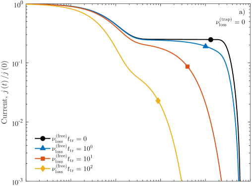
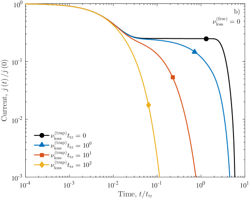
Figure 2: The impact of free and trapped particle recombination on current transients for an ideal time-of-flight experiment as modelled by Eq. (16). Nondimensionalisation has been performed using the material thickness $L$, trap-free transit time, $t_{\mathrm{tr}}\equiv L/W$, and the initial current $j\left(0\right)=eN\left(0\right)/t_{\mathrm{tr}}$. For these plots we define the diffusion coefficient, $Dt_{\mathrm{tr}}/L^{2}=0.02$, the initial impulse location, $x_{0}/L=1/3$, and the trapping rate, $\nu_{\mathrm{trap}}t_{\mathrm{tr}}=10^{2}$. We choose an exponential distribution of trapping times, $\phi\left(t\right)=\nu_{\mathrm{detrap}}\mathrm{e^{-\nu_{\mathrm{detrap}}t}}$, with the mean trapping time chosen as $\left(\nu_{\mathrm{detrap}}t_{\mathrm{tr}}\right)^{-1}=0.03$.

IV Balance equations

A knowledge of the full free particle phase-space distribution, $f(t,\mathbf{r},\mathbf{v})$, defined by the generalised Boltzmann equation (1), is often not required to analyse and interpret experiment. A computationally economical and more physically appealing alternative is to solve for average quantities directly, through solution of the appropriate fluid or velocity moment equations. In what follows, we form these moment equations by evaluating velocity averages of the phase-space distribution function, thus grounding them physically through the generalised Boltzmann equation.

From the Boltzmann equation (1), we show most generally that the average of a velocity functional $\psi\left(\mathbf{v}\right)$ satisfies the differential equation

$$\frac{\partial}{\partial t}n\left\langle\psi\right\rangle+\frac{\partial}{\partial\mathbf{r}}\cdot n\left\langle\mathbf{v}\psi\right\rangle-\frac{e\mathbf{E}}{m}\cdot n\left\langle\frac{\partial\psi}{\partial\mathbf{v}}\right\rangle = -n\left\langle\psi\nu_{\mathrm{coll}}\left(\epsilon\right)\right\rangle+n\left\langle\nu_{\mathrm{coll}}\left(\epsilon\right)\right\rangle\left\langle\psi\right\rangle_{\mathrm{coll}}$$ (20)

$$-n\left\langle\psi\nu_{\mathrm{trap}}\left(\epsilon\right)\right\rangle+\Phi\left(t\right)\ast\left(n\left\langle\nu_{\mathrm{trap}}\left(\epsilon\right)\right\rangle\right)\left\langle\psi\right\rangle_{\mathrm{detrap}}$$

$$-n\left\langle\psi\nu_{\mathrm{loss}}^{\left(\mathrm{free}\right)}\left(\epsilon\right)\right\rangle,$$

where the velocity average $\left\langle\cdot\right\rangle$ is defined by Eq. (2), while $\left\langle\cdot\right\rangle_{\mathrm{coll}}$ and $\left\langle\cdot\right\rangle_{\mathrm{detrap}}$ are defined as

$$\left\langle\psi\left(\mathbf{v}\right)\right\rangle_{\mathrm{coll}} \equiv\int\mathrm{d}\mathbf{v}\psi\left(\mathbf{v}\right)\tilde{w}_{\mathrm{coll}}\left(v\right),$$ (21)

$$\left\langle\psi\left(\mathbf{v}\right)\right\rangle_{\mathrm{detrap}} \equiv\int\mathrm{d}\mathbf{v}\psi\left(\mathbf{v}\right)\tilde{w}_{\mathrm{detrap}}\left(v\right).$$ (22)

By choosing $\psi\left(\mathbf{v}\right)=1$, $\psi\left(\mathbf{v}\right)=m\mathbf{v}$ and $\psi\left(\mathbf{v}\right)=\epsilon\equiv\frac{1}{2}mv^{2}$, respective balance equations for free particle continuity, momentum and energy result:

$$\frac{\partial}{\partial t}n+\frac{\partial}{\partial\mathbf{r}}\cdot n\left\langle\mathbf{v}\right\rangle = -n\left\langle\nu_{\mathrm{trap}}\left(\epsilon\right)\right\rangle+\Phi\left(t\right)\ast\left(n\left\langle\nu_{\mathrm{trap}}\left(\epsilon\right)\right\rangle\right)$$ (23)

$$-n\left\langle\nu_{\mathrm{loss}}^{\left(\mathrm{free}\right)}\left(\epsilon\right)\right\rangle,$$

$$\frac{\partial}{\partial t}n\left\langle m\mathbf{v}\right\rangle+\frac{\partial}{\partial\mathbf{r}}\cdot n\left\langle m\mathbf{v}\mathbf{v}\right\rangle-e\mathbf{E}n = -n\left\langle m\mathbf{v}\nu_{\mathrm{coll}}\left(\epsilon\right)\right\rangle$$ (24)

$$-n\left\langle m\mathbf{v}\nu_{\mathrm{trap}}\left(\epsilon\right)\right\rangle$$

$$-n\left\langle m\mathbf{v}\nu_{\mathrm{loss}}^{\left(\mathrm{free}\right)}\left(\epsilon\right)\right\rangle,$$

$$\frac{\partial}{\partial t}n\left\langle\epsilon\right\rangle+\frac{\partial}{\partial\mathbf{r}}\cdot n\left\langle\epsilon\mathbf{v}\right\rangle-e\mathbf{E}\cdot n\left\langle\mathbf{v}\right\rangle = -n\left\langle\epsilon\nu_{\mathrm{coll}}\left(\epsilon\right)\right\rangle+n\left\langle\nu_{\mathrm{coll}}\left(\epsilon\right)\right\rangle\left\langle\epsilon\right\rangle_{\mathrm{coll}}$$ (25)

$$-n\left\langle\epsilon\nu_{\mathrm{trap}}\left(\epsilon\right)\right\rangle+\Phi\left(t\right)\ast\left(n\left\langle\nu_{\mathrm{trap}}\left(\epsilon\right)\right\rangle\right)\left\langle\epsilon\right\rangle_{\mathrm{detrap}}$$

$$-n\left\langle\epsilon\nu_{\mathrm{loss}}^{\left(\mathrm{free}\right)}\left(\epsilon\right)\right\rangle.$$

The latter two equations can be written explicitly as differential equations in the average momentum and energy by expanding time derivatives and applying the continuity equation (23):

$$n\frac{\partial}{\partial t}\left\langle m\mathbf{v}\right\rangle+\frac{\partial}{\partial\mathbf{r}}\cdot n\left\langle m\mathbf{v}\mathbf{v}\right\rangle-\left\langle m\mathbf{v}\right\rangle\frac{\partial}{\partial\mathbf{r}}\cdot n\left\langle\mathbf{v}\right\rangle-e\mathbf{E}n = -n\left\langle m\mathbf{v}\nu_{\mathrm{coll}}\left(\epsilon\right)\right\rangle$$ (26)

$$-n\left\langle m\mathbf{v}\nu_{\mathrm{trap}}\left(\epsilon\right)\right\rangle+n\left\langle m\mathbf{v}\right\rangle\left\langle\nu_{\mathrm{trap}}\left(\epsilon\right)\right\rangle-\left\langle m\mathbf{v}\right\rangle\Phi\left(t\right)\ast\left(n\left\langle\nu_{\mathrm{trap}}\left(\epsilon\right)\right\rangle\right)$$

$$-n\left\langle m\mathbf{v}\nu_{\mathrm{loss}}^{\left(\mathrm{free}\right)}\left(\epsilon\right)\right\rangle+n\left\langle m\mathbf{v}\right\rangle\left\langle\nu_{\mathrm{loss}}^{\left(\mathrm{free}\right)}\left(\epsilon\right)\right\rangle,$$

$$n\frac{\partial}{\partial t}\left\langle\epsilon\right\rangle+\frac{\partial}{\partial\mathbf{r}}\cdot n\left\langle\epsilon\mathbf{v}\right\rangle-\left\langle\epsilon\right\rangle\frac{\partial}{\partial\mathbf{r}}\cdot n\left\langle\mathbf{v}\right\rangle-e\mathbf{E}\cdot n\left\langle\mathbf{v}\right\rangle = -n\left\langle\epsilon\nu_{\mathrm{coll}}\left(\epsilon\right)\right\rangle+n\left\langle\nu_{\mathrm{coll}}\left(\epsilon\right)\right\rangle\left\langle\epsilon\right\rangle_{\mathrm{coll}}$$ (27)

$$-n\left\langle\epsilon\nu_{\mathrm{trap}}\left(\epsilon\right)\right\rangle+n\left\langle\epsilon\right\rangle\left\langle\nu_{\mathrm{trap}}\left(\epsilon\right)\right\rangle-\left(\left\langle\epsilon\right\rangle-\left\langle\epsilon\right\rangle_{\mathrm{detrap}}\right)\Phi\left(t\right)\ast\left(n\left\langle\nu_{\mathrm{trap}}\left(\epsilon\right)\right\rangle\right)$$

$$-n\left\langle\epsilon\nu_{\mathrm{loss}}^{\left(\mathrm{free}\right)}\left(\epsilon\right)\right\rangle+n\left\langle\epsilon\right\rangle\left\langle\nu_{\mathrm{loss}}^{\left(\mathrm{free}\right)}\left(\epsilon\right)\right\rangle.$$

Solution of these balance equations requires some approximation in the evaluation of the averages of the collision frequencies. In what follows we solve these balance equations using momentum transfer theory (Robson, 1984) to develop expressions for the mobility, diffusion and the mean energy in terms of the underlying microscopic frequencies for collisions, trapping and losses. Application of these relationships yield some interesting phenomenon including negative differential conductivity (NDC) and heating/cooling, as well as conditions on the relevant frequencies for such phenomena to occur.

V Mobility and the Wannier energy relation: Heating/cooling and NDC

In this section, we are interested in physical properties in the weak-gradient hydrodynamic regime. In this limit, properties that are intensive (independent of particle number) become time invariant and spatial gradients vanish (Robson, 1986), resulting in simplified momentum and energy balance equations that provide expressions for the applied acceleration and power input by the field:

$$\frac{e\mathbf{E}}{m} = \left\langle\mathbf{v}\nu_{\mathrm{coll}}\left(\epsilon\right)\right\rangle^{\left(0\right)}$$ (28)

$$+\left\langle\mathbf{v}\nu_{\mathrm{trap}}\left(\epsilon\right)\right\rangle^{\left(0\right)}-\left(1-R\right)\mathbf{W}\left\langle\nu_{\mathrm{trap}}\left(\epsilon\right)\right\rangle^{\left(0\right)}$$

$$+\left\langle\mathbf{v}\nu_{\mathrm{loss}}^{\left(\mathrm{free}\right)}\left(\epsilon\right)\right\rangle^{\left(0\right)}-\mathbf{W}\left\langle\nu_{\mathrm{loss}}^{\left(\mathrm{free}\right)}\left(\epsilon\right)\right\rangle^{\left(0\right)},$$

$$e\mathbf{E}\cdot\mathbf{W} = \left\langle\epsilon\nu_{\mathrm{coll}}\left(\epsilon\right)\right\rangle^{\left(0\right)}-\left\langle\nu_{\mathrm{coll}}\left(\epsilon\right)\right\rangle^{\left(0\right)}\left\langle\epsilon\right\rangle_{\mathrm{coll}}$$ (29)

$$+\left\langle\epsilon\nu_{\mathrm{trap}}\left(\epsilon\right)\right\rangle^{\left(0\right)}-\varepsilon\left\langle\nu_{\mathrm{trap}}\left(\epsilon\right)\right\rangle^{\left(0\right)}+R\left\langle\nu_{\mathrm{trap}}\left(\epsilon\right)\right\rangle^{\left(0\right)}\left(\varepsilon-\left\langle\epsilon\right\rangle_{\mathrm{detrap}}\right)$$

$$+\left\langle\epsilon\nu_{\mathrm{loss}}^{\left(\mathrm{free}\right)}\left(\epsilon\right)\right\rangle^{\left(0\right)}-\varepsilon\left\langle\nu_{\mathrm{loss}}^{\left(\mathrm{free}\right)}\left(\epsilon\right)\right\rangle^{\left(0\right)}.$$

where the superscript “$\left(0\right)$” denotes that quantities are in the steady, spatially uniform state. Here, the moments for drift velocity and mean energy have been respectively defined

$$\mathbf{W} \equiv \left\langle\mathbf{v}\right\rangle^{\left(0\right)},$$ (30)

$$\varepsilon \equiv \left\langle\epsilon\right\rangle^{\left(0\right)},$$ (31)

and we have introduced the quantity $R$ as the steady-state ratio of the number of particles leaving traps to those entering traps:

$$R\equiv\left(\frac{\Phi\left(t\right)\ast n\left(t,\mathbf{r}\right)}{n\left(t,\mathbf{r}\right)}\right)^{\left(0\right)}\equiv\lim_{t\rightarrow\infty}\frac{\Phi\left(t\right)\ast N\left(t\right)}{N\left(t\right)}.$$ (32)

In the following subsections, we make these balance equations more useful by using momentum transfer theory to approximate the velocity averages of the form $\left\langle\nu\left(\epsilon\right)\right\rangle$, $\left\langle\mathbf{v}\nu\left(\epsilon\right)\right\rangle$ and $\left\langle\epsilon\nu\left(\epsilon\right)\right\rangle$. The simplified balance equations that result provide expressions for particle mobility and mean energy which in turn can be used to quantify heating/cooling and to explore NDC.

V.1 Momentum transfer theory

Momentum-transfer theory (Robson, 1984) enables a systematic procedure for evaluating the average rates detailed above. In this procedure, process rates, $\nu\left(\epsilon\right)$, are expanded about some representative energy, which we take to be the mean energy, $\varepsilon$:

$$\nu\left(\epsilon\right)=\sum_{i\geq 0}\frac{\nu^{\left(i\right)}\left(\varepsilon\right)}{i!}\left(\epsilon-\varepsilon\right)^{i},$$ (33)

where the superscript “$\left(i\right)$” denotes the $i$-th energy derivative. This expansion can then be truncated to the desired order of accuracy. By truncating to just the initial constant term, we have zeroth-order momentum transfer theory, which provides a mobility and a Wannier energy relation that is sufficient for exploring NDC and energy-independent heating/cooling. For heating/cooling that varies with energy, we must truncate the above expansion linearly and use first-order momentum transfer theory.

V.1.1 Zeroth-order momentum transfer theory

Truncating the energy expansion, Eq. (33), to the constant term gives the zeroth-order momentum transfer theory approximation

$$\left\langle\psi\left(\mathbf{v}\right)\nu\left(\epsilon\right)\right\rangle\approx\left\langle\psi\left(\mathbf{v}\right)\right\rangle\nu\left(\varepsilon\right).$$ (34)

This approximation yields results that are functionally equivalent to what arises for the case of constant process rates, as considered in (Stokes et al., 2016), but with some functional dependence on the representative energy $\varepsilon$. Substituting this approximation into the momentum and energy balance equations (24) and (25) yields

$$\frac{e\mathbf{E}}{m} = \mathbf{W}\nu_{\mathrm{eff}}\left(\varepsilon\right),$$ (35)

$$e\mathbf{E}\cdot\mathbf{W} = \left[\varepsilon-\frac{3}{2}k_{\mathrm{B}}T_{\mathrm{eff}}\left(\varepsilon\right)\right]\nu_{\mathrm{eff}}\left(\varepsilon\right),$$ (36)

where we have introduced an effective frequency

$$\nu_{\mathrm{eff}}\left(\varepsilon\right)\equiv\nu_{\mathrm{coll}}\left(\varepsilon\right)+R\nu_{\mathrm{trap}}\left(\varepsilon\right),$$ (37)

and an energy-dependent effective temperature, written as a weighted sum of the two Maxwellian source temperatures

$$T_{\mathrm{eff}}\left(\varepsilon\right)\equiv\omega_{\mathrm{coll}}\left(\varepsilon\right)T_{\mathrm{coll}}+\omega_{\mathrm{detrap}}\left(\varepsilon\right)T_{\mathrm{detrap}},$$ (38)

with energy-dependent weights defined

$$\omega_{\mathrm{coll}}\left(\varepsilon\right) \equiv \frac{\nu_{\mathrm{coll}}\left(\varepsilon\right)}{\nu_{\mathrm{coll}}\left(\varepsilon\right)+R\nu_{\mathrm{trap}}\left(\varepsilon\right)},$$ (39)

$$\omega_{\mathrm{trap}}\left(\varepsilon\right) \equiv \frac{R\nu_{\mathrm{trap}}\left(\varepsilon\right)}{\nu_{\mathrm{coll}}\left(\varepsilon\right)+R\nu_{\mathrm{trap}}\left(\varepsilon\right)}.$$ (40)

It should be noted that, as free particle recombination and trapping rates are constant here, the limit definition of $R$ in Eq. (32) can be evaluated to provide the alternative implicit definition (Stokes et al., 2016):

$$R\equiv\int_{0}^{\infty}\mathrm{d}t\,\Phi\left(t\right)\mathrm{e}^{\left[\nu_{\mathrm{loss}}^{\left(\mathrm{free}\right)}\left(\varepsilon\right)+\nu_{\mathrm{trap}}\left(\varepsilon\right)\left(1-R\right)\right]t}.$$ (41)

This implicit definition can be solved analytically for $R$ only for certain choices of the effective waiting time distribution $\Phi\left(t\right)$. A table of such $R$ values for a variety of corresponding $\Phi\left(t\right)$ is presented in Appendix A of (Stokes et al., 2016).

The zeroth-order momentum balance equation (35) provides the drift velocity in terms of the electric field $\mathbf{E}$:

$$\mathbf{W}\equiv K\mathbf{E},$$ (42)

where the constant of proportionality $K$ defines the charged particle mobility

$$K\equiv\frac{e}{m\nu_{\mathrm{eff}}\left(\varepsilon\right)}.$$ (43)

We observe that the mobility is inversely proportional to both collision and trapping process rates through the effective frequency defined in Eq. (37). This result is expected as both the scattering and detrapping processes occur isotropically. Evidently, precisely how mobility varies with energy depends entirely on the energy dependence of the process frequencies.

Using both the momentum and energy balance equations (35) and (36), we can also find the Wannier energy relation for the average energy

$$\varepsilon=\frac{3}{2}k_{\mathrm{B}}T_{\mathrm{eff}}\left(\varepsilon\right)+mW^{2}.$$ (44)

We can confirm that when there is no trapping, $\nu_{\mathrm{trap}}\left(\varepsilon\right)=0$, the mobility and Wannier energy relation reduce to the classical results valid for dilute gaseous systems (Robson, 1986):

$$K = \frac{e}{m\nu_{\mathrm{coll}}\left(\varepsilon\right)},$$ (45)

$$\varepsilon = \frac{3}{2}k_{\mathrm{B}}T_{\mathrm{coll}}+mW^{2}.$$ (46)

The zeroth-order mobility and Wannier energy relation derived here are used to describe energy-independent heating/cooling in Secs. V.2.1 and V.2.2 as well as NDC in Sec. V.3.

V.1.2 First-order momentum transfer theory

Including an additional term in the energy expansion, Eq. (33), gives the first-order momentum transfer theory approximation

$$\left\langle\psi\left(\mathbf{v}\right)\nu\left(\epsilon\right)\right\rangle\approx\left\langle\psi\left(\mathbf{v}\right)\right\rangle\nu\left(\varepsilon\right)+\left\langle\psi\left(\mathbf{v}\right)\left(\epsilon-\varepsilon\right)\right\rangle\nu^{\prime}\left(\varepsilon\right),$$ (47)

where $\nu^{\prime}\left(\varepsilon\right)$ denotes the energy derivative of $\nu\left(\varepsilon\right)$. Substitution into the momentum and energy balance equations (24) and (25) yields

$$\frac{e\mathbf{E}}{m} = \mathbf{W}\nu_{\mathrm{eff}}\left(\varepsilon\right)+\mathrm{cov}\left(\mathbf{v},\epsilon\right)\nu_{\mathrm{total}}^{\prime}\left(\varepsilon\right),$$ (48)

$$e\mathbf{E}\cdot\mathbf{W} = \left[\varepsilon-\frac{3}{2}k_{\mathrm{B}}T_{\mathrm{eff}}\left(\varepsilon\right)\right]\nu_{\mathrm{eff}}\left(\varepsilon\right)+\mathrm{var}\left(\epsilon\right)\nu_{\mathrm{total}}^{\prime}\left(\varepsilon\right)$$ (49)

$$-\frac{\frac{3}{2}\left(k_{\mathrm{B}}T_{\mathrm{coll}}\right)^{2}\nu_{\mathrm{coll}}^{\prime}\left(\varepsilon\right)}{1+\left(\frac{3}{2}k_{\mathrm{B}}T_{\mathrm{coll}}-\varepsilon\right)\frac{\nu_{\mathrm{coll}}^{\prime}\left(\varepsilon\right)}{\nu_{\mathrm{coll}}\left(\varepsilon\right)}}-\frac{\frac{3}{2}\left(k_{\mathrm{B}}T_{\mathrm{detrap}}\right)^{2}R\nu_{\mathrm{trap}}^{\prime}\left(\varepsilon\right)}{1+\left(\frac{3}{2}k_{\mathrm{B}}T_{\mathrm{detrap}}-\varepsilon\right)\frac{\nu_{\mathrm{trap}}^{\prime}\left(\varepsilon\right)}{\nu_{\mathrm{trap}}\left(\varepsilon\right)}},$$

where we define $\nu_{\mathrm{total}}\left(\varepsilon\right)\equiv\nu_{\mathrm{coll}}\left(\varepsilon\right)+\nu_{\mathrm{trap}}\left(\varepsilon\right)+\nu_{\mathrm{loss}}^{\left(\mathrm{free}\right)}\left(\varepsilon\right)$, and higher order velocity moments have been introduced in the form of the velocity-energy covariance

$$\mathrm{cov}\left(\mathbf{v},\epsilon\right)\equiv\left\langle\left(\mathbf{v}-\mathbf{W}\right)\left(\epsilon-\varepsilon\right)\right\rangle^{\left(0\right)}\equiv\boldsymbol{\xi}-\varepsilon\mathbf{W},$$ (50)

where $\boldsymbol{\xi}\equiv\left\langle\epsilon\mathbf{v}\right\rangle^{\left(0\right)}$ is the energy flux, and the energy variance

$$\mathrm{var}\left(\epsilon\right)\equiv\left\langle\left(\epsilon-\varepsilon\right)^{2}\right\rangle^{\left(0\right)}\equiv\left\langle\epsilon^{2}\right\rangle^{\left(0\right)}-\varepsilon^{2}.$$ (51)

These higher order velocity moments can be approximated using zeroth-order momentum transfer theory, as is done in Appendix A, to yield approximations expressed solely in terms of the lower order velocity moments $\mathbf{W}$ and $\varepsilon$. For example, the velocity-energy covariance can be approximated with

$$\mathrm{cov}\left(\mathbf{v},\epsilon\right)\approx\frac{2}{3}\left(\varepsilon+2mW^{2}\right)\mathbf{W}.$$ (52)

Using this approximation in conjunction with the first-order momentum balance equation (48), we find the mobility, as defined by Eq. (42):

$$K\approx\frac{e}{m\left[\nu_{\mathrm{eff}}\left(\varepsilon\right)+\frac{2}{3}\left(\varepsilon+2mW^{2}\right)\nu_{\mathrm{total}}^{\prime}\left(\varepsilon\right)\right]}.$$ (53)

This is of the same functional form as the zeroth-order mobility, Eq. (43), but with a modification to the effective frequency in the denominator. Note that the mobility now depends explicitly on the drift velocity, through the $2mW^{2}$ term. Terms such as this are sometimes omitted in the literature as their contribution is minimal when light particles are being considered (Robson, 1986).

As for zeroth-order momentum transfer theory, a Wannier energy relation can be formed by combining both momentum and energy balance equations (48) and (49):

$$\varepsilon =\frac{3}{2}k_{\mathrm{B}}T_{\mathrm{eff}}\left(\varepsilon\right)+mW^{2}$$

$$-\frac{\nu_{\mathrm{total}}^{\prime}\left(\varepsilon\right)}{\nu_{\mathrm{eff}}\left(\varepsilon\right)}\mathrm{cov}\left(\epsilon,\epsilon-m\mathbf{W}\cdot\mathbf{v}\right)+\frac{\frac{3}{2}\left(k_{\mathrm{B}}T_{\mathrm{coll}}\right)^{2}\frac{\nu_{\mathrm{coll}}^{\prime}\left(\varepsilon\right)}{\nu_{\mathrm{eff}}\left(\varepsilon\right)}}{1+\left(\frac{3}{2}k_{\mathrm{B}}T_{\mathrm{coll}}-\varepsilon\right)\frac{\nu_{\mathrm{coll}}^{\prime}\left(\varepsilon\right)}{\nu_{\mathrm{coll}}\left(\varepsilon\right)}}+\frac{\frac{3}{2}\left(k_{\mathrm{B}}T_{\mathrm{detrap}}\right)^{2}\frac{R\nu_{\mathrm{trap}}^{\prime}\left(\varepsilon\right)}{\nu_{\mathrm{eff}}\left(\varepsilon\right)}}{1+\left(\frac{3}{2}k_{\mathrm{B}}T_{\mathrm{detrap}}-\varepsilon\right)\frac{\nu_{\mathrm{trap}}^{\prime}\left(\varepsilon\right)}{\nu_{\mathrm{trap}}\left(\varepsilon\right)}}.$$ (54)

This first-order Wannier energy relation is written in terms of higher order velocity moments via the covariance

$$\mathrm{cov}\left(\epsilon,\epsilon-m\mathbf{W}\cdot\mathbf{v}\right)\equiv\mathrm{var}\left(\epsilon\right)-m\mathbf{W}\cdot\mathrm{cov}\left(\mathbf{v},\epsilon\right).$$ (55)

As before, the results in Appendix A allow for this covariance to also be written approximately in terms of lower order velocity moments:

$$\mathrm{cov}\left(\epsilon,\epsilon-m\mathbf{W}\cdot\mathbf{v}\right)\approx\frac{2}{3}\left(\varepsilon-\frac{1}{2}mW^{2}\right)^{2}+\frac{17}{6}\left(mW^{2}\right)^{2}+\frac{5}{3}\omega_{\mathrm{coll}}\left(\varepsilon\right)\omega_{\mathrm{trap}}\left(\varepsilon\right)\left[\frac{3}{2}k_{\mathrm{B}}\left(T_{\mathrm{coll}}-T_{\mathrm{detrap}}\right)\right]^{2}.$$ (56)

This expression can be used to write the first-order Wannier energy relation (54) in an approximate closed form, independent of higher order velocity moments.

Comparing the above first-order momentum transfer theory results for mobility and average energy, Eqs. (53) and (54), to their zeroth-order counterparts, Eqs. (43) and (44), provides an estimate of the error incurred by the zeroth-order momentum transfer theory approximation.

In Sec. V.2.3, we use the first-order mobility and Wannier energy relation derived here to describe heating/cooling that is due to the energy dependence of physical processes.

V.2 Heating and cooling

In this subsection, we determine the effect that each of the physical processes described by the generalised Boltzmann equation (1) have on the average particle energy. That is, whether there is an increase or decrease in the average energy corresponding to a respective heating or cooling of the particles as a result of collisions, trapping or recombination.

V.2.1 Collisional and trap-based heating/cooling

To consider the effect of collisions on the average energy, we consider the case of constant process rates where the average energy is given by the zeroth-order Wannier energy relation (44). For collisions that are infrequent relative to trapping, i.e. $\nu_{\mathrm{coll}}<R\nu_{\mathrm{trap}}$, the average energy can be written approximately to first order in $\nu_{\mathrm{coll}}/R\nu_{\mathrm{trap}}$:

$$\varepsilon\approx\varepsilon_{0}+2\left(\frac{3}{2}k_{\mathrm{B}}T_{\mathrm{HC}}-\varepsilon_{0}\right)\frac{\nu_{\mathrm{coll}}}{R\nu_{\mathrm{trap}}},$$ (57)

where the subscript “$0$” denotes the collisionless case, i.e. $\nu_{\mathrm{coll}}=0$:

$$\varepsilon_{0} = \frac{3}{2}k_{\mathrm{B}}T_{\mathrm{detrap}}+mW_{0}^{2},$$ (58)

$$\mathbf{W}_{0} = \frac{e\mathbf{E}}{mR\nu_{\mathrm{trap}}},$$ (59)

and $T_{\mathrm{HC}}$ is a threshold temperature which defines the transition between collisional heating and cooling:

$$T_{\mathrm{HC}}\equiv\frac{T_{\mathrm{coll}}+T_{\mathrm{detrap}}}{2}.$$ (60)

In the event that $\varepsilon_{0}=\frac{3}{2}k_{\mathrm{B}}T_{\mathrm{HC}}$, the first order term in the expansion above vanishes and we must instead consider the second-order approximation:

$$\varepsilon\approx\varepsilon_{0}+mW_{0}^{2}\left(\frac{\nu_{\mathrm{coll}}}{R\nu_{\mathrm{trap}}}\right)^{2}.$$ (61)

The expansions (57) and (61) show that the introduction of collisions cause cooling only if the initial average energy $\varepsilon_{0}$ exceeds the threshold energy proportional to the temperature $T_{\mathrm{HC}}$:

$$\varepsilon_{0}>\frac{3}{2}k_{\mathrm{B}}T_{\mathrm{HC}},$$ (62)

with collisional heating occurring otherwise.

These conditions can also be shown to be applicable to trap-based heating/cooling, in which case $\varepsilon_{0}$ would denote the trap-free mean energy with $\nu_{\mathrm{trap}}=0$.

V.2.2 Energy-indiscriminate recombination heating/cooling

We now explore the possibility of recombination heating/cooling by once again considering constant process rates. It is usually expected that constant loss rates, which act indiscriminate of energy, result in a decrease in particle number that affects extensive properties but leaves intensive properties, like the average energy, unchanged (Robson, 1986). Although it is true that the recombination considered here is not selective of particle energy, the separate recombination rates for free and trapped particles means that recombination is selective of whether particles are trapped or not. Indeed, the average energy can be shown to be a function of the difference in these recombination rates, $\Delta\nu_{\mathrm{loss}}\equiv\nu_{\mathrm{loss}}^{\left(\mathrm{free}\right)}-\nu_{\mathrm{loss}}^{\left(\mathrm{trap}\right)}$, only becoming independent when recombination acts uniformly across all particles, i.e. $\nu_{\mathrm{loss}}^{\left(\mathrm{free}\right)}=\nu_{\mathrm{loss}}^{\left(\mathrm{trap}\right)}$. The recombination dependence appears in the average energy through the quantity $R$, whose definition in Eq. (41) is rewritten here explicitly in terms of $\Delta\nu_{\mathrm{loss}}$:

$$R\equiv\int_{0}^{\infty}\mathrm{d}t\,\phi\left(t\right)\mathrm{e}^{\left[\Delta\nu_{\mathrm{loss}}+\nu_{\mathrm{trap}}\left(1-R\right)\right]t}.$$ (63)

The original definition of $R$ was given by Eq. (32) as the steady-state ratio between the number of particles leaving and entering traps. Without recombination, this ratio is unity as an equilibrium arises between free and trapped particles (Stokes et al., 2016). Even with recombination, this ratio should remain at unity so long as the number of free and trapped particles reduce equally due to recombination, $\Delta\nu_{\mathrm{loss}}=0$.

We explore the effect of $R$ on heating/cooling by performing a small $\Delta\nu_{\mathrm{loss}}$ expansion:

$$R\approx 1+\frac{\Delta\nu_{\mathrm{loss}}}{\nu_{\mathrm{detrap}}+\nu_{\mathrm{trap}}},$$ (64)

where the detrapping rate has been introduced

$$\nu_{\mathrm{detrap}}^{-1}\equiv\int_{0}^{\infty}\mathrm{d}t\,\phi\left(t\right)t.$$ (65)

Proceeding to perform a small $\Delta\nu_{\mathrm{loss}}$ expansion of the average energy, in part by using the above expansion of $R$, gives the average energy to first order:

$$\varepsilon\approx\varepsilon_{0}+2\left(\frac{3}{2}k_{\mathrm{B}}T_{\mathrm{HC}}-\varepsilon_{0}\right)\frac{\nu_{\mathrm{trap}}}{\nu_{\mathrm{coll}}+\nu_{\mathrm{trap}}}\frac{\Delta\nu_{\mathrm{loss}}}{\nu_{\mathrm{detrap}}+\nu_{\mathrm{trap}}},$$ (66)

where the subscript “$0$” denotes the case of uniform recombination, $\Delta\nu_{\mathrm{loss}}=0$:

$$\varepsilon_{0} = \frac{3}{2}k_{\mathrm{B}}T_{\mathrm{eff,0}}+mW_{0}^{2},$$ (67)

$$\mathbf{W}_{0} = \frac{e\mathbf{E}}{m\left(\nu_{\mathrm{coll}}+\nu_{\mathrm{trap}}\right)},$$ (68)

$$T_{\mathrm{eff,0}} = \frac{\nu_{\mathrm{coll}}T_{\mathrm{coll}}+\nu_{\mathrm{trap}}T_{\mathrm{detrap}}}{\nu_{\mathrm{coll}}+\nu_{\mathrm{trap}}},$$ (69)

and the threshold temperature in this case is defined as

$$T_{\mathrm{HC}}\equiv\frac{T_{\mathrm{eff},0}+T_{\mathrm{detrap}}}{2}.$$ (70)

In the event that $\varepsilon_{0}=\frac{3}{2}k_{\mathrm{B}}T_{\mathrm{HC}}$, we have instead the second-order approximation for average energy:

$$\varepsilon\approx\varepsilon_{0}+mW_{0}^{2}\left(\frac{\nu_{\mathrm{trap}}}{\nu_{\mathrm{coll}}+\nu_{\mathrm{trap}}}\frac{\Delta\nu_{\mathrm{loss}}}{\nu_{\mathrm{detrap}}+\nu_{\mathrm{trap}}}\right)^{2},$$ (71)

From the small $\Delta\nu_{\mathrm{loss}}$ expansions (66) and (71), we see that if there is a relative loss of free particles, $\nu_{\mathrm{loss}}^{\left(\mathrm{free}\right)}>\nu_{\mathrm{loss}}^{\left(\mathrm{trap}\right)}$, then recombination cooling can occur if those free particles are sufficiently energetic prior to being lost:

$$\varepsilon_{0}>\frac{3}{2}k_{\mathrm{B}}T_{\mathrm{HC}}.$$ (72)

Conversely, if there is a relative gain of free particles, $\nu_{\mathrm{loss}}^{\left(\mathrm{free}\right)}<\nu_{\mathrm{loss}}^{\left(\mathrm{trap}\right)}$, then recombination cooling can occur if those free particles are sufficiently cold to begin with:

$$\varepsilon_{0}<\frac{3}{2}k_{\mathrm{B}}T_{\mathrm{HC}}.$$ (73)

Overall, for distinct free and trapped particle recombination rates such that $\nu_{\mathrm{loss}}^{\left(\mathrm{free}\right)}\neq\nu_{\mathrm{loss}}^{\left(\mathrm{trap}\right)}$, the condition for recombination cooling can be summarised as

$$\left(\varepsilon_{0}-\frac{3}{2}k_{\mathrm{B}}T_{\mathrm{HC}}\right)\Delta\nu_{\mathrm{loss}}>0,$$ (74)

with recombination heating occurring otherwise.

V.2.3 Energy-selective recombination heating/cooling

In the event that no traps are present, $\nu_{\mathrm{trap}}=0$, or where recombination acts uniformly across all free and trapped particles, $\nu_{\mathrm{loss}}^{\left(\mathrm{free}\right)}=\nu_{\mathrm{loss}}^{\left(\mathrm{trap}\right)}$, heating and cooling can not occur due to the trap-selective recombination described in the previously. In this case, heating or cooling can only occur if recombination acts selectively based on the energy of the free particles. To show this, we will consider the first-order Wannier energy relation (54) with constant collision and trapping rates and constant free particle recombination rate energy derivative $\nu_{\mathrm{loss}}^{\left(\mathrm{free}\right)\prime}$. Performing a small $\nu_{\mathrm{loss}}^{\left(\mathrm{free}\right)\prime}/\nu_{\mathrm{eff}}$ expansion of this average energy gives, to first order:

$$\varepsilon\approx\varepsilon_{0}-\left\{\frac{2}{3}\left(\varepsilon_{0}+\frac{1}{2}mW_{0}^{2}\right)^{2}+\frac{11}{2}\left(mW_{0}^{2}\right)^{2}+\frac{5}{3}\omega_{\mathrm{coll}}\omega_{\mathrm{trap}}\left[\frac{3}{2}k_{\mathrm{B}}\left(T_{\mathrm{coll}}-T_{\mathrm{detrap}}\right)\right]^{2}\right\}\frac{\nu_{\mathrm{loss}}^{\left(\mathrm{free}\right)\prime}}{\nu_{\mathrm{eff}}},$$ (75)

where the subscript “$0$” denotes no energy dependence in the free particle recombination rate, $\nu_{\mathrm{loss}}^{\left(\mathrm{free}\right)\prime}=0$:

$$\varepsilon_{0} = \frac{3}{2}k_{\mathrm{B}}T_{\mathrm{eff}}+mW_{0}^{2},$$ (76)

$$\mathbf{W}_{0} = \frac{e\mathbf{E}}{m\nu_{\mathrm{eff}}}.$$ (77)

As is expected, the expansion (75) suggests that recombination cooling occurs when recombination is selective of higher energy particles,

$$\nu_{\mathrm{loss}}^{\left(\mathrm{free}\right)\prime}>0,$$ (78)

with recombination heating occurring when it is selective of lower energy particles. This confirms for this model the well known phenomena of attachment heating/cooling (Robson, 1986).

V.3 Negative differential conductivity

Negative differential conductivity (NDC) occurs when an increase in field strength causes a decrease in the drift velocity (Robson, 1984):

$$\frac{\mathrm{d}W}{\mathrm{d}E}<0.$$ (79)

The field rate of change of drift velocity can be found directly from the zeroth-order Wannier energy relation (44) as

$$\frac{\mathrm{d}W}{\mathrm{d}E}=\frac{1}{2mW}\left[1-\frac{3}{2}k_{\mathrm{B}}T_{\mathrm{eff}}^{\prime}\left(\varepsilon\right)\right]\frac{\mathrm{d}\varepsilon}{\mathrm{d}E},$$ (80)

which provides the condition for the occurrence of NDC:

$$\frac{3}{2}k_{\mathrm{B}}T_{\mathrm{eff}}^{\prime}\left(\varepsilon\right)>1.$$ (81)

The NDC condition assumes that the mean energy increases monotonically with the field

$$\frac{\mathrm{d}\varepsilon}{\mathrm{d}E}>0.$$ (82)

This is equivalent to restricting the effective frequency $\nu_{\mathrm{eff}}\left(\varepsilon\right)$ so as to avoid runaway and ensure that an equilibrium is reached (Skullerud and Forsth, 1979):

$$\frac{\mathrm{d}}{\mathrm{d}\varepsilon}\left(\nu_{\mathrm{eff}}\left(\varepsilon\right)\sqrt{\varepsilon-\frac{3}{2}k_{\mathrm{B}}T_{\mathrm{eff}}\left(\varepsilon\right)}\right)>0.$$ (83)

Note that the occurrence of NDC depends solely on how the effective temperature varies with energy. This energy rate of change is proportional to the difference in Maxwellian temperatures:

$$T_{\mathrm{eff}}^{\prime}\left(\varepsilon\right)=\left(T_{\mathrm{coll}}-T_{\mathrm{detrap}}\right)\omega_{\mathrm{coll}}^{\prime}\left(\varepsilon\right)=\left(T_{\mathrm{detrap}}-T_{\mathrm{coll}}\right)\omega_{\mathrm{trap}}^{\prime}\left(\varepsilon\right).$$ (84)

Hence, in comparison with Eq. (81), we see that NDC here cannot occur when both scattering and detrapping sources are of equal temperature or when the relative collision or trapping rates, $\omega_{\mathrm{coll}}\left(\varepsilon\right)$ and $\omega_{\mathrm{trap}}\left(\varepsilon\right)$ , do not vary rapidly enough with mean energy.

Fig. 3 plots both the drift velocity $W$ and mean energy $\varepsilon$ as functions of the applied electric field $E$ for a situation in which NDC arises. Previous studies (Petrovic et al., 1984; Robson, 1984) found that, for inelastic processes, the signature of NDC is a rapidly-increasing mean energy. Interestingly, the opposite is true in the example considered for our model, with the mean energy plateauing when NDC occurs. This contrast can be understood by considering the frequency that defines the mobility in each case. For NDC to occur, this frequency must increase sufficiently quickly with applied field. In the referenced studies this frequency increases over a range of energies, causing the mean energy to increase rapidly through this range when NDC occurs. However, in our example in Fig. 3, the effective frequency increases rapidly at a particular energy, causing the mean energy to plateau at this energy during the NDC regime.

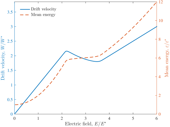
Figure 3: Plots of drift velocity, Eq. (42), and mean energy, Eq. (44), against electric field for a situation in which negative differential conductivity arises. All quantities have been nondimensionalised with respect to the mean energy without a field applied, $\varepsilon^{\star}\equiv\frac{3}{2}k_{\mathrm{B}}T_{\mathrm{eff}}\left(\varepsilon^{\star}\right)$. Specifically, we have chosen to nondimensionalise using $W^{\star}\equiv\sqrt{\frac{\varepsilon^{\star}}{m}}$ and $E^{\star}\equiv\frac{m\nu_{\mathrm{eff}}\left(\varepsilon^{\star}\right)}{e}W^{\star}$. For this figure, we consider a constant collision frequency, $\nu_{\mathrm{coll}}\left(\varepsilon\right)=1$, and a trapping frequency that approximates a step function, $R\nu_{\mathrm{trap}}\left(\varepsilon\right)=\frac{1}{2}\left\{1+\tanh\left[5\left(\varepsilon-\varepsilon_{\mathrm{thresh}}\right)\right]\right\}\approx H\left(\varepsilon-\varepsilon_{\mathrm{thresh}}\right)$, turning on at the threshold energy $\varepsilon_{\mathrm{thresh}}=6$. In addition, Maxwellian temperatures have been chosen such that $k_{\mathrm{B}}T_{\mathrm{coll}}=1$ and $k_{\mathrm{B}}T_{\mathrm{detrap}}=5$.

VI Diffusion: Generalised Einstein relations and anisotropy

In this section, we form a generalisation of the classical Einstein relation between diffusivity $\mathbf{D}$ and temperature $\mathbf{T}$ tensors (Einstein, 1905):

$$\frac{\mathbf{D}}{K}=\frac{k_{\mathrm{B}}\mathbf{T}}{e},$$ (85)

for the phase-space model described by Eq. (1). To do this, we make use of Fick’s law:

$$\left\langle\mathbf{v}\right\rangle\approx\mathbf{W}-\mathbf{D}\cdot\frac{1}{n}\frac{\partial n}{\partial\mathbf{r}}.$$ (86)

The use of Fick’s law here is justified in (Stokes et al., 2016) where it is shown that velocity averages can be written in the weak-gradient hydrodynamic regime as a density gradient expansion

$$\left\langle\psi\right\rangle=\left\langle\psi\right\rangle^{\left(0\right)}+\left\langle\psi\right\rangle^{\left(1\right)}\cdot\frac{1}{n}\frac{\partial n}{\partial\mathbf{r}}+\left\langle\psi\right\rangle^{\left(2\right)}\colon\frac{1}{n}\frac{\partial^{2}n}{\partial\mathbf{r}\partial\mathbf{r}}+\cdots.$$ (87)

To find an expression for the diffusion coefficient, we must apply density gradient expansions to all average quantities in the momentum and energy balance equations (24) and (25). For the mean energy we have, to first spatial order (Stokes et al., 2016)

$$\left\langle\epsilon\right\rangle\approx\varepsilon+\boldsymbol{\gamma}\cdot\frac{1}{n}\frac{\partial n}{\partial\mathbf{r}},$$ (88)

where $\boldsymbol{\gamma}$ is the energy gradient parameter. Using the density gradient expansions of average velocity and energy, Eqs. (86) and (88), we can determine the following density gradient expansions valid for an arbitrary frequency $\nu\left(\epsilon\right)$:

$$\left\langle\nu\left(\epsilon\right)\right\rangle \approx \nu\left(\varepsilon\right)+\nu^{\prime}\left(\varepsilon\right)\boldsymbol{\gamma}\cdot\frac{1}{n}\frac{\partial n}{\partial\mathbf{r}},$$ (89)

$$\left\langle\mathbf{v}\nu\left(\epsilon\right)\right\rangle \approx \mathbf{W}\nu\left(\varepsilon\right)+\left[\nu^{\prime}\left(\varepsilon\right)\boldsymbol{\gamma}\mathbf{W}-\nu\left(\varepsilon\right)\mathbf{D}\right]\cdot\frac{1}{n}\frac{\partial n}{\partial\mathbf{r}},$$ (90)

$$\left\langle\epsilon\nu\left(\epsilon\right)\right\rangle \approx \varepsilon\nu\left(\varepsilon\right)+\left[\nu\left(\varepsilon\right)+\varepsilon\nu^{\prime}\left(\varepsilon\right)\right]\boldsymbol{\gamma}\cdot\frac{1}{n}\frac{\partial n}{\partial\mathbf{r}}.$$ (91)

Lastly, we also perform the density gradient expansion of the concentration of particles leaving traps

$$\Phi\left(t\right)\ast n\left(t,\mathbf{r}\right)\approx Rn+\mathbf{R}^{\left(1\right)}\cdot\frac{\partial n}{\partial\mathbf{r}},$$ (92)

where $R$ is defined by Eq. (41) as the steady-state ratio between the number of particles leaving and entering traps, and $\mathbf{R}^{\left(1\right)}$ is a vector that has a component due to the energy dependence of $R$ and an intrinsic component present even for constant process rates, as was found in Eq. (71) of (Stokes et al., 2016):

$$\mathbf{R}^{\left(1\right)} \equiv R^{\prime}\left(\varepsilon\right)\boldsymbol{\gamma}+\frac{R\tau}{1+\nu_{\mathrm{trap}}\left(\varepsilon\right)R\tau}\mathbf{W},$$ (93)

where we define an average time

$$\tau\equiv\frac{1}{R}\int_{0}^{\infty}\mathrm{d}t\,\Phi\left(t\right)\mathrm{e}^{\left[\nu_{\mathrm{loss}}^{\left(\mathrm{free}\right)}\left(\varepsilon\right)+\nu_{\mathrm{trap}}\left(\varepsilon\right)\left(1-R\right)\right]t}t,$$ (94)

which coincides with the mean trapping time when the free and trapped particle recombination rates coincide, $\nu_{\mathrm{loss}}^{\left(\mathrm{free}\right)}\left(\varepsilon\right)=\nu_{\mathrm{loss}}^{\left(\mathrm{trap}\right)}$.

The weak-gradient hydrodynamic regime balance equations can now be considered to first spatial order by applying all of the above density gradient expansions. Doing so and equating first-order terms yields

$$\frac{k_{\mathrm{B}}\mathbf{T}}{m} = \nu_{\mathrm{eff}}\left(\varepsilon\right)\mathbf{D}-\nu_{\mathrm{eff}}^{\prime}\left(\varepsilon\right)\boldsymbol{\gamma}\mathbf{W}-\frac{\nu_{\mathrm{trap}}\left(\varepsilon\right)R\tau}{1+\nu_{\mathrm{trap}}\left(\varepsilon\right)R\tau}\mathbf{W}\mathbf{W},$$ (95)

$$-\frac{\mathbf{Q}}{\nu_{\mathrm{eff}}\left(\varepsilon\right)} = \left[1-\frac{3}{2}k_{\mathrm{B}}T_{\mathrm{eff}}^{\prime}\left(\varepsilon\right)\right]\boldsymbol{\gamma}+2m\mathbf{W}\cdot\mathbf{D}$$ (96)

$$+\frac{3}{2}k_{\mathrm{B}}\left(T_{\mathrm{coll}}-T_{\mathrm{detrap}}\right)\omega_{\mathrm{coll}}\left(\varepsilon\right)\omega_{\mathrm{detrap}}\left(\varepsilon\right)\frac{R\tau}{1+\nu_{\mathrm{trap}}\left(\varepsilon\right)R\tau}\mathbf{W},$$

where the temperature $\mathbf{T}$ and heat flux $\mathbf{Q}$ are defined in terms of the peculiar velocity $\mathbf{V}\equiv\mathbf{v}-\mathbf{W}$ as

$$k_{\mathrm{B}}\mathbf{T} \equiv m\left\langle\mathbf{V}\mathbf{V}\right\rangle^{\left(0\right)},$$ (97)

$$\mathbf{Q} \equiv \frac{1}{2}m\left\langle V^{2}\mathbf{V}\right\rangle^{\left(0\right)}.$$ (98)

By writing the above system of equations in terms of components of diffusivity and temperature perpendicular and parallel to the field:

$$\mathbf{D} \equiv D_{\perp}\left(\mathbf{I}-\hat{\mathbf{E}}\hat{\mathbf{E}}\right)+D_{\parallel}\hat{\mathbf{E}}\hat{\mathbf{E}},$$ (99)

$$\mathbf{T} \equiv T_{\perp}\left(\mathbf{I}-\hat{\mathbf{E}}\hat{\mathbf{E}}\right)+T_{\parallel}\hat{\mathbf{E}}\hat{\mathbf{E}},$$ (100)

and solving for each component of diffusivity separately yields the generalised Einstein relations

$$D_{\perp} = \frac{k_{\mathrm{B}}T_{\perp}}{m\nu_{\mathrm{eff}}\left(\varepsilon\right)},$$ (101)

$$D_{\parallel} = \frac{k_{\mathrm{B}}T_{\parallel}+mW^{2}\frac{\nu_{\mathrm{trap}}\left(\varepsilon\right)R\tau}{1+\nu_{\mathrm{trap}}\left(\varepsilon\right)R\tau}-\left[\frac{Q}{W}+\frac{3}{2}k_{\mathrm{B}}\left(T_{\mathrm{coll}}-T_{\mathrm{detrap}}\right)\frac{\nu_{\mathrm{coll}}\left(\varepsilon\right)}{\nu_{\mathrm{eff}}\left(\varepsilon\right)}\frac{\nu_{\mathrm{trap}}\left(\varepsilon\right)R\tau}{1+\nu_{\mathrm{trap}}\left(\varepsilon\right)R\tau}\right]\frac{mW^{2}}{1-\frac{3}{2}k_{\mathrm{B}}T_{\mathrm{eff}}^{\prime}\left(\varepsilon\right)}\frac{\nu_{\mathrm{eff}}^{\prime}\left(\varepsilon\right)}{\nu_{\mathrm{eff}}\left(\varepsilon\right)}}{m\nu_{\mathrm{eff}}\left(\varepsilon\right)\left(1+\frac{2mW^{2}}{1-\frac{3}{2}k_{\mathrm{B}}T_{\mathrm{eff}}^{\prime}\left(\varepsilon\right)}\frac{\nu_{\mathrm{eff}}^{\prime}\left(\varepsilon\right)}{\nu_{\mathrm{eff}}\left(\varepsilon\right)}\right)}.$$ (102)

Using the zeroth-order mobility and Wannier energy relation derived in Sec. V.1.1, we find the identity:

$$\frac{\frac{\mathrm{d}\ln K}{\mathrm{d}\ln E}}{1+\frac{\mathrm{d}\ln K}{\mathrm{d}\ln E}}\equiv-\frac{2mW^{2}}{1-\frac{3}{2}k_{\mathrm{B}}T_{\mathrm{eff}}^{\prime}\left(\varepsilon\right)}\frac{\nu_{\mathrm{eff}}^{\prime}\left(\varepsilon\right)}{\nu_{\mathrm{eff}}\left(\varepsilon\right)},$$ (103)

which allows the above generalised Einstein relations to be written in terms of the field-dependence of the mobility $K$:

$$\frac{D_{\perp}}{K} = \frac{k_{\mathrm{B}}T_{\perp}}{e},$$ (104)

$$\frac{D_{\parallel}}{K} = \frac{k_{\mathrm{B}}T_{\parallel}+mW^{2}\frac{\nu_{\mathrm{trap}}\left(\varepsilon\right)R\tau}{1+\nu_{\mathrm{trap}}\left(\varepsilon\right)R\tau}}{e}\left[1+\left(1+\Delta\right)\frac{\mathrm{d}\ln K}{\mathrm{d}\ln E}\right],$$ (105)

where

$$\Delta\equiv\frac{Q+\frac{3}{2}k_{\mathrm{B}}\left(T_{\mathrm{coll}}-T_{\mathrm{detrap}}\right)W\frac{\nu_{\mathrm{coll}}\left(\varepsilon\right)}{\nu_{\mathrm{eff}}\left(\varepsilon\right)}\frac{\nu_{\mathrm{trap}}\left(\varepsilon\right)R\tau}{1+\nu_{\mathrm{trap}}\left(\varepsilon\right)R\tau}}{2k_{\mathrm{B}}T_{\parallel}W+2mW^{3}\frac{\nu_{\mathrm{trap}}\left(\varepsilon\right)R\tau}{1+\nu_{\mathrm{trap}}\left(\varepsilon\right)R\tau}}.$$ (106)

We can see that the perpendicular generalised Einstein relation coincides with the classical Einstein relation (85) and that the parallel one deviates from it, highlighting the anisotropic nature of diffusion. In the case where there is no trapping, $\nu_{\mathrm{trap}}\left(\varepsilon\right)=0$, the above parallel Einstein relation reduces to

$$\frac{D_{\parallel}}{K} = \frac{k_{\mathrm{B}}T_{\parallel}}{e}\left[1+\left(1+\Delta\right)\frac{\mathrm{d}\ln K}{\mathrm{d}\ln E}\right],$$ (107)

with

$$\Delta\equiv\frac{Q}{2k_{\mathrm{B}}T_{\parallel}W},$$ (108)

which coincides with the well-known gas-phase results (Robson, 1976, 1984). The deviation of this collision-only generalised Einstein relation (107) from the classical Einstein relation (85) is due entirely to the energy dependence of the process rates. Interestingly, this is not the case when trapping is considered, as choosing constant process rates for the generalised Einstein relation (105) results in a parallel diffusion coefficient that still has some enhancement:

$$\frac{D_{\parallel}}{K}=\frac{k_{\mathrm{B}}T_{\parallel}+mW^{2}\frac{\nu_{\mathrm{trap}}R\tau}{1+\nu_{\mathrm{trap}}R\tau}}{e}.$$ (109)

This anisotropy is to be expected as, rather than moving with the applied field, some particles become localised in traps only to detrap later to contribute to the spread of free particles.

VII Consequences of fractional transport

In our previous works (Philippa et al., 2014; Stokes et al., 2016) it was shown that, for certain choices of the trapping time distribution $\phi\left(t\right)$, the phase-space model defined in Sec. II can be described by a diffusion equation with a time derivative of non-integer order. Specifically, given an effective trapping time distribution with a heavy tail of the form

$$\Phi\left(t\right)\sim t^{-\left(1+\alpha\right)},$$ (110)

where $0<\alpha<1$, the phase-space model (1) can be described by a Caputo time-fractional diffusion equation of order $\alpha$ (Stokes et al., 2016). Here, the quantity $\alpha$ describes how severe traps are, with smaller values of $\alpha$ corresponding to longer-lived traps. Long-lived traps, as described by trapping time distributions of the form of Eq. (110), are necessary for fractional transport to occur. Indeed, such heavy-tailed distributions have a mean trapping time that diverges:

$$\int_{0}^{\infty}\mathrm{d}t\,\Phi\left(t\right)t\longrightarrow\infty.$$ (111)

However, it should be noted that to ensure transport is fractional, there must be no trap-based recombination, $\nu_{\mathrm{loss}}^{\left(\mathrm{trap}\right)}=0$, as such losses would cause trapped states to end prematurely and cause the above mean trapping time to converge.

In this section, we explore consequences of fractional transport on the results derived in the earlier sections.

VII.1 Time-of-flight current transients for fractional transport

Plotting the current in a time-of-flight experiment versus time takes on a signature form when transport is dispersive. That is, two power-law regimes arise whose exponents sum to $-2$. Specifically, for a trapping time distribution of the asymptotic form of Eq. (110), these exponents are $-\left(1-\alpha\right)$ and $-\left(1+\alpha\right)$ (Scher and Montroll, 1975). This signature has been observed experimentally in a variety of physical systems, including charge-carrier transport in amorphous semiconductors (Scher and Montroll, 1975; Scher, 1992) and electron transport in liquid neon (Sakai et al., 1992).

As was done in Fig. 2 for normal transport, Fig. 4 explores the effect that varying free and trapped particle recombination rates has on time-of-flight current transients by plotting the current given by Eq. (16) for dispersive transport. For this, we have chosen to use the heavy-tailed trapping time distribution derived in (Philippa et al., 2014):

$$\phi\left(t\right)=\alpha\nu_{0}\left(\nu_{0}t\right)^{-\alpha-1}\gamma\left(\alpha+1,\nu_{0}t\right),$$ (112)

where $\gamma\left(a,z\right)\equiv\int_{0}^{z}\mathrm{d}\zeta\,\zeta^{a-1}\mathrm{e}^{-\zeta}$ is the lower incomplete Gamma function and $\nu_{0}$ is a frequency characterising the rate of escape from traps. In this case, the trap severity has a physical interpretation as the ratio $\alpha\equiv T/T_{\mathrm{c}}$, where $T$ is the temperature and $T_{\mathrm{c}}$ is a characteristic temperature that describes the width of the density of states. In Fig. 4 we use the same system of units as Fig. 2 and all the same relevant parameters, except for the trapping frequency which we increase to $\nu_{\mathrm{trap}}t_{\mathrm{tr}}=10^{4}$. The new parameters that we must specify here are chosen as $\alpha=1/2$ and $\nu_{\mathrm{0}}t_{\mathrm{tr}}=5\times 10^{5}$.

In Fig. 4, the recombination-free current transient is included in black as a reference. The most notable aspect of this curve are the two power-law regimes indicative of dispersive transport. The first power-law regime is analogous to the plateau in Fig. 2, as we have trapping and detrapping simultaneously and contrarily affecting the current. However, unlike Fig. 2, detrapping is such a rare event that we never reach a transient equilibrium and the current decreases overall. The second power-law regime is analogous to the rapid drop in current seen in Fig. 2 after almost all free particles have been extracted. Here we actually have a slower decrease in current as, unlike Fig. 2, traps are so long-lived that detrapping events continue to contribute to the current, even at very late times.

Fig. 4a) considers an increasing free particle recombination rate, $\nu_{\mathrm{loss}}^{\left(\mathrm{free}\right)}$. Notably, as the free particle recombination rate increases, the first power-law regime vanishes. In effect, the large recombination rate of free particles causes an earlier emergence of the second power-law regime that occurs when most free particles have been extracted. Thus, it is also possible to conclude the existence of dispersive transport from a time-of-flight current transient with a single power-law regime at late times.

Fig. 4b) considers an increasing trapped particle recombination rate, $\nu_{\mathrm{loss}}^{\left(\mathrm{trap}\right)}$. This subplot illustrates the necessity that there to be no trap-based recombination for transport to be dispersive, as even a small amount of trapped particle losses causes the second power-law regime to vanish. We observe that the first power-law regime does not always vanish completely and so it is important to note that the presence of a single power-law regime at intermediate times does not imply dispersive transport.

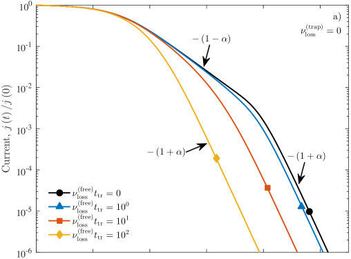
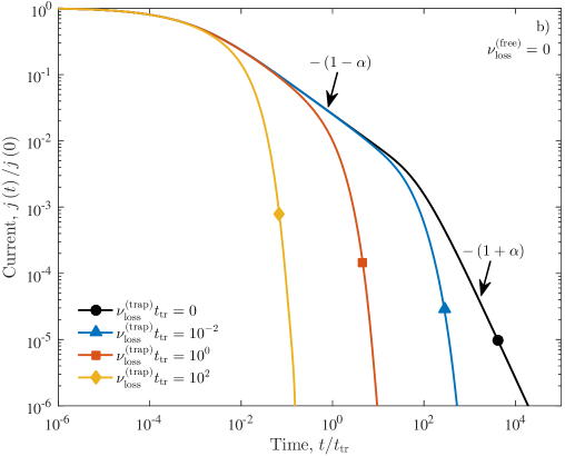
Figure 4: The impact of free and trapped particle recombination on current transients for an ideal time-of-flight experiment as modelled by Eq. (16) for the case of dispersive transport. Nondimensionalisation has been performed using the material thickness $L$, trap-free transit time, $t_{\mathrm{tr}}\equiv L/W$, and the initial current $j\left(0\right)=eN\left(0\right)/t_{\mathrm{tr}}$. For these plots we define the diffusion coefficient, $Dt_{\mathrm{tr}}/L^{2}=0.02$, the initial impulse location, $x_{0}/L=1/3$, and the trapping rate, $\nu_{\mathrm{trap}}t_{\mathrm{tr}}=10^{4}$. For dispersive transport to occur we have chosen to describe trapping times by the heavy-tailed distribution (112) with a trap severity of $\alpha=1/2$. This corresponds specifically to the distribution $\phi\left(t\right)=\frac{1}{2t}\left(\frac{\sqrt{\pi}}{2}\frac{\mathrm{erf}\sqrt{\nu_{0}t}}{\sqrt{\nu_{0}t}}-\mathrm{e}^{-\nu_{0}t}\right)$, where we have chosen $\nu_{\mathrm{0}}t_{\mathrm{tr}}=5\times 10^{5}$. The exponents of the power-law regimes are indicated with arrows. Such regimes, especially at late times, can be indicative of dispersive transport.

VII.2 Ratio of particle detrapping to trapping, $R$, for fractional transport

All of the results of the earlier sections depend in some way on the steady-state ratio between particles leaving and entering traps, $R$, defined explicitly in Eq. (32) or implicitly as given by the integral in Eq. (41). Unfortunately, the latter integral definition is not expected to converge when fractional transport is considered due to the asymptotic power law form (110) of the effective waiting time distribution. In this case, we have the alternative definition:

$$R\equiv 1+\frac{\Delta\nu_{\mathrm{loss}}}{\nu_{\mathrm{trap}}},$$ (113)

valid irrespective of the chosen heavy-tailed trapping time distribution. This definition provides an extension to the list of $R$ values in Appendix A of (Stokes et al., 2016) for fractional transport.

VII.3 Fractional Einstein relations

The generalised Einstein relation (105) for diffusivity in the direction of the field can be simplified when transport is fractional in nature. Here, as the mean trapping time diverges, the average time $\tau$ defined by Eq. (94) also diverges, resulting in the fractional Einstein relation

$$\frac{D_{\parallel}}{K}=\frac{k_{\mathrm{B}}T_{\parallel}+mW^{2}}{e}\left[1+\left(1+\Delta\right)\frac{\mathrm{d}\ln K}{\mathrm{d}\ln E}\right],$$ (114)

with

$$\Delta\equiv\frac{Q+\frac{3}{2}k_{\mathrm{B}}\left(T_{\mathrm{coll}}-T_{\mathrm{detrap}}\right)W\frac{\nu_{\mathrm{coll}}\left(\varepsilon\right)}{\nu_{\mathrm{eff}}\left(\varepsilon\right)}}{2k_{\mathrm{B}}T_{\parallel}W+2mW^{3}}.$$ (115)

This fractional Einstein relation is valid for any trapping time distribution with the asymptotic power law form of Eq. (110).

VIII Conclusion

We have explored a generalised phase-space model that considers collision, trapping, detrapping and recombination processes, all of which act selectively according to particle energy. We form balance equations (23)–(25) describing the conservation and transport of particle number, momentum and energy, and use these balance equations to form expressions for the particle mobility, Eqs. (43) and (53), and for the average particle energy in the form of Wannier energy relations (44) and (54). These Wannier energy relations were then used to provide conditions for particle heating or cooling due to collisions or trapping, Eq. (62), and recombination, Eqs. (74) and (78). Notably, recombination heating and cooling was found to occur even when particles recombined indiscriminate of energy, in contrast to the case where recombination occurs only in the delocalised states. Transport via combined localised/delocalised states was shown to produce negative differential conductivity under certain conditions (81), and the impact of scattering, trapping/detrapping and recombination on the anisotropic nature of diffusion was expressed through the development of the generalised Einstein relations (104) and (105). Lastly, fractional transport analogues of the aforementioned results were explored by using a trapping time distribution with a heavy tail of the form of Eq. (110).

For direct application of this model, it is necessary to have reasonable inputs for the trapping frequency, $\nu_{\mathrm{trap}}$, and the trapping time distribution, $\phi\left(t\right)$. Some progress has been made already for organic materials where the trapping time distribution can be calculated from the density of existing trapped states (Philippa et al., 2014). Also for dense gases/liquids, where trapped states are formed by the electron itself and the trapping time distribution is dependent on the scattering, fluctuation profiles and subsequent fluid bubble evolution (Cocks and White, 2016). Other investigations of trapping also exist in the literature (Ceperley and Alder, 1980; Miller and Reese, 2008; Cao and Berne, 1993), including free energy changes and solvation time scales, but none of these directly produces an energy-dependent trapping frequency or trapping time distribution. Presently, the focus of our attention is on the ab initio calculation of energy-dependent trapping frequencies and waiting time distributions in liquids and dense gases, as well as the simulation of charge carrier transport in 2D organic devices, including those with long-lived traps where transport is dispersive.

Appendix A Approximating higher order velocity moments

In Sec. V.1.2, we use first-order momentum transfer theory to obtain expressions for the drift velocity, Eq. (53), and mean energy, Eq. (54), of charged particles defined by the generalised Boltzmann equation (1). These velocity moments are each expressed in terms of the higher order velocity moments of energy flux $\boldsymbol{\xi}\equiv\left\langle\epsilon\mathbf{v}\right\rangle^{\left(0\right)}$ and mean squared energy $\left\langle\epsilon^{2}\right\rangle^{\left(0\right)}$. Here, we use zeroth-order momentum transfer theory to approximate these higher order moments by using the lower order ones.

In our previous work (Stokes et al., 2016), we consider constant process rates in the Boltzmann equation (1). This is functionally equivalent to the case of zeroth-order momentum transfer theory, as defined in Eq. (34). In Eq. (74) of (Stokes et al., 2016) we write the solution of the Boltzmann equation as a Chapman-Enskog expansion in Fourier-transformed velocity space. By considering the first term of this expansion, we find an approximation to the solution that is valid near the steady, spatially uniform state:

$$f\left(t,\mathbf{r},\mathbf{v}\right)\approx n\left(t,\mathbf{r}\right)\left[\omega_{\mathrm{coll}}\left(\varepsilon\right)\hat{w}\left(\alpha_{\mathrm{coll}},\mathbf{v}\right)+\omega_{\mathrm{trap}}\left(\varepsilon\right)\hat{w}\left(\alpha_{\mathrm{detrap}},\mathbf{v}\right)\right],$$ (116)

where the convex combination weights $\omega\left(\varepsilon\right)$ are defined in terms of collision and trapping frequencies by Eqs. (39) and (40). Here, the separate processes of collision scattering and detrapping have resulted in a solution containing non-Maxwellian velocity distributions of the form

$$\hat{w}\left(\alpha,\mathbf{v}\right)\equiv w\left(\alpha,v\right)\frac{\sqrt{\pi}}{\sqrt{2}\alpha W}\mathrm{erfcx}\left(\frac{1-\alpha\mathbf{v}\cdot\alpha\mathbf{W}}{\sqrt{2}\alpha W}\right),$$ (117)

where $w\left(\alpha,v\right)$ is the Maxwellian velocity distribution defined by Eq. (6), $\mathbf{W}$ is the drift velocity from zeroth-order momentum transfer theory, defined in Eq. (42), and the scaled complementary error function is defined as $\mathrm{erfcx}\left(z\right)\equiv\frac{2}{\sqrt{\pi}}\int_{z}^{\infty}\mathrm{d}\zeta\,\mathrm{e}^{z^{2}-\zeta^{2}}$.

As expected, taking velocity moments of this solution (116) reproduces the zeroth-order momentum transfer theory expressions for drift velocity $\mathbf{W}$, Eq. (43), and mean energy $\varepsilon$, Eq. (44). In the same vein, we can find approximations for higher order velocity moments written in terms of these lower order moments, $\mathbf{W}$ and $\varepsilon$. For energy flux we find

$$\boldsymbol{\xi}\approx\left(\frac{5}{3}\varepsilon+\frac{4}{3}mW^{2}\right)\mathbf{W},$$ (118)

and for mean squared energy:

$$\left\langle\epsilon^{2}\right\rangle^{\left(0\right)}\approx\frac{5}{3}\left[\omega_{\mathrm{coll}}\left(\varepsilon\right)\varepsilon_{\mathrm{coll}}^{2}+\omega_{\mathrm{trap}}\left(\varepsilon\right)\varepsilon_{\mathrm{detrap}}^{2}\right]+\frac{13}{3}\left(mW^{2}\right)^{2},$$ (119)

which is written in terms of the separate mean energies of $\tilde{w}\left(\alpha_{\mathrm{coll}},\mathbf{v}\right)$ and $\tilde{w}\left(\alpha_{\mathrm{detrap}},\mathbf{v}\right)$, given respectively:

$$\varepsilon_{\mathrm{coll}} \equiv \frac{3}{2}k_{\mathrm{B}}T_{\mathrm{coll}}+mW^{2},$$ (120)

$$\varepsilon_{\mathrm{detrap}} \equiv \frac{3}{2}k_{\mathrm{B}}T_{\mathrm{detrap}}+mW^{2}.$$ (121)