Statistical evolution of quiet-Sun small scale magnetic features using Sunrise observations

The evolution of small magnetic features in quiet regions of the Sun provides a unique window to probing solar magneto-convection. Here we analyze small scale magnetic features in the quiet Sun, using the high resolution, seeing-free observations from the Sunrise balloon borne solar observatory. Our aim is to understand the contribution of different physical processes, such as splitting, merging, emergence and cancellation of magnetic fields to the rearrangement, addition and removal of magnetic flux in the photosphere. We employ a statistical approach for the analysis and the evolution studies are carried out using a feature tracking technique. In this paper we provide a detailed description of the feature tracking algorithm that we have newly developed and we present the results of a statistical study of several physical quantities. The results on the fractions of the flux in the emergence, appearance, splitting, merging, disappearance and cancellation qualitatively agrees with other recent studies (see e.g., Lamb et al., 2008, 2013). To summarize, the total flux gained in unipolar appearance is an order of magnitude larger than the total flux gained in emergence. On the other hand, the bi-polar cancellation contributes nearly an equal amount to the loss of magnetic flux as unipolar disappearance. The total flux lost in cancellation is nearly $6-8$ times larger than the total flux gained in emergence. One big difference between our study and previous similar studies is that thanks to the higher spatial resolution of Sunrise we can track features with fluxes as low as $9\times 10^{14}$ Mx. This flux is nearly an order of magnitude lower than the smallest fluxes of the features tracked in the highest resolution previous studies based on Hinode data. The area and flux of the magnetic features follow power-law type distribution, while the lifetimes show either power-law or exponential type distribution depending on the exact definitions used to define various birth and death events. We also statistically determine the evolution of the flux within the features in the course of their lifetime, finding that this evolution depends very strongly on the birth and death process that the features undergo.

1 Introduction

The Sun’s magnetic field is to a large part concentrated into small-scale structures. This is particularly so in the quiet Sun. Although much is known about the structure of these features, there are still many unknowns (see e.g., de Wijn et al., 2009, for a review of quiet-Sun magnetism). Best studied are properties such as the field strength and the inclination angle of the field, although even for these widely different results have been published. The average magnetic field strength in network regions is known to be of on the order of $1-2$ kilo-Gauss (see e.g., Stenflo, 1973; Solanki & Stenflo, 1984; Rabin, 1992), but it is rather difficult to estimate inter-network quiet-Sun magnetic fields because different methods and different spectral lines have often provided discrepant results. For example, on the one hand, investigations using infrared (e.g., $1.5$ $\mu$m) lines give generally low field strengths below 600 G (see e.g., Lin, 1995; Solanki et al., 1996; Khomenko et al., 2003, 2005b), but with a tail of kG fields in the histogram of the field strengths shown by Khomenko et al. (2003). On the other hand, investigations using the visible line pairs (e.g., $525.0$ nm, $524.7$ nm, and $630.25$ nm, $630.15$ nm) have provided an inhomogeneous picture (see e.g., Socas-Navarro & Lites, 2004; Sánchez Almeida et al., 2003; Khomenko et al., 2005a; Orozco et al., 2007; Martínez González et al., 2008; Lagg et al., 2010), although in the recent studies the tendency has been towards a predominance of fields with low strengths (see, e.g. Asensio Ramos & Martínez González, 2014). The magnetic field inclination calculations differ in various studies and are also not well established yet. Investigations of Stokes profiles observed with Hinode/SP by Orozco et al. (2007) and Lites et al. (2008) suggest that the magnetic fields in internetwork regions are inclined predominantly horizontally with an average inclination angle of $20^{\circ}$ to the horizontal. However a study of bright points in Ca ii H images observed using SUNRISE/SuFI, which have a mean area close to $0.01$ Mm² (nearly $100$ times smaller than a typical granule), by Jafarzadeh et al. (2013) suggests that these magnetic elements in the internetwork regions are predominantly oriented vertically (Jafarzadeh et al., 2014b). For a comprehensive review on this topic we refer to Borrero et al. (2015, and the references cited therein).

The number of studies that have followed the evolution of individual features, or have followed a group of features through a certain phase of their evolution, is smaller. Such studies have mainly concentrated on individual phases in the lifetime of magnetic features, or particular dynamic processes, such as be the emergence of small loops (see e.g., Centeno et al., 2007; Martínez González et al., 2010; Guglielmino et al., 2012) and the linear polarization patches often associated with such emergence (Lites et al., 2008; Danilovic et al., 2010), the convective collapse of small-scale magnetic elements (see e.g., Nagata et al., 2008; Fischer et al., 2009), the evolution following the collapse (see e.g., Requerey et al., 2014, 2015; Utz et al., 2014), the evolution of the brightness (see e.g., Berger et al., 2007; Jafarzadeh et al., 2013), and motions of bright points (see e.g., de Wijn et al., 2008; Abramenko et al., 2011; Jafarzadeh et al., 2014a). Useful as they are, such studies cannot give a full picture of the evolution of magnetic features, since they do not attempt to give a complete statistical description.

A statistically more complete description has been attempted by a number of authors in recent years. Such studies have included not just the emergence, appearance, cancellation and disappearance of magnetic features, but have also taken into account the splitting and merging of the features, which are found to play an important role (see DeForest et al., 2007; Lamb et al., 2008, 2010; Parnell et al., 2009; Lamb et al., 2013; Iida et al., 2012; Gošić et al., 2014; Zhou et al., 2010, 2013; Iida et al., 2015, and the references cited therein). Such investigations have turned up some surprising results. Thus, only a small fraction of the magnetic flux in the quiet Sun is observed to emerge as bi-polar structures and just as small a fraction of flux is removed through cancellation of opposite polarity fields (see e.g., Lamb et al., 2013; Iida et al., 2015).

Such unexpected results demand a detailed analysis using an independent algorithm and the best data currently available. It is important to point out the contribution of the ground-based telescopes that provide high-spatial resolution data such as the NST of the Big Bear Solar Observatory (e.g., Goode et al., 2010) and the Swedish Solar Telescope of La Palma observatory (e.g., Scharmer et al., 2003). However, space or balloon-borne observatories have added advantages such as obtaining seeing-free observations, or of providing data at UV wavelengths that can be used to link the photosphere with higher layers and which are not possible from ground.

Here we present results obtained with a newly developed code that carefully classifies the features that participate in events such as simple appearance and disappearance, splitting, merging, bi-polar emergence and cancellation. The algorithm tracks the magnetic features by assigning a unique birth, unique death and a well defined lifetime to each of the detected magnetic feature. This code is applied to time series of high resolution magnetograms obtained in the quiet Sun with the Imaging Magnetograph eXperiment (IMaX, see Martínez Pillet et al., 2011) on the Sunrise balloon-borne telescope (see Solanki et al., 2010; Barthol et al., 2011). The earlier studies using high-resolution data to which our results can be compared have used Hinode/NFI data with a spatial resolution of 0″.3 ($6\times 10^{15}$ Mx, $6.5\times 10^{15}$ Mx and $5\times 10^{16}$ Mx being the lowest detected values of flux per feature reported by Zhou et al. 2013, Gošić et al. 2014 and Thornton & Parnell 2011, respectively). The higher spatial resolution (a factor of 5 per pixel, see Sect. 2) and the good polarimetric sensitivity of Sunrise/IMaX data means that we can detect and follow features with considerably lower flux ($9\times 10^{14}$ Mx is the lowest detected flux per feature) than previous investigations. The flux per feature is significantly larger than the often quoted flux per pixel because of the usually near-critical sampling of the diffraction limit of the telescope and the need to clearly distinguish features from noise. The fact that we can detect an order of magnitude lower flux than previous studies has the benefit that we can check if some of the seeming appearances and disappearances found in earlier studies are real or are only apparent due to limited sensitivity. We then carry out an analysis of the statistical properties of these features, such as distributions of area, magnetic field, magnetic fluxes, lifetimes and their relationships.

In Sect. 2 we briefly describe the observations. Sect. 3 is dedicated to a detailed description of the analysis procedure. In Sect. 4 we present a discussion of our statistical studies. Conclusions are drawn in Sect. 5 and details of the method are given in the two appendices.

2 The data

High spatial and temporal resolution data recorded by the Sunrise observatory (Solanki et al., 2010; Barthol et al., 2011; Berkefeld et al., 2011; Gandorfer et al., 2011; Martínez Pillet et al., 2011) on its first science flight in June 2009 provide us with an opportunity to derive the statistical properties and follow the evolution of quiet-Sun magnetic structures down to lower flux levels and at higher spatial resolution than previous studies.

A time series of forty two quiet Sun magnetograms observed with IMaX (Martínez Pillet et al., 2011) was considered. The spatial sampling is approx. $40$ km/pixel (with the spatial resolution being roughly $0.15-0.18$ arcsec) and the cadence is $33$ sec. Observations are available at four wavelength points within the spectral line Fe i at $525.02$ nm and at a wavelength in the nearby continuum $227$ mÅ  from the line core (V5/6 data). Four wavelength points sample the line at $\pm$ $40$ and $\pm$ $80$ mÅ  from the line center. We use phase diversity reconstructed data (see e.g., Gonsalves, 1982; Paxman et al., 1996; Vargas Domínguez, 2009) for descriptions of the technique and Martínez Pillet et al. (2011) for its application to Sunrise/IMaX data.

Figure 1: Left: Original $V/\bar{I}_{c}$ image at the middle of the time-series. Right: After applying the binary mask to the image on the left, as described in the main text.

We then consider the pixels in this set of images as the points in a cuboid. Two spatial co-ordinates ($x,y$) and a time co-ordinate ($t$) form the three dimensions of the cuboid. Application of phase diversity reconstruction to the data leads to the loss of $108$ pixels (Martínez Pillet et al., 2011). The features in the first and the last time steps are identified and tracked but not used for the statistics to avoid boundary errors in feature identification. The noise level of a single reconstructed IMaX image is $3\times 10^{-3}$ $I_{c}$, where $I_{c}$ is the continuum intensity. The effective size of usable image is $\sim 43\arcsec\times 43\arcsec$. Due to the low signal levels in Stokes $Q$ and $U$ (Danilovic et al., 2010) we concentrate on Stokes $I$ and $V$ in this paper.

At each time step, the spatially averaged continuum intensity $\bar{I}_{c}$ is used for the normalization of Stokes parameters $V$ and $I$ to obtain $V/\bar{I}_{c}$ and $I/\bar{I}_{c}$ at each wavelength. Then, the $V/\bar{I}_{c}$ data are averaged over the four wavelengths after reversing the sign of Stokes $V$ in the red wing of the line. We have excluded the continuum point for this averaging. We note here that we have used the wavelength averaged $V/\bar{I}_{c}$ only to identify the features as described in Sect. 3. This step does not affect the LOS magnetic field computation discussed in Sect. 3.2. The latter uses $V({\lambda})$ and $I(\lambda)$ individually at all wavelength points.

3 The analysis procedure

3.1 Identifying the magnetic features

A feature identification and tracking algorithm is necessary for studies of the evolution of magnetic features. A number of feature identification and tracking algorithms have been developed by several groups, a summary of which can be found in DeForest et al. (2007).

In this paper, a lane finding code originally developed for identifying granular structures (Hirzberger et al., 1999) is used to find all magnetic patches satisfying a set of predetermined criterion. This code has been extensively tested and applied to the study of supergranules by Hirzberger et al. (2008). The patches identified in this manner are then referred to as “features”. A feature is defined to be a collection of spatially connected pixels whose Stokes $V/I_{c}$ signal lies above a threshold of $3\times 10^{-3}$. This corresponds to two times the noise level, $\sigma$, of the data after the averaging over the 4 wavelength pixels in the line.

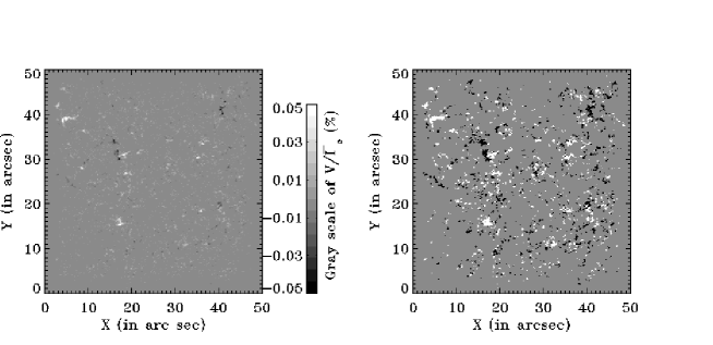
Since $2\sigma$ is a relatively low threshold, we, in addition, remove all features with an area less than 5 pixels. Further, the features touching the spatial boundaries at any time in the course of their evolution are also removed, since we only have a lower limit of their area and may be missing interactions with features outside the frame. We identify positive and negative polarity features separately. After the various steps described above, we obtain a total of 50255 features of both polarities, which were considered for the analysis. In Fig. 1 we display $V/\bar{I}_{c}$ image at the middle of the time series before (left panel) and after (right panel) identifying the features. Since we remove the features touching the spatial boundaries, we do not see features near the edge of the field-of-view. The code also checks if the features that are originally identified individually in different snapshots are the same underlying magnetic feature seen at two points in time. After that the binary masks of two consecutive time steps are compared with each other to see if a feature present in one mask is still present in the subsequent mask. In general, if two individually identified features in two consecutive time steps share at least one spatial pixel, then they are identified as the same feature at two different times. In practice, a number of other possibilities also occur. These are described in detail in Sect. 3.3.

3.2 Flux Computation

Using the center of gravity (COG) technique (see Rees & Semel, 1979), the strength of the line-of-sight (LOS) component of the magnetic field vector is determined from Stokes $V$ through the relationship

$$B_{\rm{LOS}}=|\Delta\lambda_{G}/C_{0}g\lambda_{0}^{2}|,$$ (1)

where $C_{0}=4.67\times 10^{-13}$m^-1 G^-1, $g$ is the Landé factor, $\lambda_{0}$ is the line center wavelength, and

$$\Delta\lambda_{G}=\frac{\int_{-\infty}^{+\infty}{V}\Delta\lambda d\Delta\lambda}{\int_{-\infty}^{+\infty}(I_{c}-I)\,\,d\Delta\lambda}.$$ (2)

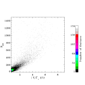
Here $I$ and $V$ represent the intensity and the circular polarization at a given wavelength, respectively, and $I_{c}$ the corresponding continuum intensity. The LOS magnetic field values $B_{\rm{LOS}}$ obtained when applying this technique to each pixel range between 0 to 2000 G. A SIR inversion sampling a region of the same data also provided kG fields (see Lagg et al., 2010; Requerey et al., 2014). We note here that these magnetic field values determined using the COG technique are averaged over the SUNRISE/IMaX spatial resolution element (i.e. no filling factor is introduced). A two-dimensional (2D) histogram of the number of features on the plane spanned by $B_{\rm{LOS}}$ and $|V/\bar{I}_{c}|$ is shown in Fig. 2. We use Equations (1 and 2) for computing the flux. However, since it is useful to show $|V/\bar{I}_{c}|$ on the horizontal axis of Fig. 2, we can trivially divide both numerator and denominator of Equation (2) by $\bar{I}_{c}$ (which is the continuum intensity averaged spatially over the entire image for each time frame). This step does not affect $B_{\rm{LOS}}$ values. It is cut-off at 1450 G due to the small number of pixels with large $B_{\rm{LOS}}$. Besides a significant scatter, the plot displays also a non-linear trend that is partly due to Zeeman saturation (Stenflo, 1973) and partly to temperature weakening of the spectral line (Zayer et al., 1990), although the latter effect is not as extreme as found in MHD simulations by Shelyag et al. (2007). Due to the influence of noise the $B_{\rm{LOS}}$ thus obtained cannot be trusted in pixels with low signal. Therefore in the following we determine and use a feature-averaged value, $\langle B_{\rm{LOS}}\rangle$, for computing the magnetic flux of a feature. The quantity $\langle B_{\rm{LOS}}\rangle$ is determined by averaging the Stokes $V$ data as discussed in the following paragraph. Here the angled brackets $\langle\,\,\,\rangle$ represent the value obtained from the spatial average of Stokes $V$ data over individual magnetic features.

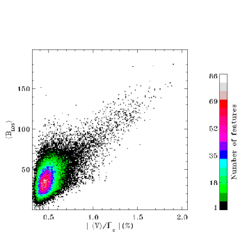
Thus, we compute the $\langle B_{\rm{LOS}}\rangle$ (Equations 1 and 2) using spatially averaged quantities $\langle V(\lambda)\rangle$, $\langle I(\lambda)\rangle$ and $\langle I_{c}(\lambda)\rangle$ within each of the 50255 identified magnetic features. A 2D histogram of the number of features on the plane spanned by $\langle B_{\rm{LOS}}\rangle$ and $|\langle V\rangle/\bar{I}_{c}|$ is shown in Fig. 3. The obtained averaged field values range between 0 and 100 G. Only 410 features out of 50255 features have field strengths between 100 and 200 G. The strong reduction in $B_{\rm{LOS}}$ values is caused by the inclusion of the weak signals at the edges of the magnetic features in the averaging. A higher threshold than the $2\sigma$ value that we have imposed leads to higher average $B_{\rm{LOS}}$ values as test calculations showed. However, since many features are then lost, we decided to maintain the lower threshold value. The thus obtained $\langle B_{\rm{LOS}}\rangle$ is then multiplied by the area covered by the feature to obtain its magnetic flux.

Figure 2: Magnetic flux computed using the COG technique. The figure shows a 2D histogram of the number of features on the plane spanned by $B_{\rm{LOS}}$ and $|V/\bar{I}_{c}|$ for each pixel.

Figure 3: Magnetic flux computed using the COG technique. A 2D histogram of the number of features on the plane spanned by the magnetic feature averaged LOS component of the field $\langle B_{\rm{LOS}}\rangle$ and the feature averaged unsigned Stokes $V$ normalized to the continuum intensity namely, $|\langle V/\bar{I}_{c}\rangle|$.

3.3 Definitions of features, parameters and events

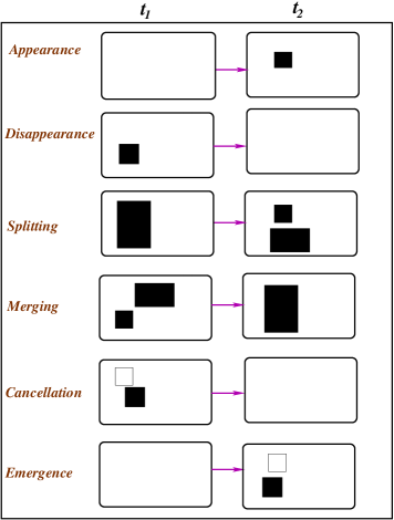
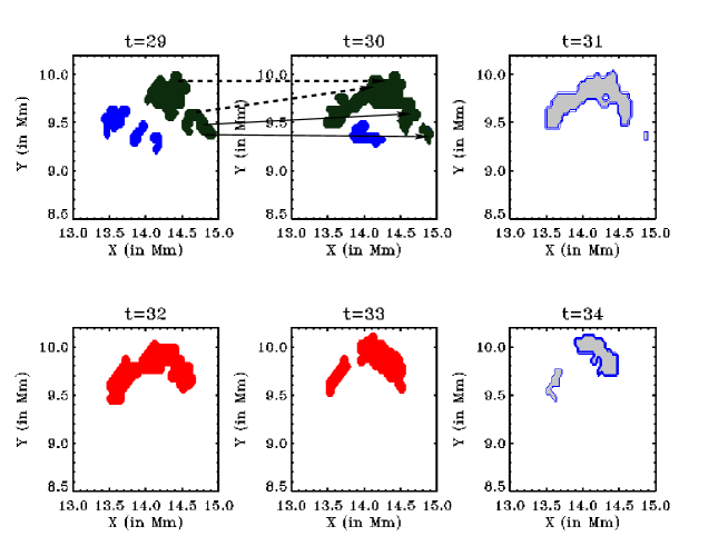
In this section we define and describe different terms, quantities and events on which our statistical study in this paper is based. The conventions defined here are used throughout this paper. Fig. 4 illustrates various possible interactions between the features, that are defined in this section.

Let us consider two successive time steps $t_{1}$ and $t_{2}=t_{1}+\Delta t$, where $\Delta t$ is the time step. From $t_{1}$ to $t_{2}$ important properties of a given feature that can change are, (1) spatial location of the feature, (2) shape and area of the feature, and (3) magnetic flux contained in that feature. In addition, the feature can disappear, or cancel with an opposite polarity feature, or merge with several same-polarity features, or split into multiple features between the times $t_{1}$ and $t_{2}$. Finally, the feature can appear or emerge (together with an opposite polarity feature) between the times $t_{1}$ and $t_{2}$. To quantitatively describe such evolutionary steps, several properties and events need to be defined.

$\bullet$ “Size” or “area” of a feature denoted as $A$, is given by the total number of pixels covered by a feature.

$\bullet$ Birth of a feature by appearance: If a feature appears at time $t_{2}$ at a given spatial location, but if the same spatial location at $t_{1}$ was empty (i.e. at $t_{1}$ no magnetic feature overlapped with any of the pixels occupied by the features at $t_{2}$), then we say that a feature is born by appearance at $t_{2}$.

$\bullet$ Death of a feature by disappearance: If a feature is present at $t_{1}$ at a given spatial location, but if the same spatial location at $t_{2}$ is found to be empty (i.e. at $t_{2}$ no magnetic feature overlaps with any of the pixels occupied by the features at $t_{1}$), then we say that the feature died or disappeared at $t_{1}$.

$\bullet$ Splitting of a feature: A feature at $t_{1}$ is said to split, if it breaks into two or more features at $t_{2}$. This is taken to happen when the features at $t_{2}$ (the children) have the same polarity as the parent, are spatially separated from each other and overlap with the parent by at least one pixel each. For the purposes of this paper we say that the parent feature died at $t_{1}$ due to splitting. At the same time, all the children at $t_{2}$ are considered to be newly born. An exception is made when the overwhelming part of the area or magnetic flux of the parent lives on in just one child, i.e. when only a small piece breaks off a much larger feature. Then the parent is assumed to live on as the biggest of the children. All other children are assumed to be newly born. This is described more quantitatively under ‘area-ratio criterion’ below. In Fig. 5 examples of splitting events are shown in red.

$\bullet$ Merging of features : Merging is said to have taken place if two or more features of the same polarity at $t_{1}$ combine into a single feature of the same polarity at $t_{2}$, and the child overlaps spatially by at least one pixel with each of the parent features. For the purposes of this paper we say that all parent features died at $t_{1}$ due to merging and a new feature is born at $t_{2}$. Again, an exception is made if one parent is overwhelmingly larger than the other(s). In Fig. 5 examples of merging events are shown in blue.

$\bullet$ To rule out that a feature is pronounced dead just because a tiny part of it breaks off, or because it merges with a much smaller feature, the areas of involved features at a given time step are compared. We compare areas of child features for a splitting event and areas of parent features for a merging event. If the largest feature is more than a predetermined factor times bigger than the second largest, then this feature is assumed to be a continuation of the parent (in the case of splitting) or to continue as the child (in the case of merging). All other children are classified to be born due to splitting-off birth events. To test how strong the effect of the above area-ratio is, we consider the following set of area-ratios: 2:1, 3:1, 5:1 and 10:1. For example, in a 2:1 area ratio criterion for a splitting event, the parent is considered dead only if the area of the largest child is less than twice the area of second largest child. A quantitative description of splitting and merging events is given in Appendix A.

The area-ratio criterion also helps to bring order to complex events, where splitting and merging may be taking place at the same time. An illustration of this is shown in Fig. 5. Let us focus on the first two panels (first row from left to right). The four features involved in a complex event are the filled green features connected by arrows (see figure caption). In principle, since there are two features at both time steps one could say that no interaction has taken place. However, one of these features has grown considerably, while the other has shrunk. In addition, one of the features at $t_{1}=29$ overlaps with two features at $t_{2}=30$ and vice versa. Such a situation could be the result of a combination of a splitting event plus a merging, both taking place within a single time-step, but it can also be produced by other combinations of events. The chosen area-ratio criterion along with a set of priority criteria described in Appendix B to eliminate the ambiguity (see next paragraph) leads to one such combination being preferred. After applying an area-ratio criterion of 5:1 and the priority criterion to eliminate ambiguity the splitting event is discarded, the merging event is retained, and the remaining small green feature in the second panel is considered to be newly born by a splitting-off birth event. A blue filled feature in panel 2 of Fig. 5 dies by disappearance and the other two filled green features continue to live as gray filled features in panel 3. The smaller gray filled feature in panel 3 disappears and the larger gray feature continues to live as the only red filled feature in panel 4. This eventually splits into two red filled features in panel 5, both of which continue to live as gray filled features in panel 6.

$\bullet$ Simultaneous events and ambiguities: Statistically, it is not so rare for splitting and merging events to happen simultaneously. An example of a possible simultaneous splitting and merging event was discussed in the previous paragraph (filled green features in first two panels of Fig. 5). The events are marked by arrows (see figure caption). Therefore, additional care must be taken to handle such cases. In Appendix B we describe in detail all possible simultaneous events and how we handle them. Eventually based on a set of rules all the ambiguities in simultaneous events are eliminated and are classified into different birth and death cases defined above.

$\bullet$ The lifetime of a feature is defined to be the interval of time between the birth of a feature (either through appearance, emergence, or from splitting or merging) and its death (through disappearance, cancellation, splitting or merging).

$\bullet$ Emergence events are composed of the appearance of opposite polarity features close in space and time. First, a spatial overlap (after dilation, see Appendix C) of one or more positive features with one or more negative features are detected. Then we apply a flux-ratio criterion between the sets of positive and negative features. We consider four cases, namely, 10:1, 5:1, 3:1 and 2:1. If the ratio of sum of the fluxes of the interacting positive polarity features to that in the interacting negative polarity features satisfies the imposed flux-ratio criterion, then it is identified as an emergence event. We describe what we mean by “close in space and time” in Appendix A. We classify the emergence into two types: (a) Time-symmetric and (b) Time-asymmetric bi-polar emergence.

(a) Time-symmetric emergence: The spatially close (neighboring) opposite polarity features appear at the same time step. In this case, the total flux contained in the emergence event is $F_{\rm{SYM,EM}}=2\,\,{\textrm{min}}(F_{+},F_{-})$, where $F_{+}$ is the total flux of the set of positive features emerged and, $F_{-}$, that of the negative features emerged.

(b) Time-asymmetric emergence: The opposite polarity features appear spatially close to each other at a given time-step, but the time frames at which the opposite polarity features are born, are offset by one or more steps. Here, only features of one of the polarities are newly visible near a set of close-by opposite polarity features that already exist. The already existing features could have been born in any of the previous time steps. In this case, the total flux contained in the emergence event is $F_{\rm{ASYM,EM}}=2\,\,F_{+}$ if the newly emerged features are positive and $F_{\rm{ASYM,EM}}=2\,\,F_{-}$ if the newly emerged features are negative. We have implicitly assumed that a bi-polar feature has emerged, but that one polarity appears within a patch of pre-existing field.

We note here that although we have defined time-asymmetric emergence events such that the time-separation between the already existing features and newly emerged features is one or more, for most of the cases, the time-separation is small. For e.g. for the 10-1 area-ratio criteria, the maximum time-separation between the opposite polarity features in time-asymmetric emergence is $\sim$ 9 minutes. However, the number of features having a time-separation greater than 5 minutes is only 4 and that greater than 2 minutes is only 10 % of the total number of features appearing as already existing time-asymmetric counterparts.

$\bullet$ Cancellation events occur when two or more neighboring opposite polarity features at time step $t_{1}$ exhibit a spatial overlap (after dilation, see Appendix C) in such a way that in the subsequent time step $t_{2}$ the sum of the fluxes of these features has decreased by a significant amount, where “significant” is decided by the rule,

$$\Sigma_{i=1}^{N_{1}}|f_{i}|-\Sigma_{i=1}^{N_{2}}|f_{i}|\geq N_{c}\sqrt{\Sigma_{i=1}^{N_{1}}{\sigma_{f_{i}}}^{2}},$$ (3)

where $f_{i}$ is the magnetic flux of the $i$-th feature, $\sigma_{f_{i}}$ is the noise level in the flux of the $i$-th feature, $N_{1}$ is the number of features involved in a cancellation event at time step $t_{1}$, $N_{2}$ is the number of features involved in the same cancellation event at time step $t_{2}$ and $N_{c}$ is an arbitrary factor (here we chose $N_{c}$=5).

We have three types of cancellation events.

(a) Complete cancellation: If at any time step $t_{1}$, a spatial overlap (after dilation, see Appendix C) of two sets of opposite polarity features leads to disappearance of both sets of features, then it is marked as a complete cancellation event.

(b) Semi cancellation : If at any time step $t_{1}$, a spatial overlap (after dilation, see Appendix C) of two sets of opposite polarity features is found to satisfy the condition for cancellation (see above) according to Equation (3), leading to disappearance of features of only one polarity, then the event is considered to be a semi cancellation event.

(c) Partial cancellation : If at time step $t_{1}$, a spatial overlap (after dilation, see Appendix C) of two sets of opposite polarity features is found to satisfy the condition for cancellation (see above) as described in Equation (3), leading to survival of both the polarity features, then the event is identified as a partial cancellation event.

$\bullet$ Instantaneous (magnetic) flux of a feature: The flux of a feature at a given time step. The instantaneous flux of a feature in a birth event (death event) is the flux that it carries at the time step of its birth (death).

$\bullet$ Maximum (magnetic) flux of a feature: The maximum value of flux of a feature attained during the course of the feature’s lifetime.

$\bullet$ Total instantaneous (magnetic) flux in a birth or a death event: The sum of the fluxes of all those features in the entire considered data set, which are born by a particular birth type or died by a particular death type at the time of birth or time of death (sum of instantaneous fluxes).

$\bullet$ Total maximum (magnetic) flux in a birth or a death event: The sum of the maximum fluxes of all those features in the entire data set, which are born by a particular birth type or died by a particular death type.

$\bullet$ Total (magnetic) flux (in emergence or cancellation): The sum of the (instantaneous or maximum) fluxes of those features in the time series, that participate in emergence or cancellation. Here the total flux in emergence includes not just the flux of features that are born by emergence, but the total flux emerged, which is $\Sigma F_{\rm{SYM,EM}}+F_{\rm{ASYM,EM}}$, with $F_{\rm{SYM,EM}}$ and $F_{\rm{ASYM,EM}}$ defined above. Similarly the total flux in cancellation not only includes the flux lost in features that die by cancellation, but also includes the flux lost in surviving features in semi and partial cancellation.

$\bullet$ Total (magnetic) flux (in all the birth events): The sum of the (instantaneous or maximum) fluxes of those features in the time series, that are born in all considered birth events. In case of total instantaneous flux, it is the sum of the fluxes at the time of birth.

$\bullet$ Total (magnetic) flux (in all the death events): The sum of the (instantaneous or maximum) fluxes of those features in the time series, that died from all considered death events. In the case of the total instantaneous flux, it is the sum of fluxes at the time of death.

Figure 4: Illustration of various possible interactions between the magnetic features. Only the simplest possibilities are shown in this diagram. Black and white refer to magnetic features with opposite polarities from each other. A more detailed description of all possible events is provided in the main text.

Figure 5: Illustrative example of evolution of a group of magnetic features over 6 time steps. All magnetic features in this frame have the same polarity. Features involved in merging and splitting events are indicated by filled colored contours. The arrows in the first two panels refer to a particular event involving simultaneous splitting and merging, as discussed in the main text. The dashed arrows indicate the merging event while solid line arrows mark the splitting event. The features that are involved in this event in the first 2 panels are colored blue and green. The features that do not split or merge in the plotted frame are shaded gray. The order of time steps proceeds row by row, and from left to right in each row.

Figure 6: Histograms of magnetic-feature averaged value of $|V/\bar{I}_{c}|$ (panel a) and maximum value of $|V/\bar{I}_{c}|$ per feature (panel b). Red lines are fitted power-law curves to these histograms (see text).

4 Results and discussion

4.1 The distributions of average and maximum value of $|V/\bar{I}_{c}|$

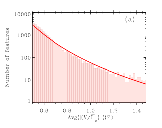
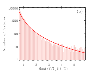
In Fig. 6 we plot histograms of average and maximum of the $|V/\bar{I}_{c}|$ within each feature. Note that smaller values are probably affected by the noise, and the finite spatial resolution. The average $|V/\bar{I}_{c}|$ distribution has mean and median values of $0.51$ % and $0.48$ % respectively, and the maximum $|V/\bar{I}_{c}|$ has mean and median values of $0.82$ % and $0.69$ % respectively. The average and maximum values of $|V/\bar{I}_{c}|$ follow power-law distributions with power law indices $-4.6$ and $-3.3$ respectively. These indices are much larger than those found for the magnetic flux per feature (see Sect. 4.2; Parnell et al., 2009; Buehler et al., 2013).

Figure 7: Histograms of areas (panel a) and feature-averaged LOS magnetic field values (panel b) in the features. Red lines indicate a power-law fit in panel (a) and a normal distribution in panel (b).

Figure 8: Histograms of instantaneous (panel a) and maximum (panel b) fluxes of the features. Red lines indicate power-law fits.

Figure 9: Histograms of instantaneous (panel a) and maximum (panel b) of the fluxes of the features, with bins equi-distant in log(flux). Colored lines indicate power-law fits with different minimum fluxes given in table 1.

4.2 Distribution of the area, magnetic field and magnetic flux of the features

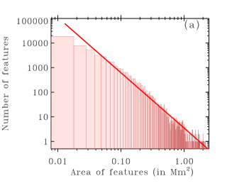
In Fig. 7(a) we plot the histogram of magnetic feature area. The areas of the features range from a minimum of $\sim 7.8\times 10^{-3}$ Mm² (or 5 pixels, which is the lower limit we have set for features selected for investigation) to a maximum of $\sim$ 2.5 Mm² ($1585$ pixels). The areas of the magnetic features closely follow a power law distribution of the form $a\,x^{b}$ with index $b=-2.25$. It closely matches with the power law index of $-2.2$ obtained by other recent studies using Hinode/SP data for such area distributions (see Buehler et al., 2013, and the references cited therein).

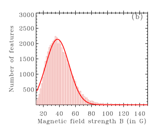
A histogram of the feature-averaged LOS magnetic field component, determined using the COG technique (see section 3.2 for details), is displayed in Fig. 7(b). The magnetic field values thus obtained are weak, as expected from Fig. 3, and the distribution is surprisingly symmetric, although with a tail towards stronger fields. The mean and median values are $41$ G and $39$ G respectively. The feature-averaged magnetic field strength values range between $11$ G to $198$ G. These values are somewhat lower than expected for an equipartition field (200-400 G, e.g., Solanki et al., 1996). The field strength values nearly follow a normal distribution.

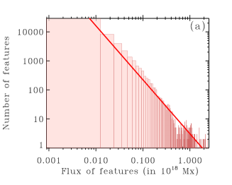
In Fig. 8(a) we plot the histograms of the instantaneous fluxes of the magnetic features. Here we consider all the 50255 features in the time series, i.e. considering all the features that represent evolution/history of a given feature in different time steps, to be independent. The minimum and maximum of the distribution is $9\times 10^{14}$ Mx and $2.5\times 10^{18}$ Mx respectively. The fluxes follow a power law distribution of the form $a\,x^{b}$ with index $b=-1.85$ which is consistent with Parnell et al. (2009). Other recent studies using Hinode data also obtain a power law index close to $-1.8$ (see e.g., Iida et al., 2012; Buehler et al., 2013, the focus of the former being the network fields).

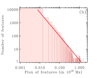
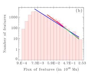
In Fig. 8(b) we plot histograms of maximum fluxes of the magnetic features. Here maximum flux of a feature refers to the maximum of the feature’s magnetic flux during it’s entire lifetime (see Sect. 3.3), with lifetime being obtained for the 10:1 area-ratio criterion. The maximum fluxes also follow a power-law distribution with power-law index $b=-1.78$. The power-law index for maximum fluxes is close to that obtained for instantaneous fluxes as are the minimum and maximum flux values. The fit parameters are listed in Table 1.

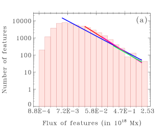
However, the tail region of the histogram suffers from very poor statistics in Fig. 8 leading to seeming gaps in the flux per feature. To avoid these holes, we plotted the histograms with bins of equal width in logarithm of the fluxes in Fig. 9. Power-law fits to the histograms of the fluxes depend sensitively on the smallest flux per feature in the distribution (see also Parnell et al., 2009; Iida et al., 2012). We show power-law fits of these histograms for four different smallest flux per feature values. The fit parameters of these distributions, and the corresponding $\chi^{2}$ values are listed in Table 1. We note here that the value $2\times 10^{17}$ Mx for the smallest flux per feature, chosen for the green power law fit in Fig. 8 is same as that in Parnell et al. (2009) for the Hinode data. In the remaining cases, the two extreme smallest flux per feature, either try to fit numbers of features that are clearly affected by instrumental resolution and sensitivity, or affected by the small number of points it is fitting. However, they give an indication of the uncertainty of the power-law index to the choice of smallest flux per feature. Therefore, the fit with smallest flux per feature of $10^{16}$ Mx appears to provide the most reasonable fit among the four cases. Clearly, the power-law index depends strongly on the type of binning, with all the fits to the bins of equal size on a logarithmic scale giving far lower power-law indices than those to the bins of equal size in linear scale. To our knowledge this dependence has not been previously highlighted and the type of binning is often not discussed carefully in studies of magnetic flux distribution. There is a need to investigate these effects thoroughly, as having bins that are equally broad on a logarithmic scale returns power-law fits that are not consistent with the results of Parnell et al. (2009). At present it is unclear, which type of binning provides the better description. However, a study of the best type of binning is outside the scope of this paper.

The feature-averaged field strength values shown in this paper are much smaller compared to the field strengths of quiet Sun features found by Khomenko et al. (2003); Lagg et al. (2010) and Riethmüller et al. (2014). The main reason for this discrepancy is that we show feature-averaged values. Also, we determined only the LOS component of the field and, unlike the latter two groups of authors cited above, consider all magnetic features visible in Stokes $V$ and not just those that are associated with bright points. In Fig. 2 we have shown the flux of individual pixels where the $B_{\textrm{LOS}}$ reach kG values.

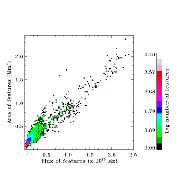
In Fig. 10 we present a 2D histogram of the number of features on the plane spanned by the magnetic flux $\Phi$ in the features and their areas $A$. This figure shows that area and fluxes are almost linearly related. This linear behavior is useful because it implies that we can constrain the classification of birth and death events, either through an area-ratio criterion or through a flux ratio criterion according to convenience.

Figure 10: 2D histogram of the number of features on the plane spanned by the magnetic flux $\Phi$ in the features and their areas $A$.

4.3 Birth and death of magnetic features

In this section we discuss statistics of the births and deaths of magnetic features. We start by considering only interactions between features of the same polarity in Sect. 4.3.1. Later, in Sect. 4.3.2 we include also interactions between magnetic features of opposite polarity.

4.3.1 Unipolar interactions

In Table 2 we present the number and percentage of features that are born or die according to different processes. The numbers are given for four different area-ratio criteria (see Sect. 3.3 for details). For the 10:1 area-ratio criterion, a total of 18037 features were born in the course of 40 time steps (i.e. over the entire considered time series), while $17779$ features died. The difference between the births and deaths is explained by the fact that whereas $1019$ features were present in the first frame, $1277$ were there in the last. As we decrease the area-ratio criterion, from 10:1 to 2:1, i.e. tighten the requirement for a merging or splitting event to result in a birth or death, the number of features that are born is reduced to $15124$ and those that die to $14866$. We have splitting-off birth and merging-into death processes resulting from those features which do not satisfy the area-ratio criterion in splitting and merging (see Sect. 3.3 for details). They form a significant fraction of features that are born or have died. As expected, this number becomes largest for the extreme area-ratio criterion of 2:1.

Among the other types of unipolar birth events, most features are born due to appearance, followed by splitting, and then by merging. Not surprisingly, the number of features born due to splitting is more than twice that from merging, since splitting gives rise to the birth of two or more features whereas merging leads to the birth of only one feature. With a decrease in the area-ratio criterion, the number of features born by splitting and merging decreases, those born by splitting-off birth events increases, since the features that would otherwise result from splitting and merging are now considered to be simply born by splitting-off birth events. Similarly, among the unipolar death events, death due to disappearance is the most common among processes responsible for the death of magnetic features, followed by merging and then by splitting. For the same reason that there are nearly twice as many births by splitting as by merging, there are nearly twice as many deaths by merging than by splitting.

In Table 3 we list the total instantaneous magnetic flux of the features in various birth and death events (see Sect. 3.3). About $3.6\times 10^{18}$ Mx of flux is present at the beginning of the time-series and nearly the same amount of flux ($4.0\times 10^{18}$ Mx) exists at the end of the time-series. The amount of flux is distributed differently between the various birth processes than just the number of events. E.g., for the area-ratio criterion of 10:1, although nearly half of the features are born by appearance, this process contributes only $12$ % to the total flux in newborn features. This suggests that mainly small features are born by appearance which is confirmed by considering the flux per feature also listed in Table 3. Splitting and merging events, respectively, provide $44.5$ % and $41.5$ % of the total flux of new features (although not new flux at the solar surface, since fresh flux is provided only by appearance and emergence events). The percentage of the flux in appearance events increases as the area-ratio criterion is tightened (i.e. the ratio made smaller) and reaches $27$ % of the total instantaneous flux for the 2:1 area-ratio case. The flux contained in splitting-off birth events are as small as $1.5$ % for an area-ratio of 10:1, which increases with a decrease in the area-ratio and reaches $14.6$ % for the 2:1 case. A similar behavior is observed in death events.

In Table 4 we provide the total maximum flux distribution in various birth and death events (see Sect. 3.3). The total maximum flux has a slightly different distribution than the total instantaneous flux in different birth and death events. As discussed above, the total instantaneous flux distribution in birth events shows that features born by appearance have lower values of flux on average. Whereas, the maximum flux in a feature born by appearance reached in the course of its life is roughly a factor of nearly $1.5-1.6$ larger than its flux at birth (see also Gošić et al., 2016). Consequently, features born by appearance events display a larger relative contribution to the total flux when the maximum flux is counted. Conversely, the contribution of features born by splitting and merging to the total maximum flux is smaller than their contribution to the total instantaneous flux. A similar behavior is observed in death events.

4.3.2 Interactions between features with opposite polarity

In this section we investigate the contribution to the total flux from emergence and cancellation of bi-polar magnetic features. In the case of emergence, we consider different flux-ratio criteria such that only those events are considered to be bi-polar emergences in which the ratio of fluxes between the involved opposite polarity features is smaller than the imposed ratio. Here we consider the ratios 10:1, 5:1, 3:1 and 2:1. However, since flux and area are linearly related (see Fig. 10), hereafter, to avoid confusion in discussions, we use the term “area-ratio criterion” in place of flux-ratio criterion. We do not consider any flux-ratio criterion for cancellation events, i.e. the flux in the two sets of the two opposite polarity features involved in the cancellation can be arbitrarily different, thus allowing for partial cancellation (see definition of cancellation events in Sect. 3.3).

Table 2 reveals that only $1-2$ % of the features in the considered data set are born through bi-polar emergence, and at the time of birth these features carry only $0.3-0.5$ % of the total instantaneous magnetic flux in the birth events. When we consider total maximum magnetic flux in birth events, they contribute between $0.5-1.0$ %. Thus emerging features grow to reach $1.7-2$ times their flux at birth. We note here that, the fluxes given here and in Tables 3 and 4 correspond to the fluxes of the features that are born due to emergence. I.e. these include the fluxes of the features with both polarities in time-symmetric emergence events, as well as the fluxes of the newly emerged features in time-asymmetric emergence events (but not the fluxes of the already existing opposite-polarity features, since these are not newly born features). The total emerged flux in all the emergence events, namely, $\Sigma(F_{\rm{SYM,EM}}+F_{\rm{ASYM,EM}})$ (as defined in Sect. 3.3) is higher than these values, in both, instantaneous and maximum flux. Since the asymmetric emergence dominates over symmetric emergence, the total flux that emerged is nearly twice the total flux of the features that are born due to emergence. For the 10:1 area-ratio criterion, a total of $3.9\times 10^{18}$ Mx instantaneous flux and $9\times 10^{18}$ Mx maximum flux is gained in emergence. Even then the total flux in emergence events is an order of magnitude smaller compared to the total flux detected in appearances. Hence either bi-polar emergence events are difficult to detect in the quiet Sun, or these events are comparatively rare.

On the other hand we see nearly $8.7-10.4$ % of the features dying due to cancellation. The total instantaneous flux lost in cancellation events ranges between $1.7$ % and $3.6$ % of the total flux lost in death events. When we consider total maximum flux, it ranges between $2.9$ % and $5.6$ %. We note that the fluxes ascribed to cancelling events given here and in Tables 3 and 4 correspond only to the fluxes of the features which undergo cancellation and die. I.e. the fluxes lost from the interacting features in semi and partial cancellation events which survive in the next time step, are not included here. This is because here we are interested in the fluxes that account for death of the features. The total flux lost in complete, semi and partial cancellation events (i.e. the sum of fluxes lost in died and surviving features) is nearly four times the total flux in the features that die due to complete, semi and partial cancellation. This accounts for $7$ % of the total instantaneous flux and $11$ % of the total maximum flux loss in cancellation for the 10:1 area-ratio criterion. In this case, a total of $3.1\times 10^{19}$ Mx instantaneous flux and $5.3\times 10^{19}$ Mx maximum flux is lost. A smaller number of cancelling features contributing more flux loss suggests that the features undergoing cancellation are on average large. However, these large cancelling features are the features that survive after semi and partial cancellation because cancelling features that disappear are small and carry low flux (see discussions in Sect. 4.6). The total instantaneous flux (total maximum flux) that is lost in the cancellation is nearly $8$ times ($6$ times) larger than the total flux gained in emergence for the 10:1 area-ratio criterion. Also, a roughly equal amount of flux is removed from the magnetograms (and possibly from the solar surface) by cancellation as by disappearance.

In Table 5 we list the flux distributions in time-symmetric and time-asymmetric emergence events with respect to the total flux in emergence events (not with respect to the total flux in all the birth events), as well as in complete, semi and partial cancellations with respect to only the total flux lost in cancellation. For example, in the case of 10:1 area-ratio criterion, the fractions of the total emerged instantaneous flux of $3.9\times 10^{18}$ Mx in time-symmetric and time-asymmetric emergence events is listed in the 3rd and 4th rows of Table 5. It is interesting to note that, among the captured bi-polar interactions, $80-90$ % of the features emerged in time-asymmetric emergence events. The time-symmetric emergence events corresponds to only $3-10$ %, ($4-14$ %) of the total instantaneous (total maximum) flux added by bi-polar emergence, so that time-asymmetric emergence events dominate. In cancellation events, complete cancellation corresponds to only $2$ % ($3$ %) of the total instantaneous (total maximum) flux that is lost in cancellations while semi and partial cancellation events account for the rest.

4.4 Discussion

A similar study as described in Sect. 4.3 has been carried out by Lamb et al. (2008) based on SOHO MDI magnetograph data, and by Zhou et al. (2010); Wang et al. (2012); Lamb et al. (2013); Gošić et al. (2014, 2016) based on Hinode/SOT/NFI data. Their approach differs somewhat from ours in the definition of the events and the type of data used and partly also in the aims of the studies. Thus, our data have higher spatial resolution, so that we see smaller features. Also, these authors did not introduce a threshold for merging and splitting events. A comparison can still be useful, however, although it only makes sense to compare the statistics obtained with 10:1 area-ratio criterion. In the following we provide a detailed comparison of our results with those by Lamb et al. (2008, 2013).

The following discussion is summarized in Table 6.

(1) The appearances account for $12$ % of the total flux found by Lamb et al. (2008). The flux contained in appearance in the present work accounts for $12$ % of the total instantaneous flux and $19.1$ % of the total maximum flux for area-ratio criterion 10:1. Since their fluxes correspond to the maximum flux, this shows that we obtain more total flux in appearance events than they find.

(2) The ‘fragmentation’ birth type in Lamb et al. (2008) gives rise to $76$ % of the total flux in newborn features, whereas we find $44.5$ % and $41.5$ % of total instantaneous flux and $41.8$ % and $36.5$ % of total maximum flux in splitting and merging birth events, respectively, giving a total of $80$ %. The small difference between the two results is partly due to differences in the details of the definitions.

(3) Emergence accounts for nearly $1$ % of the total flux in Lamb et al. (2008). We have $0.5$ % of total instantaneous flux, and $1$ % of total maximum flux in the features that are born by emergence. However, as discussed earlier, the actual total flux emerged is twice the total flux appeared in features born by emergence. Therefore the total flux appearing through emergence accounts for $1-2$ % of the total flux in birth events, still in agreement with the result of Lamb et al. (2008).

(4) When we focus only on the new flux at the solar surface, which means the total flux gained through appearance and emergence events, (i.e. excluding the total fluxes in the features born by splitting and merging events, which is not new at the solar surface), appearance accounts for $92.4$ % of the total instantaneous flux, and $91$ % of the total maximum flux, so that the new flux in bipolar emergence events accounts for less than $10$ % of the new flux at the solar surface, at least at the sensitivity and resolution of the Sunrise/IMaX instrument. In this point we assume that, the term ‘total instantaneous/maximum flux’ corresponds to the sum of the total instantaneous/maximum fluxes in all appearance and emergence events.

(5) Lamb et al. (2008) could not assign $10.9$ % of the birth events to a clear category (they referred to these as error events), while we uniquely assigned a birth or death category to every feature as described in Section 3.3 and Appendix B. This accounts for some of the differences in the results.

(6) Uni-polar death types (disappearance, splitting and merging) are found to have similar statistics as birth types, in agreement with the findings of Lamb et al. (2008).

(7) In the analysis by Lamb et al. (2013), where the authors focus only on disappearance and cancellation, nearly $83$ % of the total flux is removed from the visible features by disappearance. In our case, if we estimate the percentage of flux lost in disappearance and cancellation by considering only these two types of events, disappearances accounts for $59$ % of the total instantaneous flux, and $60$ % of the total maximum flux. However in the above estimation if we further leave out also the fluxes lost in the features that survive in semi and partial cancellation to consider only the fluxes lost in features that die by disappearance and cancellation (as done by Lamb et al., 2013) then disappearance accounts for $86$ % of the total instantaneous flux, and $85$ % of the total maximum flux, in good agreement with the results of Lamb et al. (2013). Here and in the next paragraph again, we assume that, the term ‘total instantaneous/maximum flux’ corresponds to the sum of instantaneous/maximum fluxes in those events considered in the context.

(8) Cancellation in Lamb et al. (2013) accounts for $12$ % of the total flux. If we leave out the fluxes contained in surviving features in semi and partial cancellation (as done in Lamb et al., 2013), we obtain $14$ % total instantaneous flux and $15$ % total maximum flux that corresponds to cancellation event, which is comparable to the results obtained by Lamb et al. (2013).

4.5 Lifetimes of the features

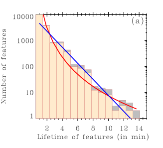
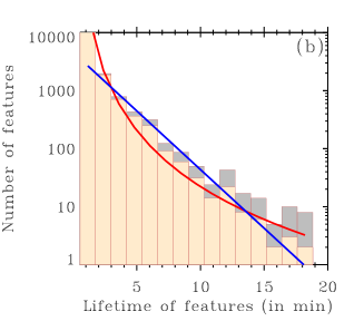
In Fig. 11 we plot histograms of lifetimes of the features, where the lifetime is determined as described in Section 3.3. A correction factor was proposed by Danilovic et al. (2010) to avoid underestimating the lifetimes for the same observations, as the duration of the time-series is itself comparable to the lifetimes of longer-lived features. The suggested weight to be multiplied to each bin of the lifetime distribution is $(n-2)/(n-1-m)$, where $m$ is the number of frames a feature lives, and $n$ is the total number of frames. We show lifetime histograms before (yellow-shaded) and after (gray-shaded) applying the correction factor. The plotted histograms are for the two extreme ratios of the areas of the children/parents, 10:1 and 2:1 respectively. Nearly $39$ % and $36$ % of the features for the 10:1 and 2:1 cases respectively, in the lifetime histograms live for just one time step. The more restrictive the area-ratio criterion restricting the death of features, the larger the number of long lived features, since a higher number of splitting and merging events are not counted as contributing to the birth or death of the larger feature (although for the smaller features they are involved in these events).

The mean and median lifetimes are $1.4$ and $1.1$ minutes ($85$ and $66$ seconds) respectively for the 10:1 case and are $1.6$ and $1.1$ minutes ($96$ and $66$ seconds) respectively for the 2:1 case. Similar lifetimes were also reported by Zhou et al. (2010). These small mean and median lifetimes are clearly dominated by the large number of features that live for just one time step. Thus, the mean lifetimes we find are much shorter than the lifetimes of the bright points found by Jafarzadeh et al. (2013) using the same Sunrise data set.

We fitted an exponential distribution of the form $N(\tau)=a\,e^{b\tau}$ and a power law distribution of the form $N(\tau)=a\,b^{\tau}$ to the lifetime histograms, where $N(\tau)$ is the number of events with a lifetime between $\tau$ and $\tau+\delta\tau$. In the case of the exponential distribution we refer to the parameter $b$ as the ‘exponential fit index’ and in the case of the power-law distribution we refer to $b$ as the ‘power-law index’. The fit parameters for the two types of distributions are tabulated in Table 7. It reveals that the $\chi^{2}$ of the fit is smaller for the exponential distribution in the 10:1 case than that for the power-law distribution and is smaller for the power-law distribution than that for the exponential distribution in the 2:1 case. On the one hand the strict case of 2:1 area-ratio criterion supports the conclusion of Lamb et al. (2013) that a power law with an index of $-2.6$ describes best their lifetime distribution. On the other hand the liberal 10:1 area-ratio criterion supports the exponential distribution proposed by Zhou et al. (2010). The power law index that we find is in the range $-3.2$ to $-3.7$ and the exponential fit index is in the range of $-0.5$ to $-0.7$ for the different area-ratio criteria (see Table 7). The different power law indices obtained from our study and those by Lamb et al. (2013) can be attributed to a variety of reasons (see discussions below).

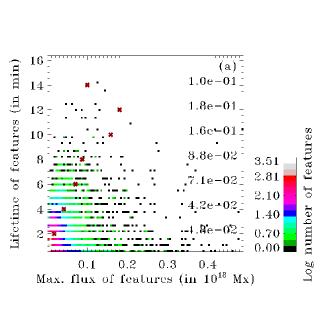
In Fig. 12 (a) we present a 2D histogram of the number of features in the plane spanned by the feature lifetime and the maximum magnetic flux achieved by a feature during it’s lifetime. The plot is for area-ratio restricted to a maximum of 5:1. Clearly, the features with a very short lifetime (just 1 or at most a few frames) cover the full range of fluxes of features considered here, whereas the long-lived features have small flux. Interestingly, the region “high flux long-lived features” is very sparsely populated. For a better visibility of this, the range of plotted maximum flux of feature is limited to $5\times 10^{17}$ Mx. Although we do not plot a few features that have larger flux, their number is negligible compared with all the features (36 compared with a total of 15691 features). The over-plotted red diamond symbols represent the average value of the maximum flux of feature at each lifetime. This average includes also the features that lie outside the frame. It is now clearly visible from these diamond symbols that the maximum flux per feature on average although increases with lifetime for features living less than 12 minutes, it decreases with increasing lifetime for features living longer than 12 minutes. Since the area and the flux are linearly related, this means that big long-lived features are also rare. This is somewhat in contrast to the general expectation that larger magnetic features live longer, as is the case for sunspots at the extreme end of the area range. These follow the Gnevyshev-Waldmeier rule of Gnevyshev (1938) and Waldmeier (1955) (see also Solanki, 2003), that gives a linear relationship between area and lifetime. Of course, even the largest features we see here are smaller than sunspots or pores. The absence of “old big features” is mainly due to the fact that they tend to split and merge with other features rather quickly.

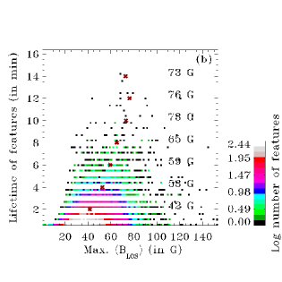
The relationship between lifetimes and LOS magnetic field is plotted in Fig. 12 (b). Here the largest LOS magnetic field component, spatially averaged over the magnetic feature, reached during the lifetime of the feature is displayed. The figure shows that short-lived features mostly appear in the magnetic field range of $0$ to $150$ G. There is a weak tendency for the LOS magnetic field to increase with lifetime (as can be gleaned from the bin-averaged values given in Fig. 12 (b), that are represented using red diamond symbols).

Figure 11: Histograms of lifetimes of the magnetic features for the area-ratio criterion 10:1 (panel a) and 2:1 (panel b). The red and the blue lines represent the power-law and the exponential fits respectively. The gray shaded histograms represent the lifetimes with a correction factor (see Section 4.5) and the yellow shaded histograms represent the lifetimes without any correction.

Figure 12: Lifetimes of features for an area ratio criterion 5:1 vs. maximum fluxes (panel a) and maximum, average magnetic field strength values from COG technique (panel b). Here maximum refers to the maximum value of the magnetic flux or the field strength, gained during the entire lifetime of the feature. In panel (a) the range of plotted maximum flux of feature is limited to $5\times 10^{17}$ Mx to enhance the visibility of flux-lifetime relationship. The over-plotted red diamond symbols represent the average value of the maximum flux of features at each lifetime (see main text for details). The maximum $\langle B_{\rm{LOS}}\rangle$ averaged over each lifetime bin are displayed in the figure and are represented by over-plotted red diamond symbols.

4.6 Evolution of magnetic features

We now consider the evolution of the magnetic fluxes of the features which live for at least 4 time steps (2 minutes). In Figs. 13–15 we plot feature-averaged fluxes as a function of normalized lifetimes. Fig. 13 shows growth and decay of all features that are born and died during the analyzed time series. On average, the fluxes in the features increase by $20-30$ % after their birth, reach a maximum after around $2/3$ of their lifetime lies behind them and then decrease again by $10-20$ % until their death. Consequently, the variation over the lifetime is relatively small. Interestingly, the features have on average a higher magnetic flux at the end of their lifetime than at the beginning. The dotted and solid curves are for the 2:1 and 10:1 area-ratio criterion, respectively. Only the evolution of magnetic flux is plotted since the area displays a nearly identical evolution.

The flux evolution of features depends sensitively on the method of birth and/or death, as is illustrated in Figs. 14 and 15. In Figs. 14 (a) and 14 (b) the magnetic flux evolution of features that undergo death by disappearance and cancellation is depicted, respectively. The magnetic flux of such features peaks nearly in the middle of their lifetime, and drops rapidly after that, reaching a value that is on average half of their peak flux. Note that, although the features considered here have died by disappearance and cancellation, these features could be born by any type of birth event. Therefore the curves depend on the area-ratio criterion. In Figs. 14 (c) and 14 (d) we display the evolution of features that die only due to splitting and merging respectively. These display nearly the opposite evolution, with the flux growing (by a factor of roughly $1.3-1.8$) until nearly the time of death.

In Figs. 15 (a) and 15 (b) the evolution of features that are born by appearance and emergence are plotted respectively, while Figs. 15 (c) and 15 (d) show the evolution of features that are born exclusively by splitting and merging, respectively.

The growth and decay of magnetic flux over a feature’s lifetime often behaves differently for the two extreme area-ratio criteria. In most cases with sufficiently large samples of features the two curves display a qualitatively similar shape, but have different magnitudes, corresponding to different amounts of magnetic flux per considered feature. The flux per feature is larger for the 10:1 area ratio criterion in the cases of the features dying by splitting and merging. This is because, in the liberal 10:1 case, a big feature dies even if only a small part of it breaks off, whereas in the 2:1 case such a big feature would continue to live on. Hence, a feature that is counted only once in the 2:1 is counted multiple times in the 10:1 case, so that the average flux per feature is increased.

Conversely, for the features that died by disappearance and cancellation, the average flux per feature is larger for the 2:1 area-ratio criterion. This is because, in the 10:1 case, most big features die by splitting and merging and the remaining smaller features, those which die by disappearance or cancellation, begin their journey with a smaller flux and have relatively shorter life times. In the 2:1 case, far fewer big features die by splitting and merging and therefore they have higher initial flux and longer life times (see also Fig. 11). Since here we consider only features which live at least for 4 time frames, the above argument leads to a larger flux per feature for the 2:1 case. However note that the initial flux of the features in Fig. 14 is the average of the initial fluxes of the features that are born by any birth event. Therefore the initial fluxes behave differently, in comparison to the behavior of the average flux per feature discussed above.

The features that die by cancellation and disappearance show smaller fluxes than the features that die by splitting and merging. At their death, the flux of disappearing and cancelling features is smaller than the flux at their births, which is not surprising, since these processes either remove flux from the solar surface, or redistribute it in such a way that it gets hidden from observations of Stokes $V$. Possible ways of flux removal are by retraction of a small magnetic loop, often preceded by magnetic reconnection, or the ejection of a $U$-loop (e.g. produced by reconnection below the solar surface), or an $O$-loop, or the dissipation of magnetic flux structured at very small scales. Flux at the solar surface can be hidden by, e.g., diffusion of the flux until the Stokes $V$ signal it produces drops below the noise level, or by the splitting of small magnetic features, so that the resulting features are below the flux limit, by bringing opposite polarity features close to each other (opposite polarities within a resolution element lead to the cancellation of Stokes $V$ signals), or increased inclination of the magnetic field. The last of these processes works even when considering the full Stokes vector because for a given noise level in Stokes $Q$, $U$, $V$, it requires nearly an order of magnitude larger horizontal magnetic flux (in the line formation layer) per pixel for a $Q$ or $U$ signal to be visible above the noise than vertical magnetic flux for it to be detectable in Stokes $V$ (see also Lamb et al., 2013, and the references cited therein).

Features that die due to splitting and merging reach their largest fluxes in the second half of their lifetimes. On average, they have higher fluxes at the time of their death than at birth. Clearly, it is the biggest features that tend to split. This is very similar to the behavior of granules, where it is also the larger granules that are likely to split (see Hirzberger et al., 1999), although the physical reasons are likely to be different. We note that at least partly the tendency for the big features to split is a result of a bias: if a feature with an area of less than 10 pixels splits, at least one of the children will be below the minimum size requirement of 5 pixels, so that no splitting will be seen. Indeed, if the area is 8 pixels or less, the feature might even “disappear” according to our criteria.

In Figs. 15 (a)–15 (d) the evolution of features classified according to their birth type are shown, which can be explained using similar arguments used for understanding the evolution of the features classified according to death, discussed above.

Figure 13: Average growth and decay of fluxes of all the features with area-ratio criterion 10:1 (solid line, averaged over $3632$ features) and 2:1 (dotted line, averaged over $3459$ features). These features live for at least 4 time steps (2 minutes).

Figure 14: (a) Same as Fig. 13, but for the features that die by disappearance for area-ratio criterion 10:1 (solid line, averaged over $1994$ features) and 2:1 (dotted line, averaged over $2224$ features). (b) Same as (a) for features that die by cancellation (averaged over $113$ and $126$ features for 10:1 and 2:1 respectively). (c) Same as (a) for features that die by splitting (averaged over $804$ and $523$ features for 10:1 and 2:1 respectively). (d) Same as (a) for features that die by merging (averaged over $687$ and $333$ features for 10:1 and 2:1 respectively).

Figure 15: (a) Same as Fig. 13, but for features born by appearance for area-ratio criterion 10:1 (solid line, averaged over $2116$ features) and 2:1 (dotted line, averaged over $2425$ features). (b) Same as (a) for features born by emergence (averaged over $64$ and $25$ features for 10:1 and 2:1 respectively). (c) Same as (a) for features born by splitting (averaged over $791$ and $375$ features for 10:1 and 2:1 respectively). (d) Same as (a) for features born by merging (averaged over $631$ and $413$ features for 10:1 and 2:1 respectively).

5 Conclusions

In this paper we present a newly developed feature tracking algorithm and use it to study the evolution of small-scale magnetic features present in quiet-Sun high spatial and temporal resolution observations made by the IMaX instrument on the Sunrise balloon-borne observatory. We use the COG technique of Rees & Semel (1979) for deducing the LOS components of the magnetic field, from which we determine the magnetic flux. We apply the technique to Stokes $V$ signals spatially averaged over the magnetic features. The feature-averaged magnetic field strength values thus obtained range between $50-150$ G. Note, however, that maximum field strengths can reach kG values as shown in Fig. 2 even when assuming that the features are spatially resolved (see also Lagg et al., 2010; Requerey et al., 2014; Riethmüller et al., 2014).

We focus our attention on the processes by which these features are born or die, namely birth by uni-polar appearance, splitting, merging, bi-polar emergence, death by uni-polar disappearance, splitting, merging and by cancellation of opposite polarities.

Qualitatively our result agrees with other recent studies (see e.g., Lamb et al., 2008, 2013). In summary, bi-polar emergence events are rare compared to the birth of the magnetic features by uni-polar events, emergence being responsible for only $0.3-0.5$ % of the total instantaneous flux and only $0.5-1$ % of the total maximum flux in newborn features. On the other hand, appearances account for $12$ % of the total instantaneous flux and $19.1$ % of the total maximum flux, which are much higher than the fluxes in emergence events. The remaining flux is distributed in splitting, merging and merging-into birth events. When only appearance and emergence are considered as birth events (leaving out splitting and merging), flux gained in appearance accounts for $92.4$ % of the total instantaneous flux, and $91$ % of the total maximum flux of the new flux at the solar surface. The remaining flux is is divided among the features involved in time-symmetric and time-asymmetric emergences.

Death by cancellation corresponds to $1.7$ % of the total instantaneous flux and $2.9$ % of the total maximum flux for the area ratio criterion of 10:1, while disappearance corresponds to a higher flux loss, which is $10.3$ % of the total instantaneous flux and $16.2$ % of the total maximum flux. The remaining flux is distributed in other uni-polar death types, namely, splitting, merging and splitting-off events. When only disappearance and cancellation are considered as death events (leaving out splitting and merging), cancellation leads to $14$ % of the total instantaneous flux and $15$ % of the total maximum flux. The features that survive in semi and partial cancellation also remove flux. After including this, the flux lost in disappearance is $59$ %, flux lost in cancellation leading to death of features and in those surviving cancellation is respectively, $10$ % and $31$ %.

The fact that a large number of features simply appear and disappear, without any clear sign of an opposite polarity, is partly due to the limited spatial resolution of the Sunrise/IMaX observations (although higher than that of the data used for previous such studies). E.g., if two features with sizes below the threshold of $5$ pixels each merge, then the resulting feature can be larger than this threshold. It will then be seen to have simply appeared. Similarly, a feature of $5-8$ pixels can either split into two features that are below the resolution threshold of $5$ pixels so that it disappears, or equivalently, it can partially cancel with a feature just below the $5$ pixel threshold and also disappear. Such interactions, as well as those with features hidden because their Stokes $V$ signals are not sufficiently above the noise, will go undetected.

The lifetime of the magnetic features follows a distribution whose exact shape is not completely clear. Thus it is best described by a power law for the 2:1 area-ratio criterion and an exponential function for the 10:1 area-ratio criterion. These functions agree with those suggested by Lamb et al. (2013, Hinode data) for the 2:1 area-ratio while for the 10:1 case the best-fit function agrees with Zhou et al. (2010, Hinode data). The power-law fit index ranges from $-3.2$ to $-3.7$ and the exponential fit index ranges between $-0.5$ to $-0.7$.

The area, instantaneous flux and maximum flux of the magnetic features also follow power-law-type distributions with exponents of $-2.25$, $-1.85$ and $-1.78$, respectively. They are in agreement with previous studies, by Buehler et al. (2013, area distribution, Hinode data) and Parnell et al. (2009, flux distribution, several data sets of last two decades), Iida et al. (2012, flux distribution, Hinode data). However we find that the power-law indices sensitively depend on the smallest flux per feature chosen and, even more strongly, on the type of binning. Because of the higher spatial resolution of Sunrise/IMaX instrument we can detect features of flux as low as $9\times 10^{14}$ Mx which is nearly an order of magnitude lower than the lowest flux detected in previous studies using Hinode data.

We also studied the growth and decay of the features. This study suggests that the features that appear, disappear, emerge and cancel carry low amounts of magnetic flux when compared to the fluxes in the features that split and merge. This suggests that the largest features are those who tend to split, followed by those who merge, and finally those who disappear and cancel.

Table 1: Parameters of fits to flux distributions in Figs. 8 and 9.

	Fit parameters for Fig 8
Type	Instantaneous flux	Maximum flux
Minimum value of flux	$8.8\times 10^{14}$ Mx	$9\times 10^{14}$ Mx
Power law index	-1.85	-1.78
$\chi^{2}$ of the fit	63.7	28.3
	Fit parameters for Fig 9
Type	Instantaneous flux	Maximum flux
Minimum value of flux	$4.7\times 10^{15}$ Mx	$4.8\times 10^{15}$ Mx
Power law index	-0.97 (Blue)	-1.04 (Blue)
$\chi^{2}$ of the fit	2.03	2.16
Minimum value of flux	$2\times 10^{16}$ Mx	$2\times 10^{16}$ Mx
Power law index	-1.16 (Red)	-1.23 (Red)
$\chi^{2}$ of the fit	0.69	0.93
Minimum value of flux	$8\times 10^{16}$ Mx	$8\times 10^{16}$ Mx
Power law index	-1.19 (Purple)	-1.33 (Purple)
$\chi^{2}$ of the fit	0.65	0.77
Minimum value of flux	$2\times 10^{17}$ Mx	$2\times 10^{17}$ Mx
Power law index	-1.03 (Green)	-1.26 (Green)
$\chi^{2}$ of the fit	0.52	0.74

Table 2: Number of features born as well as the number that died due to different processes, as listed in the first column of the table. The following columns give the number of features involved in birth and death events of a certain type, as well as their percentage contribution to all features that are born, or have died, respectively. The individual columns differ in the applied area-ratios of splitting and merging features or flux ratios of emerging features (see text for details).

	Area-ratio criteria
Type of birth	10:1	5:1	3:1	2:1
Appearance	8728	8834	8922	8984
	(48 %)	(52 %)	(55 %)	(59 %)
Splitting	6072	4879	3757	2505
	(34 %)	(28 %)	(23 %)	(17 %)
Merging	2226	1846	1432	965
	(12 %)	(11 %)	(9 %)	(6 %)
Splitting-off	646	1287	1887	2561
	(4 %)	(7.5 %)	(12 %)	(17 %)
Emerging	365	259	171	109
	(2 %)	(1.5 %)	(1 %)	(1 %)
Alive in first frame	1019	1019	1019	1019
Total	19056	18124	17188	16143
Type of death	10:1	5:1	3:1	2:1
Disappearance	7533	7533	7533	7533
	(42.7 %)	(44.8 %)	(47.3 %)	(50.6 %)
Splitting	2843	2277	1753	1177
	(16 %)	(14 %)	(11 %)	(8 %)
Merging	5226	4232	3206	2120
	(29 %)	(25 %)	(20 %)	(14 %)
Merging-into	627	1255	1869	2486
	(4 %)	(7 %)	(12 %)	(17 %)
Cancelling	1550	1550	1550	1550
	(8.7 %)	(9.2 %)	(9.7 %)	(10.4 %)
Alive in last frame	1277	1277	1277	1277
Total	19056	18124	17188	16143

Table 3: Same as Table 2, but listing the total magnetic flux (in Mx) of the features at the time of their birth or death (first line of each row). Fractional contribution of a certain type of birth/death to the total amount of flux in newly born or dying features is expressed in % and is given in the second line of each row. The average flux per feature is given in the third line of each row.

	Area-ratio criteria
Type of birth	10:1	5:1	3:1	2:1
Appearance: total	4.7$\times 10^{19}$ Mx	4.8$\times 10^{19}$ Mx	4.8$\times 10^{19}$ Mx	4.8$\times 10^{19}$ Mx
(%)	(12 %)	(16.5 %)	(21 %)	(27 %)
Average flux per feature	5.4$\times 10^{15}$ Mx	5.4$\times 10^{15}$ Mx	5.4$\times 10^{15}$ Mx	5.4$\times 10^{15}$ Mx
Splitting: total	1.8$\times 10^{20}$ Mx	1.2$\times 10^{20}$ Mx	8.2$\times 10^{19}$ Mx	5.3$\times 10^{19}$ Mx
(%)	(44.5 %)	(41 %)	(36 %)	(29.3 %)
Average flux per feature	2.9$\times 10^{16}$ Mx	2.5$\times 10^{16}$ Mx	2.2$\times 10^{16}$ Mx	2.1$\times 10^{16}$ Mx
Merging: total	1.6$\times 10^{20}$ Mx	1.1$\times 10^{20}$ Mx	7.9$\times 10^{19}$ Mx	5.2$\times 10^{19}$ Mx
(%)	(41.5 %)	(38 %)	(34.6 %)	(28.8 %)
Average flux per feature	7.4$\times 10^{16}$ Mx	6.0$\times 10^{16}$ Mx	5.5$\times 10^{16}$ Mx	5.4$\times 10^{16}$ Mx
Splitting-off: total	5.8$\times 10^{18}$ Mx	1.1$\times 10^{19}$ Mx	1.9$\times 10^{19}$ Mx	2.6$\times 10^{19}$ Mx
(%)	(1.5 %)	(4 %)	(8 %)	(14.6 %)
Average flux per feature	8.9$\times 10^{15}$ Mx	8.9$\times 10^{15}$ Mx	9.9$\times 10^{15}$ Mx	1.0$\times 10^{16}$ Mx
Emerging: total	1.9$\times 10^{18}$ Mx	1.4$\times 10^{18}$ Mx	9.4$\times 10^{17}$ Mx	5.7$\times 10^{17}$ Mx
(%)	(0.5 %)	(0.5 %)	(0.4 %)	(0.3 %)
Average flux per feature	5.4$\times 10^{15}$ Mx	5.7$\times 10^{15}$ Mx	5.9$\times 10^{15}$ Mx	5.8$\times 10^{15}$ Mx
Total	4.0$\times 10^{20}$ Mx	2.9$\times 10^{20}$ Mx	2.3$\times 10^{20}$ Mx	1.8$\times 10^{20}$ Mx
(%)	(100 %)	(100 %)	(100 %)	(100 %)
Type of death	10:1	5:1	3:1	2:1
Disappearance: total	4.3$\times 10^{19}$ Mx	4.3$\times 10^{19}$ Mx	4.3$\times 10^{19}$ Mx	4.3$\times 10^{19}$ Mx
(%)	(10.3 %)	(13.7 %)	(17.3 %)	(21.4 %)
Average flux per feature	5.8$\times 10^{15}$ Mx	5.8$\times 10^{15}$ Mx	5.8$\times 10^{15}$ Mx	5.8$\times 10^{15}$ Mx
Splitting: total	1.9$\times 10^{20}$ Mx	1.3$\times 10^{20}$ Mx	8.8$\times 10^{19}$ Mx	5.7$\times 10^{19}$ Mx
(%)	(45.2 %)	(41.6 %)	(35 %)	(28 %)
Average flux per feature	6.7$\times 10^{16}$ Mx	5.8$\times 10^{16}$ Mx	5.0$\times 10^{16}$ Mx	4.8$\times 10^{16}$ Mx
Merging: total	1.6$\times 10^{20}$ Mx	1$\times 10^{20}$ Mx	7.3$\times 10^{19}$ Mx	4.8$\times 10^{19}$ Mx
(%)	(38.4 %)	(33.4 %)	(29.1 %)	(23.6 %)
Average flux per feature	3.1$\times 10^{16}$ Mx	2.5$\times 10^{16}$ Mx	2.3$\times 10^{16}$ Mx	2.3$\times 10^{16}$ Mx
Merging-into: total	1.8$\times 10^{19}$ Mx	2.8$\times 10^{19}$ Mx	3.9$\times 10^{19}$ Mx	4.8$\times 10^{19}$ Mx
(%)	(4.4 %)	(9 %)	(15.7 %)	(23.4 %)
Average flux per feature	2.9$\times 10^{16}$ Mx	2.3$\times 10^{16}$ Mx	2.1$\times 10^{16}$ Mx	1.9$\times 10^{16}$ Mx
Cancelling: total	7.3$\times 10^{18}$ Mx	7.3$\times 10^{18}$ Mx	7.3$\times 10^{18}$ Mx	7.3$\times 10^{18}$ Mx
(%)	(1.7 %)	(2.3 %)	(2.9 %)	(3.6 %)
Average flux per feature	4.7$\times 10^{15}$ Mx	4.7$\times 10^{15}$ Mx	4.7$\times 10^{15}$ Mx	4.7$\times 10^{15}$ Mx
Total	4.2$\times 10^{20}$ Mx	3.1$\times 10^{20}$ Mx	2.5$\times 10^{20}$ Mx	2.$\times 10^{20}$ Mx
(%)	(100 %)	(100 %)	(100 %)	(100 %)

Table 4: Normalized, maximum flux distribution of the features involved in the various types of birth and death processes.

	Area-ratio criteria
Type of birth	10:1	5:1	3:1	2:1
Appearance	19.1 %	25.1 %	32 %	39.5 %
Splitting	41.8 %	36 %	29.2 %	22 %
Merging	36.5 %	33 %	29.1 %	23 %
Splitting-off	1.6 %	5.0 %	9.0 %	15 %
Emerging	1.0 %	0.9 %	0.7 %	0.5 %
Total	100 %	100 %	100 %	100 %
Type of death	10:1	5:1	3:1	2:1
Disappearance	16.2 %	20.8 %	25.3 %	30.9 %
Splitting	42.3 %	38.4 %	32.2 %	25 %
Merging	34.7 %	29.4 %	24.6 %	19.5 %
Merging-into	3.9 %	7.8 %	13.3 %	19 %
Cancelling	2.9 %	3.6 %	4.6 %	5.6  %
Total	100 %	100 %	100 %	100 %

Table 5: Flux distribution in different types of emergence and cancellation events (see Sect. 4.3.2).

	Emergence events
Area-ratio	10:1	5:1	3:1	2:1
Fractional instantaneous flux
Time-symmetric emergence	3 %	4 %	6 %	10 %
Time-asymmetric emergence	97 %	96 %	94 %	90  %
Fractional maximum flux
Time-symmetric emergence	4 %	5 %	9 %	14 %
Time-asymmetric emergence	96 %	95 %	91 %	86  %
	Cancellation events
Area-ratio	10:1	5:1	3:1	2:1
Fractional instantaneous flux
Complete cancellation	2 %	2 %	2 %	2 %
Semi and partial cancellation	98 %	98 %	98 %	98 %
Fractional maximum flux
Complete cancellation	3 %	2 %	2 %	2 %
Semi and partial cancellation	97 %	98 %	98 %	98 %

Table 6: Comparison of our results with previous studies (see Sect. 4.4 for details).

Birth events	Previous studies	Present study	Present study
		(fractional instantaneous flux)	(fractional maximum flux)
Appearance	12 % (Lamb et al., 2008)	12 %	19.1 %
Fragmentation	76 % (Lamb et al., 2008)	44.5 % splitting	41.8 % splitting
(Splitting/Merging)		41.5 % merging	36.5 % merging
Emergence	1 % (Lamb et al., 2008)	1 %	2 %
Death events	Previous studies	Present study	Present study
		(instantaneous flux)	(maximum flux)
Disappearance	83 % (Lamb et al., 2013)	86 %	85 %
Cancellation	12 % (Lamb et al., 2013)	14 %	15 %

Table 7: Parameters of fits to lifetime distributions.

	Area-ratio criteria
	10:1	5:1	3:1	2:1
Power law index	-3.7	-3.7	-3.3	-3.2
$\chi^{2}$ of the fit	7.1	5.9	3.5	3.5
Exponential-fit index	-0.7	-0.6	-0.5	-0.5
$\chi^{2}$ of the fit	3.6	4.9	3.8	4.4

Appendix A Quantitative definitions of splitting and merging events

Below we provide precise quantitative definitions of splitting and merging events.

Let $N_{a}$ denote the number of features at time $t_{2}$ that spatially overlap with a feature labeled as $a$ at $t_{1}$. Let $N_{b}$ denote the number of features at $t_{1}$ that spatially overlap with a feature labeled as $b$ at $t_{2}$. Let $b_{i},i=1,2,...,N_{a}$ denote the features that spatially overlap with $a$, and $a_{i},i=1,2,...,N_{b}$ denote the features that spatially overlap with $b$. Let both $b_{i}$ and $a_{i}$ be ordered, in decreasing order of their areas. Let $n_{s}:1$ denote the general area-ratio criterion, with $n_{s}=2,3,5$.

$\bullet$ Criteria for an event to be classified as a splitting event, a disappearance, or not to be considered as a death/birth event at all :

$N_{a}>1$ : If $n_{s}\times$ area($b_{2}$) ¿ area($b_{1}$) then $a$ splits into $b_{i},i=1,2,...,N_{a}$. If $n_{s}\times$ area($b_{2}$) ¡ area($b_{1}$) then $a$ continues to live as $b_{1}$ and the remaining features $b_{i},i=2,...,N_{a}$ are considered to be newly born at $t_{2}$ by splitting off from $a$.

$N_{a}=1$ : In this case, $a$ spatially overlaps with only one feature $b_{1}$ and therefore $a$ continues to live as $b_{1}$ at $t_{2}$.

$N_{a}=0$ : Here, $a$ does not spatially overlap with any of the features at $t_{2}$ and hence it simply dies at $t_{1}$.

$\bullet$ Criteria for an event to be classified as a merging event, an appearance, or not to be considered as a death/birth event:

$N_{b}>1$ : If $n_{s}\times$ area($a_{2}$) ¿ area($a_{1}$) then $a_{i},i=1,2,...,N_{b}$ merge together to form the feature $b$. If $n_{s}\times$ area($a_{2}$) ¡ area($a_{1}$) then $a_{1}$ continues to live as $b$ and the remaining features $a_{i},i=2,...,N_{b}$ are considered to be dead at $t_{1}$ by merging into $b$.

$N_{b}=1$ : Here, $b$ spatially overlaps with only one feature $a_{1}$ and therefore $a_{1}$ at $t_{1}$ continues to live as $b$ at $t_{2}$.

$N_{b}=0$ : Here, $b$ does not spatially overlap with any of the features at $t_{1}$ and hence it is simply born at $t_{2}$.

Appendix B Simultaneous events and ambiguities

From one time step to the next, say, $t_{1}$ to $t_{2}$, either a feature may continue to live or it may die, not continuing to live on to $t_{2}$, i.e. the feature dies at $t_{1}$. Clearly, a feature cannot live on and die at the same time. However, in some cases described below, when multiple events happen simultaneously, ambiguities regarding life and death of a given feature can arise. To resolve such ambiguities, first we define priorities for different events.

(1) Primary, i.e. highest priority, events : Death of parent features due to splitting or death of parent features due to merging.

(2) Secondary events : Feature with largest area continues to live through splitting or merging event, because area-ratio is not met.

(3) Tertiary, i.e. lowest priority, events : Death of features with smaller area when feature with largest area lives on. This happens when the area-ratio criterion is not met for merging features.

A given feature $a$ at a given time $t_{1}$ can undergo one of the following events independently.

(i) $E_{1}$ : Split into child features, say into $b_{1}$ and $b_{2}$, while satisfying an imposed area-ratio condition.

(ii) $E_{2}$ : Merge with another parent feature $a_{1}$ while satisfying an imposed area-ratio condition, to form a new feature $b$.

(iii) $E_{3}$ : Split into multiple features, say $b_{3}$ and $b_{4}$, but not satisfying the imposed area-ratio condition. So in effect the feature $a$ lives on as the feature with largest area among its children, i.e. among $b_{3}$ and $b_{4}$.

(iv) $E_{4}$ : Merge with another feature, say $a_{2}$ not satisfying the imposed area-ratio condition, to form a child feature, say $b_{5}$. Then the feature with largest area among $a$ and $a_{2}$ lives on as $b_{5}$.

In Fig. 16 a cartoon diagram describes these events visually, with the condition area$(b_{4})$ ¿ area$(b_{3})$ in $E_{3}$ and area$(a)$ ¿ area$(a_{2})$ in $E_{4}$.

Among the above four events, we can form six non-empty sets as $E_{i}\cap E_{j}$, $i,j=1,2,3,4$, $i\neq j$ (note here that for any $i\neq j$, $E_{i}\cap E_{j}=E_{j}\cap E_{i}$). Although $E_{1}$ and $E_{3}$ can happen simultaneously, they can be treated as a single splitting event with multiple child features, which can be handled unambiguously. Similarly, $E_{2}$ and $E_{4}$ happening simultaneously can be handled as a single merging event, without any ambiguity. Therefore we do not discuss these straightforward cases here. We describe each of the other 4 possibilities in the following and the respective solutions for the ambiguities. In Fig. 16 we show these events in a cartoon diagram. Always left panels represent $t=t_{1}$ and the right panels $t=t_{2}$.

1. $E_{1}\cap E_{2}\neq\emptyset$ : In this case, in the same time step $a$ splits into two ($E_{1}$) and merges with another magnetic feature ($E_{2}$). Event $E_{1}$ leads to the death of the feature $a$, and event $E_{2}$ leads to the death of features $a$ and $a_{1}$, and together these 2 events lead to the birth of features $b_{1}$, $b_{2}$ and $b$ at $t_{2}$. Note that either of $b_{1}$, $b_{2}$ could be the same feature as $b$. Consequently, this simultaneous event does not lead to any ambiguity.

2. $E_{1}\cap E_{4}\neq\emptyset$ : In this case, $E_{1}$ leads to the death of $a$ and $E_{4}$ leads to a continued life of $a$ or $a_{2}$ as $b_{5}$. Here we have two sub cases as follows.

(i) area$(a)$ ¿ area$(a_{2})$ : In this case, $E_{4}$ leads to a continued life of $a$, which will live as $b_{5}$ at $t_{2}$. This leads to an ambiguity of life and death of $a$. Since $E_{1}$ is a primary event, it is given the higher priority over the secondary event $E_{4}$. Thus, $a$ dies as a result of $E_{1}$ and $a_{2}$ also dies because it is the smaller counter part in the merging event.

(ii) area$(a_{2})$ ¿ area$(a)$ : In this case, $E_{4}$ leads to a continued life of $a_{2}$ which will live as $b_{5}$ at $t_{2}$. There is no ambiguity in this case.

3. $E_{2}\cap E_{3}\neq\emptyset$ : In this case, $E_{2}$ leads to the death of $a$ and $a_{1}$ and $E_{3}$ leads to a continued life of $a$ which would live on as $b_{3}$ or $b_{4}$. Therefore there is an ambiguity of whether $a$ lives or dies. Since $E_{2}$ is given a higher priority over $E_{3}$, $a$ and $a_{1}$ die as a result of $E_{2}$, and $b_{3}$ and $b_{4}$ are considered to be newly born at $t_{2}$.

4. $E_{3}\cap E_{4}\neq\emptyset$ : In this case, $E_{3}$ leads to a continued life of $a$ which will live as $b_{3}$ or $b_{4}$ and $E_{4}$ leads to a continued life of $a$ or $a_{2}$ as $b_{5}$. Note that for this simultaneous event to occur, we have named the features at $t_{2}$ such that area$(b_{5})$ is smaller than area$(b_{3})$ and area$(b_{4})$. Here we have four sub cases similar to cases 3 and 5 above. This is a complex situation because both $E_{3}$ and $E_{4}$ are not primary events. Therefore let us consider the four sub-cases in detail.

(i) area$(b_{3})$ ¿ area$(b_{4})$ and area$(a)$ ¿ area$(a_{2})$ : Here $E_{3}$ leads to a continued life of $a$ as $b_{3}$ at $t_{2}$. $E_{4}$ leads to a continued life of $a$ as $b_{5}$. The smaller counterpart of the merging event $a_{2}$ will simply die. This case leads to an ambiguity between whether $a$ continues to live as $b_{3}$ or as $b_{5}$. Since $a$ spatially overlaps with $b_{3}$, $b_{4}$ and $b_{5}$, actually $b_{5}$ can also be considered to be a child of the splitting of $a$. Since we have named the features at $t_{2}$ such that area$(b_{5})$ ¡ area$(b_{3})$ and area$(b_{5})$ ¡ area$(b_{4})$, we let $a$ live as the feature with largest area at $t_{2}$, namely, $b_{3}$. The features $b_{4}$ and $b_{5}$ are considered to be newly born.

(ii) area$(b_{4})$ ¿ area$(b_{3})$ and area$(a)$ ¿ area$(a_{2})$ : This case is the same as case (i) above with the roles of $b_{3}$ and $b_{4}$ interchanged. Here $a$ lives on as $b_{4}$.

(iii) area$(b_{3})$ ¿ area$(b_{4})$ and area$(a_{2})$ ¿ area$(a)$ : Here $E_{3}$ leads to a continued life of $a$ as $b_{3}$ at $t_{2}$. $E_{4}$ leads to a continued life of $a_{2}$ as $b_{5}$. The smaller counterpart of the merging event that dies in this case is $a$. This leads to an ambiguity between the life and death of $a$.

Since $E_{3}$ leads to the life of a bigger counterpart of the splitting event and $E_{4}$ leads to the death of smaller counter part of the merging event. Since $E_{3}$ is a secondary event, while $E_{4}$ is a tertiary event, $E_{3}$ is given the higher priority over $E_{4}$ and hence $a$ continues to live as $b_{3}$.

(iv) area$(b_{4})$ ¿ area$(b_{3})$ and area$(a_{2})$ ¿ area$(a)$ : Here $a_{2}$ continues to live as $b_{5}$ at $t_{2}$.

This case is the same as case (iii) above with the roles of $b_{3}$ and $b_{4}$ interchanged.

We remark here that two similar events can also happen simultaneously (e.g., two events of type $E_{3}$). The disambiguations employed for these cases are similar to those discussed above.

Figure 16: Events $E_{i}$, $i=1,2,3,4$ are shown with the conditions that area$(b_{4})$ ¿ area$(b_{3})$ in $E_{3}$ and area$(a)$ ¿ area$(a_{2})$ in $E_{4}$.

Appendix C Flow-diagrams for same polarity and opposite polarity interactions

Figure 17: Flowchart describing the code structure for unipolar interactions.

Figure 18: Flowchart describing the code structure for bi-polar interactions.

C.1 Description of algorithm

In this section we briefly give the computing algorithm for studies involving interactions between same-polarity features. The terms used here are defined in Section 3.3. A flowchart describing the corresponding computer code is given in Fig. 17.

Step 1: A lane-finding code is used to detect the features (see Hirzberger et al., 1999).

Step 2: The features at two successive time steps are checked for a spatial overlap. The number of features at time step $t_{2}$ which spatially overlaps with each of the features at $t_{1}$ are counted.

Step 3: If the parent feature $a_{1}$ at $t_{1}$ spatially overlaps with more than one child feature at $t_{2}$, then the areas of all these child features at $t_{2}$ are calculated. An area-ratio criterion is checked between the child features. We consider four cases, namely, 2:1, 3:1, 5:1 or 10:1.

Step 4: If the case-specific area-ratio criterion is satisfied between the two largest child features, then it is counted as a splitting event.

Step 5: If the area-ratio criterion is not satisfied, then the parent feature is considered to live on at time $t_{2}$ without splitting, in the form of the largest child feature. All the smaller child features are counted as newly born features at $t_{2}$, classified under splitting-off birth events.

Step 6: If the parent feature $a_{1}$ at $t_{1}$ spatially overlaps with only one child feature at $t_{2}$, then either it is considered to live on without any interaction at $t_{2}$, or it could be participating in a merging event. In the second case, the decision made at this stage will be overridden by the decisions taken at the stage where the merging events are studied in this sequence.

Step 7: If the parent feature $a_{1}$ at $t_{1}$ spatially overlaps with no child features at $t_{2}$, then it is considered to be dead without any interaction (disappearing feature).

Step 8: The number of features which stay up to the last time step of the observations are counted and are considered to live on (form of death remains undefined).

Step 9: At the same time step $t_{1}$, the number of features that spatially overlap with each of the features at $t_{2}$ are counted.

Step 10: If more than one parent features at $t_{1}$ spatially overlaps with a given feature $a_{2}$ at $t_{2}$, then the areas of all these parent features at $t_{1}$ are calculated. An area-ratio criterion is checked between the parent features. We consider four cases, namely, 2:1, 3:1, 5:1 or 10:1.

Step 11: If the case-specific area-ratio criterion is satisfied between the two largest parent features, then it is counted as a merging event.

Step 12: An additional check is made for the presence of simultaneous splitting and merging events (see Appendix B for more details).

Step 13: If the area-ratio criterion is not satisfied, then the largest parent feature is considered to live on at $t_{2}$ without merging. All the smaller parent features are counted as features that die at $t_{1}$ classified under merging-into death events.

Step 14: If the child feature $a_{2}$ at $t_{2}$ spatially overlaps with only one parent feature at $t_{1}$, and if that one parent feature, say, $a_{1}$ also spatially overlaps with only one feature $a_{2}$ at $t_{2}$, then $a_{1}$ is considered to live on without any interaction at $t_{2}$.

Step 15: If the child feature $a_{2}$ at $t_{2}$ spatially overlaps with no parent features at $t_{1}$, then it is a newly born feature and no special considerations are needed for this case (appearing features).

C.2 Description of algorithm : Mixed polarity interaction

In this section we briefly describe the computing algorithm for studies involving interactions between opposite polarity features. A flowchart describing the corresponding computer code is given in Fig. 18.

Step 1: A lane-finding code is used to detect features with both the polarities. The resulting data sets are stored as two cubes, one for positive and the other for negative features. These cubes are referred to as the original cubes.

Step 2: A two-step dilation is applied to the original cubes and the resulting data sets are stored as two dilated cubes.

Step 3: The dilated cubes are again used as input cubes in the lane finding code to detect the features which are connected after the dilation (meaning, spatially overlapping after dilation). The resulting data sets are again stored as two cubes. These are referred to as dilated-connected cubes.

Step 4: At time step $t_{1}$, first a spatial overlap of one or more positive features with one or more negative features are detected using the dilated-connected cubes (see step 3 above for definition). Then we apply a flux-ratio criterion between the sets of positive and negative features. We consider four cases, namely, 10:1, 5:1, 3:1 and 2:1. I.e. if the ratio of total flux contained in the interacting positive polarity features to that in the interacting negative polarity features satisfies the imposed flux ratio criterion, then it is detected to be an emergence event.

Step 5: Further, we check if the features participating in the emergence event are time-symmetric or time-asymmetric (see Section 3.3).

Step 6: If at any time step, a spatial overlap of two sets of opposite polarity features leads to disappearance of both the sets of opposite polarity features, then we say it is a complete cancellation event. If the spatial overlap of two sets of opposite polarity features is found to satisfy the condition for cancellation according to Equation (3), leading to disappearance of features of only one polarity, then the event is considered to be a semi cancellation event.

Step 7: If at time step, a spatial overlap of two sets of opposite polarity features is found to satisfy the condition for cancellation as described in Equation (3), leading to survival of both the polarity features, then the event is identified as a partial cancellation event.