Regularity Theory and High Order Numerical Methods for the (1D)-Fractional Laplacian

Abstract.

This paper presents regularity results and associated high-order numerical methods for one-dimensional Fractional-Laplacian boundary-value problems. On the basis of a factorization of solutions as a product of a certain edge-singular weight $\omega$ times a “regular” unknown, a characterization of the regularity of solutions is obtained in terms of the smoothness of the corresponding right-hand sides. In particular, for right-hand sides which are analytic in a Bernstein Ellipse, analyticity in the same Bernstein Ellipse is obtained for the “regular” unknown. Moreover, a sharp Sobolev regularity result is presented which completely characterizes the co-domain of the Fractional-Laplacian operator in terms of certain weighted Sobolev spaces introduced in (Babuška and Guo, SIAM J. Numer. Anal. 2002). The present theoretical treatment relies on a full eigendecomposition for a certain weighted integral operator in terms of the Gegenbauer polynomial basis. The proposed Gegenbauer-based Nyström numerical method for the Fractional-Laplacian Dirichlet problem, further, is significantly more accurate and efficient than other algorithms considered previously. The sharp error estimates presented in this paper indicate that the proposed algorithm is spectrally accurate, with convergence rates that only depend on the smoothness of the right-hand side. In particular, convergence is exponentially fast (resp. faster than any power of the mesh-size) for analytic (resp. infinitely smooth) right-hand sides. The properties of the algorithm are illustrated with a variety of numerical results.

1. Introduction

Over the last few years nonlocal models have increasingly impacted upon a number of important fields in science and technology. The evidence of anomalous diffusion processes, for example, has been found in several physical and social environments [26, 30], and corresponding transport models have been proposed in various areas such as electrodiffusion in nerve cells [28] and ground-water solute transport [7]. Non-local models have also been proposed in fields such as finance [13, 14] and image processing [19, 20]. One of the fundamental non-local operators is the Fractional Laplacian $(-\Delta)^{s}$ ($0<s<1$) which, from a probabilistic point of view corresponds to the infinitesimal generator of a stable Lévy process [38].

The present contribution addresses theoretical questions and puts forth numerical algorithms for the numerical solution of the Dirichlet problem

(1.1) $$\left\{\begin{array}[]{rl}(-\Delta)^{s}u=f&\mbox{ in }\Omega,\\ u=0&\mbox{ in }\Omega^{c}\\ \end{array}\right.$$

on a bounded one-dimensional domain $\Omega$ consisting of a union of a finite number of intervals (whose closures are assumed mutually disjoint). This approach to enforcement of (nonlocal) boundary conditions in a bounded domain $\Omega$ arises naturally in connection with the long jump random walk approach to the Fractional Laplacian [38]. In such random walk processes, jumps of arbitrarily long distances are allowed. Thus, the payoff of the process, which corresponds to the boundary datum of the Dirichlet problem, needs to be prescribed in $\Omega^{c}$.

Letting $s$ and $n$ denote a real number ($0<s<1$) and the spatial dimension ($n=1$ throughout this paper), and using the normalization constant [17]

$$C_{n}(s)=\frac{2^{2s}s\Gamma(s+\frac{n}{2})}{\pi^{n/2}\Gamma(1-s)},$$

the fractional-Laplacian operator $(-\Delta)^{s}$ is given by

(1.2) $$(-\Delta)^{s}u(x)=C_{n}(s)\mbox{ P.V.}\int_{\mathbb{R}^{n}}\frac{u(x)-u(y)}{|x-y|^{n+2s}}\,dy.$$

Remark 1.1.

A number of related operators have been considered in the mathematical literature. Here we mention the so called spectral fractional Laplacian ${\mathcal{L}}_{s}$, which is defined in terms of eigenfunctions and eigenvalues $(v_{n},\lambda_{n})$ of the standard Laplacian ($-\Delta$) operator with Dirichlet boundary conditions in $\partial\Omega$: ${\mathcal{L}}_{s}[v_{n}]=\lambda_{n}^{s}v_{n}$. The operator ${\mathcal{L}}_{s}$ is different from $(-\Delta)^{s}$—since, for example, ${\mathcal{L}}_{s}$ admits smooth eigenfunctions (at least for smooth domains) $\Omega$ while $(-\Delta)^{s}$ does not; see [35].

Remark 1.2.

A finite element approach for problems concerning the operator ${\mathcal{L}}_{s}$ (cf. Remark 1.1) was proposed in [31] on the basis of extension ideas first introduced in [12] for the operator $(-\Delta)^{s}$ in $\mathbb{R}^{n}$ which were subsequently developed in [9] for the bounded-domain operator ${\mathcal{L}}_{s}$. As far as we know, however, approaches based on extension theorems have not as yet been proposed for the Dirichlet problem (1.1).

Various numerical methods have been proposed recently for equations associated with the Fractional Laplacian $(-\Delta)^{s}$ in bounded domains. Restricting attention to one-dimensional problems, Huang and Oberman [24] presented a numerical algorithm that combines finite differences with a quadrature rule in an unbounded domain. Numerical evidence provided in that paper for smooth right-hand sides (cf. Figure 7(b) therein) indicates convergence to solutions of (1.1) with an order $\mathcal{O}(h^{s})$, in the infinity norm, as the meshsize $h$ tends to zero (albeith orders as high as $\mathcal{O}(h^{3-2s})$ are demonstrated in that contribution for singular right-hand sides $f$ that make the solution $u$ smooth). Since the order $s$ lies between zero and one, the $\mathcal{O}(h^{s})$ convergence provided by this algorithm can be quite slow, specially for small values of $s$. D’Elia and Gunzburger [16], in turn, proved convergence of order $h^{1/2}$ for a finite-element solution of an associated one-dimensional nonlocal operator that approximates the one-dimensional fractional Laplacian. These authors also suggested that an improved solution algorithm, with increased convergence order, might require explicit consideration of the solution’s boundary singularities. The contribution [3], finally, studies the regularity of solutions of the Dirichlet problem (1.1) and it introduces certain graded meshes for integration in one- and two-dimensional domains. The rigorous error bounds and numerical experiments provided in [3] demonstrate an accuracy of the order of $h^{1/2}|\log h|$ and $h|\log h|$ for all $s$, in certain weighted Sobolev norms, for solutions obtained by means of uniform and graded meshes, respectively.

Difficulties in the numerical treatment of the Dirichlet problem (1.1) stem mainly from the singular character of the solutions of this problem near boundaries. A recent regularity result in this regards was provided in [32]. In particular, this contribution establishes the global Hölder regularity of solutions of the general $n$-dimensional version of equation (1.1) ($n\geq 1$) and it provides a certain boundary regularity result: the quotient $u(x)/\omega^{s}(x)$ remains bounded as $x\to\partial\Omega$, where $\omega$ is a smooth function that behaves like $\mbox{dist}(x,\Omega^{c})$ near $\partial\Omega$. This result was then generalized in [21], where, using pseudo-differential calculus, a certain regularity result is established in terms of Hörmander $\mu$-spaces: in particular, for the regular Sobolev spaces $H^{r}(\Omega)$, it is shown that if $f\in H^{r}(\Omega)$ for some $r>0$ then the solution $u$ may be written as $w^{s}\phi+\chi$, where $\phi\in H^{r+s}(\Omega)$ and $\chi\in H^{r+2s}_{0}(\Omega)$. Interior regularity results for the Fractional Laplacian and related operators have also been the object of recent studies [4, 15].

The sharp regularity results put forth in the present contribution, in turn, are related to but different from those mentioned above. Indeed the present regularity theorems show that the fractional Laplacian in fact induces a bijection between certain weighted Sobolev spaces. Using an appropriate version of the Sobolev lemma put forth in Section 4, these results imply, in particular, that the regular factors in the decompositions of fractional Laplacian solutions admit $k$ continuous derivatives for a certain value of $k$ that depends on the regularity of the right-hand side. Additionally, this paper establishes the operator regularity in spaces of analytic functions: denoting by $A_{\rho}$ the space of analytic functions in the Bernstein Ellipse $\mathcal{E}_{\rho}$, the weighted operator $K_{s}(\phi)=(-\Delta)^{s}(\omega^{s}\phi)$ maps $A_{\rho}$ into itself bijectively. In other words, for a right-hand side which is analytic in a Bernstein Ellipse, the solution is characterized as the product of an analytic function in the same Bernstein Ellipse times an explicit singular weight.

The theoretical treatment presented in this paper is essentially self-contained. This approach recasts the problem as an integral equation in a bounded domain, and it proceeds by computing certain singular exponents $\alpha$ that make $(-\Delta)^{s}(\omega^{\alpha}\phi(x))$ analytic near the boundary for every polynomial $\phi$. As shown in Theorem 3.7 a infinite sequence of such values of $\alpha$ is given by $\alpha_{n}=s+n$ for all $n\geq 0$. Morever, Section 3.2 shows that the weighted operator $K_{s}$ maps polynomials of degree $n$ into polynomials of degree $n$—and it provides explicit closed-form expressions for the images of each polynomial $\phi$.

A certain hypersingular form we present for the operator $K_{s}$ leads to consideration of a weighted $L^{2}$ space wherein $K_{s}$ is self-adjoint. In view of the aforementioned polynomial-mapping properties of the operator $K_{s}$ it follows that this operator is diagonal in a basis of orthogonal polynomials with respect to a corresponding inner product. A related diagonal form was obtained in the recent independent contribution [18] by employing arguments based on Mellin transforms. The diagonal form [18] provides, in particular, a family of explicit solutions in the $n$ dimensional ball in ${\mathbb{R}}^{n}$, which are given by products of the singular term $(1-|z|^{2})^{s}$ and general Meijer G-Functions. The diagonalization approach proposed in this paper, which is restricted to the one-dimensional case, is elementary and is succinctly expressed: the eigenfunctions are precisely the Gegenbauer polynomials.

This paper is organized as follows: Section 2 casts the problem as an integral equation, and Section 3 analyzes the boundary singularity and produces a diagonal form for the single-interval problem. Relying on the Gegenbauer eigenfunctions and associated expansions found in Section 3, Section 4 presents the aforementioned Sobolev and analytic regularity results for the solution $u$, and it includes a weighted-space version of the Sobolev lemma. Similarly, utilizing Gegenbauer expansions in conjunction with Nyström discretizations and taking into account the analytic structure of the edge singularity, Section 5 presents a highly accurate and efficient numerical solver for Fractional-Laplacian equations posed on a union of finitely many one-dimensional intervals. The sharp error estimates presented in Section 5 indicate that the proposed algorithm is spectrally accurate, with convergence rates that only depend on the smoothness of the right-hand side. In particular, convergence is exponentially fast (resp. faster than any power of the mesh-size) for analytic (resp. infinitely smooth) right-hand sides. A variety of numerical results presented in Section 6 demonstrate the character of the proposed solver: the new algorithm is significantly more accurate and efficient than those resulting from previous approaches.

2. Hypersingular Bounded-Domain Formulation

In this section the one-dimensional operator

(2.1) $$(-\Delta)^{s}u(x)=C_{1}(s)\mbox{ P.V.}\int_{-\infty}^{\infty}\left(u(x)-u(x-y)\right)|y|^{-1-2s}dy$$

together with Dirichlet boundary conditions outside the bounded domain $\Omega$, is expressed as an integral over $\Omega$. The Dirichlet problem (1.1) is then identified with a hypersingular version of Symm’s integral equation; the precise statement is provided in Lemma 2.3 below. In accordance with Section 1, throughout this paper we assume the following definition holds.

Definition 2.1.

The domain $\Omega$ equals a finite union

(2.2) $$\Omega=\bigcup_{i=1}^{M}(a_{i},b_{i})$$

of open intervals $(a_{i},b_{i})$ with disjoint closures. We denote $\partial\Omega=\{a_{1},b_{1},\dots,a_{M},b_{M}\}$.

Definition 2.2.

$C^{2}_{0}(\Omega)$ will denote, for a given open set $\Omega\subset\mathbb{R}$, the space of all functions $u\in C^{2}(\Omega)\cap C(\mathbb{R})$ that vanish outside of $\Omega$. For $\Omega=(a,b)$ we will simply write $C^{2}_{0}((a,b))=C^{2}_{0}(a,b)$.

The following lemma provides a useful expression for the Fractional Laplacian operator in terms of a certain integro-differential operator. For clarity the result is first presented in the following lemma for the case $\Omega=(a,b)$; the generalization to domains $\Omega$ of the form (2.2) then follows easily in Corollary 2.5.

Lemma 2.3.

Let $s\in(0,1)$, let $u\in C^{2}_{0}(a,b)$ such that $|u^{\prime}|$ is integrable in $(a,b)$, let $x\in\mathbb{R},x\not\in\partial\Omega=\{a,b\}$, and define

(2.3) $$C_{s}=\frac{C_{1}(s)}{2s(1-2s)}=-\Gamma(2s-1)\sin(\pi s)/\pi\quad(s\neq 1/2);$$

We then have

• Case $s\neq\frac{1}{2}$:

  (2.4) $$(-\Delta)^{s}u(x)=C_{s}\frac{d}{dx}\int_{a}^{b}|x-y|^{1-2s}\frac{d}{dy}u(y)dy.$$

• Case $s=\frac{1}{2}$:

  (2.5) $$(-\Delta)^{1/2}u(x)=\frac{1}{\pi}\frac{d}{dx}\int_{a}^{b}\ln|x-y|\frac{d}{dy}u(y)dy.$$

Proof.

We note that, since the support of $u=u(x)$ is contained in $[a,b]$, for each $x\in\mathbb{R}$ the support of the translated function $u=u(x-y)$ as a function of $y$ is contained in the set $[x-b,x-a]$. Thus, using the decomposition ${\mathbb{R}}=[x-b,x-a]\cup(-\infty,x-b)\cup(x-a,\infty)$ in (2.1), we obtain the following expression for $(-\Delta)^{s}u(x)$:

(2.6) $$C_{1}(s)\Bigg{(}\mbox{P.V.}\int_{x-b}^{x-a}(u(x)-u(x-y))|y|^{-1-2s}dy+\left[\int_{-\infty}^{x-b}dy+\int_{x-a}^{\infty}dy\right]u(x)|y|^{-1-2s}\Bigg{)}.$$

We consider first the case $x\not\in[a,b]$, for which (2.6) becomes

(2.7) $$-C_{1}(s)\Bigg{(}\mbox{P.V.}\int_{x-b}^{x-a}u(x-y)|y|^{-1-2s}dy\Bigg{)}.$$

Noting that the integrand (2.7) is smooth, integration by parts yields

(2.8) $$\frac{C_{1}(s)}{2s}\int_{x-b}^{x-a}u^{\prime}(x-y)\operatorname{sgn}(y)|y|^{-2s}dy$$

(since $u(a)=u(b)=0$), and, thus, letting $z=x-y$ we obtain

(2.9) $$(-\Delta)^{s}u(x)=\frac{C_{1}(s)}{2s}\int_{a}^{b}\operatorname{sgn}(x-z)|x-z|^{-2s}u^{\prime}(z)dz\quad,\quad x\not\in[a,b].$$

Then, letting

$$\Phi_{s}(y)=\left\{\begin{array}[]{ll}|y|^{1-2s}/(1-2s)&\mbox{ for }s\in(0,1),\,s\neq 1/2\\ \log|y|&\mbox{ for }s=1/2\end{array}\right.,$$

noting that

(2.10) $$\operatorname{sgn}(x-z)|x-z|^{-2s}=\frac{\partial}{\partial x}\Phi_{s}(x-z),$$

replacing (2.10) in  (2.9) and exchanging the $x$-differentiation and $z$-integration yields the desired expressions (2.4) and (2.5). This completes the proof in the case $x\not\in[a,b]$.

Let us now consider the case $x\in(a,b)$. The second term in (2.6) can be computed exactly; we clearly have

(2.11) $$\left[\int_{-\infty}^{x-b}dy+\int_{x-a}^{\infty}dy\right]u(x)|y|^{-1-2s}=\left[\frac{u(x)}{2s}\operatorname{sgn}(y)|y|^{-2s}\bigg{|}_{y=x-b}^{y=x-a}\right].$$

In order to integrate by parts in the P.V. integral in (2.6) consider the set

$$D_{\varepsilon}=[x-b,x-a]\setminus(-\varepsilon,\varepsilon).$$

Then, defining

$$Q_{\epsilon}(x)=\int_{D_{\epsilon}}\left(u(x)-u(x-y)\right)|y|^{-1-2s}dy$$

integration by parts yields

$$Q_{\epsilon}(x)=-\frac{1}{2s}\left(g_{a}^{b}(x)-h_{a}^{b}(x)-\frac{\delta^{2}_{\varepsilon}}{\varepsilon^{2s}}-\int_{D_{\epsilon}}u^{\prime}(x-y)\operatorname{sgn}(y)|y|^{-2s}dy\right)$$

where $\delta_{\varepsilon}=u(x+\varepsilon)+u(x-\varepsilon)-2u(x)$, $g_{a}^{b}(x)=u(x)(|x-a|^{-2s}+|x-b|^{-2s})$ and $h_{a}^{b}(x)=u(a)|x-a|^{-2s}+u(b)|x-b|^{-2s}$.

The term $h_{a}^{b}(x)$ vanishes since $u(a)=u(b)=0$. The contribution $g_{a}^{b}(x)$, on the other hand, exactly cancels the boundary terms in equation (2.11). For the values $x\in(a,b)$ under consideration, a Taylor expansion in $\varepsilon$ around $\varepsilon=0$ additionally tells us that the quotient $\frac{\delta^{2}_{\varepsilon}}{\varepsilon^{2s}}$ tends to $0$ as $\varepsilon\to 0$. Therefore, using the change of variables $z=x-y$ and letting $\varepsilon\to 0$ we obtain a principal-value expression valid for $x\neq a,x\neq b$:

(2.12) $$(-\Delta)^{s}u(x)=\frac{C_{1}(s)}{2s}\mbox{ P.V.}\int_{a}^{b}\operatorname{sgn}(x-z)|x-z|^{-2s}u^{\prime}(z)dz.$$

Replacing (2.10) in  (2.12) then yields (2.4) and (2.5), provided that the derivative in $x$ can be interchanged with the P.V. integral. This interchange is indeed correct, as it follows from an application of the following Lemma to the function $v=u^{\prime}$. The proof is thus complete. ∎

Lemma 2.4.

Let $\Omega\subset\mathbb{R}$ be as indicated in Definition 2.1 and let $v\in C^{1}(\Omega)$ such that $v$ is absolutely integrable over $\Omega$, and let $x\in\Omega$. Then the following relation holds:

(2.13) $$P.V.\int_{\Omega}\frac{\partial}{\partial x}\Phi_{s}(x-y)v(y)dy=\frac{\partial}{\partial x}\int_{\Omega}\Phi_{s}(x-y)v(y)dy$$

Proof.

See Appendix A.1. ∎

Corollary 2.5.

Given a domain $\Omega$ as in Definition (2.1), and with reference to equation (2.3), for $u\in C_{0}^{2}(\Omega)$ and $x\not\in\partial\Omega$ we have

• Case $s\neq\frac{1}{2}$:

  (2.14) $$(-\Delta)^{s}u(x)=C_{s}\frac{d}{dx}\sum_{i=1}^{M}\int_{a_{i}}^{b_{i}}|x-y|^{1-2s}\frac{d}{dy}u(y)dy$$

• Case $s=\frac{1}{2}$:

  (2.15) $$(-\Delta)^{1/2}u(x)=\frac{1}{\pi}\frac{d}{dx}\sum_{i=1}^{M}\int_{a_{i}}^{b_{i}}\ln|x-y|\frac{d}{dy}u(y)dy$$

for all $x\in\mathbb{R}\setminus\partial\Omega=\cup_{i}^{M}\{a_{i},b_{i}\}$.

Proof.

Given $u\in C_{0}^{2}(\Omega)$ we may write $u=\sum_{i}^{M}u_{i}$ where, for $i=1,\dots,M$ the function $u_{i}=u_{i}(x)$ equals $u(x)$ for $x\in(a_{i},b_{i})$ and and it equals zero elsewhere. In view of Lemma 2.3 the result is valid for each function $u_{i}$ and, by linearity, it is thus valid for the function $u$. The proof is complete. ∎

Remark 2.6.

A point of particular interest arises as we examine the character of $(-\Delta)^{s}u$ with $u\in C_{0}^{2}(\Omega)$ for $x$ at or near $\partial\Omega$. Both Lemma 2.3 and its corollary 2.5 are silent in these regards. For $\Omega=(a,b)$, for example, inspection of equation (2.12) leads one to generally expect that $(-\Delta)^{s}u(x)$ has an infinite limit as $x$ tends to each one of the endpoints $a$ or $b$. But this is not so for all functions $u\in C_{0}^{2}(\Omega)$. Indeed, as established in Section 3.3, the subclass of functions in $C_{0}^{2}(\Omega)$ for which there is a finite limit forms a dense subspace of a relevant weighted $L^{2}$ space. In fact, a dense subset of functions exists for which the image of the fractional Laplacian can be extended as an analytic function in the complete complex $x$ variable plane. But, even for such functions, definition (2.1) still generically gives $(-\Delta)^{s}u(x)=\pm\infty$ for $x=a$ and $x=b$. Results concerning functions whose Fractional Laplacian blows up at the boundary can be found in [1].

The next section concerns the single-interval case ($M=1$ in (2.14), (2.15)). Using translations and dilations the single interval problem in any given interval $(a_{1},b_{1})$ can be recast as a corresponding problem in any desired open interval $(a,b)$. For notational convenience two different selections are made at various points in Section 3, namely $(a,b)=(0,1)$ in Sections 3.1 and 3.2, and $(a,b)=(-1,1)$ in Section 3.3. The conclusions and results can then be easily translated into corresponding results for general intervals; see for example Corollary 3.15.

3. Boundary Singularity and Diagonal Form of the Single-Interval Operator

Lemma 2.3 expresses the action of the operator $(-\Delta)^{s}$ on elements $u$ of the space $C_{0}^{2}(\Omega)$ in terms of the integro-differential operators on the right-hand side of equations (2.4) and (2.5). A brief consideration of the proof of that lemma shows that for such representations to be valid it is essential for the function $u$ to vanish on the boundary—as all functions in $C_{0}^{2}(a,b)$ do, by definition. Section 3.1 considers, however, the action under the integral operators on the right-hand side of equations (2.4) and (2.5) on certain functions $u$ defined on $\Omega=(a,b)$ which do not necessarily vanish at $a$ or $b$. To do this we study the closely related integral operators

(3.1) $$S_{s}[u](x) :=C_{s}\int_{a}^{b}\left(|x-y|^{1-2s}-(b-a)^{1-2s}\right)u(y)dy\;\;(s\neq\frac{1}{2}),$$

(3.2) $$S_{\frac{1}{2}}[u](x) :=\frac{1}{\pi}\int_{a}^{b}\log\left(\frac{|x-y|}{b-a}\right)u(y)dy,$$

(3.3) $$T_{s}[u](x) :=\frac{\partial}{\partial x}S_{s}\left[\frac{\partial}{\partial y}u(y)\right](x).$$

Remark 3.1.

The addition of the constant term $-(b-a)^{1-2s}$ in the integrand (3.1) does not have any effect in the definition of $T_{s}$: the constant $-(b-a)^{1-2s}$ only results in the addition of a constant term on the right-hand side of (3.1), which then yields zero upon the outer differentiation in equation (3.3). The integrand (3.1) is selected, however, in order to insure that the kernel of $S_{s}$ (namely, the function $C_{s}\left(|x-y|^{1-2s}-(b-a)^{1-2s}\right)$) tends to the kernel of $S_{\frac{1}{2}}$ in (3.2) (the function $\frac{1}{\pi}\log(|x-y|/(b-a))$) in the limit as $s\to\frac{1}{2}$.

Remark 3.2.

In view of Remark 3.1 and Lemma 2.4, for $u\in C^{2}(a,b)$ we additionally have

(3.4) $$T_{s}[u](x)=\frac{C_{1}(s)}{2s}\mbox{ P.V.}\int_{a}^{b}\operatorname{sgn}(x-z)|x-z|^{-2s}u^{\prime}(z)dz.$$

Remark 3.3.

The operator $T_{s}$ coincides with $(-\Delta)^{s}$ for functions $u$ that satisfy the hypothesis of Lemma 2.3, but $T_{s}$ does not coincide with $(-\Delta)^{s}$ for functions $u$ which, such as those we consider in Section 3.1 below, do not vanish on $\partial\Omega=\{a,b\}$.

Remark 3.4.

The operator $S_{\frac{1}{2}}$ coincides with Symm’s integral operator [36], which is important in the context of electrostatics and acoustics in cases where Dirichlet boundary conditions are posed on infinitely-thin open plates [11, 29, 36, 40]. The operator $T_{\frac{1}{2}}$, on the other hand, which may be viewed as a hypersingular version of the Symms operator $S_{\frac{1}{2}}$, similarly relates to electrostatics and acoustics, in cases leading to Neumann boundary conditions posed on open-plate geometries. The operators $S_{s}$ and $T_{s}$ in the cases $s\neq\frac{1}{2}$ can thus be interpreted as generalizations to fractional powers of classical operators in potential theory, cf. also Remark 3.3.

Restricting attention to $\Omega=(a,b)=(0,1)$ for notational convenience and without loss of generality, Section 3.1 studies the image $T_{s}[u_{\alpha}]$ of the function

(3.5) $$u_{\alpha}(y)=y^{\alpha}$$

with $\Re\alpha>0$—which is smooth in $(0,1)$, but which has an algebraic singularity at the boundary point $y=0$. That section shows in particular that, whenever $\alpha=s+n$ for some $n\in\mathbb{N}\cup\{0\}$, the function $T_{s}[u_{\alpha}](x)$ can be extended analytically to a region containing the boundary point $x=0$. Building upon this result (and assuming once again $\Omega=(a,b)=(0,1)$), Section 3.2, explicitly evaluates the images of functions of the form $v(y)=y^{s+n}(1-y)^{s}$ ($n\in\mathbb{N}\cup\{0\}$), which are singular (not smooth) at the two boundary points $y=0$ and $y=1$, under the integral operators $T_{s}$ and $S_{s}$. The results in Section 3.2 imply, in particular, that the image $T_{s}[v]$ for such functions $v$ can be extended analytically to a region containing the interval $[0,1]$. Reformulating all of these results in the general interval $\Omega=(a,b)$, Section 3.3 then derives the corresponding single-interval diagonal form for weighted operators naturally induced by $T_{s}$ and $S_{s}$.

3.1. Single-edge singularity

With reference to equations (3.4) and (2.3), and considering the aforementioned function $u_{\alpha}(y)=y^{\alpha}$ we clearly have

$$T_{s}[u_{\alpha}](x)=\alpha(1-2s)C_{s}N_{\alpha}^{s}(x)\;\;\mbox{, where}$$

(3.6) $$N_{\alpha}^{s}(x):=P.V.\int_{0}^{1}\operatorname{sgn}(x-y)|x-y|^{-2s}y^{\alpha-1}dy.$$

As shown in Theorem 3.7 below (equation (3.12)), the functions $N_{\alpha}^{s}$ and (thus) $T_{s}[u_{\alpha}]$ can be expressed in terms of classical special functions whose singular structure is well known. Leading to the proof of that theorem, in what follows we present a sequence of two auxiliary lemmas.

Lemma 3.5.

Let $E=(a,b)\subset\mathbb{R}$, and let $C\subseteq\mathbb{C}$ denote an open subset of the complex plane. Further, let $f=f(t,c)$ be a function defined in $E\times C$, and assume 1) $f$ is continuous in $E\times C$, 2) $f$ is analytic with respect to $c=c_{1}+ic_{2}\in C$ for each fixed $t\in E$, and 3) $f$ is “uniformly integrable over compact subsets of $C$”—in the sense that for every compact set $K\subset C$ the functions

(3.7) $$h_{a}(\eta,c)=\left|\int_{a}^{a+\eta}f(t,c)dt\,\right|\quad\mbox{and}\quad h_{b}(\eta,c)=\left|\int_{b-\eta}^{b}f(t,c)dt\,\right|$$

tend to zero uniformly for $c\in K$ as $\eta\to 0^{+}$. Then the function

$$F(c):=\int_{E}f(t,c)dt$$

is analytic throughout $C$.

Proof.

Let $K$ denote a compact subset of $C$. For each $c\in K$ and each $n\in\mathbb{N}$ we consider Riemann sums $R_{n}^{h}(c)$ for the integral of $f$ in the interval $[a+\eta_{n},b-\eta_{n}]$, where $\eta_{n}$ is selected in such a way that $h_{a}(\eta_{n},c)\leq 1/n$ and $h_{b}(\eta_{n},c)\leq 1/n$ for all $c\in K$ (which is clearly possible in view of the hypothesis (3.7)). The Riemann sums are defined by $R_{n}^{h}(c)=h\sum_{j=1}^{M}f(t_{j},c)$, with $h=(b-a+2\eta_{n})/M$ and $t_{j+1}-t_{j}=h$ for all $j$.

Let $n\in\mathbb{N}$ be given. In view of the uniform continuity of $f(t,c)$ in the compact set $[a+\eta_{n},b-\eta_{n}]\times K$, the difference between the maximum and minimum of $f(t,c)$ in each integration subinterval $(t_{j},t_{j+1})\subset[a+\eta_{n},b-\eta_{n}]$ tends uniformly to zero for all $c\in K$ as the integration meshsize tends to zero. It follows that a meshsize $h_{n}$ can be found for which the approximation error in the corresponding Riemann sum $R_{n}^{h}(c)$ is uniformly small for all $c\in K$:

$$\left|\int_{a+\eta_{n}}^{b-\eta_{n}}f(t,c)dt-R_{n}^{h}(c)\right|<\frac{1}{n}\quad\mbox{for all $c\in K$ and for all $n\in\mathbb{N}$}.$$

Thus $F(c)$ equals a uniform limit of analytic functions over every compact subset of $C$, and therefore $F(c)$ is itself analytic throughout $C$, as desired. ∎

Lemma 3.6.

Let $x\in(0,1)$ and let $g(s,\alpha)=N_{\alpha}^{s}(x)$ be defined by (3.6) for complex values of $s$ and $\alpha$ satisfying $\Re s<1$ and $\Re\alpha>0$. We then have:

• For each fixed $\alpha$ such that $\Re\alpha>0$, $g(s,\alpha)$ is an analytic function of $s$ for $\Re s<1$; and

• For each fixed $s$ such that $\Re s<1$, $g(s,\alpha)$ is an analytic of $\alpha$ for $\Re\alpha>0$.

In other words, for each fixed $x\in(0,1)$ the function $N_{\alpha}^{s}(x)$ is jointly analytic in the $(s,\alpha)$ domain $D=\{\Re s<1\}\times\{\Re\alpha>0\}\subset\mathbb{C}^{2}$.

Proof.

We express the integral that defines $N_{\alpha}^{s}$ as the sum $g_{1}(s,\alpha)+g_{2}(s,\alpha)$ of two integrals, each one of which contains only one of the two singular points of the integrand ($y=0$ and $y=x$):

$$g_{1}=\int_{0}^{x/2}\operatorname{sgn}(x-y)|x-y|^{-2s}y^{\alpha-1}dy\,\mbox{ and }g_{2}=P.V.\int_{x/2}^{1}\operatorname{sgn}(x-y)|x-y|^{-2s}y^{\alpha-1}dy.$$

Lemma 3.5 tells us that $g_{1}$ is an analytic function of $s$ and $\alpha$ for $(s,\alpha)\in D_{1}=\mathbb{C}\times\{\Re\alpha>0\}$.

Integration by parts in the $g_{2}$ term, in turn, yields

(3.8) $$(1-2s)g_{2}(s,\alpha)=(1-x)^{1-2s}-\left(\frac{x}{2}\right)^{\alpha-2s}-(\alpha-1)\int_{x/2}^{1}|x-y|^{1-2s}y^{\alpha-2}dy.$$

But, writing the the integral on the right-hand side of (3.8) in the form $\int_{x/2}^{1}=\int_{x/2}^{x}+\int_{x}^{1}$ and applying Lemma 3.5 to each one of the resulting integrals shows that the quantity $(1-2s)g_{2}(s,\alpha)$ is an analytic function of $s$ and $\alpha$ for $(s,\alpha)\in D_{2}=\mathbb{C}\times\{\alpha>0\}$. In view of the $(1-2s)$ factor, however, it still remains to be shown that $g_{2}(s,\alpha)$ is analytic at $s=1/2$ as well.

To check that both $g_{2}(s,\alpha)$ and $g(s,\alpha)$ are analytic around $s=1/2$ for any fixed $\alpha\in\{\Re\alpha>0\}$, we first note that since $\int_{0}^{1}1\cdot y^{\alpha-1}dy$ is a constant function of $x$ we may write

$$g(s,\alpha)=\frac{1}{1-2s}\frac{\partial}{\partial x}\int_{0}^{1}\left(|x-y|^{1-2s}-1\right)y^{\alpha-1}dy.$$

But since we have the uniform limit

$$\lim_{s\to 1/2}\frac{|x-y|^{1-2s}-1}{1-2s}=\left.\frac{\partial}{\partial r}|x-y|^{r}\right|_{r=0}=\log|x-y|$$

as complex values of $s$ approach $s=1/2$, we see that $g$ is in fact a continuous and therefore, by Riemann’s theorem on removable singularities, analytic at $s=1/2$ as well. The proof is now complete. ∎

Theorem 3.7.

Let $s\in(0,1)$ and $\alpha>0$. Then $N_{\alpha}^{s}(x)$ can be analytically continued to the unit disc $\{x:|x|<1\}\subset\mathbb{C}$ if and only if either $\alpha=s+n$ or $\alpha=2s+n$ for some $n\in\mathbb{N}\cup\{0\}$. In the case $\alpha=s+n$, further, we have

(3.9) $$N_{s+n}^{s}(x)=\sum_{k=0}^{\infty}\frac{(2s)_{k}}{s-n+k}\frac{x^{k}}{k!}$$

where, for a given complex number $z$ and a given non-negative integer $k$

(3.10) $$(z)_{k}:=\frac{\Gamma(z+k)}{\Gamma(z)}$$

denotes the Pochhamer symbol.

Proof.

We first assume $s<\frac{1}{2}$ (for which the integrand in (3.6) is an element of $L^{1}(0,1)$) and $\alpha<2s$ (to enable some of the following manipulations); the result for the full range of $s$ and $\alpha$ will subsequently be established by analytic continuation in these variables. Writing

$$N_{\alpha}^{s}(x)=x^{-2s}\int_{0}^{1}\operatorname{sgn}(x-y)\left|1-\frac{y}{x}\right|^{-2s}y^{\alpha-1}dy,$$

after a change of variables and some simple calculations for $x\in(0,1)$ we obtain

(3.11) $$N_{\alpha}^{s}(x)=x^{-2s+\alpha}\left[\int_{0}^{1}(1-r)^{-2s}r^{\alpha-1}dr-\int_{1}^{\frac{1}{x}}(r-1)^{-2s}r^{\alpha-1}dr\right].$$

It then follows that

(3.12) $$N_{\alpha}^{s}(x)=x^{-2s+\alpha}\left[\mbox{B}(\alpha,1-2s)-\mbox{B}(1-2s,2s-\alpha)+\mbox{B}_{x}(-\alpha+2s,1-2s)\right],$$

where

(3.13) $$\begin{split}\mbox{B}(a,b)&:=\int_{0}^{1}t^{a-1}(1-t)^{b-1}dt=\frac{\Gamma(a)\Gamma(b)}{\Gamma(a+b)}\;\;\;\mbox{ and}\\ \mbox{B}_{x}(a,b)&:=\int_{0}^{x}t^{a-1}(1-t)^{b-1}dt=x^{a}\sum_{k=0}^{\infty}\frac{(1-b)_{k}}{a+k}\frac{x^{k}}{k!}\end{split}$$

denote the Beta Function [2, eqns. 6.2.2] and the Incomplete Beta function [2, eqns. 6.6.8 and 15.1.1], respectively. Indeed, the first integral in (3.11) equals the first Beta function on the right-hand side of (3.12), and, after the change of variables $w=1/r$, the second integral is easily seen to equal the difference $\mbox{B}(1-2s,2s-\alpha)-\mbox{B}_{x}(-\alpha+2s,1-2s)$.

In view of (3.12) and the right-hand expressions in equation (3.13) we can now write

(3.14) $$N_{\alpha}^{s}(x)=x^{-2s+\alpha}\left[\frac{\Gamma(\alpha)\Gamma(1-2s)}{\Gamma(1+\alpha-2s)}-\frac{\Gamma(1-2s)\Gamma(-\alpha+2s)}{\Gamma(1-\alpha)}\right]+\sum_{k=0}^{\infty}\frac{(2s)_{k}}{2s-\alpha+k}\frac{x^{k}}{k!}$$

for all $x\in(0,1)$, $0<s<\frac{1}{2}$ and $0<\alpha<2s$. Using Euler’s reflection formula $\Gamma(z)\Gamma(1-z)=\pi\csc(\pi z)$ ([2, eq. 6.1.17]), and further trigonometric identities, equation (3.14) can also be made to read

(3.15) $$N_{\alpha}^{s}(x)=x^{-2s+\alpha}\frac{\Gamma(\alpha)\Gamma(1-2s)}{\Gamma(1+\alpha-2s)}\frac{2\cos(\pi s)\sin(\pi(\alpha-s))}{\sin(\pi(\alpha-2s))}+\sum_{k=0}^{\infty}\frac{(2s)_{k}}{2s-\alpha+k}\frac{x^{k}}{k!}.$$

The required $x$-analyticity properties of the function $N_{\alpha}^{s}(x)$ will be established by resorting to analytic continuation of the function $N_{\alpha}^{s}(x)$ to complex values of the variables $s$ and $\alpha$. In view of the special role played by the quantity $q=\alpha-2s$ in (3.15), further, it is useful to consider the function $M_{q}^{s}(x)=N_{q+2s}^{s}(x)$ where $q$ is defined via the the change of variables $\alpha=q+2s$. Then, collecting for each $n\in\mathbb{N}\cup\{0\}$ all the potentially singular terms in a neighborhood of $q=n$ and letting $G(s):=2\Gamma(1-2s)\cos(\pi s)$ we obtain

(3.16) $$\begin{split}M_{q}^{s}(x)&=N_{q+2s}^{s}(x)=\\ &=\left[x^{q}\frac{\Gamma(q+2s)G(s)\sin(\pi(q+s))}{\Gamma(1+q)\sin(\pi q)}+\frac{(2s)_{n}}{n-q}\frac{x^{n}}{n!}\right]+\sum_{k=0,\;k\neq n}^{\infty}\frac{(2s)_{k}}{k-q}\frac{x^{k}}{k!}.\end{split}$$

In order to obtain expressions for $N_{\alpha}^{s}(x)$ which manifestly display its analytic character with respect to $x$ for all required values of $s$ and $\alpha$, we analytically continue the function $M_{q}^{s}$ to all complex values of $q$ and $s$ for which the corresponding $(s,\alpha)$ point belongs to the domain $D=\{(s,\alpha):\Re s<1\}\times\{\Re\alpha>0\}\subset\mathbb{C}^{2}$. To do this we consider the following facts:

1. Since $\Gamma(z)$ is a never-vanishing function of $z$ whose only singularities are simple poles at the nonpositive integers $z=-n$ ($n\in\mathbb{N}\cup\{0\}$), and since, as a consequence, $1/\Gamma(z)$ is an entire function of $z$ which only vanishes at non-positive integer values of $z$, the quotient $\Gamma(\alpha)/\Gamma(1+\alpha-2s)$ is analytic and non-zero for $(s,\alpha)\in D$.

2. The function $G(s)$ that appears on the right hand side of (3.16) ($s\neq 1/2$) can be continued analytically to the domain $\Re s<1$ with the value $G(1/2)=\pi$. Further, this function does not vanish for any $s$ with $0<\Re s<1$.

3. For fixed $s\in\mathbb{C}$ the quotient $\sin(\pi(\alpha-s))/\sin(\pi(\alpha-2s))=\sin(\pi(q+s))/\sin(\pi q)$ is a meromorphic function of $q$—whose singularities are simple poles at the integer values $q=n\in\mathbb{Z}$ with corresponding residues given by $(-1)^{n}\sin(\pi(q+s))/\pi$. Further, for $s\not\in\mathbb{Z}$ the quotient vanishes if and only if $q=n-s$ (or equivalently, $\alpha=s+n$) for some $n\in\mathbb{Z}$.

4. For each $x$ in the unit disc $\{x\in\mathbb{C}:|x|<1\}$ the infinite series on the right-hand side of (3.15) converges uniformly over compact subsets of $D\setminus\{\alpha=2s+n,n\in\mathbb{N}\cup\{0\}\}$. This is easily checked by using the asymptotic relation [2, 6.1.46] $\lim_{k\to\infty}k^{1-2s}(2s)_{k}/k!=1/\Gamma(2s)$, and taking into account that the functions $s\to(2s)_{k}$ and $s\to 1/\Gamma(2s)$ are entire and, thus, finite-valued for each $s\in\mathbb{C}$ and each $k\in\mathbb{N}\cup\{0\}$.

5. For each fixed $s\in\mathbb{C}$ and each $x\in\mathbb{C}$ with $|x|<1$ the series on the right hand side of (3.15) is a meromorphic function of $q$ containing only simple polar singularities at $q=n\in\mathbb{N}\cup\{0\}$, with corresponding residues given by $(2s)_{n}x^{n}/n!$. Indeed, point (4) above tells us that the series is an analytic function of $q$ for $q\not\in\mathbb{N}\cup\{0\}$; the residue at the non-negative integer values of $q$ can be computed immediately by considering a single term of the series.

6. The residue of the two terms under brackets on the right-hand side of (3.16) are negatives of each other. This can be established easily by considering points (3) and (5) as well as the identity $\lim_{q\to n}(-1)^{n}G(s)\sin(\pi(q+s))/\pi=1/\Gamma(2s)$—which itself results from Euler’s reflection formula and standard trigonometric identities.

7. The sum of the bracketed terms in (3.16) is an analytic function of $q$ up to and including non-negative integer values of this variable, as it follows from point (6). Its limit as $q\to n$, further, is easily seen to equal the product of an analytic function of $q$ and $s$ times the monomial $x^{n}$.

Expressions establishing the $x$-analyticity properties of $N_{\alpha}^{s}(x)$ can now be obtained. On one hand, by Lemma 3.6 the function $N_{\alpha}^{s}(x)$ is a jointly analytic function of $(s,\alpha)$ in the domain $D$. In view of points (3) through  (7), on the other hand, we see that the right-hand side expression in equation (3.15) is also an analytic function throughout $D$. Since, as shown above in this proof, these two functions coincide in the open set $U:=(0,\frac{1}{2})\times(0,2s)\subset D$, it follows that they must coincide throughout $D$. In other words, interpreting the right-hand sides in equations (3.15) and (3.16) as their analytic continuation at all removable-singularity points (cf. points (2) and (6)) these two equations hold throughout $D$.

We may now establish the $x$-analyticity of the function $N_{\alpha}^{s}(x)$ for given $\alpha$ and $s$ in $D$. We first do this in the case $\alpha=s+n$ with $n\in\mathbb{N}\cup\{0\}$ and $s\in(0,1)$. Under these conditions the complete first term in (3.15) vanishes—even at $s=1/2$—as it follows from points (1) through (3). The function $N_{\alpha}^{s}(x)$ then equals the series on the right-hand side of (3.15). In view of point (4) we thus see that, at least in the case $\alpha=s+n$, $N_{\alpha}^{s}(x)$ is analytic with respect to $x$ for $|x|<1$ and, further, that the desired relation (3.9) holds.

In order to establish the $x$-analyticity of $N_{\alpha}^{s}(x)$ in the case $\alpha=2s+n$ (or, equivalently, $q=n$) with $n\in\mathbb{N}\cup\{0\}$ and $s\in(0,1)$, in turn, we consider the limit $q\to n$ of the right-hand side in equation (3.16). Evaluating this limit by means of points (4) and (7) results in an expression which, in view of point (4), exhibits the $x$-analyticity of the function $N_{\alpha}^{s}$ for $|x|<1$ in the case under consideration.

To complete our description of the analytic character of $N_{\alpha}^{s}(x)$ for $(\alpha,s)\in D$ it remains to show that this function is not $x$-analytic near zero whenever $(\alpha-s)$ and $(\alpha-2s)$ are not elements of $\mathbb{N}\cup\{0\}$. But this follows directly by consideration of (3.15)—since, per points (1),  (2) and  (3), for such values of $\alpha$ and $s$ the coefficient multiplying the non-analytic term $x^{-2s+\alpha}$ in (3.15) does not vanish. The proof is now complete. ∎

3.2. Singularities on both edges

Utilizing Theorem 3.7, which in particular establishes that the image of the function $u_{\alpha}(y)=y^{\alpha}$ (equation (3.5)) under the operator $T_{s}$ is analytic for $\alpha=s+n$, here we consider the image of the function

(3.17) $$u(y):=y^{s}(1-y)^{s}y^{n}$$

under the operator $T_{s}$ and we show that, in fact, $T_{s}[u]$ is a polynomial of degree $n$. This is a desirable result which, as we shall see, leads in particular to (i) Diagonalization of weighted version of the fractional Laplacian operator, as well as (ii) Smoothness and even analyticity (up to a singular multiplicative weight) of solutions of equation (1.1) under suitable hypothesis on the right-hand side $f$.

Remark 3.8.

Theorem 3.7 states that the image of the aforementioned function $u_{\alpha}$ under the operator $T_{s}$ is analytic not only for $\alpha=s+n$ but also for $\alpha=2s+n$. But, as shown in Remark 4.20, the smoothness and analyticity theory mentioned in point (ii) above, which applies in the case $\alpha=s+n$, cannot be duplicated in the case $\alpha=2s+n$. Thus, except in Remark 4.20, the case $\alpha=2s+n$ will not be further considered in this paper.

In view of Remark 3.2 and in order to obtain an explicit expression for $T_{s}[u]$ we first express the derivative of $u$ in the form

$$u^{\prime}(y)=\frac{d}{dy}\left(y^{s}(1-y)^{s}y^{n}\right)=y^{s-1}(1-y)^{s-1}\left[y^{n}(s+n-(2s+n)y)\right]$$

and (using (2.3)) we thus obtain

(3.18) $$T_{s}[u]=(1-2s)C_{s}\left((s+n)L^{s}_{n}-(2s+n)L^{s}_{n+1}\right).$$

where

(3.19) $$L^{s}_{n}:=P.V.\int_{0}^{1}\operatorname{sgn}(x-y)|x-y|^{-2s}y^{s-1}(1-y)^{s-1}y^{n}dy$$

On the other hand, in view of definitions (3.1) and (3.2) and Lemma 2.4 it is easy to check that

(3.20) $$\frac{\partial}{\partial x}S_{s}(y^{s-1}(1-y)^{s-1}y^{n})=(1-2s)C_{s}L^{s}_{n}.$$

In order to characterize the image $T_{s}[u]$ of the function $u$ in (3.17) under the operator $T_{s}$, Lemma 3.9 below presents an explicit expression for the closely related function $L^{s}_{n}$. In particular the lemma shows that $L^{s}_{n}$ is a polynomial of degree $n-1$, which implies that $T_{s}[u]$ is a polynomial of degree $n$.

Lemma 3.9.

$L^{s}_{n}(x)$ is a polynomial of degree $n-1$. More precisely,

(3.21) $$L^{s}_{n}(x)=\Gamma(s)\sum_{k=0}^{n-1}\frac{(2s)_{k}}{k!}\frac{\Gamma(n-k-s+1)}{(s+k-n)\Gamma(n-k)}x^{k}.$$

Proof.

We proceed by substituting $(1-y)^{s-1}$ in the integrand (3.19) by its Taylor expansion around $y=0$,

(3.22) $$(1-y)^{s-1}=\sum_{j=0}^{\infty}q_{j}y^{j},\mbox{ with }q_{j}=\frac{(1-s)_{j}}{j!},$$

and subsequently exchanging the principal value integration with the infinite sum (a step that is justified in Appendix A.2). The result is

(3.23) $$L^{s}_{n}(x)=\sum_{j=0}^{\infty}\left(\mbox{P.V.}\int_{0}^{1}\operatorname{sgn}(x-y)|x-y|^{-2s}q_{j}y^{s-1+n+j}dy\right)$$

or, in terms of the functions $N_{\alpha}^{s}$ defined in equation (3.6),

(3.24) $$L^{s}_{n}(x)=\sum_{j=0}^{\infty}q_{j}N^{s}_{{s+n+j}}.$$

In view of (3.9), equation (3.24) can also be made to read

(3.25) $$L^{s}_{n}(x)=\sum_{j=0}^{\infty}\sum_{k=0}^{\infty}\frac{(1-s)_{j}}{j!}\frac{(2s)_{k}}{k!}\frac{1}{s-n-j+k}\,x^{k},$$

or, interchanging of the order of summation in this expression (which is justified in Appendix A.3),

(3.26) $$L^{s}_{n}(x)=\sum_{k=0}^{\infty}\frac{(2s)_{k}}{k!}a_{k}^{n}x^{k},\mbox{ where }a_{k}^{n}=\sum_{j=0}^{\infty}\frac{(1-s)_{j}}{j!}\frac{1}{s-n-j+k}.$$

The proof will be completed by evaluating explicitly the coefficients $a_{k}^{n}$ for all pairs of integers $k$ and $n$.

In order to evaluate $a_{k}^{n}$ we consider the Hypergeometric function

(3.27) $$_{2}F_{1}(a,b;c;z)=\sum_{j=0}^{\infty}\frac{(a)_{j}(b)_{j}}{(c)_{j}}\frac{z^{j}}{j!}.$$

Comparing the $a_{k}^{n}$ expression in (3.26) to (3.27) and taking into account the relation

$$\frac{1}{s-n-j+k}=\frac{(n-k-s)_{j}}{(n-k-s+1)_{j}}\,\frac{1}{s+k-n}$$

(which follows easily from the recursion $(z+1)_{j}=(z)_{j}(z+j)/z$ for the Pochhamer symbol defined in equation (3.10)), we see that $a_{k}^{n}$ can be expressed in terms of the Hypergeometric function ${}_{2}F_{1}$ evaluated at $z=1$:

$$a_{k}^{n}=2F_{1}(1-s,n-k-s;n-k-s+1;1)/(s+k-n).$$

This expression can be simplified further: in view of Gauss’ formula ${}_{2}F_{1}(a,b;c;1)=\frac{\Gamma(c)\Gamma(c-a-b)}{\Gamma(c-a)\Gamma(c-b)}$ (see e.g. [6, p. 2]) we obtain the concise expression

(3.28) $$a_{k}^{n}=\frac{\Gamma(n-k-s+1)\Gamma(s)}{(s+k-n)\Gamma(n-k)}.$$

It then clearly follows that $a_{k}^{n}=0$ for $k\geq n$—since the term $\Gamma(n-k)$ in the denominator of this expression is infinite for all integers $k\geq n$. The series in (3.26) is therefore a finite sum up to $k=n-1$ which, in view of (3.28), coincides with the desired expression (3.21). The proof is now complete. ∎

Corollary 3.10.

Let $w(y)=u(y)\chi_{(0,1)}(y)$ where $u=y^{s}(1-y)^{s}y^{n}$ (equation (3.17)) and where $\chi_{(0,1)}$ denotes the characteristic function of the interval $(0,1)$. Then, defining the $n$-th degree polynomial $p(x)=(1-2s)C_{s}\left((s+n)L^{s}_{n}-(2s+n)L^{s}_{n+1}\right)$ with $L^{s}_{n}$ given by (3.21), for all $x\in\mathbb{R}$ such that $x\neq 0$ and $x\neq 1$ (cf. Remark 2.6) we have

(3.29) $$T_{s}[u](x)=p(x)$$

and, consequently,

(3.30) $$(-\Delta)^{s}w(x)=p(x).$$

Proof.

In view of equation (3.18) and Lemma 3.9 we obtain (3.29). The relation (3.30) then follows from Remark 3.3. ∎

In view of equation 3.20 and Lemma 3.9, the results obtained for the image of $u(y)=y^{s}(1-y)^{s}y^{n}$ under the operator $T_{s}$ can be easily adapted to obtain analogous polynomial expressions of degree exactly $n$ for the image of the function $\tilde{u}(y)=y^{s-1}(1-y)^{s-1}y^{n}$ under the operator $S_{s}$. And, indeed, both of these results can be expressed in terms of isomorphisms in the space $\mathbb{P}_{n}$ of polynomials of degree less or equal than $n$, as indicated in the following corollary,

Corollary 3.11.

Let $s\in(0,1)$, $m\in\mathbb{N}$, and consider the linear mappings $P:\mathbb{P}_{m}\to\mathbb{P}_{m}$ and $Q:\mathbb{P}_{m}\to\mathbb{P}_{m}$ defined by

(3.31) $$\begin{split}P:p&\to T_{s}[y^{s}(1-y)^{s}p(y)]\;\;\;\mbox{and}\\ Q:p&\to S_{s}[y^{s-1}(1-y)^{s-1}p(y)].\end{split}$$

Then the matrices $[P]$ and $[Q]$ of the linear mappings $P$ and $Q$ in the basis $\{y^{n}:n=0,\dots,m\}$ are upper-triangular and their diagonal entries are given by

$$\begin{split}P_{nn}=&\frac{\Gamma(2s+n+1)}{n!}\;\;\;\mbox{and}\\ Q_{nn}=&-\frac{\Gamma(2s+n-1)}{n!},\end{split}$$

respectively. In particular, for $s=\frac{1}{2}$ we have

(3.32) $$\begin{split}P_{nn}=&\;\;2n\\ Q_{nn}=&-\frac{2}{n}\;\;\;\mbox{for }\;\;\;n\neq 0\;\;\;\mbox{and }\;\;\;Q_{00}=-2\log(2).\\ \end{split}$$

Proof.

The expressions for $n\neq 0$ and for $P_{00}$ follow directly from equations (3.18), (3.20) and (3.21). In order to obtain $Q_{00}$, in turn, we note from (3.20) that for $n=0$ we have $\frac{\partial}{\partial x}S_{s}(y^{s-1}(1-y)^{s-1}y^{n})=0$. In particular, $S_{s}(y^{s-1}(1-y)^{s-1})$ does not depend on $x$ and we therefore obtain

$$\begin{split}Q_{00}=S_{s}(y^{s-1}(1-y)^{s-1})&=C_{s}\int_{0}^{1}(y^{2s-1}-1)y^{s-1}(1-y)^{s-1}dy\\ &=C_{s}\left(\mbox{B}(3s-1,s)-\mbox{B}(s,s)\right).\end{split}$$

In the limit as $s\to 1/2$, employing l’Hôpital’s rule together with well known values[2, 6.1.8, 6.3.2, 6.3.3] for the Gamma function and it’s derivative at $z=1/2$ and $z=1$, we obtain $S_{\frac{1}{2}}(y^{-1/2}(1-y)^{-1/2})=-2\log(2)$ ∎

3.3. Diagonal Form of the Weighted Fractional Laplacian

In view of the form of the mapping $P$ in equation (3.31) and using the “weight function”

$$\omega^{s}(y)=(y-a)^{s}(b-y)^{s},$$

for $\phi\in C^{2}(a,b)\cap C^{1}[a,b]$ (that is, $\phi$ smooth up to the boundary but it does not necessarily vanish on the boundary) we introduce the weighted version

(3.33) $$K_{s}(\phi)=C_{s}\frac{d}{dx}\int_{a}^{b}|x-y|^{1-2s}\frac{d}{dy}\left(\omega^{s}\phi(y)\right)dy\quad(s\neq 1/2),$$

of the operator $T_{s}$ in equation (3.3). In view of Lemma 2.3, $K_{s}$ can also be viewed as a weighted version of the Fractional Laplacian operator, and we therefore define

(3.34) $$(-\Delta)_{\omega}^{s}[\phi]=K_{s}(\phi)\;\;\mbox{for}\;\;\phi\in C^{2}(a,b)\cap C^{1}[a,b].$$

Remark 3.12.

Clearly, given a solution $\phi$ of the equation

(3.35) $$(-\Delta)_{\omega}^{s}[\phi]=f$$

in the domain $\Omega=(a,b)$, the function $u=\omega^{s}\phi$ extended by zero outside $(a,b)$ solves the Dirichlet problem for the Fractional Laplacian (1.1) (cf. Lemma 2.3).

In order to study the spectral properties of the operator $(-\Delta)^{s}_{\omega},$ consider the weighted $L^{2}$ space

(3.36) $$L^{2}_{s}(a,b)=\left\{\phi:(a,b)\to{\mathbb{R}}\ \colon\int_{a}^{b}|\phi|^{2}\omega^{s}<\infty\right\},$$

which, together with the inner product

(3.37) $$(\phi,\psi)^{s}_{a,b}=\int_{a}^{b}\phi\,\psi\,\omega^{s}$$

and associated norm is a Hilbert space. We can now establish the following lemma.

Lemma 3.13.

The operator $(-\Delta)_{\omega}^{s}$ maps $\mathbb{P}_{n}$ into itself. The restriction of $(-\Delta)_{\omega}^{s}$ to $\mathbb{P}_{n}$ is a self adjoint operator with respect to the inner product $(\cdot,\cdot)^{s}_{a,b}$.

Proof.

Using the notation $K_{s}=(-\Delta)_{\omega}^{s}$, we first establish the relation $(K_{s}[p],q)=(p,K_{s}[q])$ for $p,q\in\mathbb{P}_{n}$. But this follows directly from application of integration by parts and Fubini’s theorem followed by an additional instance of integration by parts in (3.33), and noting that the the boundary terms vanish by virtue of the weight $\omega^{s}$. ∎

The orthogonal polynomials with respect to the inner product under consideration are the well known Gegenbauer polynomials [2]. These are defined on the interval $(-1,1)$ by the recurrence

(3.38) $$\begin{split}C_{0}^{(\alpha)}(x)&=1,\\ C_{1}^{(\alpha)}(x)&=2\alpha x,\\ C_{n}^{(\alpha)}(x)&=\frac{1}{n}\left[2x(n+\alpha-1)C_{n-1}^{(\alpha)}(x)-(n+2\alpha-2)C_{n-2}^{(\alpha)}(x)\right];\end{split}$$

for an arbitrary interval $(a,b)$, the corresponding orthogonal polynomials can be easily obtained by means of a suitable affine change of variables. Using this orthogonal basis we can now produce an explicit diagonalization of the operator $(-\Delta)^{s}_{\omega}$. We first consider the interval $(0,1)$; the corresponding result for a general interval $(a,b)$ is presented in Corollary 3.15.

Theorem 3.14.

Given $s\in(0,1)$ and $n\in\mathbb{N}\cup\{0\}$, consider the Gegenbauer polynomial $C^{(s+1/2)}_{n}$, and let $p_{n}(x)=C^{(s+1/2)}_{n}(2x-1)$. Then the weighted operator $(-\Delta)^{s}_{\omega}$ in the interval $(0,1)$ satisfies the identity

(3.39) $$(-\Delta)^{s}_{\omega}(p_{n})=\frac{\Gamma(2s+n+1)}{n!}\,p_{n}.$$

Proof.

By Lemma 3.13 the restriction of the operator $(-\Delta)^{s}_{\omega}$ to the subspace $\mathbb{P}_{m}$ is self-adjoint and thus diagonalizable. We may therefore select polynomials $q_{0},q_{1},\dots,q_{m}\in\mathbb{P}_{m}$ (where, for $0\leq n\leq m$, $q_{n}$ is a polynomial eigenfunction of $(-\Delta)^{s}_{\omega}$ of degree exactly $n$) which form an orthogonal basis of the space $\mathbb{P}_{m}$. Clearly, the eigenfunctions $q_{n}$ are orthogonal and, therefore, up to constant factors, the polynomials $q_{n}$ must coincide with $p_{n}$ for all $n$, $0\leq n\leq m$. The corresponding eigenvalues can be extracted from the diagonal elements, displayed in equation (3.32), of the upper-triangular matrix $[P]$ considered in Corollary 3.11. These entries coincide with the constant term in (3.39), and the proof is thus complete. ∎

Corollary 3.15.

The weighted operator $(-\Delta)^{s}_{\omega}$ in the interval $(-1,1)$ satisfies the identity

$$(-\Delta)^{s}_{\omega}(C_{n}^{(s+1/2)})=\lambda_{n}^{s}\,C_{n}^{(s+1/2)},$$

where

(3.40) $$\lambda_{n}^{s}=\frac{\Gamma(2s+n+1)}{n!}.$$

Moreover in the interval $(a,b)$, we have

(3.41) $$(-\Delta)^{s}_{\omega}(p_{n})=\lambda_{n}^{s}\,p_{n},$$

where $p_{n}(x)=C_{n}^{(s+1/2)}\left(\frac{2(x-a)}{b-a}-1\right)$.

Proof.

The formula is obtained by employing the change of variables $\tilde{x}=(x-a)/(b-a)$ and $\tilde{y}=(y-a)/(b-a)$ in equation (3.33) to map the weighted operator in $(a,b)$ to the corresponding operator in $(0,1)$, and observing that $\omega^{s}(y)=(b-a)^{2s}\tilde{\omega}^{s}(\tilde{y})$, where $\tilde{\omega}^{s}(\tilde{y})=\tilde{y}^{s}(1-\tilde{y})^{s}.$ ∎

Remark 3.16.

It is useful to note that, in view of the formula $\lim_{n\to\infty}n^{\beta-\alpha}\Gamma(n+\alpha)/\Gamma(n+\beta)=1$ (see e.g. [2, 6.1.46]) we have the asymptotic relation $\lambda_{n}^{s}\approx O\left(n^{2s}\right)$ for the eigenvalues (3.40). This fact will be exploited in the following sections in order to obtain sharp Sobolev regularity results as well as regularity results in spaces of analytic functions.

As indicated in the following corollary, the background developed in the present section can additionally be used to obtain the diagonal form of the operator $S_{s}$ for all $s\in(0,1)$. This corollary generalizes a corresponding existing result for the case $s=1/2$—for which, as indicated in Remark 3.4, the operator $S_{s}$ coincides with the single-layer potential for the solution of the two-dimensional Laplace equation outside a straight arc or “crack”.

Corollary 3.17.

The weighted operator $\phi\to S_{s}[\omega^{s-1}\phi]$ can be diagonalized in terms of the Gegenbauer polynomials $C_{n}^{(s-1/2)}$

$$S_{s}\left[\omega^{s-1}C_{n}^{(s-1/2)}\right]=\mu_{n}^{s}C^{(s-1/2)}_{n},$$

where in this case the eigenvalues are given by

$$\mu_{n}^{s}=-\frac{\Gamma(2s+n-1)}{n!}.$$

Proof.

The proof for the interval $[0,1]$ is analogous to that of Theorem 3.14. In this case, the eigenvalues are extracted from the diagonal entries of the upper triangular matrix $[Q]$ in equation (3.32). A linear change of variables allows to obtain the desired formula for an arbitrary interval. ∎

Corollary 3.18.

In the particular case $s=1/2$ on the interval $(-1,1)$, the previous results amount, on one hand, to the known result [25, eq. 9.27] (cf also [40]),

$$\int_{-1}^{1}\log|x-y|T_{n}(y)(1-y^{2})^{-1/2}dy=\left\{\begin{array}[]{rl}-\frac{\pi}{n}T_{n}&\mbox{ for }n\neq 0\\ -2\log(2)&\mbox{ for }n=0\\ \end{array}\right.$$

(where $T_{n}$ denotes the Tchevyshev polynomial of the first kind), and, on the other hand, to the relation

$$\frac{\partial}{\partial x}\int_{-1}^{1}\log|x-y|\frac{\partial}{\partial y}\left(U_{n}(y)(1-y^{2})^{1/2}\right)dy=(n+1)\pi U_{n}$$

(where $U_{n}$ denotes the Tchevyshev polynomial of the second kind).

4. Regularity Theory

This section studies the regularity of solutions of the fractional Laplacian equation (1.1) under various smoothness assumptions on the right-hand side $f$–including treatments in both Sobolev and analytic function spaces, and for multi-interval domains $\Omega$ as in Definition 2.1. In particular, Section 4.1 introduces certain weighted Sobolev spaces $H^{r}_{s}(\Omega)$ (which are defined by means of expansions in Gegenbauer polynomials together with an associated norm). The space $A_{\rho}$ of analytic functions in a certain “Bernstein Ellipse” $\mathcal{B}_{\rho}$ is then considered in Section 4.2. The main result in Section 4.1 (resp. Section 4.2) establishes that for right-hand sides $f$ in the space $H^{r}_{s}(\Omega)$ with $r\geq 0$ (resp. the space $A_{\rho}(\Omega)$ with $\rho>0$) the solution $u$ of equation (1.1) can be expressed in the form $u(x)=\omega^{s}(x)\phi(x)$, where $\phi$ belongs to $H^{r+2s}_{s}(\Omega)$ (resp. to $A_{\rho}(\Omega)$). Sections 4.1 and 4.2 consider the single-interval case; generalizations of all results to the multi-interval context are presented in Section 4.3. The theoretical background developed in the present Section 4 is exploited in Section 5 to develop and analyze a class of effective algorithms for the numerical solution of equation (1.1) in multi-interval domains $\Omega$.

4.1. Sobolev Regularity, single interval case

In this section we define certain weighted Sobolev spaces, which provide a sharp regularity result for the weighted Fractional Laplacian $(-\Delta)^{s}_{\omega}$ (Theorem 4.12) as well as a natural framework for the analysis of the high order numerical methods proposed in Section 5. It is noted that these spaces coincide with the non-uniformly weighted Sobolev spaces introduced in [5]; Theorem 4.14 below provides an embedding of these spaces into spaces of continuously differentiable functions. For notational convenience, in the present discussion leading to the definition 4.6 of the Sobolev space $H^{r}_{s}(\Omega)$, we restrict our attention to the domain $\Omega=(-1,1)$; the corresponding definition for general multi-interval domains then follows easily.

In order to introduce the weighted Sobolev spaces we note that the set of Gegenbauer polynomials $C^{(s+1/2)}_{n}$ constitutes an orthogonal basis of $L^{2}_{s}(-1,1)$ (cf.  (3.36)). The $L^{2}_{s}$ norm of a Gegenbauer polynomial (see  [2, eq 22.2.3]), is given by

(4.1) $$h_{j}^{(s+1/2)}=\left\|C^{(s+1/2)}_{j}\right\|_{L^{2}_{s}(-1,1)}=\sqrt{\frac{2^{-2s}\pi}{\Gamma^{2}(s+1/2)}\frac{\Gamma(j+2s+1)}{\Gamma(j+1)(j+s+1/2)}}.$$

Definition 4.1.

Throughout this paper $\tilde{C}^{(s+1/2)}_{j}$ denotes the normalized polynomial $C^{(s+1/2)}_{j}/h_{j}^{(s+1/2)}$.

Given a function $v\in L^{2}_{s}(-1,1)$, we have the following expansion

(4.2) $$v(x)=\sum_{j=0}^{\infty}v_{j,s}\tilde{C}^{(s+1/2)}_{j}(x),$$

which converges in $L^{2}_{s}(-1,1)$, and where

(4.3) $$v_{j,s}=\int_{-1}^{1}v(x)\tilde{C}^{(s+1/2)}_{j}(x)(1-x^{2})^{s}dx.$$

In view of the expression

(4.4) $$\frac{d}{dx}C^{(\alpha)}_{j}(x)=2\alpha C_{j-1}^{(\alpha+1)}(x),\ j\geq 1,$$

for the derivative of a Gegenbauer polynomial (see e.g. [37, eq. 4.7.14]), we have

(4.5) $$\frac{d}{dx}\tilde{C}^{(s+1/2)}_{j}(x)=(2s+1)\frac{h^{(s+3/2)}_{j-1}}{h^{(s+1/2)}_{j}}\tilde{C}^{s+3/2}_{j-1}.$$

Thus, using term-wise differentiation in (4.2) we may conjecture that, for sufficiently smooth functions $v$, we have

(4.6) $$v^{(k)}(x)=\sum_{j=k}^{\infty}v_{j-k,s+k}^{(k)}\tilde{C}_{j-k}^{(s+k+1/2)}(x)$$

where $v^{(k)}(x)$ denotes the $k$-th derivative of the function $v(x)$ and where, calling

(4.7) $$A_{j}^{k}=\prod_{r=0}^{k-1}\frac{h^{(s+3/2+r)}_{j-1-r}}{h^{(s+1/2+r)}_{j-r}}(2(s+r)+1)=2^{k}\frac{h^{(s+1/2+k)}_{j-k}}{h^{(s+1/2)}_{j}}\frac{\Gamma(s+1/2+k)}{\Gamma(s+1/2)},$$

the coefficients in (4.6) are given by

(4.8) $$v_{j-k,s+k}^{(k)}=A_{j}^{k}\,v_{j,s}.$$

Lemma 4.2 below provides, in particular, a rigorous proof of (4.6) under minimal hypothesis. Further, the integration by parts formula established in that lemma together with the asymptotic estimates on the factors $B_{j}^{k}$ provided in Lemma 4.3, then allow us to relate the smoothness of a function $v$ and the decay of its Gegenbauer coefficients; see Corolary 4.4.

Lemma 4.2 (Integration by parts).

Let $k\in\mathbb{N}$ and let $v\in C^{k-2}[-1,1]$ such that for a certain decomposition $[-1,1]=\bigcup_{i=1}^{n}[\alpha_{i},\alpha_{i+1}]$ ($-1=\alpha_{1}<\alpha_{i}<\alpha_{i+1}<\alpha_{n}=1$) and for certain functions $\tilde{v}_{i}\in C^{k}[\alpha_{i},\alpha_{i+1}]$ we have $v(x)=\tilde{v}_{i}(x)$ for all $x\in(\alpha_{i},\alpha_{i+1})$ and $1\leq i\leq n$. Then for $j\geq k$ the $s$-weighted Gegenbauer coefficients $v_{j,s}$ defined in equation (4.3) satisfy

(4.9) $$\begin{split}v_{j,s}=B_{j}^{k}\int_{-1}^{1}&\tilde{v}^{(k)}(x)\tilde{C}_{j-k}^{(s+k+1/2)}(x)(1-x^{2})^{s+k}dx\\ &-B_{j}^{k}\sum_{i=1}^{n}\left[\tilde{v}^{(k-1)}(x)\tilde{C}_{j-k}^{(s+k+1/2)}(x)(1-x^{2})^{s+k}\right]_{\alpha_{i}}^{\alpha_{i+1}},\end{split}$$

where

(4.10) $$B_{j}^{k}=\frac{h_{j-k}^{(s+k+1/2)}}{h_{j}^{(s+1/2)}}\prod_{r=0}^{k-1}\frac{(2(s+r)+1)}{(j-r)(2s+r+j+1)}.$$

With reference to equation (4.7), further, we have $A_{j}^{k}=\frac{1}{B_{j}^{k}}$. In particular, under the additional assumption that $v\in C^{k-1}[-1,1]$ the relation (4.8) holds.

Proof.

Equation (4.9) results from iterated applications of integration by parts together with the relation [2, eq. 22.13.2]

$$\frac{\ell(2t+\ell+1)}{2t+1}\int(1-y^{2})^{t}C_{\ell}^{(t+1/2)}(y)dy=-(1-x^{2})^{t+1}C_{\ell-1}^{(t+3/2)}(x).$$

and subsequent normalization according to Definition 4.1. The validity of the relation $A_{j}^{k}=\frac{1}{B_{j}^{k}}$ can be checked easily. ∎

Lemma 4.3.

There exist constants $C_{1}$ and $C_{2}$ such that the factors $B_{j}^{k}$ in equation (4.7) satisfy

$$C_{1}j^{-k}<|B_{j}^{k}|<C_{2}j^{-k}$$

Proof.

In view of the relation $\lim_{j\to\infty}j^{b-a}\Gamma(j+a)/\Gamma(j+b)=1$ (see [2, 6.1.46]) it follows that $h_{j}^{(s+1/2)}$ in equation (4.1) satisfies

(4.11) $$\lim_{j\to\infty}j^{1/2-s}h_{j}^{(s+1/2)}\neq 0$$

and, thus, letting

(4.12) $$q_{j}^{k}=\frac{h_{j-k}^{(s+k+1/2)}}{h_{j}^{(s+1/2)}},$$

we obtain

(4.13) $$\lim_{j\to\infty}q_{j}^{k}/j^{k}\neq 0.$$

The lemma now follows by estimating the asymptotics of the product term on the right-hand side of (4.10) as $j\to\infty$. ∎

Corollary 4.4.

Let $k\in\mathbb{N}$ and let $v$ satisfy the hypothesis of Lemma 4.2. Then the Gegenbauer coefficients $v_{j,s}$ in equation (4.3) are quantities of order $O(j^{-k})$ as $j\to\infty$:

$$|v_{j,s}|<Cj^{-k}$$

for a constant $C$ that depends on $v$ and $k$.

Proof.

The proof of the corollary proceeds by noting that the factor $B_{j}^{k}$ in equation (4.9) is a quantity of order $j^{-k}$ (Lemma 4.3), and obtaining bounds for the remaining factors in that equation. These bounds can be produced by (i) applying the Cauchy-Schwartz inequality in the space $L^{2}_{s+k}(-1,1)$ to the $(s+k)$-weighted scalar product (3.37) that occurs in equation (4.9); and (ii) using [37, eq. 7.33.6] to estimate the boundary terms in equation (4.9). The derivation of the bound per point (i) is straightforward. From [37, eq. 7.33.6], on the other hand, it follows directly that for each $\lambda>0$ there is a constant $C$ such that

$$|\sin(\theta)^{2\lambda-1}C^{\lambda}_{j}(\cos(\theta))|\leq Cj^{\lambda-1}.$$

Letting $x=\cos(\theta)$, $\lambda=s+k+1/2$ and dividing by the normalization constant $h_{j}^{(s+k+1/2)}$ we then obtain

$$\left|\tilde{C}^{s+k+1/2}_{j}(x)(1-x^{2})^{s+k}\right|<Cj^{s+k-1/2}/h_{j}^{(s+k+1/2)}.$$

In view of (4.11), the right hand side in this equation is bounded for all $j\geq 0$. The proof now follows from Lemma 4.3. ∎

We now define a class of Sobolev spaces $H^{r}_{s}$ that, as shown in Theorem 4.12, completely characterizes the Sobolev regularity of the weighted fractional Laplacian operator $(-\Delta)^{s}_{\omega}$.

Remark 4.5.

In what follows, and when clear from the context, we drop the subindex $s$ in the notation for Gegenbauer coefficients such as $v_{j,s}$ in (4.3), and we write e.g. $v_{j}=v_{j,s}$, $w_{j}=w_{j,s}$, $f_{j}=f_{j,s}$, etc.

Definition 4.6.

Let $r,s\in\mathbb{R}$, $r\geq 0$, $s>-1/2$ and, for $v\in L^{2}_{s}(-1,1)$ call $v_{j}$ the corresponding Gegenbauer coefficient (4.3) (see Remark 4.5). Then the complex vector space $H^{r}_{s}(-1,1)=\left\{v\in L^{2}_{s}(-1,1)\colon\sum_{j=0}^{\infty}(1+j^{2})^{r}|v_{j}|^{2}<\infty\right\}$ will be called the $s$-weighted Sobolev space of order $r$.

Lemma 4.7.

Let $r,s\in\mathbb{R}$, $r\geq 0$, $s>-1/2$. Then the space $H^{r}_{s}(-1,1)$ endowed with the inner product $\langle v,w\rangle_{s}^{r}=\sum_{j=0}^{\infty}v_{j}w_{j}(1+j^{2})^{r}$ and associated norm

(4.14) $$\|v\|_{H_{s}^{r}}=\sum_{j=0}^{\infty}|v_{j}|^{2}(1+j^{2})^{r}$$

is a Hilbert space.

Proof.

The proof is completely analogous to that of [27, Theorem 8.2]. ∎

Remark 4.8.

By definition it is immediately checked that for every function $v\in H^{r}_{s}(-1,1)$ the Gegenbauer expansion (4.2) with expansion coefficients (4.3) is convergent in $H_{s}^{r}(-1,1)$.

Remark 4.9.

In view of the Parseval identity $\|v\|_{L^{2}_{s}(-1,1)}^{2}=\sum_{n=0}^{\infty}|v_{n}|^{2}$ it follows that the Hilbert spaces $H^{0}_{s}(-1,1)$ and $L^{2}_{s}(-1,1)$ coincide. Further, we have the dense compact embedding $H^{t}_{s}(-1,1)\subset H^{r}_{s}(-1,1)$ whenever $r<t$. (The density of the embedding follows directly from Remark 4.8 since all polynomials are contained in $H^{r}_{s}(-1,1)$ for every $r$.) Finally, by proceeding as in [27, Theorem 8.13] it follows that for any $r>0$, $H^{r}_{s}(-1,1)$ constitutes an interpolation space between $H^{\lfloor r\rfloor}_{s}(-1,1)$ and $H^{\lceil r\rceil}_{s}(-1,1)$ in the sense defined by [8, Chapter 2].

Closely related “Jacobi-weighted Sobolev spaces” $\mathcal{H}^{k}_{s}$ (Definition 4.10) were introduced previously [5] in connection with Jacobi approximation problems in the $p$-version of the finite element method. As shown in Lemma 4.11 below, in fact, the spaces $\mathcal{H}^{k}_{s}$ coincide with the spaces $H^{k}_{s}$ defined above, and the respective norms are equivalent.

Definition 4.10 (Babuška and Guo [5]).

Let $k\in\mathbb{N}\cup\{0\}$ and $r>0$. The $k$-th order non-uniformly weighted Sobolev space $\mathcal{H}^{k}_{s}(a,b)$ is defined as the completion of the set $C^{\infty}(a,b)$ under the norm

$$\|v\|_{\mathcal{H}^{k}_{s}}=\left(\sum_{j=0}^{k}\int_{a}^{b}|v^{(j)}(x)|^{2}\omega^{s+j}dx\right)^{1/2}=\left(\sum_{j=0}^{k}\|v^{(j)}\|_{L^{2}_{s+j}}^{2}\right)^{1/2}.$$

The $r$-th order space $\mathcal{H}^{r}_{s}(a,b)$, in turn, is defined by interpolation of the spaces $\mathcal{H}^{k}_{s}(a,b)$ ($k\in\mathbb{N}\cup\{0\}$) by the $K$-method (see  [8, Section 3.1]).

Lemma 4.11.

Let $r>0$. The spaces $H^{r}_{s}(a,b)$ and $\mathcal{H}^{r}_{s}(a,b)$ coincide, and their corresponding norms $\|\cdot\|_{H^{r}_{s}}$ and $\|\cdot\|_{\mathcal{H}^{r}_{s}}$ are equivalent.

Proof.

A proof of this lemma for all $r>0$ can be found in [5, Theorem 2.1 and Remark 2.3]. In what follows we present an alternative proof for non-negative integer values of $r$: $r=k\in\mathbb{N}\cup\{0\}$. In this case it suffices to show that the norms $\|\cdot\|_{H^{k}_{s}}$ and $\|\cdot\|_{\mathcal{H}^{k}_{s}}$ are equivalent on the dense subset $C^{\infty}[a,b]$ of both $H^{k}_{s}(a,b)$ (Remark 4.8) and $\mathcal{H}^{k}_{s}(a,b)$. But, for $v\in C^{\infty}[a,b]$, using (4.6), Parseval’s identity in $L^{2}_{s+k}$ and Lemma 4.2 we see that for every integer $k\geq 0$ we have $\|v^{(k)}\|_{L^{2}_{s+k}}=\sum_{j=k}^{\infty}|v_{j-k,s+k}^{(k)}|^{2}=\sum_{j=k}^{\infty}|v_{j,s}|^{2}/|B_{j}^{k}|^{2}$. From Lemma 4.3 we then obtain

$$D_{1}\sum_{j=k}^{\infty}|v_{j,s}|^{2}j^{2k}\leq\|v^{(k)}\|_{L^{2}_{s+k}}^{2}\leq D_{2}\sum_{j=k}^{\infty}|v_{j,s}|^{2}j^{2k}$$

for certain constants $D_{1}$ and $D_{2}$, where $v_{j-k,s+k}^{(k)}$. In view of the inequalities

$$(1+j^{2k})\leq(1+j^{2})^{k}\leq(2j^{2})^{k}\leq 2^{k}(1+j^{2k})$$

the claimed norm equivalence for $r=k\in\mathbb{N}\cup\{0\}$ and $v\in C^{\infty}[a,b]$ follows. ∎

Sharp regularity results for the Fractional Laplacian in the Sobolev space $H^{r}_{s}(a,b)$ can now be obtained easily.

Theorem 4.12.

Let $r\geq 0$. Then the weighted fractional Laplacian operator (3.34) can be extended uniquely to a continuous linear map $(-\Delta)^{s}_{\omega}$ from $H_{s}^{r+2s}(a,b)$ into $H_{s}^{r}(a,b)$. The extended operator is bijective and bicontinuous.

Proof.

Without loss of generality, we assume $(a,b)=(-1,1)$. Let $\phi\in H^{r+2s}_{s}(-1,1)$, and let $\phi^{n}=\sum_{j=0}^{n}\phi_{j}\tilde{C}_{j}^{(s+1/2)}$ where $\phi_{j}$ denotes the Gegenbauer coefficient of $\phi$ as given by equation (4.3) with $v=\phi$. According to Corollary 3.15 we have $(-\Delta)^{s}_{\omega}\phi^{n}=\sum_{j=0}^{n}\lambda_{j}^{s}\phi_{j}\tilde{C}_{j}^{(s+1/2)}$. In view of Remarks 4.8 and 3.16 it is clear that $(-\Delta)^{s}_{\omega}\phi^{n}$ is a Cauchy sequence (and thus a convergent sequence) in $H_{s}^{r}(-1,1)$. We may thus define

$$(-\Delta)^{s}_{\omega}\phi=\lim_{n\to\infty}(-\Delta)^{s}_{\omega}\phi^{n}=\sum_{j=0}^{\infty}\lambda_{j}^{s}\phi_{j}\tilde{C}_{j}^{(s+1/2)}\in H_{s}^{r}(-1,1).$$

The bijectivity and bicontinuity of the extended mapping follows easily, in view of Remark 3.16, as does the uniqueness of continuous extension. The proof is complete. ∎

Corollary 4.13.

The solution $u$ of (1.1) with right-hand side $f\in H^{r}_{s}(a,b)$ ($r\geq 0$) can be expressed in the form $u=\omega^{s}\phi$ for some $\phi\in H^{r+2s}_{s}(a,b)$.

Proof.

Follows from Theorem 4.12 and Remark 3.12. ∎

The classical smoothness of solutions of equation (1.1) for sufficiently smooth right-hand sides results from the following version of the “Sobolev embedding” theorem.

Theorem 4.14 (Sobolev’s Lemma for weighted spaces).

Let $s\geq 0$, $k\in\mathbb{N}\cup\{0\}$ and $r>2k+s+1$. Then we have a continuous embedding $H^{r}_{s}(a,b)\subset C^{k}[a,b]$ of $H^{r}_{s}(a,b)$ into the Banach space $C^{k}[a,b]$ of $k$-continuously differentiable functions in $[a,b]$ with the usual norm $\|v\|_{k}$ (given by the sum of the $L^{\infty}$ norms of the function and the $k$-th derivative): $\|v\|_{k}=\|v\|_{\infty}+\|v^{(k)}\|_{\infty}$.

Proof.

Without loss of generality we restrict attention to $(a,b)=(-1,1)$. Let $0\leq\ell\leq k$ and let $v\in H^{r}_{s}(-1,1)$ be given. Using the expansion (4.2) and in view of the relation (4.4) for the derivative of a Gegenbauer polynomial, we consider the partial sums

(4.15) $$v^{(\ell)}_{n}(x)=2^{\ell}\prod_{i=1}^{\ell}(s+i-1/2)\sum_{j=\ell}^{n}\frac{v_{j}}{h_{j}^{(s+1/2)}}C^{(s+\ell+1/2)}_{j-\ell}(x)$$

that result as the partial sums corresponding to (4.2) up to $j=n$ are differentiated $\ell$ times. But we have the estimate

(4.16) $$\|C^{(s+1/2)}_{n}\|_{\infty}\sim O(n^{2s}).$$

which is an immediate consequence of [37, Theorem 7.33.1]. Thus, taking into account (4.11), we obtain

$$|v_{n}^{(\ell)}(x)|\leq C(\ell)\sum_{j=0}^{n-\ell}\frac{|v_{j+\ell}|}{h_{j+\ell}^{(s+1/2)}}|C^{(s+\ell+1/2)}_{j}(x)|\leq C(\ell)\sum_{j=0}^{n-\ell}(1+j^{2})^{(s+2\ell)/2+1/4}|v_{j+\ell}|,$$

for some constant $C(\ell)$. Multiplying and dividing by $(1+j^{2})^{r/2}$ and applying the Cauchy-Schwartz inequality in the space of square summable sequences it follows that

(4.17) $$|v_{n}^{(\ell)}(x)|\leq C(\ell)\left(\sum_{j=0}^{n-\ell}\frac{1}{(1+j^{2})^{r-(s+2\ell+1/2)}}\right)^{1/2}\left(\sum_{j=0}^{n-\ell}(1+j^{2})^{r}|v_{j+\ell}|^{2}\right)^{1/2}.$$

We thus see that, provided $r-(s+2\ell+1/2)>1/2$ (or equivalently, $r>2\ell+s+1$), $v_{n}^{(\ell)}$ converges uniformly to $\frac{\partial^{\ell}}{\partial x^{\ell}}v(x)$ (cf.  [33, Th. 7.17]) for all $\ell$ with $0\leq\ell\leq k$. It follows that $v\in C^{k}[-1,1]$, and, in view of (4.17), it is easily checked that there exists a constant $M(\ell)$ such that $\|\frac{\partial^{(\ell)}}{\partial x^{k}}v(x)\|_{\infty}\leq M(\ell)\|v\|_{s}^{r}$ for all $0\leq\ell\leq k.$ The proof is complete. ∎

Remark 4.15.

In order to check that the previous result is sharp we consider an example in the case $k=0$: the function $v(x)=|\log(x)|^{\beta}$ with $0<\beta<1/2$ is not bounded, but a straightforward computation shows that, for $s\in{\mathbb{N}}$, $v\in\mathcal{H}_{s}^{s+1}(0,1)$, or equivalently (see Lemma 4.11), $v\in H_{s}^{s+1}(0,1)$.

Corollary 4.16.

The weighted fractional Laplacian operator (3.34) maps bijectively the space $C^{\infty}[a,b]$ into itself.

Proof.

Follows directly from Theorem 4.12 together with lemmas 4.2, 4.3 and 4.14. ∎

4.2. Analytic Regularity, single interval case

Let $f$ denote an analytic function defined in the closed interval $[-1,1]$. Our analytic regularity results for the solution of equation (1.1) relies on consideration of analytic extensions of the function $f$ to relevant neighborhoods of the interval $[-1,1]$ in the complex plane. We thus consider the Bernstein ellipse $\mathcal{E}_{\rho}$, that is, the ellipse with foci $\pm 1$ whose minor and major semiaxial lengths add up to $\rho\geq 1$. We also consider the closed set $\mathcal{B}_{\rho}$ in the complex plane which is bounded by $\mathcal{E}_{\rho}$ (and which includes $\mathcal{E}_{\rho}$, of course). Clearly, any analytic function $f$ over the interval $[-1,1]$ can be extended analytically to $\mathcal{B}_{\rho}$ for some $\rho>1$. We thus consider the following set of analytic functions.

Definition 4.17.

For each $\rho>1$ let $A_{\rho}$ denote the normed space of analytic functions $A_{\rho}=\{f\colon f\text{ is analytic on }\mathcal{B}_{\rho}\}$ endowed with the $L^{\infty}$ norm $\|\cdot\|_{L^{\infty}\left(\mathcal{B}_{\rho}\right)}$.

Theorem 4.18.

For each $f\in A_{\rho}$ we have $((-\Delta)^{s}_{\omega})^{-1}f\in A_{\rho}$. Further, the mapping $((-\Delta)^{s}_{\omega})^{-1}:A_{\rho}\to A_{\rho}$ is continuous.

Proof.

Let $f\in A_{\rho}$ and let us consider the Gegenbauer expansions

(4.18) $$f=\sum_{j=0}^{\infty}f_{j}\tilde{C}_{j}^{(s+1/2)}\quad\mbox{and}\quad((-\Delta)^{s}_{\omega})^{-1}f=\sum_{j=0}^{\infty}(\lambda_{j}^{s})^{-1}f_{j}\tilde{C}_{j}^{(s+1/2)}.$$

In order to show that $((-\Delta)^{s}_{\omega})^{-1}f\in A_{\rho}$ it suffices to show that the right-hand series in this equation converges uniformly within $\mathcal{B}_{\rho_{1}}$ for some $\rho_{1}>\rho$. To do this we utilize bounds on both the Gegenbauer coefficients and the Gegenbauer polynomials themselves.

In order to obtain suitable coefficient bounds, we note that, since $f\in A_{\rho}$, there indeed exists $\rho_{2}>\rho$ such that $f\in A_{\rho_{2}}$. It follows [41] that the Gegenbauer coefficients decay exponentially. More precisely, for a certain constant $C$ we have the estimate

(4.19) $$|f_{j}|\leq C\max_{z\in\mathcal{B}_{\rho_{2}}}|f(z)|\rho_{2}^{-j}j^{-s}\quad\mbox{for some}\quad\rho_{2}>\rho,$$

which follows directly from corresponding bounds [41, eqns 2.28, 2.8, 1.1, 2.27] on Jacobi coefficients. (Here we have used the relation

$$C_{j}^{(s+1/2)}=r^{s}_{j}P_{j}^{(s,s)}\quad\mbox{with}\quad r^{s}_{j}=\frac{(2s+1)_{j}}{(s+1)_{j}}=O(j^{s})$$

that expresses Gegenbauer polynomials $C_{j}^{(s+1/2)}$ in terms of Jacobi polynomials $P_{j}^{(s,s)}$.)

In order to the adequately account for the growth of the Gegenbauer polynomials, on the other hand, we consider the estimate

(4.20) $$\frac{\|C_{j}^{(s+1/2)}\|_{L^{\infty}(\mathcal{B}_{\rho_{1}})}}{h_{j}^{(s+1/2)}}\leq D\rho_{1}^{j}\quad\mbox{for all}\quad\rho_{1}>1,$$

which follows directly from [39, Theorem 3.2] and equation (4.11), where $D=D(\rho_{1})$ is a constant which depends on $\rho_{1}$.

Let now $\rho_{1}\in[\rho,\rho_{2})$. In view of (4.19) and (4.20) we see that the $j$-th term of the right-hand series in equation (4.18) satisfies

(4.21) $$\left|\frac{\lambda_{j}^{s}f_{j}C_{j}^{(s+1/2)}(x)}{h_{j}^{(s+1/2)}}\right|\leq CD(\rho_{1})\left(\frac{\rho_{1}}{\rho_{2}}\right)^{j}j^{-s}(\lambda_{j}^{s})^{-1}\max_{z\in\mathcal{B}_{\rho_{1}}}|f(z)|$$

throughout $\mathcal{B}_{\rho_{1}}$. Taking $\rho_{1}\in(\rho,\rho_{2})$ we conclude that the series converges uniformly in $\mathcal{B}_{\rho_{1}}$, and that the limit is therefore analytic throughout $\mathcal{B}_{\rho}$, as desired. Finally, taking $\rho_{1}=\rho$ in (4.21) we obtain the estimates

$$\|((-\Delta)^{s}_{\omega})^{-1}f\|_{L^{\infty}(\mathcal{B}_{\rho})}\leq CD(\rho)\sum_{j=0}^{\infty}\left(\frac{\rho}{\rho_{2}}\right)^{j}j^{-s}(\lambda_{j}^{s})^{-1}\max_{z\in\mathcal{E}_{\rho}}|f(z)|\leq E\|f\|_{L^{\infty}(\mathcal{B}_{\rho})}$$

which establish the stated continuity condition. The proof is thus complete. ∎

Corollary 4.19.

Let $f\in A_{\rho}$. Then the solution $u$ of (1.1) can be expressed in the form $u=\omega^{s}\phi$ for a certain $\phi\in A_{\rho}$.

Proof.

Follows from Theorem 4.18 and Remark 3.12. ∎

Remark 4.20.

We can now see that, as indicated in Remark 3.8, the smoothness and analyticity theory presented throughout Section 4 cannot be duplicated with weights of exponent $2s$, in spite of the “local” regularity result of Theorem 3.7—that establishes analyticity of $T[y^{\alpha}](x)$ around $x=0$ for both cases, $\alpha=s+n$ and $\alpha=2s+n$. Indeed, we can easily verify that $T(y^{2s}(1-y)^{2s}y^{n})$ cannot be extended analytically to an open set containing $[0,1]$. If it could, Theorem 4.18 would imply that $y^{s}(1-y)^{s}$ is an analytic function around $y=0$ and $y=1$.

4.3. Sobolev and Analytic Regularity on Multi-interval Domains

This section concerns multi-interval domains $\Omega$ of the form (2.2). Using the characteristic functions $\chi_{(a_{i},b_{i})}$ of the individual component interval, letting $\omega^{s}(x)=\sum_{i=1}^{M}(x-a_{i})^{s}(b_{i}-x)^{s}\chi_{(a_{i},b_{i})}(x)$ and relying on Corollary 2.5, we define the multi-interval weighted fractional Laplacian operator on $\Omega$ by $(-\Delta)^{s}_{\omega}\phi=(-\Delta)^{s}[\omega^{s}\phi]$, where $\phi:\mathbb{R}\to\mathbb{R}$. In view of the various results in previous sections it is natural to use the decomposition $(-\Delta)^{s}_{\omega}=\mathcal{K}_{s}+\mathcal{R}_{s}$, where $\mathcal{K}_{s}[\phi]=\sum_{i=1}^{M}\chi_{(a_{i},b_{i})}K_{s}\chi_{(a_{i},b_{i})}\phi$ is a block-diagonal operator and where $\mathcal{R}_{s}$ is the associated off-diagonal remainder. Using integration by parts is easy to check that

(4.22) $$\mathcal{R}_{s}\phi(x)=C_{1}(s)\int_{\Omega\setminus(a_{j},b_{j})}|x-y|^{-1-2s}\omega^{s}(y)\phi(y)dy\quad\mbox{for}\quad x\in(a_{j},b_{j}).$$

Theorem 4.21.

Let $\Omega$ be given as in Definition 2.1. Then, given $f\in L^{2}_{s}(\Omega)$, there exists a unique $\phi\in L^{2}_{s}(\Omega)$ such that $(-\Delta)^{s}_{\omega}\phi=f$. Moreover, for $f\in H^{r}_{s}(\Omega)$ (resp. $f\in A_{\rho}(\Omega)$) we have $\phi\in H^{r+2s}_{s}(\Omega)$ (resp. $\phi\in A_{\nu}(\Omega)$ for some $\nu>1$).

Proof.

Since $(-\Delta)^{s}_{\omega}=(\mathcal{K}_{s}+\mathcal{R}_{s})$, left-multiplying the equation $(-\Delta)^{s}_{\omega}\phi=f$ by $\mathcal{K}_{s}^{-1}$ yields

(4.23) $$\left(I+\mathcal{K}_{s}^{-1}\mathcal{R}_{s}\right)\phi=\mathcal{K}_{s}^{-1}f.$$

The operator $\mathcal{K}_{s}^{-1}$ is clearly compact in $L^{2}_{s}(\Omega)$ since the eigenvalues $\lambda_{j}^{s}$ tend to infinity as $j\to\infty$ (cf. (3.40)). On the other hand, the kernel of the operator $\mathcal{R}_{s}$ is analytic, and therefore $\mathcal{R}_{s}$ is continuous (and, indeed, also compact) in $L^{2}_{s}(\Omega)$. It follows that the operator $\mathcal{K}_{s}^{-1}\mathcal{R}_{s}$ is compact in $L^{2}_{s}(\Omega)$, and, thus, the Fredholm alternative tells us that equation (4.23) is uniquely solvable in $L^{2}_{s}(\Omega)$ provided the left-hand side operator is injective.

To establish the injectivity of this operator, assume $\phi\in L^{2}_{s}$ solves the homogeneous problem. Then $\mathcal{K}_{s}(\phi)=-\mathcal{R}_{s}(\phi)$, and since $\mathcal{R}_{s}(\phi)$ is an analytic function of $x$, in view of the mapping properties established in Theorem 4.18 for the self operator $K_{s}$ (which coincides with the single-interval version of the operator $(-\Delta)^{s}_{\omega})$), we conclude the solution $\phi$ to this problem is again analytic. Thus, a solution to (1.1) for a null right-hand side $f$ can be expressed in the form be $u=\omega^{s}\phi$ for a certain function $\phi$ which is analytic throughout $\Omega$. But this implies that the function $u=\omega^{s}\phi$ belongs to the classical Sobolev space $H^{s}(\Omega)$. (To check this fact we consider that (a) $\omega^{s}\in H^{s}(\Omega)$, since, by definition, the Fourier transform of $\omega^{s}$ coincides (up to a constant factor) with the confluent hypergeometric function $M(s+1,2s+2,\xi)$ whose asymptotics [2, eq. 13.5.1] show that $\omega^{s}$ in fact belongs to the classical Sobolev space $H^{s+1/2-\varepsilon}(\Omega)$ for all $\varepsilon>0$; and (b) the product $fg$ of functions $f$, $g$ in $H^{s}(\Omega)\cap L^{\infty}(\Omega)$ is necessarily an element of $H^{s}(\Omega)$—as the Aronszajn-Gagliardo-Slobodeckij semi-norm [17] of $fg$ can easily be shown to be finite for such functions $f$ and $g$, which implies $fg\in H^{s}(\Omega)$ [17, Prop 3.4]). Having established that $u=\omega^{s}\phi\in H^{s}(\Omega)$, the injectivity of the operator in (4.23) in $L^{2}_{s}(\Omega)$ follows from the uniqueness of $H^{s}$ solutions, which is established for example in [3]. As indicated above, this injectivity result suffices to establish the claimed existence of an $L^{2}_{s}(\Omega)$ solution for each $L^{2}_{s}(\Omega)$ right-hand side.

Assuming $f$ is analytic (resp. belongs to $H^{r}_{s}(\Omega)$), finally, the regularity claims now follow directly from the single-interval results of Sections 4.1 and 4.2, since a solution $\phi$ of $(-\Delta)^{s}_{\omega}\phi=f$ satisfies

(4.24) $$\mathcal{K}_{s}(\phi)=f-\mathcal{R}_{s}(\phi).$$

The proof is now complete. ∎

5. High Order Numerical Methods

This section presents rapidly-convergent numerical methods for single- and multi-interval fractional Laplacian problems. In particular, this section establishes that the proposed methods, which are based on the theoretical framework introduced above in this paper, converge (i) exponentially fast for analytic right-hand sides $f$, (ii) superalgebraically fast for smooth $f$, and (iii) with convergence order $r$ for $f\in H_{s}^{r}(\Omega)$.

5.1. Single-Interval Method: Gegenbauer Expansions

In view of Corollary 3.15, a spectrally accurate algorithm for solution of the single-interval equation (3.35) (and thus equation (1.1) for $\Omega=(a,b)$) can be obtained from use of Gauss-Jacobi quadratures. Assuming $(a,b)=(-1,1)$ for notational simplicity, the method proceeds as follows: 1) The continuous scalar product (4.3) with $v=f$ is approximated with spectral accuracy (and, in fact, exactly whenever $f$ is a polynomial of degree less or equal to $n+1$) by means of the discrete inner product

(5.1) $$f_{j}^{(n)}:=\frac{1}{h_{j}^{(s+1/2)}}\sum_{i=0}^{n}f(x_{i})C^{(s+1/2)}_{j}(x_{i})w_{i},$$

where $(x_{i})_{i=0}^{n}$ and $(w_{i})_{i=0}^{n}$ denote the nodes and weights of the Gauss-Jacobi quadrature rule of order $2n+1$. (As is well known [23], these quadrature nodes and weights can be computed with full accuracy at a cost of $O(n)$ operations.) 2) For each $i$, the necessary values $C^{(s+1/2)}_{j}(x_{i})$ can be obtained for all $j$ via the three-term recurrence relation (3.38), at an overall cost of $O(n^{2})$ operations. The algorithm is then completed by 3) Explicit evaluation of the spectrally accurate approximation

(5.2) $$\phi_{n}:=K_{s,n}^{-1}f=\sum_{j=0}^{n}\frac{f_{j}^{(n)}}{\lambda_{j}^{s}h_{j}^{(s+1/2)}}C^{(s+1/2)}_{j}$$

that results by using the expansion (4.2) with $v=f$ followed by an application of equation (3.41) and subsequent truncation of the resulting series up to $j=n$. The algorithm requires accurate evaluation of certain ratios of Gamma functions of large arguments; see equations (3.40) and (4.1), for which we use the Stirling’s series as in [23, Sec 3.3.1]. The overall cost of the algorithm is $O(n^{2})$ operations. The accuracy of this algorithm, in turn, is studied in section 5.3.

5.2. Multiple Intervals: An iterative Nyström Method

This section presents a spectrally accurate iterative Nyström method for the numerical solution of equation (1.1) with $\Omega$ as in (2.2). This solver, which is based on use of the equivalent second-kind Fredholm equation (4.23), requires (a) Numerical approximation of $\mathcal{K}_{s}^{-1}f$, (b) Numerical evaluation of the “forward-map” $(I+\mathcal{K}_{s}^{-1}\mathcal{R}_{s})[\tilde{\phi}]$ for each given function $\tilde{\phi}$, and (c) Use of the iterative linear-algebra solver GMRES [34]. Clearly, the algorithm in Section 5.1 provides a numerical method for the evaluation of each block in the block-diagonal inverse operator $\mathcal{K}_{s}^{-1}$. Thus, in order to evaluate the aforementioned forward map it now suffices to evaluate numerically the off-diagonal operator $\mathcal{R}_{s}$ in equation (4.22).

An algorithm for evaluation of $\mathcal{R}_{s}[\tilde{\phi}](x)$ for $x\in(a_{j},b_{j})$ can be constructed on the basis of the Gauss-Jacobi quadrature rule for integration over the interval $(a_{\ell},b_{\ell})$ with $\ell\neq j$, in a manner entirely analogous to that described in Section 5.1. Thus, using Gauss-Jacobi nodes and weights $y_{i}^{(\ell)}$ and $w_{i}^{(\ell)}$ ($i=1,\dots,n_{\ell}$) for each interval $(a_{\ell},b_{\ell})$ with $\ell\neq j$ we may construct a discrete operator $R_{n}$ that can be used to approximate $\mathcal{R}_{s}[\tilde{\phi}](x)$ for each given function $\tilde{\phi}$ and for all observation points $x$ in the set of Gauss-Jacobi nodes used for integration in the interval $(a_{j},b_{j})$ (or, in other words, for $x=y_{k}^{(j)}$ with $k=1,\dots,n_{j}$). Indeed, consideration of the numerical approximation

$$R[\tilde{\phi}](y_{k}^{(j)})\approx\sum_{\ell\neq j}\sum_{i=0}^{n_{\ell}}|y_{k}^{(j)}-y_{i}^{(\ell)}|^{-2s-1}\tilde{\phi}(y_{i}^{(\ell)})w_{i}^{(\ell)}$$

suggests the following definition. Using a suitable ordering to define a vector $Y$ that contains all unknowns corresponding to $\tilde{\phi}(y_{i}^{(\ell)})$, and, similarly, a vector $F$ that contains all of the values $f(y_{i}^{(\ell)})$, the discrete equation to be solved takes the form

$$(I+K_{s,n}^{-1}R_{s,n})Y=K_{s,n}^{-1}[F]$$

where $R_{n}$ and $K_{s,n}^{-1}$ are the discrete operator that incorporate the aforementioned ordering and quadrature rules.

With the forward map $(I+K_{s,n}^{-1}R_{s,n})$ in hand, the multi-interval algorithm is completed by means of an application of a suitable iterative linear algebra solver; our implementations are based on the Krylov-subspace iterative solver GMRES [34]. Thus, the overall cost of the algorithm is $O(m\cdot n^{2})$ operations, where $m$ is the number of required iterations. (Note that the use of an iterative solver allows us to avoid the actual construction and inversion of the matrices associated with the discrete operators in equation (5.2), which would lead to an overall cost of the order of $O(n^{3})$ operations.) As the equation to be solved originates from a second kind equation, it is not unreasonable to anticipate that, as we have observed without exception (and as illustrated in Section 6), a small number of GMRES iterations suffices to meet a given error tolerance.

5.3. Error estimates

The convergence rates of the algorithms proposed in Sections 5.1 and 5.2 are studied in what follows. In particular, as shown in Theorems 5.1 and 5.3, the algorithm’s errors are exponentially small for analytic $f$, they decay superalgebraically fast (faster than any power of meshsize) for infinitely smooth right-hand sides, and with a fixed algebraic order of accuracy $O(n^{-r})$ whenever $f$ belongs to the Sobolev space $H^{r}_{s}(\Omega)$ (cf. Section 4.1). For conciseness, fully-detailed proofs are presented in the single-interval case only. A sketch of the proofs for the multi-interval cases is presented in Corollary 5.4.

Theorem 5.1.

Let $r>0$, $0<s<1$. Then, there exists a constant $D$ such that the error $e_{n}(f)=(K_{s}^{-1}-K_{s,n}^{-1})(f)$ in the numerical approximation (5.2) for the solution of the single interval problem (3.35) satisfies

(5.3) $$\|e_{n}(f)\|_{H^{\ell+2s}_{s}(a,b)}\leq Dn^{\ell-r}\|f\|_{H^{r}_{s}(a,b)}$$

for all $f\in H^{r}_{s}(a,b)$. In particular, the $L^{2}_{s}$-bound

(5.4) $$\|e_{n}(f)\|_{L^{2}_{s}(a,b)}\leq Dn^{-r}\|f\|_{H^{r}_{s}(a,b)}.$$

holds for every $f\in H^{r}_{s}(a,b)$.

Proof.

As before, we work with $(a,b)=(-1,1)$. Let $f$ be given and let $p_{n}$ denote the $n$-degree polynomial that interpolates $f$ at the Gauss-Gegenbauer nodes $(x_{i})_{0\leq i\leq n}$. Since the Gauss-Gegenbauer quadrature is exact for polynomials of degree less or equal than $2n+1$, the approximate Gegenbauer coefficient $f_{j}^{(n)}$ (equation (5.1)) coincides with the corresponding exact Gegenbauer coefficient of $p_{n}$: using the scalar product (3.37) we have

$$f_{j}^{(n)}=\sum_{i=0}^{n}p_{n}(x_{i})\tilde{C}_{j}^{(s+1/2)}(x_{i})w_{i}=\langle p_{n},\tilde{C}_{j}^{(s+1/2)}\rangle_{s}.$$

It follows that the discrete operator $K_{s,n}$ satisfies $K_{s,n}^{-1}f=K_{s}^{-1}p_{n}$. Therefore, for each $\ell\geq 0$ we have

(5.5) $$\|e_{n}(f)\|_{H^{\ell+2s}_{s}(-1,1)}=\|K_{s}^{-1}(f-p_{n})\|_{H^{\ell+2s}_{s}(-1,1)}\leq D_{2}\|f-p_{n}\|_{H^{\ell}_{s}(-1,1)},$$

where $D_{2}$ denotes the continuity modulus of the operator $K_{s}^{-1}:H^{\ell}_{s}(-1,1)\to H^{\ell+2s}_{s}(-1,1)$ (see Theorem 4.12 and equation (3.34)). From [22, Theorem 4.2] together with the norm equivalence established in Lemma 4.11, we have, for all $\ell\leq r$, the following estimate for the interpolation error of a function $f\in H^{r}_{s}(-1,1)$:

(5.6) $$\|f-p_{n}\|_{H_{s}^{\ell}(-1,1)}<Cn^{\ell-r}\|f\|_{H_{s}^{r}(-1,1)}\mbox{ for }f\in H_{s}^{r}(-1,1),$$

which together with (5.5) shows that (5.3) holds. The proof is complete. ∎

Remark 5.2.

A variety of numerical results in Section 6 suggest that the estimate (5.3) is of optimal order, and that the estimate (5.4) is suboptimal by a factor that does not exceed $n^{-1/2}$. In view of equation (5.5), devising optimal error estimates in the $L^{2}_{s}(a,b)$ norm is equivalent to that of finding optimal estimates for the interpolation error in the space $H_{s}^{-2s}(a,b)$. Such negative-norm estimates are well known in the context of Galerkin discretizations (see e.g. [10]); the generalization of such results to the present context is left for future work.

Theorem 5.3.

Let $f\in A_{\rho}$ be given (Definition 4.17) and let $e_{n}(f)=(K_{s}^{-1}-K_{s,n}^{-1})(f)$ denote the single-interval $n$-point error arising from the numerical method presented in Section 5.1. Then the error estimate

(5.7) $$\|e_{n}(f)\|_{A_{\nu}}\leq Cn^{s}\left(\frac{\nu}{\rho}\right)^{n}\|f\|_{A_{\rho}},\quad\mbox{for all $\nu$ such that}\quad 1<\nu<\rho$$

holds. In particular, the operators $K_{s,n}^{-1}:A_{\rho}\to A_{\rho}$ converge in norm to the continuous operators $K_{s}^{-1}$ as $n\to\infty$.

Proof.

Equations (3.34), (4.18), (5.1) and (5.2) tell us that

(5.8) $$(K_{s}^{-1}-K_{s,n}^{-1})f=\sum_{j=0}^{n}\left(f_{j}-f_{j}^{(n)}\right)(\lambda_{j}^{s})^{-1}\tilde{C}_{j}^{(s+1/2)}+\sum_{j=n+1}^{\infty}f_{j}(\lambda_{j}^{s})^{-1}\tilde{C}_{j}^{(s+1/2)}.$$

In order to obtain a bound for the quantities $|f_{j}-f_{j}^{(n)}|$ we utilize the estimate

(5.9) $$\left|\int_{-1}^{1}v(x)(1-x^{2})^{s}dx-\sum_{i=0}^{n}v(x_{i})w_{i}\right|\leq\frac{Cn^{s}}{\rho^{2n}}\|v\|_{L^{\infty}(\mathcal{B}_{\rho})}.$$

that is provided in [41, Theorem 3.2] for the Gauss-Gegenbauer quadrature error for a function $v\in\mathcal{A}_{\rho}$. Letting $v=f\,\tilde{C}_{j}^{(s+1/2)}$ with $j\leq n$, equation (5.9) and (4.20) yield

(5.10) $$|f_{j}-f_{j}^{(n)}|\leq\frac{CDn^{s}}{\rho^{n}}\|f\|_{L^{\infty}(\mathcal{B}_{\rho})}.$$

It follows that the infinity norm of the left-hand side in equation (5.8) satisfies

$$\|(K_{s}^{-1}-K_{s,n}^{-1})f\|_{L^{\infty}(B_{\nu})}\leq Cn^{s}\left(\frac{\nu}{\rho}\right)^{n}\|f\|_{L^{\infty}(\mathcal{B}_{\rho})}\mbox{ for all }\nu<\rho$$

for some (new) constant $C$, as it can be checked by considering (4.20), (5.10) and Remark 3.16 for the finite sum in (5.8), and (4.19) (4.20) and Remark 3.16 for the tail of the series. The proof is now complete.

∎

Corollary 5.4.

The algebraic order of convergence established in the single-interval Theorem 5.1 is valid in the multi-interval Sobolev case as well. Further, an exponentially small error in the infinity norm of $C^{0}(\Omega)$ results in the analytic multi-interval case (cf. Theorem 5.3).

Proof.

It is is easy to check that the family $\{R_{s,n}\}$ ($n\in\mathbb{N}$) of discrete approximations of the off-diagonal operator $\mathcal{R}_{s}$ is collectively compact [27] in the space $H^{r}_{s}(\Omega)$ ($r>0$). Indeed, it suffices to show that, for a given bounded sequence $\{\phi_{n}\}\subset H^{r}_{s}(\Omega)$, the sequence $R_{s,n}[\phi_{n}]$ admits a convergent subsequence in $H^{r}_{s}(\Omega)$. But, selecting $0<r^{\prime}<r$, by Remark 4.9 we see that $\phi_{n}$ admits a convergent subsequence in $H^{r^{\prime}}_{s}(\Omega)$. Thus, in view of the smoothness of the kernel of the operator $\mathcal{R}_{s}$, the bounds for the interpolation error (5.6) applied to the product of $\phi_{n}$ and the kernel (and its derivatives), and the fact that the Gauss-Gegenbauer quadrature rule is exact for polynomials of degree $\leq 2n+1$, $R_{s,n}[\phi_{n}]$ converges in $H^{t}_{s}(\Omega)$ for all $t\in\mathbb{R}$ and, in particular for $t=r$. Thus, the family $\{R_{s,n}\}$ is collectively compact in $H^{r}_{s}(\Omega)$, as claimed, and therefore so is $K_{n,s}^{-1}R_{n,s}$. Then [27, Th. 10.12] shows that, for some constant $C$, we have the bound

(5.11) $$\|\phi_{n}-\phi\|_{H^{r}_{s}}\leq C\|(\mathcal{K}_{s}^{-1}\mathcal{R}_{s}-K_{n,s}^{-1}R_{n,s})\phi\|_{H^{r}_{s}}+\|\mathcal{K}_{s}^{-1}-K_{n,s}^{-1})f\|.$$

The proof in the Sobolev case now follows from (5.11) together with equations (5.5) and (5.6) and the error estimates in Theorem 5.1. The proof in the analytic case, finally, follows from the bound (5.9), Theorem 5.3 and an application of Theorem 4.14 to the left-hand side of equation (5.11). ∎

6. Numerical Results

This section presents a variety of numerical results that illustrate the properties of algorithms introduced in Section 5. The efficiency of these method is largely independent of the value of the parameter $s$, and, thus, independent of the sharp boundary layers that arise for small values of $s$. To illustrate the efficiency of the proposed Gegenbauer-based Nyström numerical method and the sharpness of the error estimates developed in Section 5, test cases containing both smooth and non-smooth right hand sides are considered. In all cases the numerical errors were estimated by comparison with reference solutions obtained for larger values of $N$. Additionally, solutions obtained by the present Gegenbauer approach were checked to agree with those provided by the finite-element method introduced in [3], thereby providing an independent verification of the correcteness of proposed methodology.

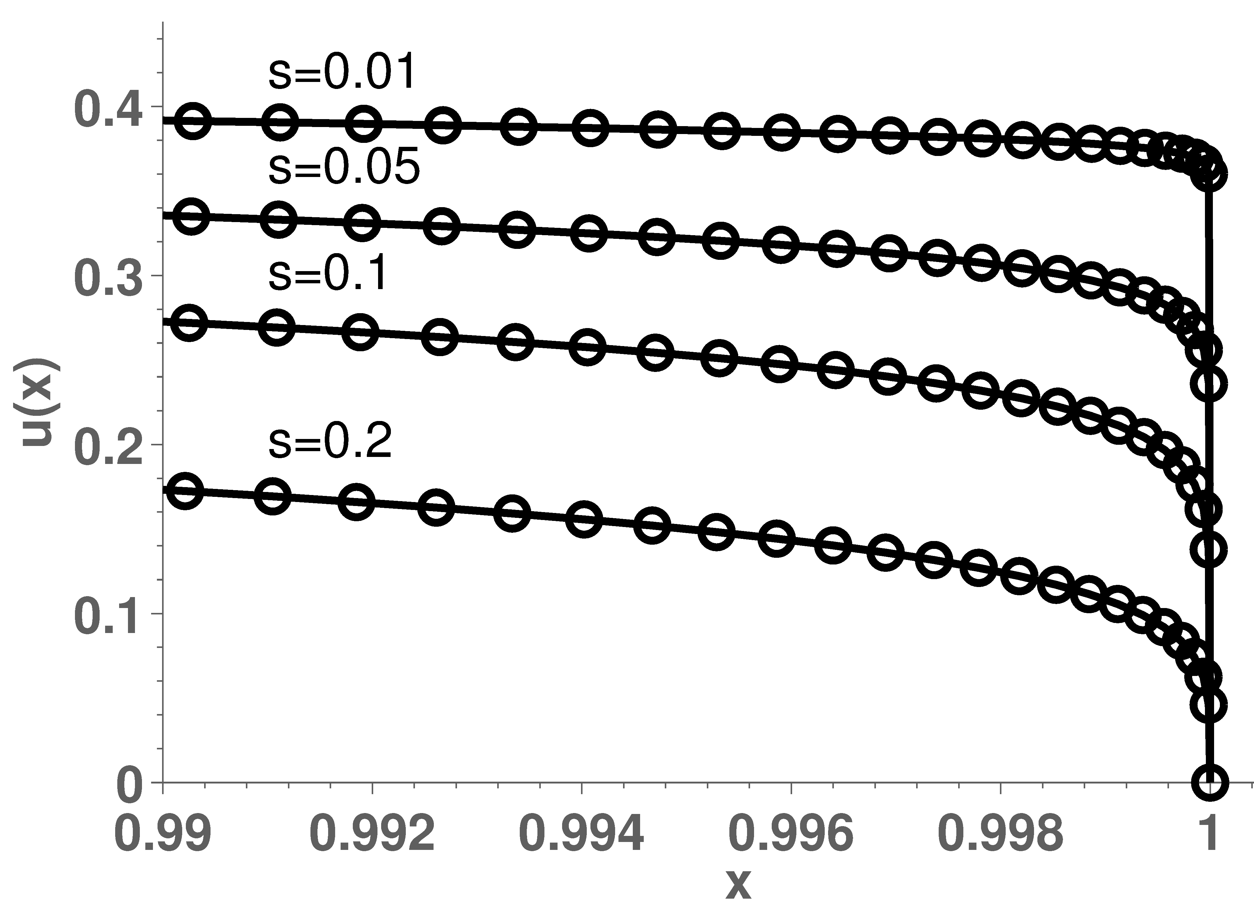
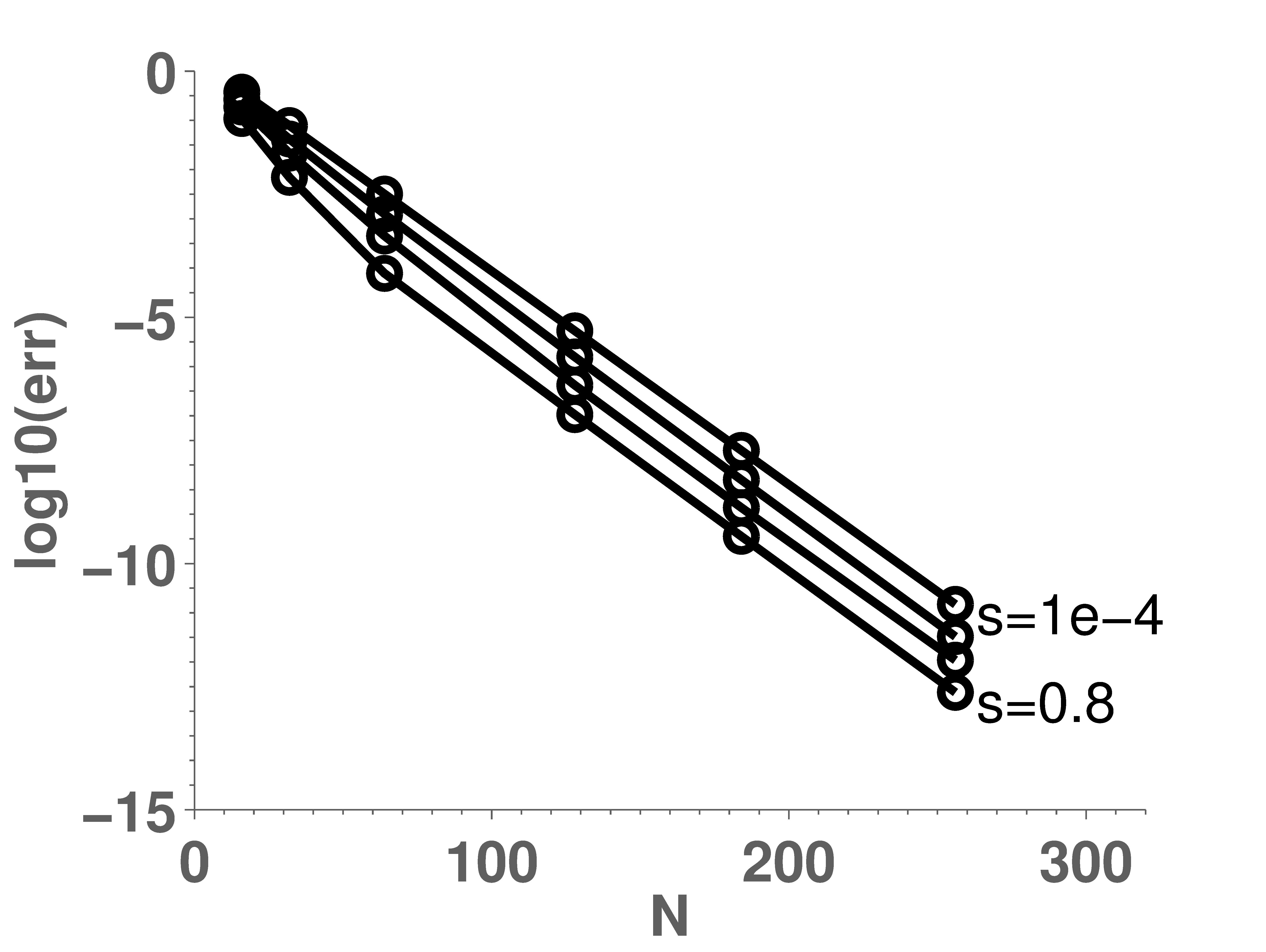
Figure 6.1. Exponential convergence for $f(x)=\frac{1}{x^{2}+0.01}$.

Left: Solution detail near the domain boundary for $f$ equal to the Runge function mentioned in the text. Right: Convergence for various values of $s$. Computation time: $0.0066$ sec. for $N=16$ to $0.05$ sec. for $N=256$.

Figure 6.1 demonstrates the exponentially fast convergence that takes place for a right-hand side given by the Runge function $f(x)=\frac{1}{x^{2}+0.01}$—which is analytic within a small region of the complex plane around the interval $[-1,1]$, and for values of $s$ as small as $10^{-4}$. The present Matlab implementation of our algorithms produces these solutions with near machine precision in computational times not exceeding $0.05$ seconds.

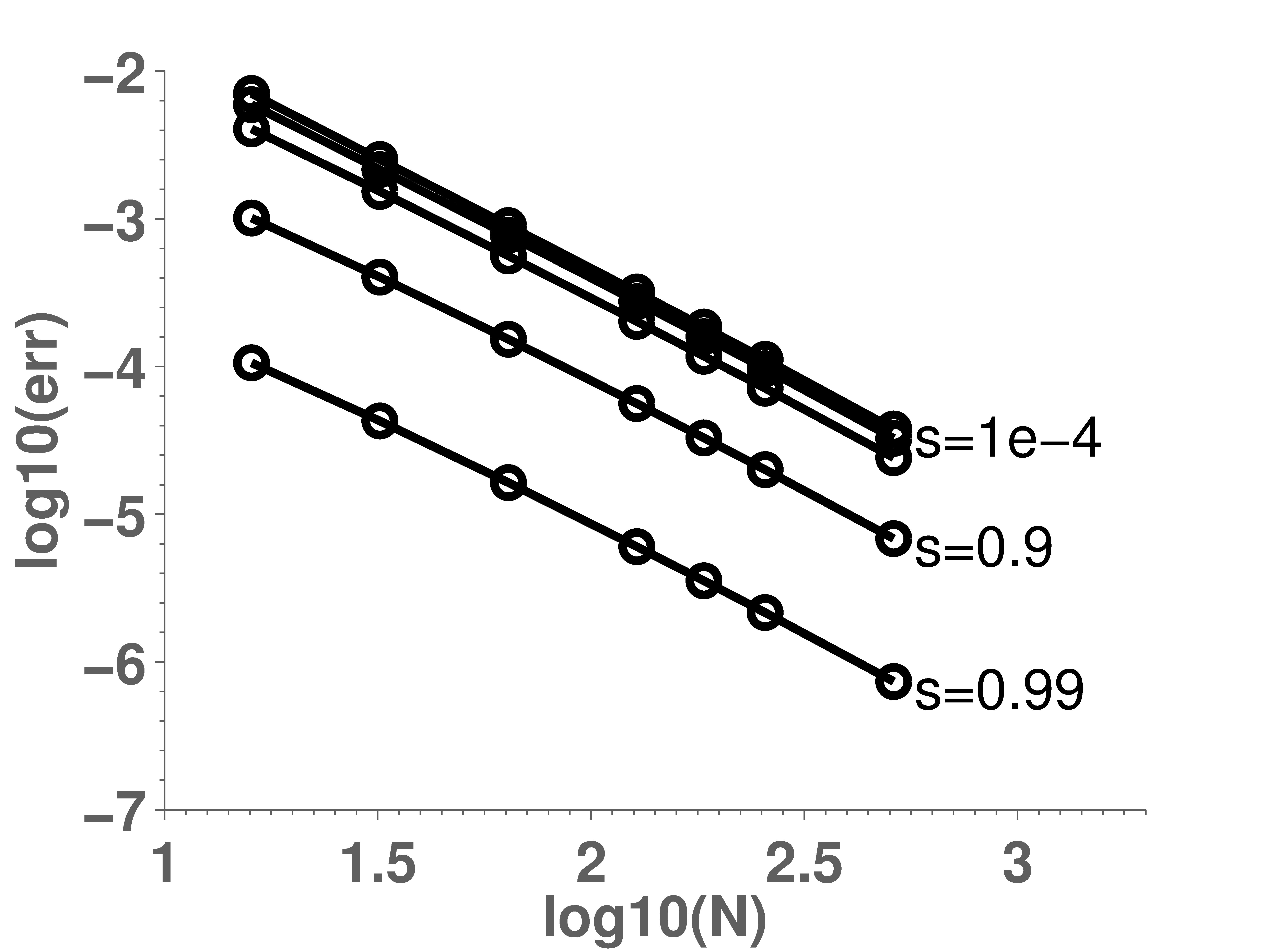
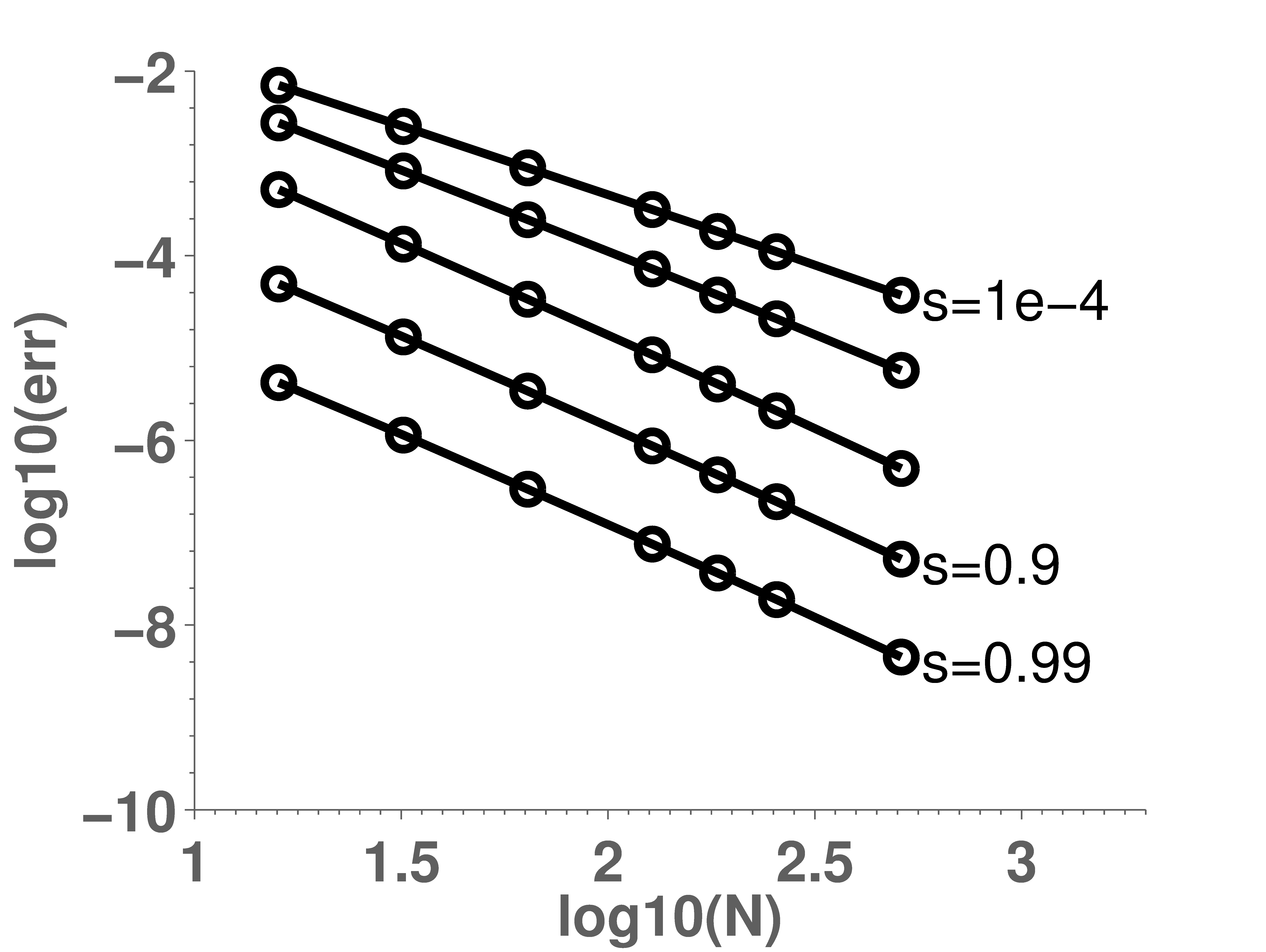
Figure 6.2. Convergence in the $H^{2s}_{s}(-1,1)$ and $L_{s}^{2}(-1,1)$ norms for $f(x)=|x|$. In this case, $f\in H^{3/2-\varepsilon}_{s}(-1,1)$.

Left: errors in $H^{2s}_{s}(-1,1)$ norm of order $1.5$. Right: errors in $L^{2}_{s}(-1,1)$ norm, orders range from $1.5$ to $2$.

Results concerning a problem containing the non-smooth right-hand side $f(x)=|x|$ (for which, as can be checked in view of Corollary 4.4 and Definition (4.6), we have $f\in H^{3/2-\varepsilon}_{s}(-1,1)$ for any $\varepsilon>0$ and any $0\leq s\leq 1$) are displayed in Fig. 6.2. The errors decay with the order predicted by Theorem 5.1 in the $H^{2s}_{s}(-1,1)$ norm, and with a slightly better order than predicted by that theorem for the $L_{s}^{2}(-1,1)$ error norm, although the observed orders tend to the predicted order as $s\to 0$ (cf. Remark 5.2).

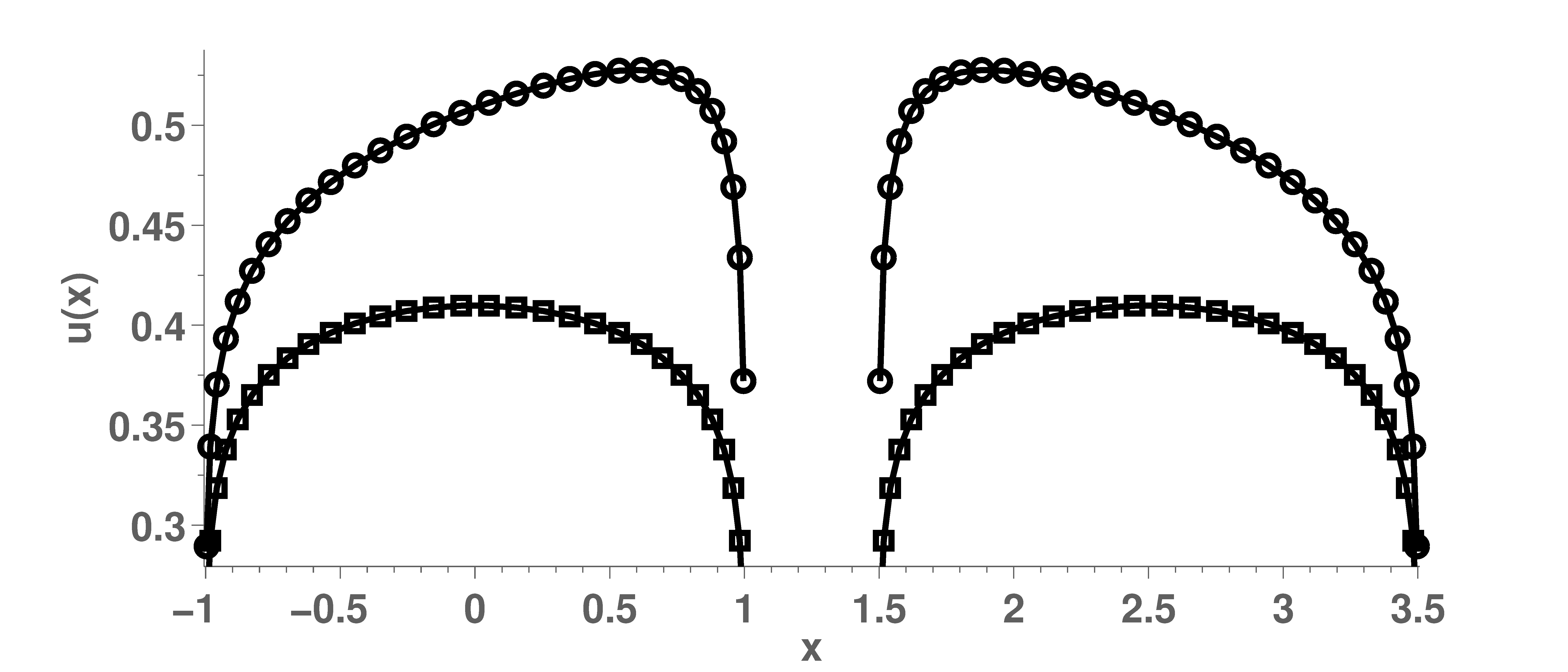
$N$	rel. err.
8	9.3134e-05
12	1.6865e-06
16	3.1795e-08
20	6.1375e-10
24	1.1857e-11
28	1.4699e-13

Figure 6.3. Multiple (upper curves) vs. independent single-intervals solutions (lower curves) with $f=1$. A total of five GMRES iterations sufficed to achieve the errors shown on the right table for each one of the discretizations considered.

A solution for a multi-interval (two-interval) test problem with right hand side $f=1$ is displayed in Figure 6.3. A total of five GMRES iterations sufficed to reach the errors displayed for each one of the discretizations considered on the right-hand table in Figure 6.3. The computational times required for each one of the discretizations listed on the right-hand table are of the order of a few hundredths of a second.

7. Acknowledgments

The authors thankfully acknowledge support from various agencies. GA work was partially supported by CONICET, Argentina, under grant PIP 2014–2016 11220130100184CO. JPB’s and MM’s efforts were made possible by graduate fellowship from CONICET, Argentina. OB efforts were supported by the US NSF and AFOSR through contracts DMS-1411876 and FA9550-15-1- 0043, and by the NSSEFF Vannevar Bush Fellowship under contract number N00014-16-1-2808.

Appendix A Appendix

A.1. Proof of Lemma 2.4

Let

$$F_{\varepsilon}(x)=\int_{\Omega\setminus B_{\varepsilon}(x)}\Phi_{s}(x-y)v(y)dy.$$

Then, by definition we have

$$\lim_{\varepsilon\to 0}\frac{d}{dx}F_{\varepsilon}(x)=P.V.\int_{\Omega}\frac{\partial}{\partial x}\Phi_{s}(x-y)v(y)dy.$$

We note that interchanging the limit and differentiation processes on the left hand side of this equation would result precisely in the right-hand side of equation (2.13)—and the lemma would thus follow. Since $F_{\varepsilon}$ converges throughout $\Omega$ as $\varepsilon\to 0$, to show that the order of the limit and differentiation can indeed be exchanged it suffices to show [33, Th. 7.17] that the quantity $\frac{d}{dx}F_{\varepsilon}(x)$ converges uniformly over compact subsets $K\subset\Omega$ as $\varepsilon\to 0$.

To establish the required uniform convergence property over a given compact set $K\subset\Omega$ let us first define a larger compact set $K^{*}=[a,b]\subset\Omega$ such that $K\subset U\subset K^{*}$ where $U$ is an open set. Letting $\varepsilon_{0}$ be sufficiently small so that $B_{\varepsilon_{0}}(x)\subset K^{*}$ for all $x\in K$, for each $\varepsilon<\varepsilon_{0}$ we may then write

$$\frac{\partial}{\partial x}F_{\varepsilon}=\int_{\Omega\setminus K^{*}}\frac{\partial}{\partial x}\Phi_{s}(x-y)v(y)dy+\int_{K^{*}\setminus B_{\varepsilon}(x)}\frac{\partial}{\partial x}\Phi_{s}(x-y)v(y)dy.$$

The first term on the right-hand side of this equation does not depend on $\varepsilon$ for all $x\in K$. To analyze the second term we consider the expansion $v(y)=v(x)+(y-x)R(x,y)$ and we write $\int_{K^{*}}\frac{\partial}{\partial x}\Phi_{s}(x-y)v(y)dy=\Gamma^{1}_{\varepsilon}(x)+\Gamma^{2}_{\varepsilon}(x)$ where

$$\begin{split}\Gamma^{1}_{\varepsilon}(x)&=v(x)\int_{K^{*}\setminus B_{\varepsilon}(x)}\frac{\partial}{\partial x}\Phi_{s}(x-y)dy\quad\mbox{and}\\ \Gamma^{2}_{\varepsilon}(x)&=\int_{K^{*}\setminus B_{\varepsilon}(x)}\frac{\partial}{\partial x}\Phi_{s}(x-y)(y-x)R(x,y)dy.\end{split}$$

Since $K^{*}=[a,b]$, for each $\varepsilon<\varepsilon_{0}$ and each $x\in K$ the quantity $\Gamma^{1}_{\varepsilon}(x)$ can be expressed in the form

$$\Gamma^{1}_{\varepsilon}(x)=-v(x)\left(\Phi_{s}(x-y)\big{|}^{y=b}_{y=x+\varepsilon}+\Phi_{s}(x-y)\big{|}^{y=x-\varepsilon}_{y=a}\,\right)$$

which, in view of the relation $\Phi_{s}(-\varepsilon)=\Phi_{s}(\varepsilon)$, is independent of $\varepsilon$. The uniform convergence of $\Gamma^{1}_{\varepsilon}(x)$ over $K$ therefore holds trivially.

The term $\Gamma^{2}_{\varepsilon}(x)$, finally, equals

$$\int_{K^{*}\setminus B_{\varepsilon}(x)}N(x-y)R(x,y),$$

where $N(x,y)=\frac{\partial}{\partial x}\Phi_{s}(x-y)(y-x)$. Since $v\in C^{1}(\Omega)$ there exists a constant $C_{K,K^{*}}$ such that $|R(x,y)|<C_{K,K^{*}}$ for all $(x,y)$ in the compact set $K\times K^{*}\subset\Omega\times\Omega$. In particular, for each $x\in K$ the product $N(x-y)R(x,y)$ is integrable over $K^{*}$, and therefore the difference between $\Gamma^{2}_{\varepsilon}(x)$ and its limit satisfies

$$\left|\Gamma^{2}_{\varepsilon}(x)-\lim_{\varepsilon\to 0}\Gamma^{2}_{\varepsilon}(x)\right|=\left|\int_{x-\varepsilon}^{x+\varepsilon}N(x-y)R(x,y)dy\right|<C_{K,K^{*}}\int_{-\varepsilon}^{\varepsilon}\left|N(z)\right|dz.$$

The uniform convergence of $\Gamma^{2}_{\varepsilon}$ over the set $K$ then follows from the integrability of the function $N=N(z)$ around the origin, and the proof is thus complete.

A.2. Interchange of infinite summation and P.V. integration in equation (3.23)

Lemma A.1.

Upon substitution of (3.22), the quantity $L^{s}_{n}$ in equation (3.19) equals the expression on the right-hand side of equation (3.23). In detail, for each $x\in(0,1)$ we have

(A.1) $$P.V.\int_{0}^{1}J^{s}(x-y)y^{s-1}\left(\sum_{j=0}^{\infty}q_{j}y^{j}\right)y^{n}dy=\sum_{j=0}^{\infty}\left(\mbox{P.V.}\int_{0}^{1}q_{j}y^{j}J^{s}(x-y)y^{s-1}y^{n}dy\right),$$

where $J^{s}(z)=\operatorname{sgn}(z)|z|^{-2s}$.

Proof.

Let $x\in(0,1)$ be given. Then, taking $\delta<\min\{x,1-x\}$ we re-express the left hand side of (A.1) in the form

(A.2) $$\lim_{\varepsilon\to 0}\left[\int_{0}^{\delta}dy+\int_{[\delta,1-\delta]\setminus B_{\varepsilon}(x)}dy+\int_{1-\delta}^{1}dy\right]\left(\sum_{j=0}^{\infty}J^{s}(x-y)q_{j}y^{s-1+n+j}\right).$$

The leftmost and rightmost integrals in this expression are independent of $\varepsilon$, and, in view of (3.22), they are both finite. The exchange of these integrals and the corresponding infinite sums follows easily in view of the monotone convergence theorem since the coefficients $q_{j}$ are all positive.

The middle integral in equation (A.2), in turn, can be expressed in the form

(A.3) $$\lim_{\varepsilon\to 0}\int_{[\delta,1-\delta]\setminus B_{\varepsilon}(x)}J^{s}(x-y)\left(\lim_{m\to\infty}v_{m}(y)\right)dy,$$

where

(A.4) $$v_{m}(y)=y^{s-1}y^{n}\sum_{j=0}^{m}q_{j}y^{j}.$$

In view of (3.22), $v_{m}$ converges (uniformly) to the smooth function $v_{\infty}(y)=y^{s-1}y^{n}(1-y)^{s-1}$ for all $y$ in the present domain of integration. As shown below, interchange of this uniformly convergent series with the PV integral will then allow us to complete the proof of the lemma.

In order to justify this interchange we replace the expansion

$$v_{m}(y)=v_{m}(x)+(x-y)R_{m}(x,y),\quad\mbox{where }R_{m}(x,y)=\frac{v_{m}(y)-v_{m}(x)}{x-y}.$$

in (A.3) and we define

(A.5) $$F^{1}_{\varepsilon}=v_{\infty}(x)\int_{[\delta,1-\delta]\setminus B_{\varepsilon}(x)}J^{s}(x-y)dy$$

(A.6) $$F^{2}_{\varepsilon}=\int_{[\delta,1-\delta]\setminus B_{\varepsilon}(x)}J^{s}(x-y)(x-y)\lim_{m\to\infty}R_{m}(x,y)dy;$$

clearly the expression in equation (A.3) equals $\lim_{\varepsilon\to 0}\left(F^{1}_{\varepsilon}+F^{2}_{\varepsilon}\right)$.

The exchange of $\lim_{\varepsilon\to 0}$ and infinite summation for $F^{1}_{\varepsilon}$ (in (A.5)) follows immediately since $v_{m}(x)$ does not depend on $\varepsilon$. In order to perform a similar exchange for $F^{2}_{\varepsilon}$ in (A.6) we first note that

(A.7) $$\lim_{\varepsilon\to 0}F^{2}_{\varepsilon}=\int_{\delta}^{1-\delta}J^{s}(x-y)(x-y)\lim_{m\to\infty}R_{m}(x,y)dy$$

in view of the integrand’s integrability—which itself follows from the bound

(A.8) $$\left|J^{s}(x-y)(x-y)\lim_{m\to\infty}R_{m}(x,y)\right|\leq M\left|J^{s}(x-y)(x-y)\right|,$$

(where $M$ is a bound for the derivative $\left[v_{\infty}(y)\right]^{\prime}$ in the interval $[\delta,1-\delta]$) together with the integrability of the product $\left|J^{s}(x-y)(x-y)\right|$. But (A.7) equals

(A.9) $$\begin{split}\lim_{m\to\infty}\int_{\delta}^{1-\delta}&J^{s}(x-y)(x-y)R_{m}(x,y)dy=\\ &=\lim_{m\to\infty}\lim_{\varepsilon\to 0}\int_{[\delta,1-\delta]\setminus B_{\varepsilon}(x)}J^{s}(x-y)(x-y)R_{m}(x,y)dy.\end{split}$$

Indeed, the first expression results from an application of the dominated convergence theorem—which is justified in view of (A.8) since $R_{m}(x,y)$ is an increasing sequence—while the second equality, which puts our integral in “principal value” form, follows directly in view of the integrand’s integrability.

The lemma now follows by substituting first $R_{m}(x,y)=(v_{m}(y)-v_{m}(y))/(x-y)$ and then equation (A.4) in the right-hand integral of equation (A.9) and combining the result with corresponding sums for $F^{1}_{\varepsilon}$ and for the leftmost and rightmost integrals in (A.2)—to produce the desired right-hand side in equation (A.1). The proof is now complete. ∎

A.3. Interchange of summation order in (3.25) for $x\in(0,1)$

Letting

$$a_{jk}=\frac{(1-s)_{j}}{j!}\frac{(2s)_{k}}{k!}\frac{1}{s-n-j+k}\,x^{k},$$

in order to show that the summation signs in (3.25) can be interchanged it suffices to show that the series $\sum_{j,k}a_{jk}$ is absolutely convergent. To do this we write

$$\sum_{j=0}^{\infty} |a_{jk}|=\frac{(2s)_{k}}{k!}\,x^{k}\sum_{j=0}^{\infty}\frac{(1-s)_{j}}{j!}\frac{1}{|s-n-j+k|}=$$

$$=\frac{(2s)_{k}}{k!}x^{k}\left(\sum_{j=0}^{k-n}\frac{(1-s)_{j}}{j!}\frac{1}{s-n-j+k}+\sum_{j=k-n+1}^{\infty}\frac{(1-s)_{j}}{j!}\frac{1}{-s+n+j-k}\right).$$

Since $\frac{(1-s)_{j}}{j!}\sim j^{-s}$ as $j\to\infty$ we obtain

$$\sum_{j=k-n+1}^{\infty}\frac{(1-s)_{j}}{j!}\frac{1}{-s+n+j-k}\leq C\sum_{j=k-n+1}^{\infty}\frac{j^{-s}}{-s+n+j-k}\leq C(s)$$

and, in view of the fact that, in particular, $\frac{(1-s)_{j}}{j!}$ is bounded,

$$\sum_{j=0}^{k-n}\frac{(1-s)_{j}}{j!}\frac{1}{s-n-j+k}\leq\sum_{\ell=0}^{k-n}\frac{1}{s+\ell}=\frac{1}{s}+\sum_{\ell=1}^{k-n}\frac{1}{s+\ell}.$$

It follows that

$$\sum_{k=0}^{\infty}\sum_{j=0}^{\infty}|a_{jk}|\leq\sum_{k=0}^{\infty}\frac{(2s)_{k}}{k!}\left(C(s)+\sum_{\ell=1}^{k-n}\frac{1}{\ell}\right)x^{k}$$

and, since $\frac{(2s)_{k}}{k!}\sim k^{2s-1}$ and $\sum_{\ell=1}^{k-n}\frac{1}{\ell}\sim\ln k$ as $k\to\infty$, the sum $\sum_{j,k}a_{jk}$ is absolutely convergent for every $x\in(0,1)$, as needed.

References

- [1] Nicola Abatangelo. Large -harmonic functions and boundary blow-up solutions for the fractional laplacian. Discrete and Continuous Dynamical Systems, 35(12):5555–5607, 2015.
- [2] M. Abramowitz and I. Stegun. Handbook of Mathematical Functions. Dover Publications, 1965.
- [3] Gabriel Acosta and Juan Pablo Borthagaray. A fractional Laplace equation: Regularity of solutions and finite element approximations. SIAM Journal on Numerical Analysis, 55(2):472–495, 2017.
- [4] Guglielmo Albanese, Alessio Fiscella, and Enrico Valdinoci. Gevrey regularity for integro-differential operators. Journal of Mathematical Analysis and Applications, 428(2):1225 – 1238, 2015.
- [5] Ivo Babuska and Benqi Guo. Direct and inverse approximation theorems for the p-version of the finite element method in the framework of weighted Besov spaces. part I: Approximability of functions in the weighted Besov spaces. SIAM Journal on Numerical Analysis, 39(5):1512–1538, 2002.
- [6] W.N. Bailey. Generalized Hypergeometric Series. Cambrigde University Press, 1935.
- [7] David A. Benson, Stephen W. Wheatcraft, and Mark M. Meerschaert. Application of a fractional advection-dispersion equation. Water Resources Research, 36(6):1403–1412, 2000.
- [8] Jöran Bergh and Jörgen Löfström. Interpolation spaces: an introduction. Springer-Verlag, Berlin, 1976.
- [9] C. Brändle, E. Colorado, A. de Pablo, and U. Sánchez. A concave-convex elliptic problem involving the fractional laplacian. Proceedings of the Royal Society of Edinburgh: Section A Mathematics, 143:39–71, 2 2013.
- [10] Susanne C. Brenner and L. Ridgway Scott. The mathematical theory of finite element methods, volume 15 of Texts in Applied Mathematics. Springer-Verlag, New York, 1994.
- [11] Oscar P. Bruno and Stéphane K. Lintner. Second-kind integral solvers for TE and TM problems of diffraction by open arcs. Radio Science, 47(6):n/a–n/a, 2012. RS6006.
- [12] Luis Caffarelli and Luis Silvestre. An extension problem related to the fractional Laplacian. Comm. Partial Differential Equations, 32(7-9):1245–1260, 2007.
- [13] Peter Carr, Hélyette Geman, Dilip B. Madan, and Marc Yor. The fine structure of asset returns: An empirical investigation. The Journal of Business, 75(2):305–332, 2002.
- [14] Rama Cont and Peter Tankov. Financial modelling with jump processes. Chapman & Hall/CRC Financial Mathematics Series. Chapman & Hall/CRC, Boca Raton, FL, 2004.
- [15] Matteo Cozzi. Interior regularity of solutions of non-local equations in sobolev and nikol’skii spaces. Annali di Matematica Pura ed Applicata (1923 -), pages 1–24, 2016.
- [16] Marta D’Elia and Max Gunzburger. The fractional laplacian operator on bounded domains as a special case of the nonlocal diffusion operator. Computers & Mathematics with Applications, 66(7):1245 – 1260, 2013.
- [17] Eleonora Di Nezza, Giampiero Palatucci, and Enrico Valdinoci. Hitchhiker’s guide to the fractional Sobolev spaces. Bull. Sci. Math., 136(5):521–573, 2012.
- [18] Bartłomiej Dyda, Alexey Kuznetsov, and Mateusz Kwaśnicki. Fractional Laplace operator and Meijer G-function. Constructive Approximation, pages 1–22, 2016.
- [19] Paolo Gatto and Jan S. Hesthaven. Numerical approximation of the fractional Laplacian via hp-finite elements, with an application to image denoising. Journal of Scientific Computing, 2014.
- [20] Guy Gilboa and Stanley Osher. Nonlocal operators with applications to image processing. Multiscale Model. Simul., 7(3):1005–1028, 2008.
- [21] Gerd Grubb. Fractional Laplacians on domains, a development of Hörmander’s theory of -transmission pseudodifferential operators. Advances in Mathematics, 268:478 – 528, 2015.
- [22] Ben-yu Guo and Li-lian Wang. Jacobi approximations in non-uniformly Jacobi-weighted Sobolev spaces. Journal of Approximation Theory, 128(1):1–41, 2004.
- [23] Nicholas Hale and Alex Townsend. Fast and accurate computation of Gauss–Legendre and Gauss–Jacobi quadrature nodes and weights. SIAM Journal on Scientific Computing, 35(2):A652–A674, 2013.
- [24] Yanghong Huang and Adam M. Oberman. Numerical methods for the fractional laplacian: A finite difference-quadrature approach. SIAM J. Numer. Anal., 52(6):3056–3084, 2014.
- [25] D.C.Handscomb J.C. Mason. Chevyshev Polynomials. Chapman & Hall CRC, 2003.
- [26] Joseph Klafter and Igor M. Sokolov. Anomalous diffusion spreads its wings. Physics world, 18(8):29, 2005.
- [27] Rainer Kress. Linear integral equations. Springer-Verlag, New York, 2014.
- [28] T. A. M. Langlands, B. I. Henry, and S. L. Wearne. Fractional cable equation models for anomalous electrodiffusion in nerve cells: Finite domain solutions. SIAM Journal on Applied Mathematics, 71(4):1168–1203, 2011.
- [29] Stéphane K. Lintner and Oscar P. Bruno. A generalized Calderón formula for open-arc diffraction problems: theoretical considerations. Proceedings of the Royal Society of Edinburgh, Section: A Mathematics, 145:331–364, 4 2015.
- [30] Ralf Metzler and Joseph Klafter. The restaurant at the end of the random walk: recent developments in the description of anomalous transport by fractional dynamics. J. Phys. A, 37(31):R161–R208, 2004.
- [31] Ricardo H. Nochetto, Enrique Otárola, and Abner J. Salgado. A PDE approach to fractional diffusion in general domains: A priori error analysis. Foundations of Computational Mathematics, pages 1–59, 2014.
- [32] Xavier Ros-Oton and Joaquim Serra. The Dirichlet problem for the fractional Laplacian: Regularity up to the boundary. Journal de Mathématiques Pures et Appliquées, 101(3):275 – 302, 2014.
- [33] Walter Rudin. Principles of mathematical analysis, volume 3. McGraw-Hill New York, 1964.
- [34] Youcef Saad and Martin H. Schultz. Gmres: A generalized minimal residual algorithm for solving nonsymmetric linear systems. SIAM Journal on Scientific and Statistical Computing, 7(3):856–869, 1986.
- [35] Raffaella Servadei and Enrico Valdinoci. On the spectrum of two different fractional operators. Proc. Roy. Soc. Edinburgh Sect. A, 144(4):831–855, 2014.
- [36] G. T. Symm. Integral equation methods in potential theory. ii. Proceedings of the Royal Society of London A: Mathematical, Physical and Engineering Sciences, 275(1360):33–46, 1963.
- [37] Gabor Szegö. Orthogonal polynomials, Fourth Edition. American Mathematical Society, Colloquium publications, 1975.
- [38] Enrico Valdinoci. From the long jump random walk to the fractional Laplacian. Bol. Soc. Esp. Mat. Apl. SMA, 49:33–44, 2009.
- [39] Ziqing Xie, Li-Lian Wang, and Xiaodan Zhao. On exponential convergence of Gegenbauer interpolation and spectral differentiation. Mathematics of Computation, 82(282):1017–1036, 2013.
- [40] Y. Yan and I.H. Sloan. On integral equations of the first kind with logarithmic kernels. J. Integral Equations Applications, 1(4):549–580, 12 1988.
- [41] Xiaodan Zhao, Li-Lian Wang, and Ziqing Xie. Sharp error bounds for Jacobi expansions and Gegenbauer–Gauss quadrature of analytic functions. SIAM Journal on Numerical Analysis, 51(3):1443–1469, 2013.