6.1 Thermodynamic limit of the pressure: proof of Theorem 2.1
Since we have already shown the lower bound (2.8) in section 2, to finish the proof of Theorem 2.1
it remains to obtain
|
|
|
(6.33) |
We split this proof into several lemmata. But first, we need some additional
definitions.
We define the set of all –invariant even states. Let be the set of
bijective maps from to which leaves invariant all
but finitely many elements. It is a group w.r.t. the composition. The condition
|
|
|
(6.34) |
defines a group homomorphism ,
uniquely. Here, stands for a spin up
or down . Then, let
|
|
|
|
|
|
|
|
|
|
be the set of all –invariant even states, where is the
set of all states on . The set is
weak∗–compact and convex. In particular, the set of extremal points of , denoted by , is not
empty.
Now, to fix the notation and for the reader convenience, we collect
well–known results about the so–called relative entropy, cf. [25, 40]. Let and be
two states on the local algebra , with being faithful. Define the relative entropy
|
|
|
where is the density matrix associated to the state with . The relative entropy is super–additive: for
any , , and for any even states respectively on , and , and faithful, we have
|
|
|
(6.35) |
For even states and , respectively on and with , the even state is the unique extension of and
on satisfying for all and all ,
|
|
|
The state is called the product of and . The product of even states
is an associative operation. In particular, products of even states can be
defined w.r.t. any countable set of subalgebras of with for .
Observe that the relative entropy becomes additive w.r.t. product states: if
, where and are two even states respectively on and , then (6.35) is satisfied with equality. The relative entropy is also
convex: for any states and
on , faithful, and for any
|
|
|
(6.36) |
Meanwhile
|
|
|
|
|
(6.37) |
|
|
|
|
|
for any . Note that the relative entropy makes sense in a
class of states on much larger than that of even states on (cf. [40]), but this is not needed here.
The condition
|
|
|
uniquely defines a homomorphism on called right–shift homomorphism. Any state on such that is called shift–invariant and we denote by the set of shift–invariant states on . An important class of shift–invariant states are product states obtained by “copying” some
even state of the one–site algebra on all other
sites, i.e.,
|
|
|
(6.38) |
Such product states are important and used below as reference states. More
generally, a state is –periodic with if . For each , the set of
all –periodic states from is denoted by
Let be any faithful even state on and let be any –periodic state on . It immediately follows from
super–additivity (6.35) that for any
|
|
|
In particular, the following limit exists
|
|
|
(6.39) |
and is the relative entropy density of w.r.t. the reference state . This functional has the following important properties:
Lemma 6.2 (Properties of the relative entropy density)
At any fixed , the relative entropy density functional is lower
weak∗–semicontinuous, i.e., for any faithful even state
and any , the set
|
|
|
is open w.r.t. the weak∗–topology. It is also affine, i.e., for any
faithful state and states
|
|
|
with
Proof: Without loss of generality, let . From the
second equality of (6.39),
|
|
|
As the maps are weak∗–continuous for each , it follows
that is the union of open sets, which implies the
lower weak∗–semicontinuity of the
relative entropy density functional. Moreover
from (6.36) and (6.37) we directly obtain
that is affine.
Notice that any p.i. state is automatically shift–invariant. Thus, the mean
relative entropy density is a well–defined functional on . Now, we need to define on the functional relating to the mean BCS interaction energy
per site:
Lemma 6.3 (BCS energy per site for p.i. states)
For any , the mean BCS interaction energy
per site in the thermodynamic limit
|
|
|
|
|
|
|
|
|
|
is well–defined and the affine map , is weak∗–continuous.
Proof: First,
|
|
|
|
|
|
|
|
|
|
Since , for any observe that
|
|
|
(6.41) |
whereas
|
|
|
(6.42) |
Therefore, by combining (LABEL:BCS_equation_1) with (6.41)
and (6.42), the lemma follows.
Now, we define by
|
|
|
(6.43) |
the Gibbs state associated with any self–adjoint element of at inverse temperature . This definition is of course
in accordance with the Gibbs state (1.6)
associated with the Hamiltonian (1.2) since for any . Note however, that
the state is seen either as defined on the local algebra or as defined on the whole algebra by
periodically extending it (with period ).
Next we give an important property of Gibbs states (6.43):
Lemma 6.4 (Passivity of Gibbs states)
Let , be self–adjoint elements from
and define for any state on
|
|
|
where for
any self–adjoint . Then for any state on
with equality if . Note that is the free energy associated with the state .
Proof: For any self–adjoint
and any state on observe that
|
|
|
(6.44) |
which implies that
|
|
|
|
|
(6.45) |
|
|
|
|
|
i.e., . Without loss of
generality take any faithful state on . In
this case, there are positive numbers with and vectors from the Hilbert space such that . In particular, from (6.44) we have
|
|
|
Consequently, by convexity of the exponential function combined with Jensen
inequality we obtain that
|
|
|
|
|
|
|
|
|
|
|
|
|
|
|
Note that the last inequality uses the so–called Peierls–Bogoliubov
inequality which is again a consequence of Jensen inequality.
This proof is standard (see, e.g., [25]). It is only
given in detail here, because we also need later equations (6.44) and (6.45).
Observe that Lemma 6.4 applied to
gives the Bogoliubov (convexity) inequality [29]. We can
also deduce from this lemma that the pressure (1.4) associated with equals
|
|
|
|
|
(6.46) |
|
|
|
|
|
for any and real numbers Recall that is the shift–invariant state obtained by
“copying” the state
(6.32) of the one–site algebra , see (6.38).
Lemma 6.5 (From to the relative entropy density at finite
)
Let be the shift–invariant state defined by
|
|
|
where is the right–shift homomorphism. Then , cf. (6.39).
Proof: By Lemma 6.2 combined
with (6.39), the relative entropy density equals
|
|
|
(6.47) |
for any fixed . By using now the additivity of the relative
entropy for product states observe that
|
|
|
|
|
(6.48) |
|
|
|
|
|
for any with by definition. Therefore the equality directly follows from (6.47) combined with (6.48).
We are now in position to give a first general upper bound for the pressure by using the
equality (6.46) together with Lemmata 6.3 and 6.5.
Lemma 6.6 (General upper bound of the pressure )
For any and , one gets
that
|
|
|
where we recall that is the non empty set
of extremal points of .
Proof: By (6.46) combined with Lemma 6.5 one gets
|
|
|
|
|
(6.49) |
|
|
|
|
|
The last term of this equality is independent of since
|
|
|
(6.50) |
cf. (2.9).
However, the other terms require the knowledge of the states
and in the limit . Actually,
because the unit ball in is a metric space w.r.t. the
weak∗–topology, the sequence converges in the
weak∗–topology along a subsequence towards .
Meanwhile, it is easy to see that for all , ,
|
|
|
Thus, the sequences of states and have
the same limit points. Since is even and permutation invariant
w.r.t. the first sites, the state belongs to . We now estimate the first term (6.49)
as in Lemma 6.3 to get
|
|
|
|
|
(6.51) |
|
|
|
|
|
From Lemma 6.2 the relative entropy density is
lower semicontinuous in the weak∗–topology, which implies that
|
|
|
By combining this last inequality with (6.51) we then find
that
|
|
|
(6.52) |
with
Now, from Lemma 6.3 the functional is affine and weak∗–continuous, whereas by Lemma 6.2 the map is affine and lower weak∗–semicontinuous. The free
energy functional is, in particular, convex and
upper weak∗–semicontinuous. Meanwhile recall that is a
weak∗–compact and convex set. Therefore, from the Bauer maximum
principle [32, Lemma 4.1.12] it follows that
|
|
|
(6.53) |
Together with (6.52), this last inequality implies the
upper bound stated in the lemma.
Since even states on are entirely determined by their action
on even elements from , observe that we can identify the set of
even p.i. states of with the set of p.i. states on the even
sub–algebra . We want to show next that the set of
extremal points belongs to the set of
strongly clustering states on the even sub–algebra of . By strongly clustering states w.r.t. , we mean that for any in , there exists a net such that for any ,
|
|
|
uniformly in . Here, denotes the convex hull of
the set .
Lemma 6.7 (Characterization of the set of extremal states of )
Any extremal state is strongly
clustering w.r.t. the even sub–algebra and conversely.
Proof: We use some standard facts about extremal
decompositions of states which can be found in [32, Theorems 4.3.17 and
4.3.22]. To satisfy the requirements of these theorems,
we need to prove that the –algebra of even
elements of is asymptotically abelian w.r.t. the action of the
group . This is proven as follows. For each define the
map by
|
|
|
(6.54) |
In other words, the map exchanges the block with and leaves the rest
invariant. For any with , it is then not difficult to see that
|
|
|
in the norm sense. Recall that the map is defined via (6.34). By density of local elements of the
limit above equals zero for all . Therefore, by
using now [32, Theorems 4.3.17 and 4.3.22] all states are then strongly clustering
w.r.t. and conversely.
We show next that p.i. states, which are strongly clustering w.r.t. the even
sub–algebra have clustering properties w.r.t. the whole
algebra .
Lemma 6.8 (Extension of the strongly clustering property)
Let be any strongly clustering state
w.r.t. . Then, for any and , there are and such that for any ,
|
|
|
Proof: By density of local elements it suffices to prove
the lemma for any and . The
operators and can always be written as sums and , where and are in the even sub–algebra whereas and are odd elements, i.e., they
are sums of monomials of odd degree in annihilation and creation operators.
Since is assumed to be strongly clustering w.r.t. , for any there are positive numbers with and maps such that for any ,
|
|
|
(6.55) |
By parity and linearity of observe that , whereas
|
|
|
(6.56) |
for large enough with the operator defined by
|
|
|
(6.57) |
The equality (6.56) follows from parity and the statement
|
|
|
for any , odd, and sufficiently large . This can be seen as
follows. Since any element of with defined parity can be
written as a linear combination of two self–adjoint elements with same
parity, we assume without loss of generality that . Choose large enough such that
the support of does not
intersect for all . The
map is defined by (6.54). Define , , where is
the right–shift homomorphism. For any
|
|
|
by symmetry of . Use now the Cauchy–Schwarz inequality for states
to get
|
|
|
Since per construction, and anti–commute if ,
|
|
|
By symmetry of , the right–hand side of the equation above equals . Hence, we conclude that
|
|
|
for any , i.e., for all .
Therefore, the lemma follows from (6.55)–(6.56) with defined by (6.57) for any .
We now identify the set of clustering states on with the set
of product states by the following lemma, which is a non–commutative
version of de Finetti Theorem of probability theory [28]. Størmer [1] was the first to show the corresponding result for
infinite tensor products of –algebras.
Lemma 6.9 (Strongly clustering p.i. states are product states)
Any p.i. and strongly clustering (in the sense of Lemma 6.8)
state is a product state (6.38)
with the one–site state being the restriction of on the local (one–site) algebra .
Proof: Let with whenever , and for any take
. To prove the lemma we need to show that
|
|
|
(6.58) |
The proof of this last equality for any is performed by induction.
First, for the equality (6.58) immediately follows
by symmetry of the state . Now, assume the equality (6.58) verified at fixed The state is strongly
clustering in the sense of Lemma 6.8. Therefore for each there are , positive numbers with and
maps such that
|
|
|
(6.59) |
for any . Fix sufficiently large such that the
operators and belong to for any and . We
can choose sufficiently large such that for
any , which by symmetry of
implies that
|
|
|
|
|
|
|
|
|
|
Combined with (6.59) and it yields
|
|
|
Since the equality (6.58) is assumed to be verified at
fixed it follows that
|
|
|
for any . In other words, by induction the equality (6.58) is proven for any
As soon as the upper bound is concerned, we combine Lemma 6.6
with Lemmata 6.7–6.9 to obtain that
|
|
|
(6.60) |
Here denotes the set of even states on the
(one–site) algebra . Now the proof of the upper bound (6.33) easily follows from the passivity of Gibbs states
on . Indeed, we apply Lemma 6.4 to the
one–site Hamiltonians (see (2.7)) and
|
|
|
in order to bound the relative entropy .
More precisely, it follows that
|
|
|
|
|
(6.61) |
|
|
|
|
|
for any state and any
with and Consequently,
from (6.60) we deduce that
|
|
|
|
|
|
|
|
|
|
|
|
|
|
|
|
|
|
|
|
|
|
|
|
|
In particular, by fixing and in the infimum we
finally obtain
|
|
|
i.e., the upper bound (6.33) for any and
6.2 Equilibrium and ground states of the strong coupling BCS-Hubbard
model
It follows immediately from the passivity of Gibbs states that
|
|
|
(6.62) |
for any , cf. (6.32) and
Lemmata 6.3–6.4. Therefore, by using Lemma 6.6 with (6.53) the (infinite volume)
pressure can be written as
|
|
|
Moreover, as shown above (see the upper bound in the proof of Lemma 6.6), any weak∗ limit point of local Gibbs
states (1.6) when
satisfies (6.62) with equality.
Indeed, by using (6.44) one obtains for any state
that
|
|
|
|
|
(6.63) |
|
|
|
|
|
|
|
|
|
|
with being the (finite volume) pressure (1.4) associated with the Hamiltonian (1.2), being the product state
obtained by “copying” the state (6.32) on the one–site algebra (see (6.38)), and with the trace state
defined on the local algebra for by
|
|
|
For any permutation invariant state it is straightforward to check
that the limits
|
|
|
and
|
|
|
exist for any fixed parameters and , see respectively (2.7) and
Lemma 6.3 for the definitions of and . Combined with (6.50) and (6.63) it then follows that the usual entropy density
|
|
|
|
|
|
|
|
|
|
of the permutation invariant state also exists and
|
|
|
The set of equilibrium states of the strong coupling
BCS–Hubbard model is defined by
|
|
|
|
|
|
|
|
|
|
Note that contains per construction all
weak∗ limit points of local Gibbs states as .
Consequently, the equilibrium states are, as usual, the minimizers of the
free energy functional
|
|
|
(6.64) |
on the convex and weak∗–compact set , cf. (1.5). They also maximize the upper semicontinuous affine functional It follows that is a closed face
of and we have in this set a notion of pure and
mixed thermodynamic phases (equilibrium states) by identifying purity with
extremality. In particular, it is convex and weak∗–compact. Each
weak∗–limit of equilibrium states such
that and is called a ground
state of the strong coupling BCS–Hubbard model. The set of all ground
states with parameters and is
denoted by . Extremal states of the weak∗–compact convex
set are called pure ground states.
We analyze now the set of pure equilibrium states, i.e., the equilibrium
states belonging to the set of extremal points of , cf. (6.53). First, from Lemmata 6.7–6.9 recall that any extremal state is a product state (6.38), i.e., it is obtained by
“copying” a state on the
one–site algebra to the other sites. In particular, by
combining (6.53) with (6.62)
observe that
|
|
|
(6.65) |
Therefore, a product state is a pure equilibrium state if
and only if belongs to the set of one–site equilibrium states defined
by
|
|
|
(6.66) |
In other words, the study of pure states of can
be reduced, without loss of generality, to the analysis of The first important statement concerns the characterization of
the set in relation with the variational problems (2.10) and (6.65).
Theorem 6.10 (Explicit description of one-site equilibrium states)
For any and , the set of one–site equilibrium states are given by the
states (6.32) with for any order
parameter solution of (2.10) and any
phase .
Proof: Take any solution of (2.10) and any . Then, from (6.45) observe that
|
|
|
(6.67) |
Since and the last
equality combined with Theorem 2.1 implies that
|
|
|
(6.68) |
In other words, is a maximizer of
the variational problem defined in (6.65) and hence, .
On the other hand, any state satisfies (6.68) and by combining Theorem 2.1 with
the inequality (6.61) for it follows that
|
|
|
Hence, for some .
It remains to prove that the equality uniquely defines the one–site equilibrium state . It follows from with that and
|
|
|
(6.69) |
because of (6.67), see (2.7) for the definition of . By Lemma 6.4, one obtains for any self–adjoint
that
|
|
|
(6.70) |
Consequently, we obtain by combining (6.69) and (6.70) that
|
|
|
for any self–adjoint and such that . In other words, the functional is tangent to the pressure
at . Since the convex map is continuously differentiable and self–adjoint
elements separate states, the tangent functional is unique and .
It follows immediately from the theorem above that pure states of solve the gap equation:
Corollary 6.11 (Gap equation for pure equilibrium states)
For any and , pure states
from are precisely the product states satisfying the gap equation for any and with being any
maximizer of the first variational problem given in Theorem 2.1.
If observe that the gap equation with defined in
(6.32) corresponds to the Euler–Lagrange equation satisfied
by the solutions
of the first variational problem given in Theorem 2.1. The
phase is arbitrarily taken because of the gauge
invariance of the map , and the gap equation can be reduced to (2.11). In other words, if , the gap equation
can be written in two different ways: either in the view point of extremal equilibrium states or (2.11) in the view point of the order parameter .
From this last corollary observe also that the existence of non–zero
maximizers implies the existence of equilibrium
states breaking the –gauge symmetry satisfied by (1.2). This breakdown of the –gauge symmetry
for is already explained by Theorem 3.3, which can be proven by our notion of equilibrium states as
follows.
Consider the upper semicontinuous convex map on
defined for any and by
|
|
|
(6.71) |
From Section 6.1 it is straightforward to check that
|
|
|
|
|
|
|
|
|
|
with the Hamiltonian defined in (3.14). Moreover, any weak∗–limits of local Gibbs states
|
|
|
(6.73) |
are equilibrium states (see the proof of Lemma 6.6 applied to ), i.e., the state belongs to the (non-empty) convex set of maximizers of (6.71) at fixed
and . In fact, one gets the following statement,
which implies Theorem 3.3.
Theorem 6.12 (Breakdown of the -gauge symmetry)
Take and real numbers away from any
critical point. Then at fixed phase ,
|
|
|
with being the unique maximizer of (6.71) for
sufficiently small .
Proof: First we need to characterize pure states of as it is done in Corollary 6.11 for By convexity and upper
semicontinuity, note that maximizers of (6.71) are
taken on the set of extremal states whereas the set of extremal maximizers
is a face. Since extremal states are product states (cf. Lemma 6.7-6.9), we get that
|
|
|
|
|
(6.74) |
|
|
|
|
|
as in the case (see (2.9) for the
definition of ). If is a
maximizer of
|
|
|
(6.75) |
then observe that maximizes the function
|
|
|
of the complex variable . By gauge invariance of the map , it follows that and thus . Using this, we extend Corollary 6.11 to and . In other words, for any , , and , pure states
of are product states satisfying the gap
equation
|
|
|
(6.76) |
for any and with being any maximizer of (6.75).
As , notice that . So, by gauge invariance we obtain
|
|
|
|
|
|
|
|
|
|
for any and sufficiently large. Consequently,
if the parameters and are such
that the maximizer (2.10) is unique,
then the maximizer of (6.75) is also unique as soon as is
sufficiently small. Indeed the map is
continuous on the compact interval In particular, from (6.76) there is a unique maximizer of (6.71), i.e.,
|
|
|
(6.77) |
Moreover, converges to as . Therefore, it follows
from (6.76) that
|
|
|
(6.78) |
for any .
By permutation invariance
|
|
|
Now, let and be two subsequences in such that
|
|
|
|
|
|
|
|
|
|
We can assume without loss of generality that and both converge w.r.t. the weak∗–topology as . Since any weak∗–limits of local Gibbs states (6.73) are equilibrium states (see again the proof
of Lemma 6.6), i.e., , the theorem then follows from (6.77) and (6.78).
Indeed, for any and
away from any critical point, the sequence of
local Gibbs state converges towards in the
weak∗–topology as soon as
is sufficiently small.
From Corollary 6.11 note that the expectation
values of Cooper fields
|
|
|
(6.79) |
are
|
|
|
(6.80) |
for any pure state of and , where we recall that is some maximizer
of the first variational problem given in Theorem 2.1. In
particular, or for any pure state is a
manifestation of the breakdown of the –gauge symmetry.
Unfortunately, the operators and
do not correspond to any experiment, as they are not gauge invariant. More
generally, experiments only “see” the
restriction of states to
the subalgebra of gauge invariant elements. Consequently, the next step is
to prove the so–called off diagonal long range order (ODLRO)
property proposed by Yang [38] to define the superconducting phase.
Indeed, one detects the presence of –gauge symmetry breaking by
considering the asymptotics, as , of the (–gauge symmetric) Cooper pair correlation function
|
|
|
(6.81) |
associated with some state . In particular, if
converges to some fixed non–zero value whenever ,
the state shows off diagonal long range order (ODLRO).
This property can directly be analyzed for equilibrium states from our next
statement.
Theorem 6.13 (Cooper pair correlation function)
For any and away from any
critical point, the Cooper pair correlation function
associated with the local Gibbs state converges for fixed towards
|
|
|
for any equilibrium state , and with being the solution of (2.10).
Proof: By similar arguments as in the proof of Theorem 6.12, if for all equilibrium states , then
|
|
|
By permutation invariance of , note
that
|
|
|
(6.82) |
for any If is an extremal equilibrium state, then one clearly has
|
|
|
On the other hand, the set of equilibrium states
for fixed parameters , and
is weak∗–compact. In particular, if is not extremal, the function is given, up to
arbitrarily small errors, by convex sums of the form
|
|
|
(6.83) |
where are extremal equilibrium states. Since
any weak∗–limit of local Gibbs states (1.6) is an equilibrium state (see proof of Lemma 6.6), the theorem is then a consequence of (6.82)–(6.83).
Since
|
|
|
|
|
|
|
|
|
|
note that this theorem implies Theorem 3.1.
Therefore, away from any critical point, if an equilibrium state shows ODLRO
then all pure equilibrium states break the –gauge symmetry.
Conversely, if all pure equilibrium states break the –gauge symmetry,
then all equilibrium state show ODLRO. This is due to the fact that the
order parameter is unique away from any critical point.
In particular, from Section 7, at
sufficiently small inverse temperature there is no ODLRO and , whereas for
sufficiently large and all equilibrium states show ODLRO.
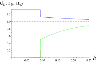
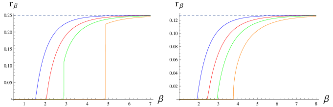
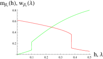
For any and real numbers at some
critical point, this property is not satisfied in general. There are indeed
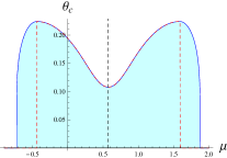
cases where the phase transition is of first order, cf. figure 3. In this situation, and some are maximizers at the same time, and hence, there are some
equilibrium states breaking the –gauge symmetry and other equilibrium
states which do not show ODLRO in this specific situation.
Observe now that the superconducting phase is not only characterized by
ODLRO and the breakdown of the –gauge symmetry. Indeed, the
two–point correlation function determines its type: s–wave, d–wave,
p–wave, etc. In fact, for any extremal equilibrium state , and , one clearly has
|
|
|
As a consequence, for any equilibrium state , we have and we obtain a s–wave
superconducting phase. In particular, Theorem 3.4 is a
simple consequence of this last equalities combined with (6.77), (6.78) and the fact
that any weak∗–limits of local Gibbs states (6.73) are equilibrium states (see
again the proof of Lemma 6.6).
Now we would like to pursue this analysis of equilibrium states by showing
that their definition is in accordance with results of Theorems 3.8, 3.10 and 3.12. This
statement is given in the next theorem.
Theorem 6.14 (Uniqueness of densities for equilibrium states)
Take and real numbers away from any
critical point. Then, for any equilibrium state and all densities are uniquely defined:
(i) The electron density is equal to
|
|
|
cf. Theorem 3.8.
(ii) The magnetization density is equal to
|
|
|
cf. Theorem 3.10.
(iii) The Coulomb correlation density is equal to
|
|
|
cf. Theorem 3.12.
Proof: Suppose first that is pure. Then, from Corollary 6.11
it follows that
|
|
|
with for some . Thus, by using the gauge invariance of the map we directly get
|
|
|
(6.84) |
At fixed parameters , ,
recall that the set of equilibrium states is
weak∗–compact. In particular, if is not pure, it is the weak∗–limit of convex combinations of pure
states. Therefore, we obtain (6.84) for any Similarly one gets
|
|
|
(6.85) |
for any equilibrium state and . Moreover, since any weak∗–limit of
local Gibbs states (1.6) is an
equilibrium state, i.e., ,
we therefore deduce from (6.84)-(6.85),
exactly as in the proof of Theorem 6.12, the existence of the limits in the statements (i)-(iii).
Observe that the weak∗–limit of local Gibbs states (1.6)
can easily be performed, even at critical points, by using the
decomposition theory for states [32]:
Theorem 6.15 (Asymptotics of the local Gibbs state
as )
Recall that for any , is a maximizer of the first variational
problem given in Theorem 2.1, whereas the states and are respectively defined by (6.32) and (6.38). Take any , , and let .
(i) Away From any critical point, the local Gibbs state
converges in the weak∗–topology towards the equilibrium state
|
|
|
(6.86) |
(ii) For each weak∗ limit point of local Gibbs
states with parameters converging to any critical point (2.13),
there is such that
|
|
|
Proof: By –gauge symmetry of the Hamiltonians (1.2) recall that any
weak∗–limit of local Gibbs states (1.6) is a –invariant equilibrium state. So, in order to
prove the first part of the Theorem it suffices to show that the equilibrium
state given in (i) is the unique –invariant state in . If the solution of (2.10)
is zero, then this follows immediately from Corollary 6.11.
Let be the unique maximizer of (2.10), i.e.,
for any . Let
|
|
|
be the set of all extremal states of , see (6.66) for the definition of the set of one–site equilibrium states. Observe that the
closed convex hull of is precisely and that is
the image of the torus under the continuous map , with . This last map defines a homeomorphism
between the torus and . In particular,
the set is compact and for each
equilibrium state there is a uniquely
defined probability measure on the
torus such that
|
|
|
(6.87) |
See, e.g., Proposition 1.2 of [41]. By –invariance of , for any one has from (6.87) that
|
|
|
Therefore, if there is a unique probability measure
allowing the –gauge symmetry of : must be the
uniform probability measure on .
From Lemma 7.1 the cardinality of set of maximizers of (2.10) is at most . Indeed, away from any critical point, it
is whereas at a critical point it can be either (second order phase
transition) or (first order phase transition). For more details, see
Section 7. In both cases, we can use the
same arguments as above. By similar estimates as in the proof of Lemma 6.6 it immediately follows that all limit points of the Gibbs
states with parameters converging to as , belongs to . Since the set
of all –invariant equilibrium states from
is for any with
|
|
|
(6.88) |
we obtain the second statement (ii).
This theorem is a generalization of results obtained for the strong coupling BCS model
[7]. Note however, that Thirring’s analysis [7] of the
asymptotics of local Gibbs states comes from explicit computations, whereas
we use the structure of sets of states, as explained for instance in [33].
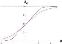
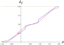
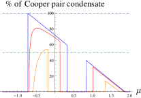
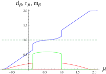
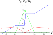
Observe that Theorem 4.3 is a simple consequence of Theorem 6.15. Indeed, assume for instance that the
order parameter and the electron density per site jumps respectively from to and from to by crossing a critical chemical
potential at fixed parameters . An example of such behavior is given in figure 10 for an electron density smaller than one. If , then the
unique solution
of (4.29) must converge towards as . Meanwhile, at fixed
|
|
|
with and
Any weak∗–limit of
local Gibbs states satisfies per construction
|
|
|
and has the form (6.88), by Theorem 6.15.
Hence, the Gibbs state converges in the weak∗–topology
towards with
defined in Theorem 4.3. Indeed, the existence of the limits
(i)–(iii) in Theorem 4.3 follows from the uniqueness of the
limiting equilibrium state with fixed electron density .
We give now various important properties of densities in ground states,
i.e., for , which immediately follow from Theorem 6.14. Recall that the set of ground states is the set of all weak∗ limit points as of all equilibrium state sequences with diverging inverse temperature .
Take and parameters such that . Then the electron and Coulomb correlation densities
equal respectively
|
|
|
(6.89) |
for any ground state and , cf. Corollaries 3.9 and 3.13.
If additionally , we are in
the superconducting phase for ground states, cf. Corollary 3.5. Indeed, for any , there is a ground
state such that for any ,
|
|
|
In the superconducting phase, from Corollary 3.13 we
observe that , whereas the
magnetization density equals
|
|
|
(6.90) |
for any superconducting state and . This is the Meißner effect, see Corollary 3.11. On the other hand, the Cauchy–Schwarz inequality for the
states implies the inequalities
|
|
|
(6.91) |
for any and . In fact, in
the superconducting phase the second inequality of (6.91) is an
equality for any . Indeed, (6.90) and Corollary 3.13 yield
|
|
|
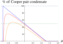
(6.92) |
for any and . It
shows that 100% of electrons form Cooper pairs in superconducting ground
states.
In the case where with and , the density vector defined by (6.89) and (6.90) is also unique as in the superconducting phase. It
equals ,
see Corollaries 3.9, 3.11 and 3.13. However, if with , or , or , then the density vector belongs, in general, to a non trivial convex set. In other
words, there are phase transitions involving to these densities. In
particular, even in the case where the Hamiltonian (1.2) is spin invariant, there are ground states
breaking the spin –symmetry.
For instance, take and parameters such
that and . Then for any and , the electron density equals , whereas the Coulomb correlation density is . In particular, the first inequality of (6.91) is an
equality showing that 0% of electrons forms Cooper pairs. But, even if
the magnetic field vanishes, i.e., for any there exists
a ground state
with magnetization density (see (6.90) for
the definition of ).
Therefore, all the thermodynamics of the strong coupling BCS–Hubbard model
discussed in Sections 3.1–3.5 is encoded in the notion of equilibrium and ground states with . However, there
is still an important open question related to the thermodynamics of this
model. It concerns the problem of fluctuations of the Cooper pair condensate
density (Theorem 3.1) or Cooper fields
and (6.79) as a function of the
temperature. Unfortunately, no result in that direction are known as soon as
the thermodynamic limit is concerned. We prove however a simple statement
about fluctuations of Cooper fields for pure states from in the limit .
Theorem 6.16 (Fluctuations of Cooper fields)
Take and real numbers away from any
critical point. Then, for any pure state and , the
fluctuations of Cooper fields and (6.79) are bounded by
|
|
|
i.e., they vanish in the limit .
Proof: Recall that properties of pure states are
characterized in Corollary 6.11, i.e., they are
product states with the
one–site state being defined in (6.32). In particular, they satisfy (6.80). Now, to avoid triviality, assume that and let be
the function defined for any by
|
|
|
Since is a maximizer of the function of , one has , i.e., . From straightforward computations,
observe that is a convex function of with
|
|
|
From this last equality combined with , we deduce the theorem for . Moreover, from similar arguments using the function
instead of , the fluctuations of the Cooper field are also bounded by .
From Theorem 6.16, note that Cooper fields are –numbers in the corresponding GNS–representation [32] of pure ground states defined as weak∗–limits
of pure equilibrium states:
Corollary 6.17 (Cooper fields for pure ground states)
Let be any weak∗–limit of
pure equilibrium states and let be the
corresponding GNS–representation of on bounded operators on the
Hilbert space with cyclic vacuum . Then is
pure and for any , and .
Proof: A pure equilibrium state is a product state (6.38) and any weak∗–limit of product
states in is also a product state. Thus, by Lemma 6.7, any ground state
defined as the weak∗–limit of pure equilibrium states is extremal in
and hence extremal in .
Clearly, for such ground state, for any . Let . From Theorem 6.16
combined with the Cauchy–Schwarz inequality we obtain for any that
|
|
|
|
|
|
|
|
|
|
From the cyclicity of , it follows that The proof of is also performed in the same way. We omit the details.
In particular, for such pure ground states in , correlation functions can explicitly be computed at any order
in Cooper fields. For instance, for all , all , , ,
and any , , one has
|
|
|
|
|
|
|
|
|
|