Floquet analysis of a quantum system with modulated periodic driving

Abstract

We consider a quantum system periodically driven with a strength which varies slowly on the scale of the driving period. The analysis is based on a general formulation of the Floquet theory relying on the extended Hilbert space. It is shown that the dynamics of the system can be described in terms of a slowly varying effective Floquet Hamiltonian that captures the long-term evolution, as well as rapidly oscillating micromotion operators. We obtain a systematic high-frequency expansion of all these operators. Generalizing the previous studies, the expanded effective Hamiltonian is now time-dependent and contains extra terms appearing due to changes in the periodic driving. The same applies to the micromotion operators which exhibit a slow temporal dependence in addition to the rapid oscillations. As an illustration, we consider a quantum-mechanical spin in an oscillating magnetic field with a slowly changing direction. The effective evolution of the spin is then associated with non-Abelian geometric phases reflecting the geometry of the extended Floquet space. The developed formalism is general and also applies to other periodically driven systems, such as shaken optical lattices with a time-dependent shaking strength, a situation relevant to the cold atom experiments.

I Introduction

In recent years there has been a growing interest in periodically driven quantum systems. The current surge of activities stems, to a considerable extent, from a possibility to control and alter the topological Oka and Aoki (2009); Kitagawa et al. (2010); Lindner et al. (2011); Ho and Gong (2012); Hauke et al. (2014); Rudner et al. (2013); Miyake et al. (2013); Aidelsburger et al. (2013); Jotzu et al. (2014); Fregoso et al. (2013); Grushin et al. (2014); Aidelsburger et al. (2015); Baur et al. (2014); Zheng and Zhai (2014); Zhang and Zhou (2014); Mei et al. (2014); Anisimovas et al. (2015); Zheng et al. (2015); Verdeny and Mintert (2015); Przysiężna et al. (2015); Dutta et al. ; Xiong et al. (2016); Bomantara et al. (2016); Plekhanov et al. ; Fläschner et al. (2016, ) and many-body Sørensen et al. (2005); Eckardt et al. (2005); Zenesini et al. (2009); Eckardt et al. (2010); Neupert et al. (2011); Regnault and Bernevig (2011); Struck et al. (2011); Wu et al. (2012); Lewenstein et al. (2012); Struck et al. (2013); Bergholtz and Liu (2013); Parameswaran et al. (2013); Greschner et al. (2014); Račiūnas et al. (2016); Meinert et al. (2016); Eckardt properties of the systems by periodically driving them Arimondo et al. (2012); Windpassinger and Sengstock (2013); Eckardt ; Goldman and Dalibard (2014); Goldman et al. (2014); Bukov et al. (2015); Goldman et al. (2015); Eckardt and Anisimovas (2015); Itin and Katsnelson (2015); Mikami et al. (2016); Holthaus (2016); Hemmerich (2010); Kolovsky (2011); Creffield and Sols (2013, 2014); Hauke et al. (2012); Iadecola and Chamon (2015); Jiménez-García et al. (2015); Heinisch and Holthaus (2016). This extends to a broad range of condensed matter Oka and Aoki (2009); Lindner et al. (2011); Kitagawa et al. (2011); Fregoso et al. (2013); Tong et al. (2013); Grushin et al. (2014); Usaj et al. (2014); Quelle et al. (2015), photonic Haldane and Raghu (2008); Rechtsman et al. (2013) and ultracold atom Eckardt ; Goldman et al. (2014); Windpassinger and Sengstock (2013); Dalibard et al. (2011); Aidelsburger et al. (2011, 2013); Atala et al. (2014); Zenesini et al. (2009); Aidelsburger et al. (2015); Arimondo et al. (2012); Struck et al. (2011, 2012); Hauke et al. (2012, 2014); Struck et al. (2013); Jotzu et al. (2014); Miyake et al. (2013); Kennedy et al. (2015); Fläschner et al. (2016); Budich et al. ; Meinert et al. (2016); Galitski and Spielman (2013); Zhai (2012, 2015); Anderson et al. (2013); Xu et al. (2013); Jiménez-García et al. (2015); Nascimbene et al. (2015); Perez-Piskunow et al. (2015); Luo et al. (2016) systems. An important situation arises when the driving frequency exceeds other characteristic frequencies of the system. In that case, one can construct a high-frequency expansion of an effective time-independent Hamiltonian of the system in the inverse powers of the driving frequency Rahav et al. (2003); Guérin and Jauslin (2003); Arimondo et al. (2012); Goldman and Dalibard (2014); Goldman et al. (2015); Eckardt and Anisimovas (2015); Bukov et al. (2015); Itin and Katsnelson (2015); Mikami et al. (2016); Eckardt ; Heinisch and Holthaus (2016); Holthaus (2016). In addition to the long-term dynamics represented by such an effective (Floquet) Hamiltonian there is also a fast modulation on the scale of a single driving period described by the micromotion operators.

In many cases, the periodic driving is changing within an experiment. Here, we provide a general analysis of a behavior of such a quantum system subjected to a high-frequency perturbation which additionally changes in time. The analysis is based on a general formulation of the Floquet theory using an extended space approach Sambe (1973); Howland (1974); Breuer and Holthaus (1989a, b); Grifoni and Hänggi (1998); Drese and Holthaus (1999); Eckardt and Holthaus (2008); Guérin and Jauslin (2003); Heinisch and Holthaus (2016). In addition to a fast periodic modulation, we allow the Hamiltonian to have an extra (slow) time dependence. We show that the dynamics of the system can then be factorized into the following contributions: (i) a long-term evolution is determined by a slowly varying effective Floquet Hamiltonian; (ii) rapid oscillations are described by micromotion operators which are additionally slowly changing in time. This factorization represents an extension of the Floquet approach to Hamiltonians which are not entirely time-periodic. Note that an exponential form of the slowly varying effective evolution operator now involves time ordering if the effective Hamiltonian does not commute with itself at different times.

We obtain a high-frequency expansion of the effective Hamiltonian and micromotion operators. Generalizing the previous studies Eckardt and Anisimovas (2015); Goldman and Dalibard (2014); Bukov et al. (2015); Mikami et al. (2016); Eckardt , the expanded effective Hamiltonian is now time dependent and contains extra terms due to the changes in the periodic driving. The same applies to the micromotion operators which exhibit a slow temporal dependence in addition to the rapid oscillations.

The theory is illustrated by considering a spin in an oscillating magnetic field with a slowly changing direction. In that case, the effective evolution of the spin is associated with non-Abelian (non-commuting) geometric phases if the oscillating magnetic field is not restricted to a single plane. The formalism can be applied to describe other periodically driven systems, such as shaken optical lattices with a time-dependent shaking strength, which are relevant to the cold atom experiments Eckardt et al. (2010); Aidelsburger et al. (2011); Arimondo et al. (2012); Hauke et al. (2012); Windpassinger and Sengstock (2013); Struck et al. (2013); Aidelsburger et al. (2013); Jotzu et al. (2014); Aidelsburger et al. (2015); Kennedy et al. (2015); Fläschner et al. (2016).

The paper is organized as follows. In the following Sec. II we formulate the problem and review the basic elements of the Floquet formalism which underpin the subsequent generalization of the approach to the case of slowly modulated driving. In Sec. III we consider the temporal evolution of the periodically driven system taking into account of the slow modulation of the driving, as well as present the high-frequency expansion of the effective Hamiltonian and micromotion operators describing such an evolution. In Sec. IV the general formalism is applied to the spin in an oscillating magnetic field with a slowly changing direction. The concluding Sec. V summarizes the findings. Details of some calculations and other auxiliary material are presented in four appendixes. In particular, Appendix C analyzes the Floquet effective Hamiltonian for a one-dimensional shaken optical lattice with a slowly changing amplitude of driving.

II Problem formulation and background material

II.1 Hamiltonian and equations of motion

Let us consider the time evolution of a quantum system described by a Hamiltonian $H\left(\omega t+\theta,t\right)$ which is $2\pi$-periodic with respect to the first argument

$$H\left(\omega t+\theta,t\right)=H\left(\omega t+\theta+2\pi,t\right)\,,$$ (1)

where an angle $\theta$ defines an initial phase of the Hamiltonian. A possibility to have an additional temporal dependence (not necessarily periodic) is represented by the second argument $t$. We will address the situation where the first argument in $H\left(\omega t+\theta,t\right)$ describes fast temporal oscillations, whereas the second argument plays the role of a slowly varying envelope.

The Hamiltonian $H\left(\omega t+\theta,t\right)$ can be expanded in a Fourier series with respect to the first argument

$$H\left(\theta^{\prime},t\right)=\sum_{l=-\infty}^{\infty}H^{\left(l\right)}\left(t\right)e^{il\theta^{\prime}}\,,\quad\theta^{\prime}=\omega t+\theta$$ (2)

where the expansion components $H^{\left(l\right)}\left(t\right)$ are generally time-dependent operators. In this way, the second argument in $H\left(\theta^{\prime},t\right)$ represents the temporal modulation of the amplitudes $H^{\left(l\right)}\left(t\right)$ of the harmonics $e^{il\theta^{\prime}}$. Since the Hamiltonian is Hermitian, the negative frequency Fourier components are Hermitian conjugate to the positive frequency ones: $H^{\left(l\right)\dagger}\left(t\right)=H^{\left(-l\right)}\left(t\right)$.

The quantum state of the system is described by a state-vector $\left|\phi_{\theta}\left(t\right)\right\rangle$ obeying a time-dependent Schrödinger equation (TDSE):

$$i\hbar\partial_{t}\left|\phi_{\theta}\left(t\right)\right\rangle=H\left(\omega t+\theta,t\right)\left|\phi_{\theta}\left(t\right)\right\rangle.$$ (3)

The subscript $\theta$ in the state vector $\left|\phi_{\theta}\left(t\right)\right\rangle$ appears, because the dynamics of the state vector $\left|\phi_{\theta}\left(t\right)\right\rangle$ is governed by the Hamiltonian $H\left(\omega t+\theta,t\right)$ which parametrically depends on the phase $\theta$. Therefore, the state vector $\left|\phi_{\theta}\left(t\right)\right\rangle$ evolves differently for different phases $\theta$ entering the Hamiltonian $H\left(\omega t+\theta,t\right)$ even though $\left|\phi_{\theta}\left(t\right)\right\rangle$ is $\theta$-independent at the initial time $t_{0}$ .

Since the Hamiltonian $H\left(\omega t+\theta,t\right)$ is $2\pi$-periodic with respect to its phase $\theta$, one can choose the state vector $\left|\phi_{\theta}\left(t\right)\right\rangle$ to have the same $\theta$ periodicity:

$$\left|\phi_{\theta+2\pi}\left(t\right)\right\rangle\equiv\left|\phi_{\theta}\left(t\right)\right\rangle.$$ (4)

Such a state vector can be expanded in terms of a Fourier series

$$\left|\phi_{\theta}\left(t\right)\right\rangle=\sum_{n=-\infty}^{\infty}\left|\phi^{(n)}\left(t\right)\right\rangle e^{in\theta},$$ (5)

where $\left|\phi^{\left(n\right)}\left(t\right)\right\rangle$ is an $n$th harmonic (in the phase variable $\theta$) of the full state vector $\left|\phi_{\theta}\left(t\right)\right\rangle$.

II.2 Extension of the space

The idea of extending the Hilbert space for periodical driven systems goes back to a classical work by Sambe Sambe (1973). The Floquet eigenstates are then obtained by solving a stationary Schrödinger equation governed by a time-independent Hamiltonian acting in the expanded space. The role of the additional space is played by a temporal variable, the periodic harmonics $e^{in\omega t}$ forming basis states of the extra space. Subsequently, the approach has been extended to incorporate temporal modulation of the periodic driving Howland (1974); Breuer and Holthaus (1989a, b); Peskin and Moiseyev (1993); Grifoni and Hänggi (1998); Drese and Holthaus (1999); Guérin and Jauslin (2003); Fleischer and Moiseyev (2005); Eckardt and Holthaus (2008); Heinisch and Holthaus (2016). In particular, the analysis of periodically driven quantum systems which contain slowly changing parameters has been initiated by Breuer and Holthaus Breuer and Holthaus (1989a, b) using a two-time ($t,t^{\prime}$) formalism.

Here, we make use of another (yet equivalent) approach Guérin and Jauslin (2003). Specifically, we promote to a quantum variable the phase $\theta$ entering the Hamiltonian $H\left(\omega t+\theta,t\right)$, subsequently eliminating the temporal dependence via a unitary transformation (6) acting in the extended Hilbert space. It is noteworthy that for a particular value of $\theta$, the state vector $\left|\phi_{\theta}\left(t\right)\right\rangle$ is an element of the original (physical) Hilbert space $\mathscr{H}$, and the Hamiltonian $H\left(\omega t+\theta,t\right)$ operates in this space. On the other hand, for an arbitrary phase $\theta$ the factors $e^{in\theta}$ featured in the state vector $\left|\phi_{\theta}\left(t\right)\right\rangle$ Eq. (5), can be treated as an orthonormal set of basis vectors of an auxiliary Hilbert space $\mathscr{T}$ comprising $\theta$-periodic functions in the interval $\theta\in\left[0,2\pi\right)$. The inner product in $\mathscr{T}$ is defined as an integral $\left(2\pi\right)^{-1}\intop_{0}^{2\pi}e^{-im\theta}e^{in\theta}d\theta=\delta_{nm}$. Thus, the state vector $\left|\phi_{\theta}\left(t\right)\right\rangle$ can be considered as an element of the extended Hilbert space $\mathscr{L}=\mathscr{H}\otimes\mathscr{T}$. This approach corresponds to considering an evolution of an ensemble of quantum systems governed by a set of Hamiltonians $H\left(\omega t+\theta,t\right)$ with various phases $\theta$. In order to distinguish between the state vectors in the spaces $\mathscr{H}$ and $\mathscr{L}$, we will use a convenient bra-ket notation $\langle\cdot|$ and $|\cdot\rangle$ for the physical space $\mathscr{H}$ and a double bra-ket notations $\llangle\cdot|$ and $|\cdot\rrangle$ for the extended space $\mathscr{L}$. Therefore the $\theta$-dependent physical state vector $\left|\phi_{\theta}\left(t\right)\right\rangle$ will be labeled as $\left|\phi_{\theta}\left(t\right)\right\rrangle$ if it is considered as an element of $\mathscr{L}$. The operators acting in $\mathscr{H}$ are denoted without a hat like in Eq. (1), whereas the operators acting in $\mathscr{L}$ will contain a hat over a symbol, such as in Eq. (6).

II.3 Elimination of periodic temporal dependence in the extended space

To eliminate the periodic temporal dependence of the Hamiltonian $H\left(\omega t+\theta,t\right)$ entering the TDSE (3), let us apply a unitary transformation in the extended space Guérin and Jauslin (2003):

$$\hat{U} =\exp\left(\omega t\partial/\partial\theta\right),$$ (6a)

$$\hat{U}^{-1} =\hat{U}^{\dagger}=\exp\left(-\omega t\partial/\partial\theta\right).$$ (6b)

A hat over $\hat{U}$ signifies that it is an operator acting in $\mathscr{L}$, as it contains a derivative $\partial/\partial\theta$. Due to the periodic boundary condition (4) for the state vector $\left|\phi_{\theta}\left(t\right)\right\rangle$ with respect to $\theta$, the operator $-i\partial/\partial\theta$ is Hermitian in the extended space. Consequently, the transformation $\hat{U}$ is unitary in $\mathscr{L}$.

The operator $\hat{U}=\hat{U}\left(\omega t\right)$ shifts the phase variable: $\hat{U}^{\dagger}\theta\hat{U}=\theta-\omega t\,$, so $\hat{U}^{\dagger}\hat{H}\left(\omega t+\theta,t\right)\hat{U}=\hat{H}\left(\theta,t\right)$ no longer has a fast periodic temporal dependence. The transformed state vector

$$\left|\psi_{\theta}\left(t\right)\right\rrangle=\hat{U}^{\dagger}\left|\phi_{\theta}\left(t\right)\right\rrangle\equiv\left|\phi_{\theta-\omega t}\left(t\right)\right\rrangle,$$ (7)

obeys the TDSE

$$i\hbar\partial_{t}\left|\psi_{\theta}\left(t\right)\right\rrangle=\hat{K}\left(\theta,t\right)\left|\psi_{\theta}\left(t\right)\right\rrangle,$$ (8)

governed by a Hamiltonian $\hat{K}\left(\theta,t\right)=\hat{H}\left(\theta,t\right)-i\hbar\hat{U}^{\dagger}\partial_{t}\hat{U}$, where an extra term is due to the temporal dependence of the transformation $\hat{U}=\hat{U}\left(t\right)$.

Using Eqs. (6), the transformed Hamiltonian acquires a derivative with respect to the extended-space variable $\theta$:

$$\hat{K}\left(\theta,t\right)=-i\hbar\omega\frac{\partial}{\partial\theta}+\hat{H}\left(\theta,t\right),$$ (9)

In this way, the transformed Hamiltonian $\hat{K}\left(\theta,t\right)$ exhibits only a slow temporal dependence coming exclusively through the second argument in $\hat{H}\left(\theta,t\right)$.

It is noteworthy that an equation of motion equivalent to Eq. (8) can also be obtained using a two-time ($t,t^{\prime}$) formalism Howland (1974); Breuer and Holthaus (1989a, b); Grifoni and Hänggi (1998); Drese and Holthaus (1999); Eckardt and Holthaus (2008); Heinisch and Holthaus (2016). In the ($t,\theta^{\prime}$) notation, the formalism treats $\theta^{\prime}=\omega t+\theta$ and $t$ entering the time-dependent Hamiltonian $H\left(\theta^{\prime},t\right)$ as two independent variables. The temporal dependence of $\theta^{\prime}$ is then reflected by a derivative $\partial/\partial\theta^{\prime}$ which enters $\hat{K}\left(\theta^{\prime},t\right)$ defined in the same manner as Eq. (9). At the end of the calculations one recovers the physical solution by setting $\theta^{\prime}=\omega t+\theta$. In the present formalism, this operation corresponds to returning to the original state vector $\left|\phi_{\theta}\left(t\right)\right\rrangle=\left|\psi_{\theta+\omega t}\left(t\right)\right\rrangle$ via Eq. (7) involving the unitary transformation $\hat{U}$ given by Eq. (6a).

II.4 Hamiltonian in the abstract extended space

It is convenient to characterize the basic vectors $e^{in\theta}$ only by a number $n$ without specifying the phase variable $\theta$. For this let us introduce a set of abstract basis vectors $\left|\overline{n}\right\rangle$ corresponding to an orthogonal set of $\theta$-dependent functions: $e^{in\theta}\leftrightarrow\left|\overline{n}\right\rangle$ with $\left\langle\overline{m}\right.\left|\overline{n}\right\rangle=\delta_{nm}$. In this representation (referred to as the abstract representation), the original and transformed state vectors no longer include the angular variable $\theta$ and can be cast in terms of $\left|\overline{n}\right\rangle$ as:

$$\left|\phi\left(t\right)\right\rrangle =\sum_{n=-\infty}^{\infty}\left|\phi^{(n)}\left(t\right)\right\rangle\left|\overline{n}\right\rangle,$$ (10a)

$$\left|\psi\left(t\right)\right\rrangle =\sum_{n=-\infty}^{\infty}\left|\psi^{(n)}\left(t\right)\right\rangle\left|\overline{n}\right\rangle.$$ (10b)

On the other hand, the $\theta$-dependent extended-space Hamiltonian $\hat{K}\left(\theta,t\right)$ is now replaced by an abstract Hamiltonian $\hat{K}\left(t\right)$ given by

$$\hat{K}\left(t\right)=\sum_{n=-\infty}^{\infty}\left|\overline{n}\right\rangle\hbar\omega n\left\langle\overline{n}\right|+\sum_{m,n=-\infty}^{\infty}H^{(m-n)}(t)\left|\overline{m}\right\rangle\left\langle\overline{n}\right|.$$ (11)

In writing the first term of Eq. (11) we noted that $e^{in\theta}$ is an eigenfunction of the operator $-i\hbar\omega\partial/\partial\theta$ featured in Eq. (9) with an eigenvalue $n\hbar\omega$. The second term contains the Fourier components $H^{\left(l\right)}(t)$ (with $l=m-n$) of the physical Hamiltonian given by Eq. (2). Here we used the fact that the exponents $e^{il\theta}$ entering Eq. (2) provide a shift of the abstract state vectors: $\left|\overline{n}\right\rangle\rightarrow\left|\overline{n+l}\right\rangle$.

The abstract extended-space Hamiltonian $\hat{K}=\hat{K}\left(t\right)$ can be represented as an infinite block matrix:

$$\hat{K}=\left(\begin{array}[]{cccccc}\ldots&\ldots&\ldots&\ldots&\ldots&\ldots\\ \ldots&H^{\left(0\right)}-\hbar\omega&H^{\left(-1\right)}&H^{\left(-2\right)}&H^{\left(-3\right)}&\ldots\\ \ldots&H^{\left(1\right)}&H^{\left(0\right)}&H^{\left(-1\right)}&H^{\left(-2\right)}&\ldots\\ \ldots&H^{\left(2\right)}&H^{\left(1\right)}&H^{\left(0\right)}+\hbar\omega&H^{\left(-1\right)}&\ldots\\ \ldots&H^{\left(3\right)}&H^{\left(2\right)}&H^{\left(1\right)}&H^{\left(0\right)}+2\hbar\omega&\ldots\\ \ldots&H^{\left(4\right)}&H^{\left(3\right)}&H^{\left(2\right)}&H^{\left(1\right)}&\ldots\\ \ldots&\ldots&\ldots&\ldots&\ldots&\ldots\end{array}\right),$$ (12)

where matrix elements $K_{mn}=\left\langle\overline{m}\right|\hat{K}\left|\overline{n}\right\rangle=H^{(m-n)}+n\hbar\omega\delta_{n,m}$ are operators in the physical Hilbert space $\mathscr{H}$. The action of the individual terms comprising the extended space Hamiltonian is illustrated in Fig. 1.

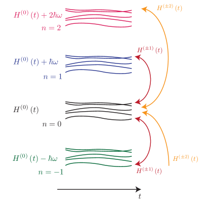
Figure 1: Schematic visualization of the terms which enter the slowly varying extended space Hamiltonian $\hat{K}=\hat{K}\left(t\right)$ given by Eqs. (11) and (12). Levels belonging to different Floquet bands $\left|\overline{n}\right\rangle$ are drawn in different colors. The operators $H^{\left(l\right)}(t)$ with $l\neq 0$ induce transitions between different Floquet bands. The operators $H^{\left(0\right)}(t)-n\hbar\omega$ provide the time-dependent zero-order eigenenergies of the extended-space Hamiltonian.

It is instructive that adding to $\hat{K}$ a unit operator $\hat{I}$ times $l\hbar\omega$ is equivalent to transforming $\hat{K}$ by a unitary operator $\hat{P}_{l}$

$$\hat{K}+l\hbar\omega\hat{I}=\hat{P}_{l}^{\dagger}\hat{K}\hat{P}_{l}$$ (13)

with

$$\hat{P}_{l}=\sum_{n=-\infty}^{\infty}\left|\overline{n+l}\right\rangle\left\langle\overline{n}\right|.$$ (14)

The operator $\hat{P}_{l}$ shifts an abstract state vector by $l$: $\left|\overline{n}\right\rangle\rightarrow\left|\overline{n+l}\right\rangle$. The relation (13) implies that the spectrum of $\hat{K}$ is invariant to shifting the energy by a multiple of $\hbar\omega$. In fact, the operators $\hat{K}$ and $\hat{P}_{l}^{\dagger}\hat{K}\hat{P}_{l}$ are related by a unitary transformation and hence commute and have the same set of eigenstates. This property will be used in the subsequent analysis of the high-frequency expansion of the Hamiltonian.

II.5 Initial condition and subsequent evolution

Let us consider a family of $\theta$-dependent state vectors $\left|\phi_{\theta}\left(t\right)\right\rangle$. At the initial time $t=t_{0}$ the state vector must be chosen periodic in $\theta$ according to Eq. (4). For convenience, we take a $\theta$-independent initial condition: $\left|\phi_{\theta}\left(t_{0}\right)\right\rangle=\left|\alpha\right\rangle$, where $\left|\alpha\right\rangle$ is an initial state vector. In that case, the transformed state vector $\left|\psi_{\theta}\left(t\right)\right\rangle$ is also $\theta$-independent at the initial time $t=t_{0}$:

$$\left|\psi_{\theta}\left(t_{0}\right)\right\rangle=\left|\phi_{\theta-\omega t_{0}}\left(t_{0}\right)\right\rangle=\left|\alpha\right\rangle\quad\textrm{for all }\theta\in\left[0,2\pi\right).$$ (15)

Therefore, initially one populates only the $n=0$ harmonic (in the phase variable $\theta$) in the Fourier expansion of the original or transformed state vector. In the abstract notation, the initial state vector contains only the mode $\left|\overline{n}\right\rangle$ with $n=0$ in Eqs. (10):

$$\left|\phi\left(t_{0}\right)\right\rrangle=\left|\psi\left(t_{0}\right)\right\rrangle=\left|\alpha\right\rangle\left|\overline{0}\right\rangle.$$ (16)

Subsequently, for $t>t_{0}$ the state vector $\left|\psi_{\theta}\left(t\right)\right\rangle$ becomes $\theta$ dependent due to the $\theta$ dependence of the Hamiltonian $\hat{K}\left(\theta,t\right)$ governing its temporal evolution in Eq. (8). This means the modes $\left|\overline{n}\right\rangle$ with $n\neq 0$ appear in the abstract state vector $\left|\psi\left(t\right)\right\rrangle$ during its subsequent time evolution described by the TDSE:

$$i\hbar\partial_{t}\left|\psi\left(t\right)\right\rrangle=\hat{K}(t)\left|\psi\left(t\right)\right\rrangle.$$ (17)

The dynamics governed by this equation will be analyzed in the next section.

III Temporal evolution and high frequency expansion

We shall make use of the symmetries of the Hamiltonian $\hat{K}(t)$ for its block diagonalization. In doing so, we shall include also the slow temporal dependence of $\hat{K}(t)$. We shall concentrate on a high-frequency limit where $\omega$ exceeds all other frequencies of the physical system. This will enable one to find a high-frequency expansion of an effective Hamiltonian $H_{\textrm{eff}}\left(t\right)$ taking into account the slow temporal dependence of $\hat{K}(t)$.

III.1 Block diagonalization

We shall look for a unitary transformation

$$\hat{D}^{\dagger}\left(t\right)\left|\psi\left(t\right)\right\rrangle=\left|\chi\left(t\right)\right\rrangle$$ (18)

which leads to a TDSE

$$i\hbar\partial_{t}\left|\chi\left(t\right)\right\rrangle=\hat{K}_{D}(t)\left|\chi\left(t\right)\right\rrangle$$ (19)

governed by a block-diagonal (in the extended space) Hamiltonian

$$\hat{K}_{D}\left(t\right)=\hat{D}^{\dagger}\left(t\right)\hat{K}\left(t\right)\hat{D}\left(t\right)-i\hbar\hat{D}^{\dagger}\left(t\right)\dot{\hat{D}}\left(t\right)$$ (20)

$$=\sum_{n}\left|\overline{n}\right\rangle\left(H_{\textrm{eff}}\left(t\right)+n\hbar\omega\right)\left\langle\overline{n}\right|\,.$$

Here $H_{\textrm{eff}}\left(t\right)$ entering the block-diagonal operator $\hat{K}_{D}\left(t\right)$ represents a slowly varying Floquet Hamiltonian describing an effective evolution of the physical system. It is instructive that the transformed Hamiltonian $\hat{K}_{D}\left(t\right)$ contains an additional term $i\hbar\hat{D}^{\dagger}\left(t\right)\dot{\hat{D}}\left(t\right)$ due to the temporal dependence of the unitary transformation $\hat{D}\left(t\right)$. Therefore, the block diagonalization is to be carried out in a self-consistent manner with respect to $\hat{D}\left(t\right)$.

Denoting

$$\hat{N}=\sum_{n=-\infty}^{\infty}\left|\overline{n}\right\rangle n\left\langle\overline{n}\right|\,\quad\mathrm{and}\quad\hat{I}=\sum_{n=-\infty}^{\infty}\left|\overline{n}\right\rangle\left\langle\overline{n}\right|\,,$$ (21)

one can write

$$\hat{K}_{D}\left(t\right)=\hbar\omega\hat{N}+H_{\textrm{eff}}\left(t\right)\hat{I}\,.$$ (22)

It is noteworthy that $H_{\textrm{eff}}\left(t\right)$ is not necessarily diagonal in the physical space. Furthermore, the block diagonalization is not a unique procedure. It is defined only up to a unitary transformation in the physical space, the same for each block comprising $\hat{K}_{D}$ in Eqs. (20)–(22). However, performing a high-frequency expansion in the powers of $1/\omega$, the block-diagonal operator $\hat{K}_{D}$ becomes unique provided the zero-order term of the diagonalization operator $\hat{D}$ is set to a unit operator, $\hat{D}_{\left(0\right)}=\hat{I}$. In fact, in the limit of an infinite frequency, $H^{\left(l\right)}/\omega\rightarrow 0$, the off-diagonal elements $H^{\left(l\right)}$ (with $l\neq 0$) of the extended-space Hamiltonian $\hat{K}$ can be neglected by replacing $\hat{K}\rightarrow\hbar\omega\hat{N}+H^{\left(0\right)}\hat{I}\,$. This means that for $H^{\left(l\right)}/\omega\rightarrow 0$ one can take: $\hat{D}=\hat{D}_{\left(0\right)}=\hat{I}$.

Note also that a block diagonalization similar to that in Eq. (20) has been employed in Ref. Eckardt and Anisimovas (2015) when dealing with a high-frequency expansion of the effective Hamiltonian $H_{\textrm{eff}}$ (see also Refs. Goldman and Dalibard (2014); Eckardt and Anisimovas (2015); Bukov et al. (2015); Mikami et al. (2016); Eckardt ). However, in the present situation the extended-space Hamiltonian $\hat{K}\left(t\right)$ additionally depends on a slow time, so the effective Hamiltonian $H_{\textrm{eff}}\left(t\right)$ and the diagonalization operator $\hat{D}$ are also time dependent. Furthermore, an extra term $i\hbar\hat{D}^{\dagger}\dot{\hat{D}}$ in Eq. (20) provides additional contributions to the high-frequency expansions of these operators due to the temporal changes of the components $H^{\left(l\right)}\left(t\right)$ entering the physical Hamiltonian (2), as we shall see in Sec. III.4.

In this way, our formalism combines two approaches: a systematic high-frequency expansion of $H_{\textrm{eff}}\left(t\right)$ via a degenerate perturbation theory in the extended Floquet space Eckardt and Anisimovas (2015), as well as an adiabatic perturbation theory Drese and Holthaus (1999); Weinberg et al. with respect to the basis vectors $\left|\overline{n}\right\rangle$ of the subspace $\mathscr{T}$ due to the temporal changes of the block-diagonalization operator $\hat{D}(t)$.

The relation (13) implies that the unitary operator $\hat{D}$ diagonalizing $\hat{K}$ is invariant with respect to the shift operator: $\hat{D}\left(t\right)=\hat{P}_{l}^{\dagger}\hat{D}\left(t\right)\hat{P}{}_{l}$. This is the case if $\hat{D}$ has the following form Eckardt and Anisimovas (2015):

$$\hat{D}\left(t\right)=\sum_{m,n=-\infty}^{\infty}D^{(m-n)}\left(t\right)\left|\overline{m}\right\rangle\left\langle\overline{n}\right|=\sum_{l=-\infty}^{\infty}D^{(l)}\left(t\right)\hat{P}_{l}\,.$$ (23)

III.2 Temporal evolution in the extended space

Since $\hat{K}_{D}\left(t\right)$ entering the TDSE (19) is block diagonal, the temporal evolution of the transformed state vector $\left|\chi\left(t\right)\right\rrangle=\sum_{n}\left|\chi_{n}\left(t\right)\right\rangle\left|\overline{n}\right\rangle$ is described by a set of uncoupled TDSEs for the constituting state vectors $\left|\chi_{n}\left(t\right)\right\rangle$ governed by the Hamiltonians $H_{\textrm{eff}}\left(t\right)+n\hbar\omega$. As a result, the time evolution of the transformed state vector $\left|\chi\left(t\right)\right\rrangle$ is given by

$$\left|\chi\left(t\right)\right\rrangle=\sum_{n=-\infty}^{\infty}\exp\left[-in\omega\left(t-t_{0}\right)\right]\left|\overline{n}\right\rangle U_{\textrm{eff}}\left(t,t_{0}\right)\left|\chi_{n}\left(t_{0}\right)\right\rangle\,,$$ (24)

where a unitary operator $U_{\textrm{eff}}\left(t,t_{0}\right)$ describes a quantum evolution in the physical space $\mathscr{H}$ generated by the effective Hamiltonian $H_{\textrm{eff}}\left(t\right)$:

$$i\hbar\partial_{t}U_{\textrm{eff}}\left(t,t_{0}\right)=H_{\textrm{eff}}\left(t\right)U_{\textrm{eff}}\left(t,t_{0}\right)\,,\quad U_{\textrm{eff}}\left(t_{0},t_{0}\right)=I.$$ (25)

If the effective Hamiltonian does not commute with itself at different times $\left[H_{\textrm{eff}}\left(t^{\prime}\right),H_{\textrm{eff}}\left(t^{\prime\prime}\right)\right]\neq 0$, a formal solution to this equation involves a time ordering

$$U_{\textrm{eff}}\left(t,t_{0}\right)={\cal T}\exp\left[-\frac{i}{\hbar}\int_{t_{0}}^{t}H_{\textrm{eff}}\left(t^{\prime}\right)\mathrm{d}t^{\prime}\right]\,.$$ (26)

For sufficiently slow changes of $H_{\textrm{eff}}\left(t^{\prime}\right)$ the adiabatic approximation Berry (1984); Mead (1992) can be applied to find the evolution operator $U_{\textrm{eff}}\left(t,t_{0}\right)$ on the basis of instantaneous eigenstates of $H_{\textrm{eff}}\left(t^{\prime}\right)$.

Combining Eqs. (16) and (18), the initial condition for the transformed state vector reads as $\left|\chi\left(t_{0}\right)\right\rrangle=\hat{D}^{\dagger}\left(t_{0}\right)\left|\overline{0}\right\rangle\left|\alpha\right\rangle$, giving

$$\left|\chi_{n}\left(t_{0}\right)\right\rangle=D^{\left(-n\right)\dagger}\left(t_{0}\right)\left|\alpha\right\rangle,$$ (27)

where $D^{(m-n)}=\left\langle\overline{m}\right|\hat{D}\left(t\right)\left|\overline{n}\right\rangle$ is an operator acting in the physical space $\mathscr{H}$. Substituting Eq. (27) into (24), the extended-space state vector $\left|\psi\left(t\right)\right\rrangle=\hat{D}\left(t\right)\left|\chi\left(t\right)\right\rrangle$ can be expressed in terms of the initial state vector $\left|\alpha\right\rangle$ and the matrix elements of the transformation operator $\hat{D}\left(t\right)$:

$$\left|\psi\left(t\right)\right\rrangle=\sum_{n,l=-\infty}^{\infty} \left|\overline{l}\right\rangle D^{\left(l-n\right)}\left(t\right)e^{-in\omega\left(t-t_{0}\right)}$$ (28)

$$\times U_{\textrm{eff}}\left(t,t_{0}\right)D^{\left(-n\right)\dagger}\left(t_{0}\right)\left|\alpha\right\rangle\,.$$

III.3 Temporal evolution in the physical space

Transition to the $\theta$ representation $\left|\psi\left(t\right)\right\rrangle\rightarrow\left|\psi_{\theta}\left(t\right)\right\rrangle$ is carried out replacing $\left|\overline{l}\right\rangle\rightarrow e^{il\theta}$ in Eq. (28). Using Eq. (7), one arrives at the extended-space state vector in the original representation $\left|\phi_{\theta}\left(t\right)\right\rrangle=\left|\psi_{\theta+\omega t}\left(t\right)\right\rrangle$. It can be treated as a state vector $\left|\phi_{\theta}\left(t\right)\right\rangle$ of the physical space $\mathscr{H}$ exhibiting a parametric dependence on the phase $\theta$ featured in the Hamiltonian $H\left(\theta+\omega t,t\right)$:

$$\left|\phi_{\theta}\left(t\right)\right\rangle$$ (29)

$$=U_{\textrm{Micro}}\left(\omega t+\theta,t\right)U_{\textrm{eff}}\left(t,t_{0}\right)U_{\textrm{Micro}}^{\dagger}\left(\omega t_{0}+\theta,t_{0}\right)\left|\alpha\right\rangle\,,$$

where

$$U_{\textrm{Micro}}\left(\omega t+\theta,t\right)=\sum_{n=-\infty}^{\infty}D^{\left(n\right)}\left(t\right)e^{in\left(\omega t+\theta\right)}\,.$$ (30)

is a unitary operator describing the micromotion (see Appendix A). It can be cast in the exponential form $U_{\textrm{Micro}}=\exp\left(-iS_{\textrm{Micro}}\right)$, where a Hermitian operator $S_{\textrm{Micro}}$ featured in the exponent is usually referred to as a micromotion operator (known also as a kick operator) Rahav et al. (2003); Eckardt and Anisimovas (2015); Goldman and Dalibard (2014); Bukov et al. (2015); Eckardt . We will use the term “micromotion operator” also for the unitary operator $U_{\textrm{Micro}}$.

Equation (29) represents a generalization of the Floquet theorem to periodically modulated Hamiltonians $H\left(\omega t+\theta,t\right)$ containing an extra temporal dependence. The dynamics of the system is then described in an effective manner by the slowly varying Hamiltonian $H_{\textrm{eff}}=H_{\textrm{eff}}\left(t\right)$ via the unitary operator $U_{\textrm{eff}}\left(t,t_{0}\right)$ defined by Eqs. (25) and (26). Additionally the solution (29) contains the micromotion operator $U_{\textrm{Micro}}\left(\omega t+\theta,t\right)$ calculated at the initial and final times $t=t_{0}$ and $t$.

It is instructive that the effective Hamiltonian $H_{\textrm{eff}}\left(t\right)$ and hence the unitary operator $U_{\textrm{eff}}\left(t,t_{0}\right)$ describing an effective long time evolution in Eq. (29) do not depend on the phase $\theta$ entering the original Hamiltonian $H\left(\theta+\omega t,t\right)$. Only the micromotion operators $U_{\textrm{Micro}}\left(\omega t+\theta,t\right)$ and $S_{\textrm{Micro}}\left(\omega t+\theta,t\right)$ are $\theta$ dependent. Yet, in comparison to the previous studies Eckardt and Anisimovas (2015); Goldman and Dalibard (2014); Bukov et al. (2015); Eckardt , the operator $U_{\textrm{Micro}}\left(\omega t+\theta,t\right)$ includes not only the fast micromotion represented by the exponential factors $e^{in\left(\omega t+\theta\right)}$ in Eq. (30), but also an additional temporal dependence due to slow changes of the transformation $\hat{D}\left(t\right)$ diagonalizing the extended-space Floquet Hamiltonian $\hat{K}\left(t\right)$ in Eq. (20). In particular, this is the case if the periodic perturbation is switched on and off in a smooth manner, which is relevant to, e.g., shaken optical lattices with a time-dependent shaking strength Eckardt et al. (2010); Aidelsburger et al. (2011); Arimondo et al. (2012); Hauke et al. (2012); Windpassinger and Sengstock (2013); Struck et al. (2013); Aidelsburger et al. (2013); Jotzu et al. (2014); Aidelsburger et al. (2015); Kennedy et al. (2015); Fläschner et al. (2016). In that case, the micromotion operator featured in Eq. (29) reduces to the unit operator

$$\left.U_{\textrm{Micro}}^{\dagger}\left(\omega t+\theta,t\right)\right|_{t=t_{0}}=1$$ (31)

at the initial time $t_{0}$, when the periodic perturbation starts slowly switching on. In that case, the extended-space Hamiltonian $\hat{K}(t)$ given by Eq. (12) is block diagonal at the initial time $t=t_{0}$ when the periodic perturbation is off, so no subsequent block diagonalization is needed.

III.4 High-frequency expansion

Knowing the effective Hamiltonian $H_{\textrm{eff}}\left(t\right)$ and the micromotion operator $U_{\textrm{Micro}}\left(\omega t+\theta,t\right)$ one can use Eqs. (29) and (25) and (26) to find the time evolution of the state vector $\left|\phi_{\theta}\left(t\right)\right\rangle$ which parametrically depends on the phase $\theta$. Usually, both operators $H_{\textrm{eff}}\left(t\right)$ and $U_{\textrm{Micro}}\left(\omega t+\theta,t\right)$ can not be determined analytically. However, for sufficiently high driving frequencies, they can be expressed as a series expansion in the terms of the powers of $\omega^{-1}$. This can be done if off-diagonal matrix elements of the extended-space Hamiltonian (12) are small compared to the driving frequency, $\left|H_{\alpha\beta}^{\left(l\right)}\right|\ll\hbar\omega$, and the spectral width of the physical system is much smaller than driving frequency, $\left|\varepsilon_{\alpha}-\varepsilon_{\beta}\right|=\left|H_{\alpha\alpha}^{\left(0\right)}-H_{\beta\beta}^{\left(0\right)}\right|\ll\hbar\omega$. Furthermore, the operators $H^{\left(l\right)}$ should change little over a period of oscillations: $\left|\dot{H}_{\alpha\beta}^{\left(l\right)}\right|\ll\omega\left|H_{\alpha\beta}^{\left(l\right)}\right|$. The latter condition appears because the matrix elements of the operator $i\hbar\hat{D}^{\dagger}\left(t\right)\dot{\hat{D}}\left(t\right)$ featured in Eq. (20) should be much smaller than $\omega$.

In some cases, such as in shaken optical lattices Eckardt et al. (2010); Aidelsburger et al. (2011); Arimondo et al. (2012); Hauke et al. (2012); Windpassinger and Sengstock (2013); Struck et al. (2013); Aidelsburger et al. (2013); Jotzu et al. (2014); Aidelsburger et al. (2015); Kennedy et al. (2015); Fläschner et al. (2016), the spectrum of the physical system extends beyond the driving frequency, so the condition $\left|\varepsilon_{\alpha}-\varepsilon_{\beta}\right|\ll\hbar\omega$ does not hold for the states with high energies $\varepsilon_{\alpha}$. Yet, if these states are not directly accessible from the initial state of the system, the high-frequency expansion can still be used to describe the dynamics of the system at the intermediate times when the higher states are not yet populated Eckardt . In particular, it was demonstrated Kuwahara et al. (2016) that for time-periodic systems the truncated high-frequency expansion can remain applicable even when the condition $\left|\varepsilon_{\alpha}-\varepsilon_{\beta}\right|\ll\hbar\omega$ is not met. On the other hand, in many-body systems the adiabatic approximation may break down not only at very high ramp rates, but also at very slow ones due to avoided crossings of Floquet many-body resonances Eckardt and Holthaus (2008); Weinberg et al. ; Eckardt [Thiskindofbreakdowncanoccurnotonlyinmany-bodysystems; butalsoforsingle-particlesystems; suchasadrivenanharmonicoscillatororaparticleinasquarepotentialconsideredby][.Thesesystemsdonotpossesanadiabaticlimitintheusualsenseduetothedensenessofthequasienergyspectrum.]Hone97. This effect is not captured by the high-frequency expansion, but it should become smaller and smaller with increasing the ramp rates and driving frequency.

A general formalism of the high-frequency expansion is presented in Appendix B. Here, we summarize the findings. The effective Hamiltonian expanded in the powers of $\omega^{-1}$ reads as

$$H_{\textrm{eff}}=H_{\textrm{eff}\left(0\right)}+H_{\textrm{eff}\left(1\right)}+H_{\textrm{eff}\left(2\right)}+\ldots,$$ (32)

where the $n$th term $H_{\textrm{eff}\left(n\right)}$ is proportional to $\omega^{-n}$. The first three expansion terms are

$$H_{\textrm{eff}\left(0\right)} =H^{\left(0\right)},$$ (33a)

$$H_{\textrm{eff}\left(1\right)} =\frac{1}{\hbar\omega}\sum_{m=1}^{\infty}\frac{1}{m}\left[H^{\left(m\right)},H^{\left(-m\right)}\right],$$ (33b)

$$H_{\textrm{eff}\left(2\right)} =\frac{1}{\left(\hbar\omega\right)^{2}}\sum_{m\neq 0}\left\{\frac{\left[H^{\left(-m\right)},\left[H^{\left(0\right)},H^{\left(m\right)}\right]\right]-i\hbar\left[H^{\left(-m\right)},\dot{H}^{\left(m\right)}\right]}{2m^{2}}+\sum_{n\neq\left\{0,m\right\}}\frac{\left[H^{\left(-m\right)},\left[H^{\left(m-n\right)},H^{\left(n\right)}\right]\right]}{3mn}\right\},$$ (33c)

where the (slow) temporal dependence of the components $H^{\left(n\right)}=H^{\left(n\right)}\left(t\right)$ is kept implicit.

Note that the second-order contribution proportional to $\left[H^{\left(-m\right)},\dot{H}^{\left(m\right)}\right]$ stems from projecting onto a selected Floquet band (with $n=0$) of an extra term $-i\hbar\hat{D}^{\dagger}\left(t\right)\dot{\hat{D}}\left(t\right)$ entering Eq. (20). This provides a geometric phase Berry (1984) for an adiabatic motion in the selected Floquet band. The geometric phase can be non-Abelian if more than one quantum state is involved in the adiabatic motion Wilczek and Zee (1984); Moody et al. (1986); Zee (1988). In Sec. IV we shall consider an example providing non-Abelian geometric phases for the adiabatic motion in the Floquet band.

Expanding the Hermitian micromotion operator $S_{\textrm{Micro}}$ entering $U_{\textrm{Micro}}=\exp\left(-iS_{\textrm{Micro}}\right)$ in the series $S_{\textrm{Micro}}=S_{\textrm{Micro}\left(1\right)}+S_{\textrm{Micro}\left(2\right)}+\ldots$, the first- and the second-order terms read as

$$S_{\textrm{Micro}\left(1\right)}\left(\theta^{\prime},t\right)=\frac{1}{i\hbar\omega}\sum_{m\neq 0}\frac{1}{m}H^{\left(m\right)}e^{im\theta^{\prime}},$$ (34a)

$$S_{\textrm{Micro}\left(2\right)}\left(\theta^{\prime},t\right)=\frac{1}{2i\left(\hbar\omega\right)^{2}}\sum_{m\neq 0}\left\{\frac{1}{m^{2}}\left[H^{\left(m\right)},H^{\left(0\right)}\right]+\sum_{n\neq 0}\frac{1}{mn}\left[H^{\left(n\right)},H^{\left(m-n\right)}\right]+\frac{2i\hbar}{m^{2}}\dot{H}^{\left(m\right)}\right\}e^{im\theta^{\prime}},$$ (34b)

where $\theta^{\prime}=\omega t+\theta$.

On the other hand, the expansion of the operator $U_{\textrm{Micro}}\left(\theta^{\prime},t\right)$ up to the $\omega^{-3}$ order is given by

$$U_{\textrm{Micro}}\left(\theta^{\prime},t\right) =\mathbf{1}_{\mathscr{H}}-\frac{1}{\hbar\omega}\sum_{m\neq 0}\frac{1}{m}H^{\left(m\right)}e^{im\theta^{\prime}}+\frac{1}{2\left(\hbar\omega\right)^{2}}\sum_{m\neq 0}\sum_{n\neq 0}e^{i\left(m+n\right)\theta^{\prime}}\frac{H^{\left(m\right)}H^{\left(n\right)}}{nm}$$

$$+\frac{1}{2\left(\hbar\omega\right)^{2}}\sum_{m\neq 0}e^{im\theta^{\prime}}\left\{\frac{\left[H^{\left(0\right)},H^{\left(m\right)}\right]-2i\hbar\dot{H}^{\left(m\right)}}{m^{2}}-\sum_{n\neq 0}\frac{\left[H^{\left(n\right)},H^{\left(m-n\right)}\right]}{nm}\right\}+\mathcal{O}\left(\omega^{-3}\right)\,.$$ (35)

Although the operator $U_{\textrm{Micro}}$ is unitary, it becomes non-unitary if approximated with a finite number of terms. For instance, in Eq. (35) the unitarity holds up to the $\omega^{-3}$ order.

Generalizing Refs. Eckardt and Anisimovas (2015); Goldman and Dalibard (2014); Bukov et al. (2015); Mikami et al. (2016); Eckardt , the expanded effective Hamiltonian and micromotion operators are now time dependent due to the temporal dependence of the components $H^{\left(m\right)}=H^{\left(m\right)}\left(t\right)$ entering the expansions. For instance, if the amplitude of the periodic perturbation applied to the system slowly increases from zero reaching a saturation value at $t$, the operator $U_{\textrm{Micro}}(t)$ is the unit operator at $t=t_{0}$, and reaches a stationary oscillating solution at the saturation times $t$. Furthermore, in the present situation the effective Hamiltonian and micromotion operators acquire additional terms due to the slow temporal dependence of the harmonics $H^{\left(m\right)}\left(t\right)$. Specifically, the term proportional to $\left[H^{\left(-m\right)},\dot{H}^{\left(m\right)}\right]$ appears as the second-order correction to the effective Hamiltonian in Eq. (33c). On the other hand, the terms proportional to $\dot{H}^{\left(m\right)}$ represent the first-order correction to the micromotion operators in Eqs. (34b) and (35).

The high-frequency expansion of the Hamiltonian is often restricted to the zero and first orders, in which the extra term $\propto\left[H^{\left(-m\right)},\dot{H}^{\left(m\right)}\right]$ does not show up. In that case one can simply replace the time-independent effective Hamiltonian obtained for the stationary driving by the time dependent one. For example, shaking of optical lattices is known to renormalize inter-site tunneling amplitudes Eckardt et al. (2005); Lignier et al. (2007); Arimondo et al. (2012); Bukov et al. (2015); Eckardt which acquire a slow temporal dependence in the case of a slowly varying driving. In Appendix C, this is illustrated for a one-dimensional shaken optical lattice with a slowly changing amplitude of driving.

In the following Sec. IV we will consider a spin in an oscillating magnetic field with a changing direction. In that case, there are no zero- and first-order contributions to the effective Hamiltonian. Therefore, the second-order term proportional to $\left[H^{\left(-m\right)},\dot{H}^{\left(m\right)}\right]$ represents a dominant contribution which plays a vital role in the system dynamics providing non-Abelian geometric phases.

IV Spin in an oscillating magnetic field

Let us apply the general formalism to a spin in a fast oscillating magnetic field $\mathbf{B}\left(t\right)\cos\left(\omega t+\theta\right)$ with a slowly varying amplitude $\mathbf{B}\left(t\right)$. Such a system is described by a Hamiltonian

$$H\left(\omega t+\theta,t\right)=g_{F}\mathbf{F}\cdot\mathbf{B}\left(t\right)\cos\left(\omega t+\theta\right)\,,$$ (36)

where $g_{F}$ is a gyromagnetic factor, $\mathbf{F}=F_{1}\mathbf{e}_{x}+F_{2}\mathbf{e}_{y}+F_{3}\mathbf{e}_{z}$ is a spin operator satisfying the usual commutation relations $\left[F_{l},F_{m}\right]=i\hbar\epsilon_{lmn}F_{n}$. Here, $\epsilon_{lmn}$ is a Levi-Civita symbol, and a summation over a repeated Cartesian index $n=1,2,3$ is implied. The non-zero Fourier components of the Hamiltonian (36) are

$$H^{\left(1\right)}=H^{\left(-1\right)}=\frac{g_{F}}{2}\mathbf{F}\cdot\mathbf{B}\left(t\right).$$ (37)

We now obtain the effective Hamiltonian and the micromotion operators up to the second order in $\omega^{-1}$ inclusively. Calling on Eqs. (32) and (33), the truncated effective Hamiltonian reads as:

$$H_{\textrm{eff}} =H_{\textrm{eff}\left(2\right)}=\frac{-i\hbar}{\left(\hbar\omega\right)^{2}}\left[H^{\left(1\right)},\dot{H}^{\left(1\right)}\right]$$ (38)

$$=\frac{-i\hbar g_{F}^{2}}{\left(2\hbar\omega\right)^{2}}B_{k}\dot{B}_{l}\left[F_{k},F_{l}\right]$$

$$=g_{F}^{2}\left(2\omega\right)^{-2}\epsilon_{klm}B_{k}\dot{B}_{l}F_{m}$$

$$=g_{F}^{2}\left(2\omega\right)^{-2}\mathbf{F}\cdot\left(\mathbf{B}\times\dot{\mathbf{B}}\right).$$

Using Eq. (34a), the first-order micromotion operator is given by:

$$S_{\textrm{Micro}(1)}\left(\omega t+\theta,t\right)=\frac{g_{F}}{\hbar\omega}\mathbf{F}\cdot\mathbf{B}\left(t\right)\sin\left(\omega t+\theta\right)\,.$$ (39)

The second-order contribution to the micromotion given by (34b) appears now due to ramping of the magnetic field:

$$S_{\textrm{Micro}\left(2\right)}\left(\omega t+\theta,t\right)=\frac{g_{F}}{\hbar\omega^{2}}\mathbf{F}\cdot\dot{\mathbf{B}}\left(t\right)\cos\left(\omega t+\theta\right).$$ (40)

According to Eq. (38), the change in the orientation of the magnetic field provides an effective Hamiltonian $H_{\textrm{eff}}$ proportional to the spin perpendicular to both the magnetic field $\mathbf{B}$ and its derivative $\dot{\mathbf{B}}$, i.e., perpendicular to the rotation plane for the magnetic field. If the plane of the rotation is changing, the Hamiltonian does not commute with itself at different times, so the time ordering is needed in the evolution operator $U_{\textrm{eff}}\left(t,t_{0}\right)$ presented in Eq. (42) below. The effective evolution of the spin is then associated with non-Abelian (noncommuting) geometric phases, as we shall see below.

It is to be emphasized that in the present situation the geometric phases appear because the effective evolution of the physical system involves the adiabatic elimination of the Floquet bands with $m\neq 0$ in the extended space, as generally illustrated in Fig. 1. Thus, the emerging non-Abelian phases reflect the geometry of the extended Floquet space rather than that of the physical one.

To see the geometric nature of the effective Hamiltonian (38), it is convenient to represent it in terms of a geometric vector potential $\mathbf{{\cal A}}$:

$$H_{\textrm{eff}}=\mathbf{{\cal A}}\cdot\dot{\mathbf{B}}\,,\qquad\mathbf{{\cal A}}=g_{F}^{2}\left(2\omega\right)^{-2}\left(\mathbf{F}\times\mathbf{B}\right)\,.$$ (41)

The evolution operator (26) then takes the form

$$U_{\textrm{eff}}\left(t,t_{0}\right)={\cal T}\exp\left[-\frac{i}{\hbar}\int_{t_{0}}^{t}\mathbf{{\cal A}}\cdot d\mathbf{B}\left(t^{\prime}\right)\right]\,.$$ (42)

The operator $U_{\textrm{eff}}\left(t,t_{0}\right)$ is thus determined by a path of the magnetic field, not by a speed of its change, showing a geometric origin of the acquired phases.

In particular, performing an anticlockwise rotation of the magnetic field $\mathbf{B}$ by an angle $\varphi$ in a plane orthogonal to a unit vector $\mathbf{n}\propto\mathbf{B}\times\dot{\mathbf{B}}$, the corresponding evolution operator is defined by a spin along the rotation direction: $\mathbf{F}\cdot\mathbf{n}$. If additionally an amplitude $B$ of the rotating magnetic field is not changing, the evolution operator (42) simplifies to

$$U_{\textrm{eff}}\left(\mathbf{n},\varphi\right)=\exp\left[-\frac{i}{\hbar}\gamma_{\varphi}\mathbf{F}\cdot\mathbf{n}\right]\,,\qquad\gamma_{\varphi}=\varphi\frac{g_{F}^{2}B^{2}}{4\omega^{2}}\,.$$ (43)

After making $l$ rotations, the angle is given by $\varphi=2\pi l$, where $l$ is an integer. In that case, the magnetic field $\mathbf{B}\left(t\right)$ comes back to its original value. Therefore, the exponent $\gamma_{\varphi}\mathbf{F}\cdot\mathbf{n}/\hbar$ can be identified as a Wilczek-Zee phase operator Wilczek and Zee (1984) representing a non-Abelian generalization to the Berry phase Berry (1984). The corresponding eigenvalues $\gamma_{\varphi}m_{F}$ linearly depend on the spin projection $m_{F}$ along the rotation axis $\mathbf{n}$. For a single loop ($l=1$) the phase $\gamma_{\varphi}$ is much smaller than the unity because of the assumption of the high-frequency driving. Performing many loops ($l\gg 1$), one may accumulate a considerable phase $\gamma_{\varphi}$. It is noteworthy that two consecutive rotations along non-parallel axes $\mathbf{n}^{\prime}$ and $\mathbf{n}^{\prime\prime}$ do not commute $\left[U_{\textrm{eff}}\left(\mathbf{n}^{\prime},\varphi^{\prime}\right),U_{\textrm{eff}}\left(\mathbf{n}^{\prime\prime},\varphi^{\prime\prime}\right)\right]\neq 0$. This demonstrates a non-Abelian character of the problem.

As shown in Appendix D, the acquired geometric phase $\gamma_{\varphi}\mathbf{F}\cdot\mathbf{n}/\hbar$ entering the evolution operator (43) stems from the rotational frequency shift Bialynicki-Birula and Bialynicka-Birula (1997) representing a correction to it. The correction term to the effective Hamiltonian presented by Eq. (93c) is proportional to the spin along the rotation direction, in agreement with Eqs. (38) and (43).

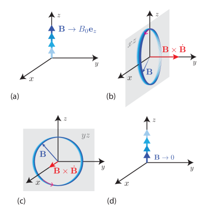
Figure 2: An example of a spin driven by an oscillating magnetic field. The scheme involves four stages which include raising of the magnetic field along the $z$ axis (a), subsequent rotation of the magnetic field along the $y$ and $x$ axes (b), (c), and switching off the magnetic field which again points along the $z$ axis (d).

The effect of the geometric phases can be measured using, for instance, the following sequence illustrated in Fig. 2. Initially at $t=t_{0}$ the oscillating magnetic field and its derivative are zero: $B\left(t_{0}\right)\rightarrow 0$ and $\dot{B}\left(t_{0}\right)\rightarrow 0$. Therefore, according to the Eq. (31), the micromotion is absent at the initial time: $U_{\textrm{Micro}}\left(\omega t_{0}+\theta,t_{0}\right)=1$. Subsequently, for $t_{0}<t<t_{1}$ the magnetic field strength increases until reaching a steady-state value $B=B_{0}$. In doing so, the direction of the magnetic field is kept fixed along the $z$ axis ($\mathbf{B}\left(t\right)\parallel\mathbf{e}_{z}$), as indicated in Fig. 2 (a). The effective Hamiltonian $H_{\textrm{eff}}$ is then zero. Therefore, apart from the micromotion there is no other dynamics at this stage: $U_{\textrm{eff}}\left(t_{1},t_{0}\right)=1$. In the next interval $t_{1}<t<t_{2}$ the magnetic field maintains a constant amplitude $B_{0}$ and changes its direction, so non-zero effective Hamiltonian $H_{\textrm{eff}}$ contributes to the temporal evolution of the system. During that stage, the magnetic field may perform a number rotations along different axes $\mathbf{n}_{j}$, described by non-commuting unitary operators $U_{\textrm{eff}}\left(\mathbf{n}_{j},\varphi_{j}\right)$. This is illustrated in Figs 2 (b) and (c) showing two rotations: along the $y$ and $x$ axes ($\mathbf{n}_{j}=\mathbf{e}_{y},\,\mathbf{e}_{x}$). In the final interval $t_{2}<t<t_{3}$, the magnetic field is decreasing without changing its direction, so that $H_{\textrm{eff}}=0$ and hence $U_{\textrm{eff}}\left(t_{3},t_{2}\right)=1$. At the final time $t=t_{3}$, the magnetic field and its derivative go to zero $B\left(t_{3}\right)\rightarrow 0$ and $\dot{B}\left(t_{3}\right)\rightarrow 0$ (see Fig. 2 (d)), so the micromotion vanishes.

Since there is no micromotion at the initial and final times: $U_{\textrm{Micro}}\left(\omega t_{0}+\theta,t_{0}\right)=U_{\textrm{Micro}}\left(\omega t_{3}+\theta,t_{3}\right)=1$, according to Eq. (29) the state vector at the final time is related to that at the initial time by a $\theta$-independent effective evolution operator $U_{\textrm{eff}}\left(t_{3},t_{0}\right)=U_{\textrm{eff}}\left(t_{2},t_{1}\right)$:

$$\left|\phi_{\theta}\left(t_{3}\right)\right\rangle=U_{\textrm{eff}}\left(t_{3},t_{0}\right)\left|\alpha\right\rangle=U_{\textrm{eff}}\left(t_{2},t_{1}\right)\left|\alpha\right\rangle$$ (44)

In this way, the long-time dynamics of state vector is described by the same effective evolution operator $U_{\textrm{eff}}\left(t_{3},t_{0}\right)$ for an arbitrary phase $\theta$ entering the Hamiltonian $H\left(\omega t+\theta,t\right)$. This makes the scheme insensitive to the phase $\theta$ and a way the magnetic field is switched on and off.

It is noteworthy that the dynamics of a spin adiabatically following a slowly changing magnetic field was considered by Berry Berry (1984). In that case, an adiabatic elimination of the second spin component provided a geometric (Berry) phase after a cyclic evolution. Such a geometric phase is Abelian, because the effective dynamics involves a single-spin component adiabatically following the magnetic field.

In the present situation relying on a fast oscillating magnetic field with a changing direction, the spin is no longer adiabatically following the magnetic field. Therefore, the spin degree of freedom is no longer frozen and the emergence of the non-Abelian phases is possible. The non-Abelian geometric phases arise now due to adiabatic elimination of the extended space Floquet bands with $m\neq 0$ (shown in Fig. 1 and in Fig. 4(a) in Appendix D), rather than of the physical states, as it is usually the case Wilczek and Zee (1984); Moody et al. (1986); Zee (1988).

Finally, let us compare the analytical expression (43) for the effective dynamics with numerical simulations. For this we numerically calculate the exact evolution of a spin-$1/2$ particle governed by the Hamiltonian (36), in which the amplitude of the oscillating magnetic field $\mathbf{B}(t)=B\left[\mathbf{e}_{z}\cos(\Omega t)-\mathbf{e}_{y}\sin(\Omega t)\right]$ rotates in the $yz$ plane. After preparing the system in a spin-up state, $\left|\alpha\right\rangle=\left|\uparrow\right\rangle$, we allow the magnetic field vector $\mathbf{B}(t)$ to make $l=10$ rotations in the $yz$ plane. This transforms the state vector to a superposition of the spin-up and -down states: $c_{\uparrow}(t_{l})\left|\uparrow\right\rangle+c_{\downarrow}(t_{l})\left|\downarrow\right\rangle$, with $t_{l}=2\pi l/\Omega$. The corresponding probabilities $|c_{\uparrow}(2\pi l/\Omega)|^{2}$ and $|c_{\downarrow}(2\pi l/\Omega)|^{2}$ calculated numerically for $l=10$ are depicted by asterisks and circles in Fig. 3. To remove the fast oscillations due to the micromotion operators, the numerical simulations have been performed by taking the values of the driving frequency $\omega$ such that $l\omega/\Omega$ remains integer.

On the other hand, the effective evolution described by Eq. (43) yields the following analytical expressions for these probabilities:

$$|c_{\uparrow}(2\pi l/\Omega)|^{2} =\cos^{2}\left(\frac{\pi lg_{F}^{2}B^{2}}{4\omega^{2}}\right),$$ (45a)

$$|c_{\downarrow}(2\pi l/\Omega)|^{2} =\sin^{2}\left(\frac{\pi lg_{F}^{2}B^{2}}{4\omega^{2}}\right).$$ (45b)

As one can see from Fig. 3, the numerical results agree well with the analytical ones (shown in solid lines) when the driving frequency $\omega$ exceeds considerably the frequency of the magnetic field rotation: $\omega\gg\Omega$.

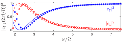
Figure 3: The probabilities $|c_{\uparrow}(2\pi l/\Omega)|^{2}$ and $|c_{\downarrow}(2\pi l/\Omega)|^{2}$ to find the spin in the states $\left|\uparrow\right\rangle$ (blue asterisk and solid line) and $\left|\downarrow\right\rangle$ (red circles and dashed line) after $l=10$ rotations of the magnetic field. The probabilities have been calculated numerically (symbols) and from the effective evolution Eqs. (45) (continuous lines). The characteristic amplitude of the magnetic field is taken to be such that $g_{F}B/\Omega=1$.

V Concluding remarks

We have considered a quantum system described by the Hamiltonian $H\left(\omega t+\theta,t\right)$ which is $2\pi$-periodic with respect to the first argument $\omega t+\theta$ and allows for an additional (slow) temporal dependence represented by the second argument. The periodic time-dependence of the Hamiltonian has been eliminated applying the extended-space formulation of the Floquet theory Guérin and Jauslin (2003). Consequently the original Schrödinger-type equation (3) has been transformed into an equivalent Schrödinger-like equation of motion (17) governed by the extended-space Hamiltonian (11) containing only a slow temporal dependence.

Using such an approach, Eq. (29) has been obtained describing the evolution of the system in terms of a long term dynamics governed by the $\theta$-independent unitary operator $U_{\textrm{eff}}\left(t,t_{0}\right)$, as well as the $\theta$-dependent micromotion operators $U_{\textrm{Micro}}\left(\omega t+\theta,t\right)$ taken at the initial and final times, $t=t_{0}$ and $t$. The former operator $U_{\textrm{eff}}\left(t,t_{0}\right)$ is determined by the effective Hamiltonian $H_{\textrm{eff}}=H_{\textrm{eff}}\left(t\right)$ slowly changing in time. The latter $U_{\textrm{Micro}}\left(\omega t+\theta,t\right)$ not only describes the fast periodic motion, but also exhibits an additional slow temporal dependence.

We have provided a general framework for a combined analysis of a high-frequency perturbation and slow changes in the periodic driving. The micromotion operators and the effective Hamiltonian have been systematically constructed in terms of a series in the powers of $\omega^{-1}$. Analytical expressions (32), (33), and (35) give the expansions to the second order in $\omega^{-1}$ inclusively.

In the limit of a strictly time-periodic Hamiltonian $H=H\left(\omega t+\theta\right)$, the expansions reproduce the ones presented in previous studies Eckardt and Anisimovas (2015); Goldman and Dalibard (2014); Bukov et al. (2015); Mikami et al. (2016); Eckardt . Yet, in a more general situation considered here, the effective Hamiltonian and the micromotion operators incorporate the dependence on the slow time. Thus, they change their form during the course of the evolution. Furthermore, the effective Hamiltonian and micromotion operators contain additional second-order contributions emerging entirely from the slow temporal dependence of the Fourier components composing the original Hamiltonian in Eq. (2).

To show the effect of the additional terms on the dynamics, in Sec. IV we have studied a spin $\hat{\mathbf{F}}$ in a magnetic field oscillating rapidly along a slowly changing direction. If the changes in the orientation of the magnetic field are not restricted to a single plane, the effective evolution of the spin provides non-Abelian geometric phases.

The general theory is applicable to other driven systems, such as periodically modulated optical lattices with a time-dependent forcing strength. Such a situation is relevant to cold-atom experiments Eckardt et al. (2010); Aidelsburger et al. (2011); Arimondo et al. (2012); Hauke et al. (2012); Windpassinger and Sengstock (2013); Struck et al. (2013); Aidelsburger et al. (2013); Jotzu et al. (2014); Aidelsburger et al. (2015); Kennedy et al. (2015); Fläschner et al. (2016). Shaking of optical lattices is known to renormalize inter-site tunneling amplitudes Eckardt et al. (2005); Lignier et al. (2007); Arimondo et al. (2012); Bukov et al. (2015); Eckardt . In the case of a slowly varying driving, the tunneling amplitudes acquire a slow temporal dependence. In Appendix C this is illustrated for a one-dimensional optical lattice affected by a slowly changing shaking.

If the periodic modulation is absent at the initial time $t_{0}$ and is slowly switched on afterwards, the micromotion operator $U_{\textrm{Micro}}^{\dagger}\left(\omega t_{0}+\theta,t_{0}\right)$ reduces to a unit operator in Eq. (29). In that case, the temporal evolution of the system is described by the effective Hamiltonian $H_{\textrm{eff}}=H_{\textrm{eff}}\left(t\right)$ slowly changing in time, and fast oscillating micromotion operator $U_{\textrm{Micro}}\left(\omega t+\theta,t\right)$ calculated only at the final time.

Appendix A Unitarity of the operator $U_{\textrm{Micro}}\left(\omega t+\theta,t\right)$

Here, we will show that the micromotion operator $U_{\textrm{Micro}}\left(\omega t+\theta,t\right)$ is unitary in the physical space. By definition, the operator $\hat{D}\left(t\right)$ is unitary in the extended space:

$$\hat{D}^{\dagger}\hat{D}=\sum_{n}\left|\overline{n}\right\rangle\mathbf{1}_{\mathscr{H}}\left\langle\overline{n}\right|\,,$$

where $\mathbf{1}_{\mathscr{H}}$ is a unit operator in the physical Hilbert space $\mathscr{H}$. On the other hand, using (23) for $\hat{D}\left(t\right)$ and the fact that $\hat{P}_{l}\hat{P}_{m}=\hat{P}_{m+l}$, one finds

$$\hat{D}^{\dagger}\hat{D}=\sum_{m,n}D^{\left(m\right)\dagger}D^{\left(n\right)}\hat{P}_{-m}\hat{P}_{n}=\sum_{m,l}D^{\left(m\right)\dagger}D^{\left(l+m\right)}\hat{P}_{l}\,.$$

Comparing the two equations, one obtains the following condition for $D^{\left(m\right)}$:

$$\sum_{m=-\infty}^{\infty}D^{\left(m\right)\dagger}D^{\left(m+l\right)}=\mathbf{1}_{\mathscr{H}}\delta_{l0}.$$ (46)

Consequently, one finds that the micromotion operator given by Eq. (30) is indeed unitary:

$$U_{\textrm{Micro}}^{\dagger}U_{\textrm{Micro}}=\sum_{m,n}D^{(m)\dagger}\left(t\right)D^{(n)}\left(t\right)e^{i\left(n-m\right)\omega t}=\mathbf{1}_{\mathscr{H}}\,.$$ (47)

Appendix B Expansion of the effective Hamiltonian in the powers of $1/\omega$

B.1 Basic initial equations

It is convenient to represent the abstract extended-space Hamiltonian (11) as

$$\hat{K}=\hbar\omega\hat{N}+\hat{K}^{\prime}\,,\quad\mathrm{with}\quad\hat{K}^{\prime}=\sum_{m=-\infty}^{+\infty}H^{\left(m\right)}\hat{P}_{m}\,,\,,$$ (48)

where $\hat{N}$ is the “number” operator in the Floquet basis given by Eq. (21), and $\hat{P}_{m}$ is defined by (14). Below we will use some properties of the operators $\hat{P}_{m}$, namely,

$$\left[\hat{P}_{m},\hat{N}\right]=-m\hat{P}_{m},\quad\hat{P}_{m}\hat{P}_{n}=\hat{P}_{m+n}\quad\textrm{and}\quad\left[\hat{P}_{m},\hat{P}_{n}\right]=0.$$ (49)

We are looking for a unitary transformation

$$\hat{D}\left(t\right)=e^{-i\hat{S}\left(t\right)}$$ (50)

which makes the Hamiltonian $\hat{K}$ given Eq. (48) diagonal in the abstract extended space:

$$\hat{D}^{\dagger}\hat{K}\hat{D}-i\hbar\hat{D}^{\dagger}\dot{\hat{D}}=e^{i\hat{S}}\hat{K}e^{-i\hat{S}}-i\hbar e^{i\hat{S}}\frac{d}{dt}e^{-i\hat{S}}=\hat{K}_{D}\,,$$ (51)

where

$$\hat{K}_{D}\left(t\right)=\hbar\omega\hat{N}+H_{\textrm{eff}}\left(t\right)\hat{P}_{0}\,.$$ (52)

is block diagonal.

B.2 High-frequency expansion

We are interested in a situation where the spectrum of $H_{\textrm{eff}}$ is confined in an energy range much smaller than the separation between the Floquet bands $\hbar\omega$. In that case, the effective Hamiltonian $H_{\textrm{eff}}$ can be expanded in powers of the inverse driving frequency $1/\omega$:

$$H_{\textrm{eff}}=H_{\textrm{eff}\left(0\right)}+H_{\textrm{eff}\left(1\right)}+H_{\textrm{eff}\left(2\right)}+\ldots\,.$$ (53)

where the $j$-th term $H_{\textrm{eff}\left(j\right)}$ is of the order of $1/\omega^{j}$. As we shall see later on, the zero-order term $H_{\textrm{eff}\left(0\right)}$ coincides with the contribution due to the zero-frequency component $H^{\left(0\right)}$ of the physical Hamiltonian.

The Hermitian operator $\hat{S}$ featured in the unitary transformation $\hat{D}$, Eq. (50), can also be expanded in the powers of $1/\omega$ as:

$$\hat{S}=\hat{S}_{\left(1\right)}+\hat{S}_{\left(2\right)}+\ldots\,,$$ (54)

where the expansion does not contain the zero-order term, because the unitary operator $\hat{D}=\exp\left(-i\hat{S}\right)$ should approach the unity in a very high-frequency limit.

We are also looking for the $1/\omega$ power expansion of the unitary operator $\hat{D}$:

$$\hat{D}=\hat{D}_{\left(0\right)}+\hat{D}_{\left(1\right)}+\hat{D}_{\left(2\right)}+\ldots\,,$$ (55)

with

$$\hat{D}_{\left(0\right)}=\mathbf{1}_{\mathscr{L}}\,,\quad\hat{D}_{\left(1\right)}=-i\hat{S}_{\left(1\right)}\,,$$ (56a)

$$\hat{D}_{\left(2\right)}=-i\hat{S}_{\left(2\right)}-\frac{1}{2}\left[\hat{S}_{\left(1\right)}\right]^{2}\,.$$ (56b)

B.3 Determination of the high-frequency expansion of $H_{\textrm{eff}}$ and $\hat{S}$

To find the high-frequency expansion of $H_{\textrm{eff}}$ and $\hat{S}$, let us express $e^{i\hat{S}}\hat{K}e^{-i\hat{S}}$ in the powers of $\hat{S}$ as

$$e^{i\hat{S}}\hat{K}e^{-i\hat{S}}=\hat{K}+i\left[\hat{S},\hat{K}\right]-\frac{1}{2!}\left[\hat{S},\left[\hat{S},\hat{K}\right]\right]-\frac{i}{3!}\left[\hat{S},\left[\hat{S},\left[\hat{S},\hat{K}\right]\right]\right]+\ldots\,,$$ (57)

Also let us calculate time derivative caused by the operator $\hat{D}$ time-dependence. We restrict ourselves up to third-order terms:

$$-i\hbar\hat{D}^{\dagger}\dot{\hat{D}}=-\hbar\dot{\hat{S}}_{\left(1\right)}-\hbar\dot{\hat{S}}_{\left(2\right)}-\frac{i\hbar}{2}\left[\hat{S}_{\left(1\right)},\dot{\hat{S}}_{\left(1\right)}\right]+\mathcal{O}\left(\omega^{-3}\right).$$ (58)

Using (52) and (48), sum of the above equations reads as

$$H_{\textrm{eff}}\hat{P}_{0}= \underbrace{\hat{K}^{\prime}+i\left[\hat{S}_{\left(1\right)},\hbar\omega\hat{N}\right]}_{\textrm{zero order terms}}+\underbrace{i\left[\hat{S}_{\left(1\right)},\hat{K}^{\prime}\right]+i\left[\hat{S}_{\left(2\right)},\hbar\omega\hat{N}\right]-\frac{1}{2!}\left[\hat{S}_{\left(1\right)},\left[\hat{S}_{\left(1\right)},\hbar\omega\hat{N}\right]\right]-\hbar\dot{\hat{S}}_{\left(1\right)}}_{\textrm{first order terms}}$$ (59)

$$\underbrace{+i\left[\hat{S}_{\left(2\right)},\hat{K}^{\prime}\right]-\frac{1}{2!}\left[\hat{S}_{\left(1\right)},\left[\hat{S}_{\left(2\right)},\hbar\omega\hat{N}\right]\right]-\frac{1}{2!}\left[\hat{S}_{\left(2\right)},\left[\hat{S}_{\left(1\right)},\hbar\omega\hat{N}\right]\right]-\frac{1}{2!}\left[\hat{S}_{\left(1\right)},\left[\hat{S}_{\left(1\right)},\hat{K}^{\prime}\right]\right]}_{\textrm{second order terms}}$$

$$\underbrace{-\frac{i}{3!}\left[\hat{S}_{\left(1\right)},\left[\hat{S}_{\left(1\right)},\left[\hat{S}_{\left(1\right)},\hbar\omega\hat{N}\right]\right]\right]+i\left[\hat{S}_{\left(3\right)},\hbar\omega\hat{N}\right]-\hbar\dot{\hat{S}}_{\left(2\right)}-\frac{i\hbar}{2}\left[\hat{S}_{\left(1\right)},\dot{\hat{S}}_{\left(1\right)}\right]}_{\textrm{second order terms}}$$

$$+\mathcal{O}\left(\omega^{-3}\right)\,.$$

Since $\hat{D}$ has a block-diagonal form (23), the Hermitian operator $\hat{S}$ should have the same form:

$$\hat{S}=\sum_{m=-\infty}^{+\infty}S^{\left(m\right)}\hat{P}_{m}\,.$$ (60)

B.4 Zero order for $H_{\textrm{eff}}$

In the lowest order in $1/\omega$ one finds

$$H_{\textrm{eff}\left(0\right)}\hat{P}_{0}=\hat{K}^{\prime}+i\hbar\omega\left[\hat{S}_{\left(1\right)},\hat{N}\right]\,,$$ (61)

Expanding $\hat{K}^{\prime}$ and $\hat{S}_{\left(1\right)}$ in terms of the shift operators $\hat{P}_{m}$, the above equation yields

$$H_{\textrm{eff}\left(0\right)}\hat{P}_{0}=\sum_{m=-\infty}^{+\infty}\left(H^{\left(m\right)}-im\hbar\omega S_{\left(1\right)}^{\left(m\right)}\right)\hat{P}_{m}\,.$$ (62)

Thus the zero-order Hamiltonian reads as

$$H_{\textrm{eff}\left(0\right)}=H^{\left(0\right)}.$$ (63)

On the other hand, Eq. (61) provides the following result for the first-order contribution to the Hermitian transformation exponent $\hat{S}$:

$$\hat{S}_{\left(1\right)}=\frac{1}{i\hbar\omega}\sum_{m\neq 0}\frac{1}{m}H^{\left(m\right)}\hat{P}_{m}\equiv\frac{1}{i\hbar\omega}\sum_{m=1}^{+\infty}\frac{1}{m}\left(H^{\left(m\right)}\hat{P}_{m}-H^{\left(-m\right)}\hat{P}_{-m}\right)\,.$$ (64)

This is consistent with the first-order terms presented in Appendix C of Ref. Goldman and Dalibard (2014). Note that Eq. (61) does not define $S_{\left(1\right)}^{\left(0\right)}$, so we have taken $S_{\left(1\right)}^{\left(0\right)}=0$. More generally, in what follows we shall assume that $S_{\left(n\right)}^{\left(0\right)}=0$ in all orders $n$. In the following, we shall see that this assumption is consistent also in higher orders of perturbation. Additionally, we get the first-order term for the expansion of the unitary operator:

$$\hat{D}_{\left(1\right)}=\frac{-1}{\hbar\omega}\sum_{m\neq 0}\frac{1}{m}H^{\left(m\right)}\hat{P}_{m}\,.$$ (65)

B.5 First order for $H_{\textrm{eff}}$

In the next order in $1/\omega$ one has

$$H_{\textrm{eff}\left(1\right)}\hat{P}_{0}=i\left[\hat{S}_{\left(1\right)},\hat{K}^{\prime}\right]+i\left[\hat{S}_{\left(2\right)},\hbar\omega\hat{N}\right]-\frac{1}{2!}\left[\hat{S}_{\left(1\right)},\left[\hat{S}_{\left(1\right)},\hbar\omega\hat{N}\right]\right]-\hbar\dot{\hat{S}}_{\left(1\right)}\,.$$ (66)

Combining Eqs. (63)-(64) for $H_{\textrm{eff}\left(0\right)}$ and $\hat{S}_{\left(1\right)}$ with auxiliary relationships (49), the above equation simplifies to

$$\begin{aligned} H_{\textrm{eff}\left(1\right)}\hat{P}_{0}=&\frac{1}{2\hbar\omega}\sum_{m\neq 0}\sum_{n\neq 0}\frac{\left[H^{\left(m\right)},H^{\left(n\right)}\right]}{m}\hat{P}_{m+n}+\frac{1}{\hbar\omega}\sum_{m\neq 0}\frac{\left[H^{\left(m\right)},H^{\left(0\right)}\right]}{m}\hat{P}_{m}\\ &-i\hbar\omega\sum_{m\neq 0}mS_{\left(2\right)}^{\left(m\right)}\hat{P}_{m}-\frac{1}{i\omega}\sum_{m\neq 0}\frac{1}{m}\dot{H}^{\left(m\right)}\hat{P}_{m}\end{aligned}\,.$$ (67)

Thus first-order effective Hamiltonian is given by

$$H_{\textrm{eff}\left(1\right)}=\frac{1}{\hbar\omega}\sum_{m=1}^{+\infty}\frac{1}{m}\left[H^{\left(m\right)},H^{\left(-m\right)}\right]\,.$$ (68)

On the other hand, the second order of the transformation exponent operator reads

$$\hat{S}_{\left(2\right)}=\sum_{m\neq 0}S_{\left(2\right)}^{\left(m\right)}\hat{P}_{m}$$ (69)

where

$$S_{\left(2\right)}^{\left(m\right)}=\frac{1}{2im\left(\hbar\omega\right)^{2}}\left\{\frac{1}{m}\left[H^{\left(m\right)},H^{\left(0\right)}\right]+\sum_{n\neq 0}\frac{1}{n}\left[H^{\left(n\right)},H^{\left(m-n\right)}\right]\right\}+\frac{\hbar}{\left(\hbar\omega\right)^{2}m^{2}}\dot{H}^{\left(m\right)}\,.$$ (70)

The second order term of the unitary operator takes the form

$$\begin{aligned} &\hat{D}_{\left(2\right)}=\frac{1}{2\left(\hbar\omega\right)^{2}}\left[\sum_{m\neq 0}\sum_{n\neq 0}\hat{P}_{m+n}\frac{H^{\left(m\right)}H^{\left(n\right)}}{nm}-\sum_{m\neq 0}\hat{P}_{m}\right.\\ &\left.\times\left\{\frac{\left[H^{\left(m\right)},H^{\left(0\right)}\right]+2i\hbar\dot{H}^{\left(m\right)}}{m^{2}}+\sum_{n\neq 0}\frac{\left[H^{\left(n\right)},H^{\left(m-n\right)}\right]}{mn}\right\}\right]\end{aligned}\,.$$ (71)

B.6 Second order for $H_{\textrm{eff}}$

In the next order in $1/\omega$ one has

$$H_{\textrm{eff}\left(2\right)}\hat{P}_{0}=i\left[\hat{S}_{\left(2\right)},\hat{K}^{\prime}\right]+i\left[\hat{S}_{\left(3\right)},\hbar\omega\hat{N}\right]-\frac{1}{2}\left[\hat{S}_{\left(1\right)},\left[\hat{S}_{\left(1\right)},\hat{K}^{\prime}\right]\right]-\frac{1}{2}\left[\hat{S}_{\left(1\right)},\left[\hat{S}_{\left(2\right)},\hbar\omega\hat{N}\right]\right]$$ (72)

$$-\frac{1}{2}\left[\hat{S}_{\left(2\right)},\left[\hat{S}_{\left(1\right)},\hbar\omega\hat{N}\right]\right]-\frac{i}{6}\left[\hat{S}_{\left(1\right)},\left[\hat{S}_{\left(1\right)},\left[\hat{S}_{\left(1\right)},\hbar\omega\hat{N}\right]\right]\right]-\hbar\dot{\hat{S}}_{\left(2\right)}-\frac{i\hbar}{2}\left[\hat{S}_{\left(1\right)},\dot{\hat{S}}_{\left(1\right)}\right]\,.$$

Each term in the right-hand-side of the Eq. (72) can be considered as a sum $\sum_{m}X^{\left(m\right)}\hat{P}_{m}$. To find $H_{\textrm{eff}\left(2\right)}$ we need to determine only the operator $X^{\left(0\right)}$. Hence, the third term in the right-hand-side of the Eq. (72) gives

$$-\frac{1}{2}\left[\hat{S}_{\left(1\right)},\left[\hat{S}_{\left(1\right)},\hat{K}^{\prime}\right]\right]_{\hat{P}_{0}}=\frac{1}{2\left(\hbar\omega\right)^{2}}\sum_{m\neq 0}\sum_{n\neq 0}\frac{1}{mn}\left[\left[H^{\left(n\right)},H^{\left(m-n\right)}\right],H^{\left(-m\right)}\right]\,.$$ (73)

The second and seventh terms on the r.h.s. of the Eq. (72) give a zero contribution. The first, fourth and fifth terms together also do not contribute. The sixth and eighth terms give

$$-\frac{i}{6}\left[\hat{S}_{\left(1\right)},\left[\hat{S}_{\left(1\right)},\left[\hat{S}_{\left(1\right)},\hbar\omega\hat{N}\right]\right]\right]_{\hat{P}_{0}}=\frac{-1}{2\left(\hbar\omega\right)^{2}}\sum_{m\neq 0}\sum_{n\neq\{0,m\}}\frac{\left[\left[H^{\left(n\right)},H^{\left(m-n\right)}\right],H^{\left(-m\right)}\right]}{3mn}\,,$$ (74)

$$-\frac{i\hbar}{2}\left[\hat{S}_{\left(1\right)},\dot{\hat{S}}_{\left(1\right)}\right]_{\hat{P}_{0}}=-\frac{i\hbar}{2\left(\hbar\omega\right)^{2}}\sum_{m\neq 0}\frac{1}{m^{2}}\left[H^{\left(-m\right)},\dot{H}^{\left(m\right)}\right]\,.$$ (75)

In this way, the second order of the effective Hamiltonian reads

$$H_{\textrm{eff}\left(2\right)}=\sum_{m\neq 0}\left\{\frac{\left[H^{\left(-m\right)},\left[H^{\left(0\right)},H^{\left(m\right)}\right]\right]-i\hbar\left[H^{\left(-m\right)},\dot{H}^{\left(m\right)}\right]}{2\left(m\hbar\omega\right)^{2}}+\sum_{n\neq\{0,m\}}\frac{\left[H^{\left(-m\right)},\left[H^{\left(m-n\right)},H^{\left(n\right)}\right]\right]}{3mn\left(\hbar\omega\right)^{2}}\right\}\,.$$ (76)

B.7 Power expansion of the operator $U_{\textrm{Micro}}\left(\theta^{\prime},t\right)$

The time dependence of the operator $U_{\textrm{Micro}}\left(\theta^{\prime},t\right)$ can be recovered from the expansion of the unitary operator $\hat{D}$:

$$U_{\textrm{Micro}}\left(\theta^{\prime},t\right)\approx\mathbf{1}-\frac{1}{\hbar\omega}\sum_{m\neq 0}\frac{1}{m}H^{\left(m\right)}e^{im\theta^{\prime}}+\frac{1}{2\left(\hbar\omega\right)^{2}}\sum_{m\neq 0}\sum_{n\neq 0}e^{i\left(m+n\right)\theta^{\prime}}\frac{H^{\left(m\right)}H^{\left(n\right)}}{nm}$$ (77)

$$+\frac{1}{2\left(\hbar\omega\right)^{2}}\sum_{m\neq 0}e^{im\theta^{\prime}}\left\{\frac{\left[H^{\left(0\right)},H^{\left(m\right)}\right]-2i\hbar\dot{H}^{\left(m\right)}}{m^{2}}-\sum_{n\neq 0}\frac{\left[H^{\left(n\right)},H^{\left(m-n\right)}\right]}{nm}\right\}\,.$$

B.8 Power expansion of the operator $S_{\textrm{Micro}}\left(t\right)$

The expansion of the Hermitian operator $S_{\textrm{Micro}}=S_{\textrm{Micro}\left(1\right)}+S_{\textrm{Micro}\left(2\right)}+\mathcal{O}\left(\omega^{-3}\right)$ defined as the exponential form $U_{\textrm{Micro}}=\exp\left[-iS_{\textrm{Micro}}\right]$ can be recovered from the expansion of the operator $\hat{S}$ by taking $\hat{P}_{m}\rightarrow\exp\left(im\theta^{\prime}\right)$:

$$S_{\textrm{Micro}\left(1\right)}\left(\theta^{\prime},t\right)= \frac{1}{i\hbar\omega}\sum_{m\neq 0}\frac{1}{m}H^{\left(m\right)}e^{im\theta^{\prime}}$$ (78)

$$S_{\textrm{Micro}\left(2\right)}\left(\theta^{\prime},t\right)= \frac{1}{2i\left(\hbar\omega\right)^{2}}\sum_{m\neq 0}\left\{\frac{1}{m^{2}}\left[H^{\left(m\right)},H^{\left(0\right)}\right]+\sum_{n\neq 0}\frac{1}{mn}\left[H^{\left(n\right)},H^{\left(m-n\right)}\right]+\frac{2i\hbar}{m^{2}}\dot{H}^{\left(m\right)}\right\}e^{im\theta^{\prime}}\,.$$

Appendix C Floquet effective Hamiltonian of a one-dimensional optical lattice with a time-dependent driving amplitude

Let us consider the atomic dynamics in a one-dimensional shaken optical lattice with a changing driving. In the laboratory frame, the periodic potential

$$V_{\mathrm{lab}}(t)=\frac{V_{0}}{2}\cos\left(2k_{L}\left[x-X_{0}\left(t\right)\right]\right)$$ (79)

is characterized by a lattice constant $b=\pi/k_{L}$. A temporal dependence of the lattice displacement $X_{0}\left(t\right)$ depends on the shaking protocol. Here we consider a situation where a pair of counter-propagating laser beams creating the optical lattice are obtained by splitting a laser beam into two. A small time-dependent frequency difference $\Delta\nu(t)$ between the two split beams is produced using an acousto-optic modulator. This results in the lattice moving with a velocity $v(t)=b\Delta\nu(t)$ Arimondo et al. (2012); Ben Dahan et al. (1996); Lignier et al. (2007); Madison et al. (1997, 1998); Niu et al. (1996); Sias et al. (2008), so that

$$X_{0}\left(t\right)=b\int_{t_{0}}^{t}\mathrm{d}\tau\Delta\nu(\tau).$$ (80)

To produce the shaken optical lattice, we take a quasi-periodic modulation of $\Delta\nu(t)$ characterized by the frequency $\omega$, phase $\theta$, and slowly changing amplitude $f(t)$:

$$\Delta\nu(t)=f(t)\sin(\omega t+\theta).$$ (81)

For a sufficiently deep lattice potential, $V_{0}\gg E_{\mathrm{rec}}$, the optical lattice can be described by the tight-binding model, where $E_{\mathrm{rec}}=\hbar^{2}k_{L}^{2}/2M$ is the recoil momentum and $M$ is the atomic mass. The tight-binding Hamiltonian of the driven optical lattice reads as in a co-moving frame Arimondo et al. (2012)

$$H_{\textrm{dr}}(t)=-J\sum_{l=-\infty}^{\infty}\left(a^{\dagger}_{l}a_{l-1}+a^{\dagger}_{l}a_{l+1}\right)+\sum_{l=-\infty}^{\infty}V_{l}(t)a^{\dagger}_{l}a_{l},$$ (82)

where $J$ is a tunneling matrix element, $a^{\dagger}_{l}$ ($a_{l}$) is a creation (annihilation) operator for an atom at a lattice site $l$. Here also

$$V_{l}(t)=lbM\ddot{X}_{0}\left(t\right)$$ (83)

is a modulated onsite potential.

To eliminate the on-site potential $V_{l}(t)$ proportional to the driving frequency $\omega$, one can apply a unitary transformation

$$U_{\textrm{dr}}(t)=\exp\left(-i\hbar^{-1}\sum_{l}lbM\dot{X}_{0}\left(t\right)a^{\dagger}_{l}a_{l}\right)$$ (84)

to the original Hamiltonian (82), giving:

$$H(t) =U_{\textrm{dr}}^{\dagger}H_{\textrm{dr}}U_{\textrm{dr}}-i\hbar U_{\textrm{dr}}^{\dagger}\dot{U}_{\textrm{dr}}$$ (85)

$$=-J\sum_{l=-\infty}^{\infty}\left(e^{i\varphi(t)}a^{\dagger}_{l}a_{l-1}+e^{-i\varphi(t)}a^{\dagger}_{l}a_{l+1}\right),$$

with

$$\varphi(t)=-\hbar^{-1}bM\dot{X}_{0}=-\hbar^{-1}b^{2}Mf(t)\sin(\omega t+\theta).$$ (86)

The transformed Hamiltonian (85) no longer contains the large driving amplitude proportional to $\ddot{X}_{0}\left(t\right)\propto\omega$, making its Fourier components $H^{(m)}(t)$ independent on the expansion parameter $\omega^{-1}$. The driving force is now captured by the time-dependent Peierls phase $\varphi(t)$.

Employing the relation

$$\exp(ir\sin(s))=\sum_{m=-\infty}^{\infty}\mathcal{J}_{m}(r)\exp(ims),$$ (87)

one obtains the Fourier components of the transformed Hamiltonian (85):

$$H^{(m)}(t) =-J\mathcal{J}_{m}\left(\frac{b^{2}Mf(t)}{\hbar}\right)$$ (88)

$$\times\sum_{l=-\infty}^{\infty}\left((-1)^{m}a^{\dagger}_{l}a_{l-1}+a^{\dagger}_{l}a_{l+1}\right),$$

where $\mathcal{J}_{m}$ denotes a Bessel function of an integer order $m$.

According to Eqs. (33a) and (88), the zero-order effective Hamiltonian has a form of the original Hamiltonian for the undriven system:

$$H_{\textrm{eff}(0)}=-J^{\prime}(t)\sum_{l=-\infty}^{\infty}\left(a^{\dagger}_{l}a_{l-1}+a^{\dagger}_{l}a_{l+1}\right)\,,$$ (89)

where the tunneling matrix element

$$J^{\prime}(t)=J\mathcal{J}_{0}\left(\frac{b^{2}Mf(t)}{\hbar}\right)$$ (90)

is rescaled by the Bessel function. Unlike in the previous studies Eckardt et al. (2005); Lignier et al. (2007); Arimondo et al. (2012); Bukov et al. (2015); Eckardt , the emerging Bessel function $\mathcal{J}_{0}\left(\frac{b^{2}Mf(t)}{\hbar}\right)$ changes in time due to the slow time-dependence of the driving. Note that the first and second order corrections for the effective Hamiltonian (33b), (33c) are zero: $H_{\textrm{eff}(1)}=H_{\textrm{eff}(2)}=0$.

Appendix D Spin in an oscillating magnetic field: Relation to the rotation frequency shift

In Sec. IV we have considered the spin in the fast oscillating magnetic field $\mathbf{B}\left(t\right)\cos\left(\omega t+\theta\right)$ with the slowly varying amplitude $\mathbf{B}\left(t\right)$. Here, we will show that the acquired geometric phases stem from the rotational frequency shift Bialynicki-Birula and Bialynicka-Birula (1997) representing a correction to it. For this let us consider a case where the oscillating magnetic field rotates at a constant angular frequency $\Omega$ around the $z$ axis: $\mathbf{B}\left(t\right)=B\left[\cos\left(\Omega t\right)\mathbf{e}_{x}+\sin\left(\Omega t\right)\mathbf{e}_{y}\right]$. According to Eq. (38), a non-zero contribution to the effective Hamiltonian emerges due to the rotation of $\mathbf{B}\left(t\right)$, giving

$$H_{\textrm{eff}}=H_{\textrm{eff}\left(2\right)}^{\left(2\right)}=\frac{g_{F}^{2}B^{2}\Omega}{4\omega^{2}}F_{3}.$$ (91)

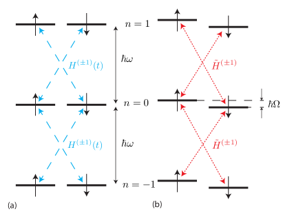
Figure 4: A Floquet picture for a spin $1/2$ system in an oscillating magnetic field with a slowly rotating direction $\mathbf{B}\left(t\right)=B\left[\cos\left(\Omega t\right)\mathbf{e}_{x}+\sin\left(\Omega t\right)\mathbf{e}_{y}\right]$ in the laboratory (a) and rotating (b) frames. Dotted (red) arrows represent quantum jumps between different Floquet bands in the rotating frame described by the operators $\tilde{H}^{\left(\pm 1\right)}=g_{F}BF_{1}/2$. Dashed (blue) arrows represent the corresponding quantum jumps in the laboratory frame described by the time-dependent operator $H^{\left(\pm 1\right)}=g_{F}B\left[F_{1}\cos\left(\Omega t\right)+F_{2}\sin\left(\Omega t\right)\right]$ . The transition from the laboratory to the rotating frames introduces a splitting of the spin-up and -down states by the amount $\hbar\Omega$, as illustrated in (b). This leads to the second-order correction to the Zeeman term given by Eq. (93c).

Alternatively, one can apply to the original Hamiltonian $H\left(\omega t+\theta,t\right)$ a unitary transformation $U_{\Omega t}=e^{-\frac{i}{\hbar}F_{3}\Omega t}$ rotating the spin along the $z$ axes by the angle $\Omega t$. The transformed Hamiltonian then reads as

$$\tilde{H}\left(\omega t+\theta,t\right) =U_{\Omega t}^{\dagger}HU_{\Omega t}-i\hbar U_{\Omega t}^{\dagger}\dot{U}_{\Omega t}$$ (92)

$$=g_{F}F_{1}B\cos\left(\omega t+\theta\right)-F_{3}\Omega\,.$$

Therefore, in the new frame the oscillating magnetic field vector is oriented in the $x$ direction and thus no longer rotates. Additionally, a Zeeman term $-F_{3}\Omega$ appears due to the rotational frequency shift Bialynicki-Birula and Bialynicka-Birula (1997). This is illustrated in Fig. 4 for a spin-$1/2$ case. Non-zero Fourier components of the transformed Hamiltonian are $\tilde{H}^{\left(0\right)}=-F_{3}\Omega$ and $\tilde{H}^{\left(-1\right)}=\tilde{H}^{\left(1\right)}=g_{F}F_{1}B/2$. Therefore a high frequency expansion of the effective Hamiltonian $\tilde{H}_{\textrm{eff}}$ reads in the rotating frame using Eqs. (33)

$$\tilde{H}_{\textrm{eff}\left(0\right)}= -F_{3}\Omega,$$ (93a)

$$\tilde{H}_{\textrm{eff}\left(1\right)}= \mathbf{0}_{\mathscr{H}},$$ (93b)

$$\tilde{H}_{\textrm{eff}\left(2\right)}= \frac{1}{\left(\hbar\omega\right)^{2}}\left[\tilde{H}^{\left(1\right)},\left[\tilde{H}^{\left(0\right)},\tilde{H}^{\left(1\right)}\right]\right]=\frac{g_{F}^{2}B^{2}\Omega}{4\omega^{2}}F_{3}.$$ (93c)

The second order term $\tilde{H}_{\textrm{eff}\left(2\right)}$ in Eq. (93c) represents a correction to the rotational energy shift. The term $\tilde{H}_{\textrm{eff}\left(2\right)}$ coincides with Eq. (91) for the shift in the laboratory frame due to the changes in the direction of the oscillating magnetic field. Yet in the rotating frame the effective Hamiltonian $\tilde{H}_{\textrm{eff}}$ also acquires the zero order term $\tilde{H}_{\textrm{eff}\left(0\right)}$ given by Eq. (93a), which is absent in the laboratory frame. To eliminate $\tilde{H}_{\textrm{eff}\left(0\right)}$ one needs to return back to the laboratory frame, giving

$$U_{\Omega t}\tilde{H}_{\textrm{eff}}U_{\Omega t}^{\dagger}-i\hbar U_{\Omega t}\dot{U}_{\Omega t}^{\dagger}=\tilde{H}_{\textrm{eff}\left(2\right)}\,,$$ (94)

which is in agreement with Eq. (91) for $H_{\textrm{eff}}$. Thus one arrives at completely equivalent effective Hamiltonians using both approaches.

References

- Oka and Aoki (2009) T. Oka and H. Aoki, Phys. Rev. B 79, 081406(R) (2009).
- Kitagawa et al. (2010) T. Kitagawa, E. Berg, M. Rudner, and E. Demler, Phys. Rev. B 82, 235114 (2010).
- Lindner et al. (2011) N. H. Lindner, G. Refael, and V. Galitski, Nat. Phys. 7, 490 (2011).
- Ho and Gong (2012) D. Y. H. Ho and J. Gong, Phys. Rev. Lett. 109, 010601 (2012).
- Hauke et al. (2014) P. Hauke, M. Lewenstein, and A. Eckardt, Phys. Rev. Lett. 113, 045303 (2014).
- Rudner et al. (2013) M. S. Rudner, N. H. Lindner, E. Berg, and M. Levin, Phys. Rev. X 3, 031005 (2013).
- Miyake et al. (2013) H. Miyake, G. A. Siviloglou, C. J. Kennedy, W. C. Burton, and W. Ketterle, Phys. Phys. Lett. 111, 185302 (2013).
- Aidelsburger et al. (2013) M. Aidelsburger, M. Atala, M. Lohse, J. T. Barreiro, B. Paredes, and I. Bloch, Phys. Rev. Lett. 111, 185301 (2013).
- Jotzu et al. (2014) G. Jotzu, M. Messer, R. Desbuquois, M. Lebrat, T. Uehlinger, D. Greif, and T. Esslinger, Nature 515, 237 (2014).
- Fregoso et al. (2013) B. M. Fregoso, Y. H. Wang, N. Gedik, and V. Galitski, Phys. Rev. B 88, 155129 (2013).
- Grushin et al. (2014) A. G. Grushin, A. Gómez-León, and T. Neupert, Phys. Rev. Lett. 112, 156801 (2014).
- Aidelsburger et al. (2015) M. Aidelsburger, M. Lohse, C. Schweizer, M. Atala, J. T. Barreiro, S. Nascimbène, N. R. Cooper, I. Bloch, and N. Goldman, Nat. Phys. 11, 162 (2015).
- Baur et al. (2014) S. K. Baur, M. H. Schleier-Smith, and N. R. Cooper, Phys. Rev. A 89, 051605(R) (2014).
- Zheng and Zhai (2014) W. Zheng and H. Zhai, Phys. Rev. A 89, 061603(R) (2014).
- Zhang and Zhou (2014) S.-L. Zhang and Q. Zhou, Phys. Rev. A 90, 051601(R) (2014).
- Mei et al. (2014) F. Mei, J.-B. You, D.-W. Zhang, X. C. Yang, R. Fazio, S.-L. Zhu, and L. C. Kwek, Phys. Rev. A 90, 063638 (2014).
- Anisimovas et al. (2015) E. Anisimovas, G. Žlabys, B. M. Anderson, G. Juzeliūnas, and A. Eckardt, Phys. Rev. B 91, 245135 (2015).
- Zheng et al. (2015) Z. Zheng, C. Qu, X. Zou, and C. Zhang, Phys. Rev. A 91, 063626 (2015).
- Verdeny and Mintert (2015) A. Verdeny and F. Mintert, Phys. Rev. A 92, 063615 (2015).
- Przysiężna et al. (2015) A. Przysiężna, O. Dutta, and J. Zakrzewski, New. J. Phys. 17, 013018 (2015).
- (21) O. Dutta, L. Tagliacozzo, M. Lewenstein, and J. Zakrzewski, “Toolbox for Abelian lattice gauge theories with synthetic matter,” arXiv:1601.03303 [cond-mat.quant-gas] .
- Xiong et al. (2016) T.-S. Xiong, J. Gong, and J.-H. An, Phys. Rev. B 93, 184306 (2016).
- Bomantara et al. (2016) R. W. Bomantara, G. N. Raghava, L. Zhou, and J. Gong, Phys. Rev. E 93, 022209 (2016).
- (24) K. Plekhanov, G. Roux, and K. Le Hur, “Floquet engineering of Haldane Chern insulators and chiral bosonic phase transitions,” arXiv:1608.00025 [cond-mat.quant-gas] .
- Fläschner et al. (2016) N. Fläschner, B. S. Rem, M. Tarnowski, D. Vogel, D.-S. Lühmann, K. Sengstock, and C. Weitenberg, Science 352, 1091 (2016).
- (26) N. Fläschner, D. Vogel, M. Tarnowski, B. S. Rem, D.-S. Lühmann, M. Heyl, J. C. Budich, L. Mathey, K. Sengstock, and C. Weitenberg, “Observation of a dynamical topological phase transition,” arXiv:1608.05616 [cond-mat.quant-gas] .
- Sørensen et al. (2005) A. S. Sørensen, E. Demler, and M. D. Lukin, Phys. Rev. Lett. 94, 086803 (2005).
- Eckardt et al. (2005) A. Eckardt, C. Weiss, and M. Holthaus, Phys. Rev. Lett. 95, 260404 (2005).
- Zenesini et al. (2009) A. Zenesini, H. Lignier, D. Ciampini, O. Morsch, and E. Arimondo, Phys. Rev. Lett. 102, 100403 (2009).
- Eckardt et al. (2010) A. Eckardt, P. Hauke, P. Soltan-Panahi, C. Becker, K. Sengstock, and M. Lewenstein, Europhys. Lett. 89, 10010 (2010).
- Neupert et al. (2011) T. Neupert, L. Santos, C. Chamon, and C. Mudry, Phys. Rev. Lett. 106, 236804 (2011).
- Regnault and Bernevig (2011) N. Regnault and B. A. Bernevig, Phys. Rev. X 1, 021014 (2011).
- Struck et al. (2011) J. Struck, C. Ölschläger, R. Le Targat, P. Soltan-Panahi, A. Eckardt, M. Lewenstein, P. Windpassinger, and K. Sengstock, Science 333, 996 (2011).
- Wu et al. (2012) Y.-L. Wu, B. A. Bernevig, and N. Regnault, Phys. Rev. B 85, 075116 (2012).
- Lewenstein et al. (2012) M. Lewenstein, A. Sanpera, and V. Ahufinger, Ultracold atoms in optical lattices: simulating quantum many-body systems (Oxford University Press, 2012).
- Struck et al. (2013) J. Struck, M. Weinberg, C. Ölschläger, P. Windpassinger, J. Simonet, K. Sengstock, R. Höppner, P. Hauke, A. Eckardt, M. Lewenstein, and L. Mathey, Nat. Phys. 9, 738 (2013).
- Bergholtz and Liu (2013) E. J. Bergholtz and Z. Liu, Int. J. Mod. Phys. B 27, 1330017 (2013).
- Parameswaran et al. (2013) S. A. Parameswaran, R. Roy, and S. L. Sondhi, C. R. Phys. 14, 816 (2013).
- Greschner et al. (2014) S. Greschner, G. Sun, D. Poletti, and L. Santos, Phys. Phys. Lett. 113, 215303 (2014).
- Račiūnas et al. (2016) M. Račiūnas, G. Žlabys, A. Eckardt, and E. Anisimovas, Phys. Rev. A 93, 043618 (2016).
- Meinert et al. (2016) F. Meinert, M. J. Mark, K. Lauber, A. J. Daley, and H.-C. Nägerl, Phys. Rev. Lett. 116, 205301 (2016).
- (42) A. Eckardt, “Atomic quantum gases in periodically driven optical lattices,” arXiv:1606.08041 [cond-mat.quant-gas] .
- Arimondo et al. (2012) E. Arimondo, D. Ciampini, A. Eckardt, M. Holthaus, and O. Morsch, Adv. At. Molec. Opt. Phys. 61, 515 (2012).
- Windpassinger and Sengstock (2013) P. Windpassinger and K. Sengstock, Rep. Progr. Phys. 76, 086401 (2013).
- Goldman and Dalibard (2014) N. Goldman and J. Dalibard, Phys. Rev. X 4, 031027 (2014).
- Goldman et al. (2014) N. Goldman, G. Juzeliūnas, P. Öhberg, and I. B. Spielman, Rep. Progr. Phys. 77, 126401 (2014).
- Bukov et al. (2015) M. Bukov, L. D’Alessio, and A. Polkovnikov, Adv. Phys. 64, 139 (2015).
- Goldman et al. (2015) N. Goldman, J. Dalibard, M. Aidelsburger, and N. R. Cooper, Phys. Rev. A 91, 033632 (2015).
- Eckardt and Anisimovas (2015) A. Eckardt and E. Anisimovas, New J. Phys. 17, 093039 (2015).
- Itin and Katsnelson (2015) A. P. Itin and M. I. Katsnelson, Phys. Rev. Lett. 115, 075301 (2015).
- Mikami et al. (2016) T. Mikami, S. Kitamura, K. Yasuda, N. Tsuji, T. Oka, and H. Aoki, Phys. Rev. B 93, 144307 (2016).
- Holthaus (2016) M. Holthaus, J. Phys. B: At. Mol. Opt. Phys. 49, 013001 (2016).
- Hemmerich (2010) A. Hemmerich, Phys. Rev. A 81, 063626 (2010).
- Kolovsky (2011) A. R. Kolovsky, Europhys. Lett. 93, 20003 (2011).
- Creffield and Sols (2013) C. E. Creffield and F. Sols, Europhys. Lett. 101, 40001 (2013).
- Creffield and Sols (2014) C. E. Creffield and F. Sols, Phys. Rev. A 90, 023636 (2014).
- Hauke et al. (2012) P. Hauke, O. Tieleman, A. Celi, C. Ölschläger, J. Simonet, J. Struck, M. Weinberg, P. Windpassinger, K. Sengstock, M. Lewenstein, and A. Eckardt, Phys. Rev. Lett. 109, 145301 (2012).
- Iadecola and Chamon (2015) T. Iadecola and C. Chamon, Phys. Rev. B 91, 184301 (2015).
- Jiménez-García et al. (2015) K. Jiménez-García, L. J. LeBlanc, R. A. Williams, M. C. Beeler, C. Qu, M. Gong, C. Zhang, and I. B. Spielman, Phys. Rev. Lett. 114, 125301 (2015).
- Heinisch and Holthaus (2016) C. Heinisch and M. Holthaus, J. Mod. Opt. 63, 1768 (2016).
- Kitagawa et al. (2011) T. Kitagawa, T. Oka, A. Brataas, L. Fu, and E. Demler, Phys. Rev. B 84, 235108 (2011).
- Tong et al. (2013) Q.-J. Tong, J.-H. An, J. Gong, H.-G. Luo, and C. H. Oh, Phys. Rev. B 87, 201109(R) (2013).
- Usaj et al. (2014) G. Usaj, P. M. Perez-Piskunow, L. E. F. Foa Torres, and C. A. Balseiro, Phys. Rev. B 90, 115423 (2014).
- Quelle et al. (2015) A. Quelle, W. Beugeling, and C. Morais Smith, Solid St. Commun. 215-216, 27 (2015).
- Haldane and Raghu (2008) F. D. M. Haldane and S. Raghu, Phys. Rev. Lett. 100, 013904 (2008).
- Rechtsman et al. (2013) M. C. Rechtsman, J. M. Zeuner, Y. Plotnik, Y. Lumer, D. Podolsky, F. Dreisow, S. Nolte, M. Segev, and A. Szameit, Nature 496, 196 (2013).
- Dalibard et al. (2011) J. Dalibard, F. Gerbier, G. Juzeliūnas, and P. Öhberg, Rev. Mod. Phys. 83, 1523 (2011).
- Aidelsburger et al. (2011) M. Aidelsburger, M. Atala, S. Nascimbène, S. Trotzky, Y.-A. Chen, and I. Bloch, Phys. Rev. Lett. 107, 255301 (2011).
- Atala et al. (2014) M. Atala, M. Aidelsburger, M. Lohse, J. T. Barreiro, B. Paredes, and I. Bloch, Nat. Phys. 10, 588 (2014).
- Struck et al. (2012) J. Struck, C. Ölschläger, M. Weinberg, P. Hauke, J. Simonet, A. Eckardt, M. Lewenstein, K. Sengstock, and P. Windpassinger, Phys. Rev. Lett. 108, 225304 (2012).
- Kennedy et al. (2015) C. J. Kennedy, W. C. Burton, W. C. Chung, and W. Ketterle, Nat. Phys. 11, 859 (2015).
- (72) J. C. Budich, Y. Hu, and P. Zoller, “Helical Floquet channels in 1D lattices,” arXiv:1608.05096 .
- Galitski and Spielman (2013) V. Galitski and I. B. Spielman, Nature 494, 49 (2013).
- Zhai (2012) H. Zhai, Int. J. Mod. Phys. B 26, 1230001 (2012).
- Zhai (2015) H. Zhai, Rep. Prog. Phys. 78, 026001 (2015).
- Anderson et al. (2013) B. M. Anderson, I. B. Spielman, and G. Juzeliūnas, Phys. Rev. Lett. 111, 125301 (2013).
- Xu et al. (2013) Z.-F. Xu, L. You, and M. Ueda, Phys. Rev. A 87, 063634 (2013).
- Nascimbene et al. (2015) S. Nascimbene, N. Goldman, N. R. Cooper, and J. Dalibard, Phys. Rev. Lett. 115, 140401 (2015).
- Perez-Piskunow et al. (2015) P. M. Perez-Piskunow, L. E. F. Foa Torres, and G. Usaj, Phys. Rev. A 91, 043625 (2015).
- Luo et al. (2016) X. Luo, L. Wu, J. Chen, Q. Guan, K. Gao, Z.-F. Xu, L. You, and R. Wang, Sci. Rep. 6, 18983 (2016).
- Rahav et al. (2003) S. Rahav, I. Gilary, and S. Fishman, Phys. Rev. A 68, 013820 (2003).
- Guérin and Jauslin (2003) S. Guérin and H. R. Jauslin, Adv. Chem. Phys. 125, 147 (2003).
- Sambe (1973) H. Sambe, Phys. Rev. A 7, 2203 (1973).
- Howland (1974) J. S. Howland, Mathematische Annalen 207, 315 (1974).
- Breuer and Holthaus (1989a) H. P. Breuer and M. Holthaus, Z. Phys. D 11, 1 (1989a).
- Breuer and Holthaus (1989b) H. P. Breuer and M. Holthaus, Phys. Lett. A 140, 507 (1989b).
- Grifoni and Hänggi (1998) M. Grifoni and P. Hänggi, Phys. Rep. 304, 229 (1998).
- Drese and Holthaus (1999) K. Drese and M. Holthaus, Eur. Phys. J. D 5, 119 (1999).
- Eckardt and Holthaus (2008) A. Eckardt and M. Holthaus, Phys. Rev. Lett. 101, 245302 (2008).
- Note (1) Subsequently in Eq. (15) we shall adopt such a -independent initial condition.
- Peskin and Moiseyev (1993) U. Peskin and N. Moiseyev, J. Chem. Phys. 99, 4590 (1993).
- Fleischer and Moiseyev (2005) A. Fleischer and N. Moiseyev, Phys. Rev. A 72, 032103 (2005).
- (93) P. Weinberg, M. Bukov, L. D’Alessio, A. Polkovnikov, S. Vajna, and M. Kolodrubetz, “Adiabatic perturbation theory and geometry of periodically-driven systems,” arXiv:1606.02229 .
- Berry (1984) M. Berry, Proc. R. Soc. A 392, 45 (1984).
- Mead (1992) C. A. Mead, Rev. Mod. Phys. 64, 51 (1992).
- Note (2) Previously the notion of time-dependent effective Hamiltonians was used in the Supplementary material of Ref. Nascimbene et al. (2015) to describe a slow ramp of a dynamical optical lattice with a sub-wavelength spacing. The ramp was split into a set of stroboscopic pieces, in which the modulation was assumed to be constant in amplitude. In such an approach, the obtained time-dependent effective Hamiltonian contains a contribution that depends on the initial phase of the drive. However, this should not be considered as a genuine contribution to the effective Hamiltonian. The latter is associated with a long-time dynamics and should be independent of the initial phase, as in the case of the stationary driving Rahav et al. (2003); Goldman and Dalibard (2014); Eckardt and Anisimovas (2015).
- Kuwahara et al. (2016) T. Kuwahara, T. Mori, and K. Saito, Ann. Phys. 367, 96 (2016).
- Hone et al. (1997) D. W. Hone, R. Ketzmerick, and W. Kohn, Phys. Rev. A 56, 4045 (1997).
- Wilczek and Zee (1984) F. Wilczek and A. Zee, Phys. Rev. Lett. 52, 2111 (1984).
- Moody et al. (1986) J. Moody, A. Shapere, and F. Wilczek, Phys. Rev. Lett. 56, 893 (1986).
- Zee (1988) A. Zee, Phys. Rev. A 38, 1 (1988).
- Lignier et al. (2007) H. Lignier, C. Sias, D. Ciampini, Y. Singh, A. Zenesini, O. Morsch, and E. Arimondo, Phys. Rev. Lett. 99, 220403 (2007).
- Bialynicki-Birula and Bialynicka-Birula (1997) I. Bialynicki-Birula and Z. Bialynicka-Birula, Phys. Rev. Lett. 78, 2539 (1997).
- Ben Dahan et al. (1996) M. Ben Dahan, E. Peik, J. Reichel, Y. Castin, and C. Salomon, Phys. Rev. Lett. 76, 4508 (1996).
- Madison et al. (1997) K. Madison, C. Bharucha, P. Morrow, S. Wilkinson, Q. Niu, B. Sundaram, and M. Raizen, Applied Physics B 65, 693 (1997).
- Madison et al. (1998) K. W. Madison, M. C. Fischer, R. B. Diener, Q. Niu, and M. G. Raizen, Phys. Rev. Lett. 81, 5093 (1998).
- Niu et al. (1996) Q. Niu, X.-G. Zhao, G. A. Georgakis, and M. G. Raizen, Phys. Rev. Lett. 76, 4504 (1996).
- Sias et al. (2008) C. Sias, H. Lignier, Y. P. Singh, A. Zenesini, D. Ciampini, O. Morsch, and E. Arimondo, Phys. Rev. Lett. 100, 040404 (2008).