SISSA 48/2016/FISI

IPMU16-0125

TTP16-035

Renormalisation Group Corrections to
Neutrino Mixing Sum Rules

J. Gehrlein${}^{\,a,}$ , S. T. Petcov${}^{\,b,c,}$ , M. Spinrath${}^{\,a,}$ , A. V. Titov${}^{\,b,}$

^a Institut für Theoretische Teilchenphysik, Karlsruhe Institute of Technology,

Engesserstraße 7, D-76131 Karlsruhe, Germany

^b SISSA/INFN, Via Bonomea 265, I-34136 Trieste, Italy

^c Kavli IPMU (WPI), University of Tokyo,

5-1-5 Kashiwanoha, 277-8583 Kashiwa, Japan

Neutrino mixing sum rules are common to a large class of models based on the (discrete) symmetry approach to lepton flavour. In this approach the neutrino mixing matrix $U$ is assumed to have an underlying approximate symmetry form $\tilde{U}_{\nu}$, which is dictated by, or associated with, the employed (discrete) symmetry. In such a setup the cosine of the Dirac CP-violating phase $\delta$ can be related to the three neutrino mixing angles in terms of a sum rule which depends on the symmetry form of $\tilde{U}_{\nu}$. We consider five extensively discussed possible symmetry forms of $\tilde{U}_{\nu}$: i) bimaximal (BM) and ii) tri-bimaximal (TBM) forms, the forms corresponding to iii) golden ratio type A (GRA) mixing, iv) golden ratio type B (GRB) mixing, and v) hexagonal (HG) mixing. For each of these forms we investigate the renormalisation group corrections to the sum rule predictions for $\delta$ in the cases of neutrino Majorana mass term generated by the Weinberg (dimension 5) operator added to i) the Standard Model, and ii) the minimal SUSY extension of the Standard Model.

1 Introduction

Understanding the observed pattern of neutrino mixing and establishing the status of leptonic CP violation are among the “big” open questions in particle physics. Considerable efforts have been made in the past years trying to answer these fundamental questions. In particular, the approach based on a discrete non-Abelian family symmetry in the lepton sector, assumed to be existing at some high-energy scale, has been widely studied in the literature (for reviews on the subject see [1, 2, 3, 4]). In this approach the family symmetry has necessarily to be broken at low energies to some residual symmetries of the charged lepton and neutrino mass matrices. These residual symmetries constrain the form of the matrices which diagonalise the charged lepton and neutrino mass matrices, and hence the form of the Pontecorvo, Maki, Nakagawa, Sakata (PMNS) neutrino mixing matrix.

In the three neutrino mixing case (see, e.g., [5]) the $3\times 3$ unitary PMNS matrix can be parametrised in terms of three mixing angles, $\theta_{12}$, $\theta_{13}$, $\theta_{23}$, one Dirac phase $\delta$ and, if the massive neutrinos are Majorana particles, two Majorana phases [6]. The Dirac and Majorana phases are responsible for CP violation in the lepton sector. The neutrino mixing parameters $\sin^{2}\theta_{12}$, $\sin^{2}\theta_{13}$ and $\sin^{2}\theta_{23}$ have been determined with a relatively high precision in the recent global analyses [7, 8, 9]. These analyses provided only a hint so far that $\delta\approx 3\pi/2$. In Table 1 we summarise the best fit values, $1\sigma$ and $3\sigma$ allowed ranges of the mixing parameters and the mass squared differences $\Delta m_{21}^{2}$ and $\Delta m_{31}^{2}$ ($\Delta m_{23}^{2}$), with $\Delta m_{ij}^{2}\equiv m_{i}^{2}-m_{j}^{2}$, $m_{1,2,3}$ being the neutrino masses, found in ref. [7] for the neutrino mass spectrum with normal (inverted) ordering (denoted further as the NO (IO) spectrum). We will use the results given in Table 1 in our numerical analyses.

Parameter	Best fit	$1\sigma$ range	$3\sigma$ range
$\sin^{2}\theta_{12}/10^{-1}$	$2.97$	$2.81\rightarrow 3.14$	$2.50\rightarrow 3.54$
$\sin^{2}\theta_{13}/10^{-2}$ (NO)	$2.14$	$2.05\rightarrow 2.25$	$1.85\rightarrow 2.46$
$\sin^{2}\theta_{13}/10^{-2}$ (IO)	$2.18$	$2.06\rightarrow 2.27$	$1.86\rightarrow 2.48$
$\sin^{2}\theta_{23}/10^{-1}$ (NO)	$4.37$	$4.17\rightarrow 4.70$	$3.79\rightarrow 6.16$
$\sin^{2}\theta_{23}/10^{-1}$ (IO)	$5.69$	$4.28\rightarrow 4.91\oplus 5.18\rightarrow 5.97$	$3.83\rightarrow 6.37$
$\delta/\pi$ (NO)	$1.35$	$1.13\rightarrow 1.64$	$0\rightarrow 2$
$\delta/\pi$ (IO)	$1.32$	$1.07\rightarrow 1.67$	$0\rightarrow 2$
$\Delta m_{21}^{2}/10^{-5}$ eV2	$7.37$	$7.21\rightarrow 7.54$	$6.93\rightarrow 7.97$
$\Delta m_{31}^{2}/10^{-3}$ eV2 (NO)	$2.54$	$2.50\rightarrow 2.58$	$2.40\rightarrow 2.67$
$\Delta m_{23}^{2}/10^{-3}$ eV2 (IO)	$2.50$	$2.46\rightarrow 2.55$	$2.36\rightarrow 2.64$

Table 1: The best fit values, $1\sigma$ and 3$\sigma$ ranges of the neutrino oscillation parameters taken from [7].

In the discrete symmetry approach specific correlations between the mixing angles and the CP-violating (CPV) phases occur. These correlations are usually referred to as neutrino mixing sum rules (see, e.g., [3, 4, 10, 11, 12, 13, 14, 15, 16, 17]). Since mixing sum rules are concrete relations between different observables, i.e., the neutrino mixing angles and the Dirac phase, they can be tested experimentally. Thus, via sum rules, one can examine the current phenomenologically viable flavour models based on different discrete symmetries.

In [12, 15] different mixing sum rules have been derived and in [13, 15, 14] the phenomenological consequences of these sum rules have been studied. In [16] sum rules and predictions for $\cos\delta$ have been obtained from different types of residual symmetries in the charged lepton and neutrino sectors. In these studies it was assumed that the sum rule is exactly realised at low energy. However, as every quantity in quantum field theory, the mixing parameters get affected by renormalisation group (RG) running. Similar to the study of renormalisation group corrections to neutrino mass sum rules in [19], we investigate in the present article the impact of corrections from the renormalisation group equations (RGEs) on the mixing sum rule predictions for the Dirac phase $\delta$. The main question we want to address is how stable the predictions for $\delta$ are under RG corrections which under certain conditions can be expected to be quite sizeable [20].

In the literature RG corrections to certain type of mixing sum rules have been studied before. The first attempt to study RG corrections to mixing angle sum rules, to our knowledge, has been made in [21] for the quark-lepton complementarity relations, $\theta_{12}+\theta_{C}\cong\pi/4$ and $\theta_{23}+\arcsin\,V_{cb}\cong\pi/4$, $\theta_{C}$ and $V_{cb}$ being the Cabibbo angle and an element of the Cabibbo, Kobayashi, Maskawa (CKM) quark mixing matrix. In [22] the RG corrections for the sum rule relating the element $U_{\tau e}$ of the PMNS matrix to the element $V^{\rm TBM}_{\tau e}=-\,1/\sqrt{6}$ of the tri-bimaximal mixing matrix, $|U_{\tau e}|=1/\sqrt{6}$, and for the leading order in $\theta_{13}$ versions of this sum rule, have been investigated. In refs. [21] and [22] the bimaximal (BM) mixing [23] scheme and the tri-bimaximal (TBM) mixing scheme [24] (see also [25]) , respectively, were analysed. In [26] the study of RG perturbations was done for an approximate (leading order) mixing sum rule and for normal hierarchical neutrino mass spectrum, $m_{1}\ll m_{2}<m_{3}$, neglecting terms of order $\mathcal{O}(m_{1}/m_{2})$ and $\mathcal{O}(m_{1}/m_{3})$. The authors of [26] extended their analysis to incorporate canonical normalisation effects besides RG corrections. Both type of corrections were assumed to be dominated by the third family effects. The authors of [27] estimated the size of RG corrections to the sum rules we will be considering in the present study by taking into account only the RG correction to $\theta_{12}$.

In the present article we go beyond these previous works i) by considering the exact form of the general mixing sum rules derived in [12], ii) by taking into account the RG corrections not only to the angle $\theta_{12}$, but to all three neutrino mixing angles $\theta_{12}$, $\theta_{23}$, $\theta_{13}$ and the CPV phases, iii) discussing not only the cases of BM or TBM mixing schemes, but also the cases of golden ratio type A (GRA) [28], golden ratio type B (GRB) [29] and hexagonal (HG) [30] mixing schemes, and iv) by considering both the cases of NO and IO neutrino mass spectra. We perform the analysis assuming that the neutrino Majorana mass matrix is generated by the Weinberg (dimension 5) operator. The RG corrections to the sum rules of interest are calculated in the Standard Model as well as in the minimal supersymmetric extension of the Standard Model (MSSM).

Our study goes also beyond [31] where only the GRA, BM and TBM mixing schemes were analysed. We discuss different forms of the charged lepton mixing matrix and present a significantly larger number of results. In particular, we derive values of the neutrino mass scale and $\tan\beta$ for which the various mixing schemes are still viable. We make a thorough numerical analysis from which we derive likelihood functions for the value of the Dirac CPV phase $\delta$ at low energies if the specified mixing sum rule holds at high energies.

The paper is organised as follows: after a short review of the framework for mixing sum rules in Section 2, we present analytical estimates for the allowed parameter regions for $\delta$ taking RG corrections into account in Section 3. In Section 4 we present the numerical results for the different mixing schemes. Finally, we summarise and conclude in Section 5 and present in the appendix plots for the likelihoods in terms of $\cos\delta$ for better comparison with previous literature.

2 Mixing Sum Rules

In this section we briefly review the framework in which mixing sum rules are obtained and fix notation and conventions. In the most general case the PMNS matrix $U$ can be parametrised as [32]

$$U=U_{e}^{\dagger}U_{\nu}=(\tilde{U}_{e})^{\dagger}\Psi\tilde{U}_{\nu}Q_{0}\,.$$ (2.1)

Here $U_{e}$ and $U_{\nu}$ are $3\times 3$ unitary matrices, which diagonalise, respectively, the charged lepton and neutrino mass matrices. $\tilde{U}_{e}$ and $\tilde{U}_{\nu}$ are CKM-like $3\times 3$ unitary matrices, and $\Psi$ and $Q_{0}$ are diagonal phase matrices:

$$\Psi =\text{diag}\left(1,\text{e}^{-\text{i}\,\psi},\text{e}^{-\text{i}\,\omega}\right)\,,$$ (2.2)

$$Q_{0} =\text{diag}\left(1,\text{e}^{\text{i}\tfrac{\xi_{21}}{2}},\text{e}^{\text{i}\tfrac{\xi_{31}}{2}}\right)\,.$$ (2.3)

The phases in $Q_{0}$ contribute to the Majorana phases in the PMNS matrix.

Similar to what has been done in [12, 13, 14, 15] we will consider the cases when $\tilde{U}_{\nu}$ has the BM, TBM, GRA, GRB and HG forms. For all these forms $\tilde{U}_{\nu}$ can be expressed as a product of $3\times 3$ orthogonal matrices $R_{23}$ and $R_{12}$ describing rotations in the 2-3 and 1-2 planes, i.e.,

$$\tilde{U}_{\nu}=R_{23}(\theta_{23}^{\nu})R_{12}(\theta_{12}^{\nu})\,,$$ (2.4)

with $\theta_{23}^{\nu}=-\pi/4$ and $\theta_{12}^{\nu}=\pi/4$ (BM); $\theta_{12}^{\nu}=\arcsin(1/\sqrt{3})$ (TBM); $\theta_{12}^{\nu}=\arctan(1/\phi)$ (GRA), $\phi=(1+\sqrt{5})/2$ being the golden ratio; $\theta_{12}^{\nu}=\arccos(\phi/2)$ (GRB); $\theta_{12}^{\nu}=\pi/6$ (HG). For convenience, in another convention the same list reads $\sin^{2}\theta_{23}^{\nu}=1/2$ and $\sin^{2}\theta_{12}^{\nu}=1/2$ (BM); $\sin^{2}\theta_{12}^{\nu}=1/3$ (TBM); $\sin^{2}\theta_{12}^{\nu}=(5-\sqrt{5})/10$ (GRA); $\sin^{2}\theta_{12}^{\nu}=(5-\sqrt{5})/8$ (GRB); $\sin^{2}\theta_{12}^{\nu}=1/4$ (HG).

For the matrix $\tilde{U}_{e}$, following [12], we will consider two different forms both of which correspond to negligible $\theta^{e}_{13}$. They are realised in a class of flavour models based on a GUT and/or a discrete symmetry (see, e.g., [33, 34, 35, 36, 39, 37, 38]). The first form is characterised also by zero $\theta^{e}_{23}$, i.e.,

$$\tilde{U}_{e}=R_{12}^{-1}(\theta^{e}_{12})\,.$$ (2.5)

In this case there is a correlation between the values of $\sin^{2}\theta_{23}$ and $\sin^{2}\theta_{13}$:

$$\sin^{2}\theta_{23}=\frac{\sin^{2}\theta^{\nu}_{23}-\sin^{2}\theta_{13}}{1-\sin^{2}\theta_{13}}\,,$$ (2.6)

which for all the symmetry forms of $\tilde{U}_{\nu}$ introduced above leads to

$$\sin^{2}\theta_{23}=\frac{1-2\sin^{2}\theta_{13}}{2\,(1-\sin^{2}\theta_{13})}=\frac{1}{2}-\frac{1}{2}\sin^{2}\theta_{13}+\mathcal{O}(\sin^{4}\theta_{13})\,.$$ (2.7)

This implies in turn that $\theta_{23}$ cannot deviate significantly from $\pi/4$. The second form of $\tilde{U}_{e}$ corresponds to non-zero $\theta^{e}_{12}$ and $\theta^{e}_{23}$, i.e.,

$$\tilde{U}_{e}=R_{23}^{-1}(\theta_{23}^{e})R_{12}^{-1}(\theta_{12}^{e})\,.$$ (2.8)

This matrix provides the corrections to $\tilde{U}_{\nu}$ necessary to reproduce the current best fit values of all the three neutrino mixing angles $\theta_{12}$, $\theta_{13}$ and $\theta_{23}$ in the PMNS matrix $U$ without any further contributions like RG or other corrections.

It was shown in [12] that for $\tilde{U}_{\nu}$ given in eq. (2.4) and $\tilde{U}_{e}$ determined in eqs. (2.5) or (2.8), the Dirac phase $\delta$ present in the PMNS matrix satisfies a sum rule which reads

$$\cos\delta=\frac{\tan\theta_{23}}{\sin 2\theta_{12}\sin\theta_{13}}\left[\cos 2\theta_{12}^{\nu}+\left(\sin^{2}\theta_{12}-\cos^{2}\theta_{12}^{\nu}\right)\left(1-\text{cot}^{2}\theta_{23}\sin^{2}\theta_{13}\right)\right]\,.$$ (2.9)

Additionally, in the case of $\tilde{U}_{e}$ given in eq. (2.5), the correlation between $\theta_{23}$ and $\theta_{13}$, eq. (2.7), has to be respected. The sum rule, eq. (2.9), in this case reduces to [12]

$$\cos\delta=\frac{(1-2\sin^{2}\theta_{13})^{\frac{1}{2}}}{\sin 2\theta_{12}\sin\theta_{13}}\,\bigg{[}\cos 2\theta^{\nu}_{12}+\left(\sin^{2}\theta_{12}-\cos^{2}\theta^{\nu}_{12}\right)\,\frac{1-3\sin^{2}\theta_{13}}{1-2\sin^{2}\theta_{13}}\bigg{]}\,.$$ (2.10)

In the following we will refer to the case with $\tilde{U}_{e}$ given in eq. (2.5) (eq. (2.8)) as to the case of zero (non-zero) $\theta^{e}_{23}$. In this article we will study the impact of the RG corrections on the mixing sum rules in eqs. (2.9) and (2.10), and the angle sum rule in eq. (2.7), which are assumed to hold at some high-energy scale specified later.

In [15] other forms of the matrices $\tilde{U}_{e}$ and $\tilde{U}_{\nu}$ corresponding to different rotations and leading to sum rules for $\cos\delta$ of the type of eqs. (2.9) and (2.10) have been investigated. The RG corrections to them, however, are expected to be similar to the ones which take place for the sum rules described above. For this reason we will not consider them in the present study.

3 Analytical Estimates

Before we present our numerical results in the next section, we give in this section analytical estimates of the effect of radiative corrections on the mixing sum rules. We discuss how we obtain constraints on the mass scale and on $\tan\beta$ (in the MSSM) from the requirement that the mixing sum rule has to be fulfilled at the high scale.

3.1 General Effects of Radiative Corrections

The running of the mixing parameters is already known for quite some time, see, e.g., [20]. One might wonder if RG corrections have a large impact on the predicted value for $\delta$ from the sum rule in eq. (2.9). Indeed, we expect large RG corrections for a large Yukawa coupling (large $\tan\beta$) and a heavy neutrino mass scale. To be more precise, the $\beta$-functions of the mixing angles, in the leading order in $\theta_{13}$ and neglecting the electron and muon Yukawa couplings in comparison to the tau one, depend on the tau Yukawa coupling, the absolute neutrino mass scale (or ${\rm min}(m_{j})$, $j=1,2,3$), the mixing angles, the type of spectrum – normal or inverted ordering – the neutrino masses obey, on the Majorana phases $\alpha_{1}$ and $\alpha_{2}$ , and in the MSSM – on $\tan\beta$. In the leading order in $\theta_{13}$ only the $\beta$-function for $\theta_{13}$ depends on $\delta$. The $\beta$-functions read up to $\mathcal{O}(\theta_{13})$ [20]:

$$\frac{\text{d}\,\theta_{12}}{\text{d}\,\ln(\mu/\mu_{0})} =-\frac{Cy_{\tau}^{2}}{32\pi^{2}}\sin 2\theta_{12}s^{2}_{23}\frac{\left|m_{1}\text{e}^{\text{i}\alpha_{1}}+m_{2}\text{e}^{\text{i}\alpha_{2}}\right|^{2}}{\Delta m_{21}^{2}}+\mathcal{O}(\theta_{13})\;,$$ (3.1)

$$\frac{\text{d}\,\theta_{13}}{\text{d}\,\ln(\mu/\mu_{0})} =\frac{Cy_{\tau}^{2}}{32\pi^{2}}\sin 2\theta_{12}\sin 2\theta_{23}\frac{m_{3}}{\Delta m_{32}^{2}(1+\zeta)}$$

$$\times\left[m_{1}\cos(\alpha_{1}-\delta)-(1+\zeta)m_{2}\cos(\alpha_{2}-\delta)-\zeta m_{3}\cos\delta\right]$$

$$+\mathcal{O}(\theta_{13})\;,$$ (3.2)

$$\frac{\text{d}\,\theta_{23}}{\text{d}\,\ln(\mu/\mu_{0})} =-\frac{Cy_{\tau}^{2}}{32\pi^{2}}\sin 2\theta_{23}\frac{1}{\Delta m_{32}^{2}}\left[c_{12}^{2}\left|m_{2}\text{e}^{\text{i}\alpha_{2}}+m_{3}\right|^{2}+s_{12}^{2}\frac{\left|m_{1}\text{e}^{\text{i}\alpha_{1}}+m_{3}\right|^{2}}{1+\zeta}\right]$$ (3.3)

$$+\mathcal{O}(\theta_{13})\;,$$

with $\mu$ being the renormalisation scale, $\zeta=\frac{\Delta m_{21}^{2}}{\Delta m_{32}^{2}}$ and $\frac{Cy_{\tau}^{2}}{32\pi^{2}}\approx 0.3\cdot 10^{-6}(1+\tan^{2}\beta)$ in the MSSM and $\frac{Cy_{\tau}^{2}}{32\pi^{2}}\approx-0.5\cdot 10^{-6}$ in the SM. In the SM there is no $\tan\beta$ enhancement and hence the effects are usually relatively small.

We would like to note at this point that we consider here only minimal scenarios, namely the SM and the MSSM augmented with Majorana neutrino masses. In standard seesaw scenarios it would be correct to integrate out the additional heavy states at their respective mass scale which would change the $\beta$-functions and the running. Nevertheless, we want to assume the heavy masses all to be roughly of the same order, so that it is a good approximation to impose the sum rules at the high scale and use the minimal $\beta$-functions for the running. For low scale seesaw mechanisms this would certainly be a bad approximation, but there the sum rule should be realised at the low scale as well and running effects can be more generally expected to be small.

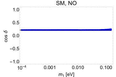
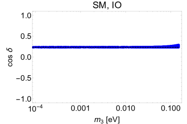
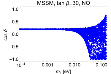
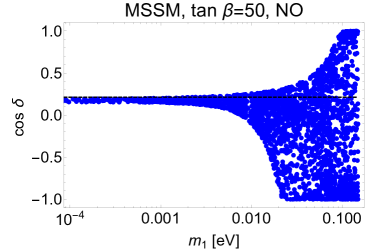
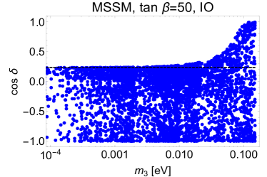
Figure 1: Results for the predicted value of $\cos\delta$ from the sum rule in eq. (2.9) for the GRA mixing scheme in the case where $\theta_{12}^{e}\neq 0$, $\theta_{23}^{e}\neq 0$ and $\theta_{13}^{e}=0$. The black dashed lines represent the tree level result. The blue points are our scan points. For the angles and the mass squared differences we took the best fit values from Table 1. We let the parameters run between the high-scale $M_{S}\approx 10^{13}$ GeV and the low-scale $M_{Z}$. The Majorana phases are chosen randomly between 0 and $2\pi$. The plots on the left (right) side correspond to normal (inverted) mass ordering.

To give an idea about the size of the effect of interest we show in Fig. 1 results for $\cos\delta$ as derived from the sum rule in eq. (2.9) for the GRA mixing scheme. We used the REAP package [40] to solve the RGEs for the mixing parameters between the low-energy scale $M_{Z}$ and the high-energy scale which we have set equal to the seesaw scale $M_{S}\approx 10^{13}$ GeV. We only consider the case with $\theta_{12}^{e}\neq 0$, $\theta_{23}^{e}\neq 0$ and $\theta_{13}^{e}=0$. We have set all mass squared differences and angles to their best fit values given in Table 1, scanned over the lightest neutrino mass and chose random values for the low energy Majorana phases. For the SM case we see no effect, while for $\tan\beta=30$ and 50, the RG effects are significant. Even for a moderate $\tan\beta$ in the MSSM and a relatively small mass scale $m_{\text{lightest}}\approx 0.04$ eV the effect is non-negligible. Since the running of the angles is stronger with an inverted mass ordering, the effect for the prediction of $\cos\delta$ is larger in the IO case. For that case it is furthermore in particular remarkable that the corrections do not go to zero for $m_{3}$ going to zero. This is due to the well-known fact, cf. [20], that the $\beta$-functions for $\delta$ and $\theta_{12}$ are in this limit enhanced by a factor of $\Delta m_{23}^{2}/\Delta m_{21}^{2}$. Together with the $\tan\beta$ enhancement this leads to quite sizeable effects for all relevant neutrino mass scales.

3.2 Allowed Parameter Regions with RG Corrections

In this subsection we derive constraints on $\tan\beta$ (in the case of the MSSM) and the mass of the lightest neutrino, $m_{\text{lightest}}$, by imposing the mixing sum rule at the high scale and by requiring that $\cos\delta\in[-1,1]$ at the high scale. We have chosen the high-scale to be equal to the seesaw scale $M_{S}\approx 10^{13}$ GeV. The BM mixing scheme is strongly disfavoured for the current best fit values of the neutrino mixing angles without taking the RG corrections into account. Thus, one of the questions we are interested in is whether the corrections can reconstitute the validity of the BM scheme even for the best fit values of the angles.

We give first analytical estimates of the RG effects on eq. (2.9). At the high scale we can write, for instance, for the mixing angles

$$\theta_{ij}(M_{S})=\theta_{ij}(M_{Z})+\delta\theta_{ij}\equiv\theta_{ij}+\delta\theta_{ij}\;,$$ (3.4)

where $\delta\theta_{ij}$ is the RG correction or the difference between the high-scale and low-scale values of the mixing angle $\theta_{ij}$. Since the RG corrections are small we can expand the mixing sum rule at the high-scale in the small quantities and find:

$$\cos\delta(M_{S})\approx \cos\delta(M_{Z})+\delta(\cos\delta)$$

$$=\frac{\tan\theta_{23}}{\sin 2\theta_{12}\sin\theta_{13}}(\cos 2\theta_{12}^{\nu}+(\sin^{2}\theta_{12}-\cos^{2}\theta_{12}^{\nu})(1-\text{cot}^{2}\theta_{23}\sin^{2}\theta_{13}))$$

$$+f_{13}(\theta_{13},\theta_{12},\theta_{23},\theta_{12}^{\nu})\,\delta\theta_{13}$$

$$+f_{23}(\theta_{13},\theta_{12},\theta_{23},\theta_{12}^{\nu})\,\delta\theta_{23}$$

$$+f_{12}(\theta_{13},\theta_{12},\theta_{23},\theta_{12}^{\nu})\,\delta\theta_{12}~{},$$ (3.5)

where the $f_{ij}$ are prefactors from the expansion. For the angles and mass squared differences at the low scale we use the best fit values. Note that the Dirac phase $\delta$ appears in the $\beta$-function for the mixing angles. Here, we use the approximation $\delta(M_{Z})\approx\delta(M_{S})$ and evaluate the value from the sum rule neglecting RG corrections. This is formally correct since their inclusion would be a two-loop correction. The Majorana phases are free parameters.

For the best fit values of the angles the function $f_{12}$ is always positive independent of the value of $\theta_{12}^{\nu}$. Since the sign of $\delta{\theta}_{12}$ is always negative to leading order in $\theta_{13}$, the correction to $\cos\delta(M_{Z})$ due to the running of $\theta_{12}$ has a fixed negative sign in this approximation. The sign of the correction due to the running of $\theta_{23}$ depends on $\theta_{12}^{\nu}$ and the mass ordering: $\delta{\theta}_{23}$ is positive for inverted ordering and negative for normal ordering and $f_{23}$ is negative for $\theta_{12}^{\nu}\gtrsim 33^{\circ}$. The sign of the correction due to the running of $\theta_{13}$ depends on the CPV phases and $\theta_{12}^{\nu}$.

For BM mixing the function $f_{13}$ dominates in $\delta(\cos\delta)$, in contrast to the other mixing patterns for which $f_{12}$ has the largest influence. This means that the contribution in TBM, GRA, GRB and HG mixings due to the running of $\theta_{12}$, which is larger than the contributions due to the running of the other angles (except for the case of a parametric suppression of the $\beta$-function which will be discussed later), is additionally enhanced by the large prefactor $f_{12}$ making the $\delta\theta_{12}$ even more important.

Since the running depends also on the unknown Majorana phases we will vary them and give in the rest of the subsection the results for minimal or maximal corrections. Note that minimal corrections can also correspond to negative values of $\delta(\cos\delta)$.

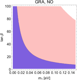
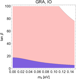
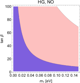
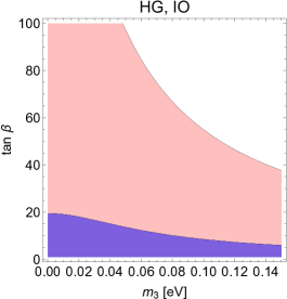
Figure 2: Allowed regions for $\tan\beta$ and $m_{\text{lightest}}$ for the NO and IO spectra in the cases of minimal (blue) and maximal (pink) corrections for $\cos\delta$ in the GRA mixing scheme (upper plots) and the HG mixing scheme (lower plots). We used the best fit values for the mixing angles. The high-energy scale is set to $10^{13}$ GeV.

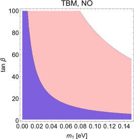
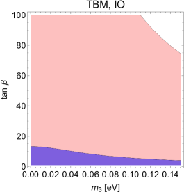
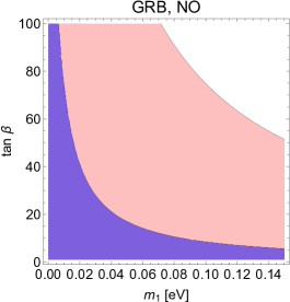
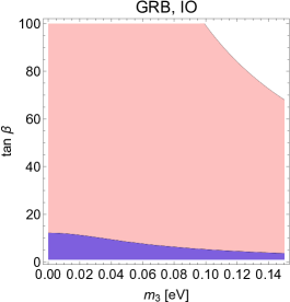
Figure 3: Allowed regions for $\tan\beta$ and $m_{\text{lightest}}$ for the NO and IO spectra in the cases of minimal (blue) and maximal (pink) corrections for $\cos\delta$ in the TBM mixing scheme (upper plots) and the GRB mixing scheme (lower plots). We used the best fit values for the mixing angles. The high-energy scale is set to $10^{13}$ GeV.

The allowed parameter regions in the $m_{\text{lightest}}$-$\tan\beta$ plane for the GRA and HG cases are shown in Fig. 2. For minimal corrections the parameter regions get severely constrained, $\tan\beta>20$ is incompatible with $\cos\delta(M_{S})\in[-1,1]$ for IO spectrum; for NO spectrum it is incompatible with $\cos\delta(M_{S})\in[-1,1]$ for $m_{1}\ \raisebox{-1.72218pt}{\hbox to0.0pt{$\sim$\hss}}\raisebox{1.72218pt}{$>$}\ 0.06$ eV. This can be understood since $\cos\delta(M_{Z})$ is positive for GRA mixing and the dominant contribution to $\delta(\cos\delta)$ comes from the correction due to $\delta\theta_{12}$, which is negative. A similar argument holds also for HG mixing.

For TBM and GRB $\cos\delta(M_{Z})$ is negative and the corrections further decrease the value. The plots for the allowed parameter regions can be found in Fig. 3.

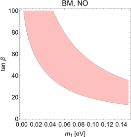
Figure 4: Allowed regions for $\tan\beta$ and $m_{\text{lightest}}$ for the NO and IO spectra in the case of maximal corrections for $\cos\delta$ in the BM mixing scheme. We used the best fit values of the mixing angles. For the minimal corrections there is no allowed parameter region which is compatible with $|\cos\delta|\leq 1$. We set the high-energy scale to $10^{13}$ GeV.

For BM mixing $\cos\delta(M_{Z})<-1$ for the best fit values of the angles, which is ruled out. As best approximation for the value of $\delta$ in the $\beta$-functions we use then $\delta(M_{Z})=\pi$. The dominant contribution to the correction is due to $\delta\theta_{13}$, which is positive for the maximal correction. Since $f_{13}$ is also positive in BM mixing, the value of $\cos\delta(M_{S})$ increases. Hence, the RG corrections have shifted $\cos\delta(M_{S})$ to allowed values, but for too large values of $\tan\beta$ the corrections overshoot $\cos\delta(M_{S})=1$ and the points are excluded. The allowed banana-shaped parameter regions are displayed in Fig. 4.

Note that in this example we have only employed the constraint on $\delta$ from eq. (2.9) at the high-energy scale. This corresponds to the scheme where $\theta_{23}^{e}\neq 0$. To fulfil the sum rule, $\theta_{12}$ is allowed to run weakly. In the case of the SM running, the RG effects are already small. In the case of the MSSM running, they are relatively small if the Majorana phases satisfy the relation $\alpha_{2}\approx\alpha_{1}+\pi$. The restrictions on the Majorana phases in the case of $\theta_{23}^{e}=0$ from eq. (2.7) are rather weak.

3.3 Implications of $\boldsymbol{\alpha_{2}-\alpha_{1}=0}$ and $\boldsymbol{\pi}$ and Small $\boldsymbol{\tan\beta}$

In this subsection we show how the specific values of the difference of the Majorana phases, namely, $\alpha_{2}-\alpha_{1}=0$ and $\pi$, contribute to the total likelihood profile obtained after the RG corrections are taken into account. These values might seem to be very special at a first glance but in fact many symmetric matrices belong at leading order to one of the two cases. The CP-violating effects of the requisite corrections from $\tilde{U}_{e}$ then might be controlled using, for instance, spontaneous CP violation with the discrete vacuum alignment method proposed in [41].

These two cases are also interesting because they correspond to extremal values of the neutrinoless double beta decay observable – the effective Majorana mass, $|m_{ee}|$, in the cases of neutrino mass spectrum with IO or of quasi-degenerate type (see, e.g., [5, 42]). For $\alpha_{2}-\alpha_{1}=0$, $|m_{ee}|$ is maximal in the two cases, while if $\alpha_{2}-\alpha_{1}=\pi$, $|m_{ee}|$ has a minimal value for both types of spectrum. In the case of IO spectrum and $m_{3}\ll m_{1,2}$, for example, $|m_{ee}|\cong\sqrt{\Delta m^{2}_{23}+m^{2}_{3}}\cos^{2}\theta_{13}\cong 4.7\times 10^{-2}$ eV if $\alpha_{2}-\alpha_{1}=0$, while for $\alpha_{2}-\alpha_{1}=\pi$ we have $|m_{ee}|\cong\sqrt{\Delta m^{2}_{23}+m^{2}_{3}}\cos^{2}\theta_{13}\cos 2\theta_{12}\ \raisebox{-1.72218pt}{\hbox to0.0pt{$\sim$\hss}}\raisebox{1.72218pt}{$>$}\ 0.014$ eV, where we have used the $3\sigma$ allowed ranges of $\Delta m^{2}_{23}$, $\sin^{2}\theta_{13}$ and $\sin^{2}\theta_{12}$ (for the IO spectrum) from Table 1.

As can be understood from eq. (3.1), in the case of equal Majorana phases, the running of $\theta_{12}$ is maximal, while for $\alpha_{2}-\alpha_{1}=\pi$ it is maximally suppressed. Since for the TBM, GRA, GRB and HG symmetry forms the correction to the tree-level value of $\cos\delta$ is dominated by the running of $\theta_{12}$ (see subsection 3.2), we consider as example the case of TBM and $\theta^{e}_{23}\neq 0$ with the values of $\alpha_{2}-\alpha_{1}$ specified above. The results we obtain in the GRA, GRB and HG cases are very similar.

It is interesting to see, in particular, what is the quantitative relation between the corrections obtained in the setup with relatively large $\tan\beta$, e.g., $\tan\beta=30$, and suppression of $\theta_{12}$ running due to $\alpha_{2}-\alpha_{1}=\pi$, and the setup with relatively small $\tan\beta$, e.g., $\tan\beta=5$ or $10$, but enhancement due to $\alpha_{2}=\alpha_{1}$.

To answer this question, we employ a simplified one-step integration procedure (linearised running), in which the high-energy values of the mixing parameters entering the sum rule are obtained using one-step integration of the exact one-loop beta functions for the mixing parameters from [20]. We set $\theta_{13}$, $\theta_{23}$, $\Delta m_{21}^{2}$, $\Delta m_{31(23)}^{2}$ to their best fit values and impose i) $\alpha_{2}=\alpha_{1}$, and ii) $\alpha_{2}=\alpha_{1}+\pi$. For each set of these low-energy values, we solve the high-energy sum rule for the low-energy value of $\theta_{12}$.

In order to perform a statistical analysis of the low-energy data after RG corrections we construct the $\chi^{2}$ function as

$$\chi^{2}(\vec{x})=\sum_{i=1}^{6}\chi^{2}_{i}(x_{i})\,,$$ (3.6)

where $\vec{x}=(\sin^{2}\theta_{12},\sin^{2}\theta_{13},\sin^{2}\theta_{23},\delta,\Delta m_{21}^{2},\Delta m_{31(23)}^{2})$ for the NO (IO) spectrum, and $\chi^{2}_{i}$ are one-dimensional projections taken from [7]. In order to obtain the one-dimensional projection $\chi^{2}(\delta)$ from the constructed $\chi^{2}(\vec{x})$ function we need to minimise the latter with respect to all other parameters ($\sin^{2}\theta_{ij}$, $\Delta m_{21}^{2}$ and $\Delta m_{31(23)}^{2}$), i.e., we need to find a minimum of $\chi^{2}(\vec{x})$ for a fixed value of $\delta$:

$$\chi^{2}(\delta)=\min\left[\chi^{2}(\vec{x})|_{\delta={\rm const}}\right]\,.$$ (3.7)

The likelihood function $L$, which represents the most probable values of $\delta$ in each of the considered cases, reads

$$L(\delta)=\exp\left(-\frac{\chi^{2}(\delta)}{2}\right)\,.$$ (3.8)

We will present the results in terms of the likelihood functions, considering three values for the absolute mass scale, $m_{\text{lightest}}=0.005$, $0.01$ and $0.05$ eV, and four values of $\tan\beta=5$, $10$, $30$ and $50$.

It is worth noting here that, as shown in ref. [20] (see eq. (26) therein), for the running of the difference $\alpha_{1}-\alpha_{2}$ we have up to $\mathcal{O}(\theta_{13})$ terms:

$$\frac{\text{d}}{\text{d}\,\ln(\mu/\mu_{0})}(\alpha_{1}-\alpha_{2})\propto\sin(\alpha_{1}-\alpha_{2})\,.$$ (3.9)

This implies that if the phases are equal (different by $\pi$) at some scale to a good approximation, they remain equal (differ by $\pi$) at another scale. Thus, the relation imposed by us at the low scale holds also at the high scale (up to $\mathcal{O}(\theta_{13})$ corrections).

Figure 5: Likelihood function vs. $\delta$ in the case of non-zero $\theta^{e}_{23}$ for the TBM symmetry form of the matrix $\tilde{U}_{\nu}$ and the NO spectrum. The dotted black line stands for likelihood extracted from the global analysis in [7]. The blue, orange, green and red lines are for the running within MSSM with $\tan\beta=5$, $10$, $30$ and $50$, respectively. The left panels correspond to $\alpha_{2}=\alpha_{1}$, while the right panels are for $\alpha_{2}=\alpha_{1}+\pi$.

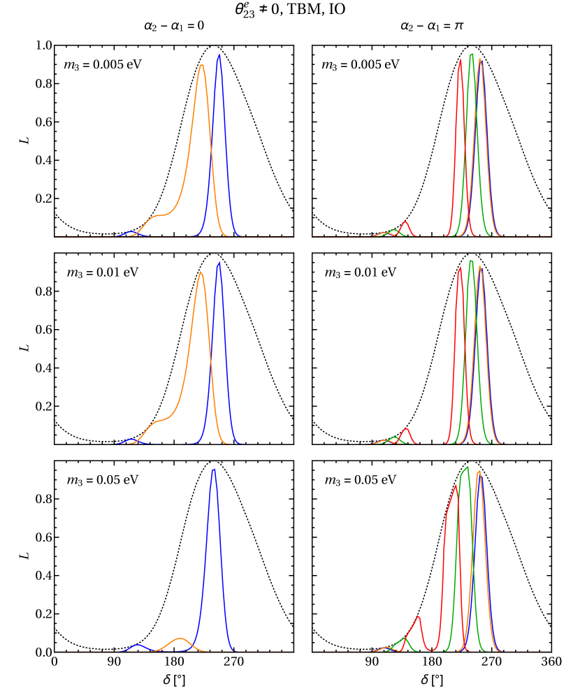
Figure 6: Likelihood function vs. $\delta$ in the case of non-zero $\theta^{e}_{23}$ for the TBM symmetry form of the matrix $\tilde{U}_{\nu}$ and the IO spectrum. The dotted black line stands for likelihood extracted from the global analysis in [7]. The blue, orange, green and red lines are for the running within MSSM with $\tan\beta=5$, $10$, $30$ and $50$, respectively. The left panels correspond to $\alpha_{2}=\alpha_{1}$, while the right panels are for $\alpha_{2}=\alpha_{1}+\pi$.

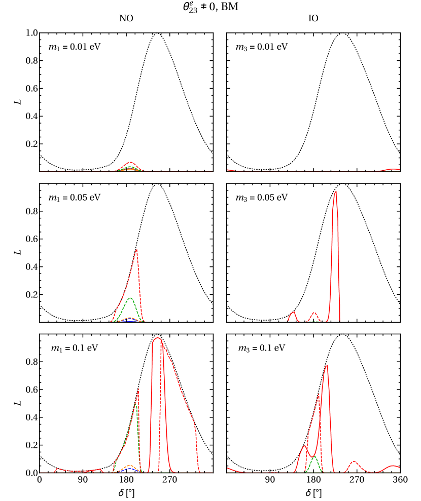
Figure 7: Likelihood function vs. $\delta$ in the case of non-zero $\theta^{e}_{23}$ for the BM symmetry form of the matrix $\tilde{U}_{\nu}$. The dotted black line stands for likelihood extracted from the global analysis in [7]. The blue, orange, green and red lines are for the running within MSSM with $\tan\beta=5$, $10$, $30$ and $50$, respectively. The solid lines correspond to $\alpha_{2}=\alpha_{1}$. The dashed lines correspond to $\alpha_{2}=\alpha_{1}+\pi$. Note that the lines for $\tan\beta<50$ are often barely visible.

We present graphically the results obtained for the TBM symmetry form in Figs. 5 and 6 for the NO and IO neutrino mass spectra, respectively. The dotted black line stands for likelihood extracted from the global analysis [7]. The blue, orange, green and red lines are for $\tan\beta=5$, $10$, $30$ and $50$, respectively. The left panels in each of the two figures correspond to $\alpha_{2}=\alpha_{1}$, while the right panels are for $\alpha_{2}=\alpha_{1}+\pi$.

Several comments are in order. As expected, the results for $\alpha_{2}-\alpha_{1}=\pi$ and small $\tan\beta$, $\tan\beta=5$ and $10$ (blue and orange lines, respectively), are quantitatively very similar to the result without running (this is why we do not present the latter in the plots) for all three mass scales considered and both orderings due to the suppression of the running of $\theta_{12}$ discussed above. However, this is not the case for the large values of $\tan\beta=30$ and $50$ (green and red lines, respectively) and the NO spectrum with $m_{1}=0.05$ eV, and for all three values of $m_{3}$ considered in the case of the IO spectrum. Clearly, the enhancement due to $\tan\beta$ prevails over the suppression due to the Majorana phases in these cases.

The next interesting point to note is that for the IO spectrum, the corrections in the case of $\tan\beta=5$ and $\alpha_{2}=\alpha_{1}$ (blue line) are comparable with the corrections for $\tan\beta=30$ and $\alpha_{2}=\alpha_{1}+\pi$ (green line) for all three mass scales considered. A similar observation holds also for the NO spectrum if $m_{1}=0.05$ eV: the corrections for $\tan\beta=10$ and $\alpha_{2}=\alpha_{1}$ (orange line) are similar in magnitude to those for $\tan\beta=30$ and $\alpha_{2}-\alpha_{1}=\pi$ (green line).

Further, we note also that the absence of the green and red lines, corresponding to $\tan\beta=30$ and $50$ and equal Majorana phases, in all cases, except for NO with $m_{1}=0.005$ eV and $m_{1}=0.01$ eV, reflects the fact that the RG corrections lead, in particular, to a low-energy value of $\theta_{12}$, which is outside of the current $3\sigma$ range. For the IO spectrum with $m_{3}=0.05$ eV and $\alpha_{2}=\alpha_{1}$, even for $\tan\beta=10$ (orange line) the RG corrections are quite large, such that only a small region of values of $\delta$ around $\pi$ is allowed, with the likelihood of these values being suppressed.

For the BM symmetry form the results we obtain are quite different. In this case we consider values of $m_{\text{lightest}}=0.01$, $0.05$ and $0.1$ eV, and $\tan\beta=5$, $10$, $30$ and $50$. We find that the small values of $\tan\beta$ considered, $\tan\beta=5$, 10, cannot provide the RG corrections which allow one to have $\cos\delta\in[-1,1]$ and low-energy values of the mixing angles compatible with the current data (except for the small range of values of $\delta$ close to $\pi$ allowed without running). For the large values of $\tan\beta$ and the NO spectrum, we get significant RG corrections compatible with all constraints, as can be seen from Fig. 7, i) for $\alpha_{2}-\alpha_{1}=\pi$ (dashed lines), provided $m_{1}\ \raisebox{-1.72218pt}{\hbox to0.0pt{$\sim$\hss}}\raisebox{1.72218pt}{$>$}\ 0.05$ eV, and ii) for $\alpha_{2}=\alpha_{1}$ (solid line) if $m_{1}\cong 0.10$ eV and $\tan\beta=50$. For the IO spectrum and $m_{3}\ \raisebox{-1.72218pt}{\hbox to0.0pt{$\sim$\hss}}\raisebox{1.72218pt}{$>$}\ 0.05$ eV, the predictions are compatible with the data for $\alpha_{2}=\alpha_{1}$ provided $\tan\beta=50$. If $m_{3}=0.1$ eV, $\alpha_{2}-\alpha_{1}=\pi$ also contributes to the final likelihood profile for $\tan\beta=50$, although this contribution is less favoured.

As already discussed above, the running of $\theta_{12}$ is suppressed if the difference of the Majorana phases is equal to $\pi$, otherwise the running of $\theta_{12}$ is always the dominant correction to $\cos\delta$. If the running of $\theta_{12}$ is minimal, the running of $\theta_{23}$ and $\theta_{13}$ is dominant (for a maximal running of $\theta_{13}$ we need additionally to have $\delta=\alpha_{2}$). Then $\delta\theta_{13}$ and $\delta\theta_{23}$ are roughly two orders of magnitude larger then $\delta\theta_{12}$. This implies that the correction to $\cos\delta$ in the HG, GRA, GRB and TBM mixing schemes is not longer determined by the running of $\theta_{12}$ but by the running of $\theta_{23}$ and $\theta_{13}$. For BM mixing the contribution of $\delta\theta_{13}$ is still dominant. The sign and size of the correction to $\cos\delta$ depends on $\delta$ because the size of $\delta\theta_{13}$ depends on $\delta$ and the contributions to $\delta(\cos\delta)$ by the running of $\theta_{23}$ and $\theta_{13}$ are approximately equal.

Finally, we would like to note that the cases studied in the present subsection were analysed rather qualitatively in [27], considering only the running of $\theta_{12}$. Our analysis goes beyond the discussion in [27], since we present explicitly in graphic form the impact of the RG effects on the likelihood functions (Figs. 5 – 7). In particular, as was discussed above, the results depend strongly on the symmetry form considered – the TBM, GRA, GRB and HG forms on the one hand and the BM form on the other – and this distinction was not discussed in [27]. Furthermore, in our quantitative results we find a region of parameter space where their conclusions are not fully correct. Although this region seems somewhat tuned, it is actually motivated, as we mentioned above, in setups with spontaneous CP violation. We find that, e.g., in the case of the TBM symmetry form, for $m_{3}=0.01$ eV (IO), $\tan\beta=30$ and $\alpha_{2}-\alpha_{1}=\pi$ (green line in the corresponding panel of Fig. 6) the RG corrections are noticeable, in contrast to the conclusion in [27] that the RG corrections can be neglected for $\tan\beta\ \raisebox{-1.72218pt}{\hbox to0.0pt{$\sim$\hss}}\raisebox{1.72218pt}{$<$}\ 35$ if the spectrum is not quasi-degenerate.

3.4 Notes on the $\boldsymbol{\theta_{23}^{e}=0}$ Case

Before we turn to the numerical results we want to make a few more remarks on the case of $\theta_{23}^{e}=0$, i.e., imposing also the sum rule from eq. (2.7) at the high scale. This will help to understand the numerical results in the next section. In eq. (2.10) we can replace $\theta_{12}(M_{S})$ by $\theta_{12}(M_{Z})$ plus the small RG correction $\delta\theta_{12}$ in which we expand. Since $\theta_{13}$ and $\delta\theta_{13}$ are small we can neglect the latter ($\theta_{13}(M_{S})\approx\theta_{13}(M_{Z})$) and expand the correction in the first to end up with

$$\cos\delta(M_{S})\approx\cos\delta(M_{Z})+\frac{1-\cos 2\theta_{12}\,\cos 2\theta_{12}^{\nu}}{\theta_{13}\sin^{2}2\theta_{12}}\delta\theta_{12}~{}.$$ (3.10)

In the case of BM mixing $\cos\delta(M_{Z})$ is smaller than $-1$ for the best fit values of the angles and the correction is always negative since the running of $\theta_{12}$ has a fixed sign. Note, that the value of $\cos\delta(M_{Z})$ could be adjusted by $\theta_{23}^{e}\neq 0$ to a value larger than $-1$, cf. eq. (2.9). So, from that estimate we expect the BM mixing scheme not to be valid in the case of $\theta_{23}^{e}=0$. This is confirmed in our extensive numerical scan, where we employed the exact sum rules from eqs. (2.7, 2.10) and the full 1-loop $\beta$-functions for all parameters but did not find any physically acceptable points as well. Nevertheless, our estimate is a bit rough and a numerical scan cannot cover the whole parameter space such that a tiny, highly tuned region of parameter space might still be allowed.

Let us now turn to the other mixing cases. There the absolute value of $\cos\delta(M_{Z})$ in our estimate eq. (3.10) is always smaller than one. For TBM and GRB it is still negative, but for TBM mixing, for instance, we get

$$\cos\delta(M_{Z})\approx-0.21\;,$$ (3.11)

which allows for a sizeable correction of $\theta_{12}$ up to $-6.5^{\circ}$, so that these two scenarios are not disfavoured by our estimate. For GRA and HG mixing the first term is even positive such that we can account for even more sizeable RG corrections in these cases.

4 Numerical Results

In the present section we will first describe our numerical approach before we show the results we obtain for the $\delta$ likelihood functions in the TBM, GRA, GRB, BM and HG mixing schemes in the cases of $\theta_{23}^{e}\neq 0$ and $\theta_{23}^{e}=0$.

4.1 Numerical Approach

To obtain the low-energy predictions for $\delta$ from the high-scale mixing sum rule, eq. (2.9) in the case of $\theta^{e}_{23}\neq 0$ (eq. (2.10) in the case of $\theta^{e}_{23}=0$), we employ the running of the parameters using the REAP package [40]. For the running we set the low-energy scale to be $M_{Z}$ and the high-energy scale to be equal to the seesaw scale $M_{S}\approx 10^{13}$ GeV. Since the dependence on the scales is only logarithmic a mild change of the high-energy or low-energy scale would not change our results significantly.

In our scans we present the results for the SM and MSSM extended minimally by the Weinberg operator. We have fixed the scale where we switch from the SM to MSSM RGEs to 1 TeV. Again the dependence on the scale is only logarithmic and hence weak. The exact supersymmetric (SUSY) particle spectrum plays only a minor role since we have neglected the SUSY threshold corrections [43].

In the MSSM we consider as benchmarks $\tan\beta=30$ and $\tan\beta=50$. In the SM the running is relatively small and hence the results are very similar to the results without running. In fact the SM results look like the results obtained in [13] apart from relatively small changes due to the different global fit results [8] used therein. For a given mass scale and a given model (SM or MSSM with a given $\tan\beta$), we employ the mixing sum rules at the high scale to determine $\delta$ (and $\theta_{23}$ for $\theta_{23}^{e}=0$) at the low scale depending on the other parameters. For a given mass scale and a given model (SM or MSSM with a given $\tan\beta$), we determine the low-scale parameters (the angles, mass squared differences and the Majorana phases) such that the mixing sum rule eq. (2.9) (and eq. (2.10) for $\theta_{23}^{e}=0$) at the high scale is fulfilled and their likelihood function is maximal. We choose a “small” neutrino mass scale, $m_{\text{lightest}}=0.01$ eV, a “medium” mass scale, $m_{\text{lightest}}=0.05$ eV, and a “large” mass scale, $m_{\text{lightest}}=0.1$ eV. The “large” neutrino mass scale is still compatible with the cosmological bound on the sum of the neutrino masses [44]

$$\sum m_{\nu}<0.49\text{ eV.}$$ (4.1)

Note that for very small neutrino mass scales, $m_{\text{lightest}}\ll 0.01$ eV and sufficiently small $\tan\beta$, the RG effects are negligibly small even in the MSSM. We present the results for different cases considered in the present study in terms of the likelihood functions defined in eq. (3.8).

4.2 Results for Different Mixing Schemes in the Case of Non-zero $\boldsymbol{\theta^{e}_{23}}$

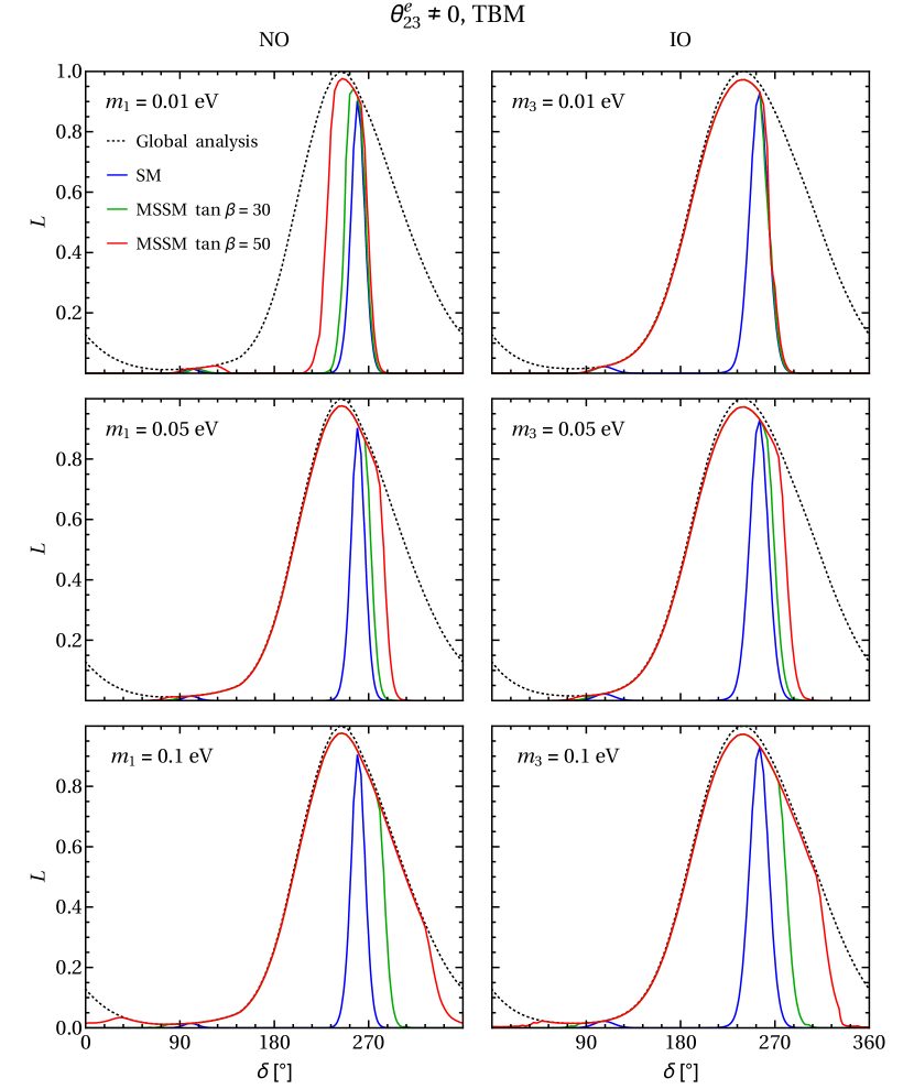
Figure 8: Likelihood function vs. $\delta$ in the case of non-zero $\theta^{e}_{23}$ for the TBM symmetry form of the matrix $\tilde{U}_{\nu}$ in all the setups considered. The dotted line stands for likelihood extracted from the global analysis in [7]. The blue line is for the SM running, while the green and red lines are for the running within MSSM with $\tan\beta=30$ and $\tan\beta=50$, respectively.

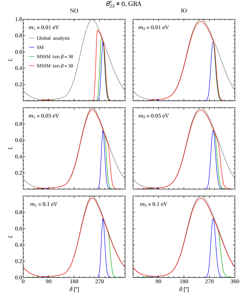
Figure 9: Likelihood function vs. $\delta$ in the case of non-zero $\theta^{e}_{23}$ for the GRA symmetry form of the matrix $\tilde{U}_{\nu}$ in all the setups considered. The dotted line stands for likelihood extracted from the global analysis in [7]. The blue line is for the SM running; the green and red lines are for the running within MSSM with $\tan\beta=30$ and $\tan\beta=50$, respectively.

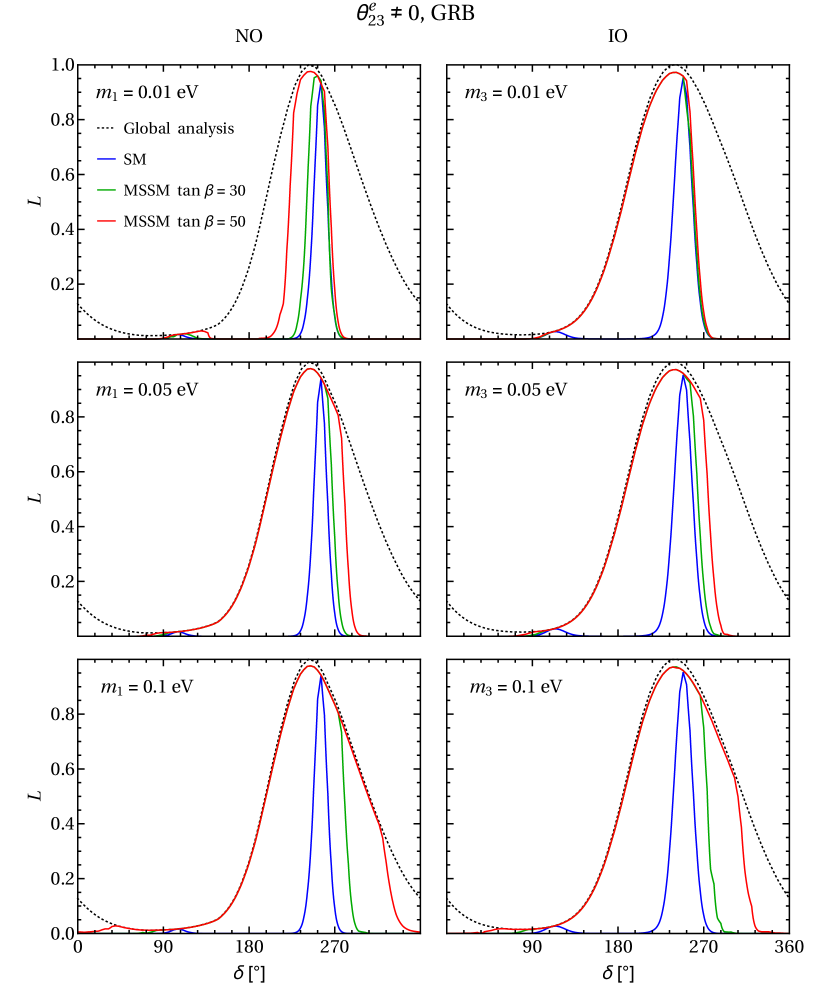
Figure 10: Likelihood function vs. $\delta$ in the case of non-zero $\theta^{e}_{23}$ for the GRB symmetry form of the matrix $\tilde{U}_{\nu}$ in all the setups considered. The dotted line stands for likelihood extracted from the global analysis in [7]. The blue line is for the SM running, while the green and red lines are for the running within MSSM with $\tan\beta=30$ and $\tan\beta=50$, respectively.

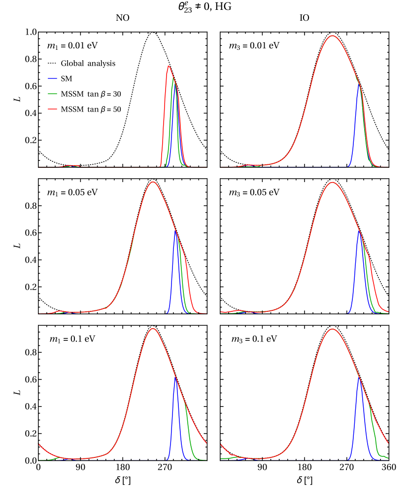
Figure 11: Likelihood function vs. $\delta$ in the case of non-zero $\theta^{e}_{23}$ for the HG symmetry form of the matrix $\tilde{U}_{\nu}$ in all the setups considered. The dotted line stands for likelihood extracted from the global analysis in [7]. The blue line is for the SM running; the green and red lines are for the running within MSSM with $\tan\beta=30$ and $\tan\beta=50$, respectively.

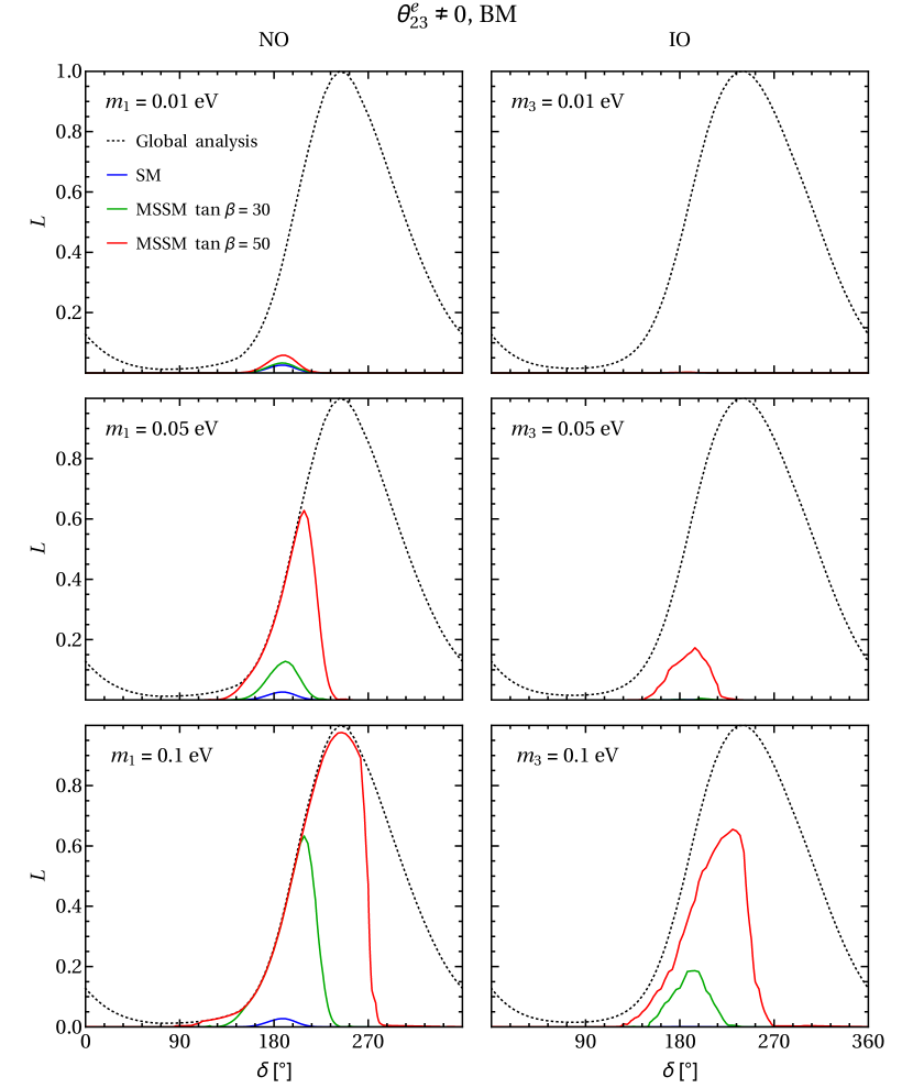
Figure 12: Likelihood function vs. $\delta$ in the case of non-zero $\theta^{e}_{23}$ for the BM symmetry form of the matrix $\tilde{U}_{\nu}$ in all the setups considered. The dotted line stands for likelihood extracted from the global analysis in [7]. The blue line is for the SM running, while the green and red lines are for the running within MSSM with $\tan\beta=30$ and $\tan\beta=50$, respectively.

We begin our discussion of the numerical results with the case of non-zero $\theta^{e}_{23}$. In Figs. 8 – 11 we show the likelihood functions versus $\delta$ for the TBM, GRA, GRB and HG symmetry forms of the matrix $\tilde{U}_{\nu}$ in all setups. The blue line in these figures represents the SM running result, the green and red lines are for the MSSM running with $\tan\beta=30$ and $\tan\beta=50$, respectively. The SM line practically coincides with the line corresponding to the result without running, as expected. For this reason we do not show the latter in the plots. The dotted black line stands for the likelihood extracted from the global analysis [7] which corresponds to the likelihood for $\delta$ without imposing any sum rule. We note that the whole procedure is numerically very demanding and hence there are some tiny wiggles in the likelihoods which do not have any physical meaning. Note also that the mixing sum rule has two solutions but the solution $\delta\approx 90^{\circ}$ has a small likelihood and is therefore barely visible in the plots.

As we have already indicated, the SM results are very similar to the results obtained in [13] without running. This implies that, as was concluded in [13] (see also [12]), using the data on neutrino mixing angles and a sufficiently precise measurement of $\cos\delta$ it will be possible to distinguish between the three groups of schemes: the TBM and GRB group, the GRA and HG group, and the BM scheme. Distinguishing between the GRA and HG schemes is experimentally very demanding, but not impossible, while distinguishing between the TBM and GRB seems practically extremely difficult (if not impossible) to achieve (see [13, 14] for further details).

In the MSSM, the results depend on the value of the lightest neutrino mass, the type of spectrum – NO or IO – the neutrino masses obey, on the value of $\tan\beta$ as well as on the uncertainties in the measured values of the neutrino oscillation parameters. As expected, for increasing $\tan\beta$ and increasing absolute neutrino mass scale, the difference with the predictions without running increases. The allowed regions for $\delta$ start to broaden and, e.g., for the largest value of $\tan\beta=50$ and $m_{1}=0.05$ eV and 0.10 eV ($m_{3}=0.01$ eV, 0.05 eV and 0.10 eV) in the case of NO (IO) spectrum, the likelihood profile in the cases of the TBM, GRA, GRB and HG mixing schemes practically coincides with the likelihood for $\delta$ obtained without imposing the sum rule constraint, the difference between the two profiles being noticeable only for values of $\delta$ lying approximately in the interval $\delta\sim(270^{\circ}-360^{\circ})$. As already discussed in the previous section, the running of $\cos\delta$ in the TBM, GRA, GRB and HG mixing schemes is mainly influenced by the running of $\theta_{12}$ which has a fixed negative sign and hence has a tendency to shift $\delta$ to values smaller than $270^{\circ}$. For NO spectrum, $m_{1}\leq 0.01$ eV and $\tan\beta=30$, a measured value of $\delta\ \raisebox{-1.72218pt}{\hbox to0.0pt{$\sim$\hss}}\raisebox{1.72218pt}{$<$}\ 260^{\circ}$ would favour the TBM and GRB schemes. For $m_{1}=0.05$ eV (or $m_{1}=0.01$ eV) and the same value of $\tan\beta=30$, a measurement of $\delta\ \raisebox{-1.72218pt}{\hbox to0.0pt{$\sim$\hss}}\raisebox{1.72218pt}{$>$}\ 290^{\circ}$ would make the GRA and HG schemes more probable. For $\tan\beta=50$, $m_{1}=0.05$ eV (or $m_{1}=0.10$ eV), and given the current uncertainties in the measured values of the neutrino oscillation parameters, the TBM, GRA, GRB and HG schemes lead to very similar predictions for $\delta$.

For the IO spectrum the RG effects are larger and therefore the broadening happens in the four schemes under discussion – TBM, GRA, GRB and HG – already for the “small” neutrino mass scale. Since the likelihood profiles are so broad and nearly identical even for the “small” and “medium” mass scales, except for certain differences in the interval $\delta\cong(270^{\circ}-360^{\circ})$, and given the current uncertainties in the measured values of the neutrino oscillation parameters, it will be difficult in the MSSM with $\tan\beta\ \raisebox{-1.72218pt}{\hbox to0.0pt{$\sim$\hss}}\raisebox{1.72218pt}{$>$}\ 30$ to distinguish between any of the four schemes considered using only a determination of $\delta$.

For the BM mixing scheme the results are very different. This scheme is strongly disfavoured for the currently allowed ranges of the mixing parameters without considering RG effects. Therefore, the maximal value of the likelihood in the SM running case is relatively small. In the MSSM the running increases the value of $\cos\delta$ to physical values, as explained in the previous section. In addition both the maximal value of the likelihood function increases and the position of the likelihood maximum shifts from $\delta\cong 180^{\circ}$ towards $\delta=270^{\circ}$ (see Fig. 12). Again the likelihood profile broadens with increasing of the absolute neutrino mass scale and $\tan\beta$ and at $\delta\ \raisebox{-1.72218pt}{\hbox to0.0pt{$\sim$\hss}}\raisebox{1.72218pt}{$<$}\ 270^{\circ}$ for NO spectrum tends to approach the likelihood function for $\delta$ obtained without imposing the sum rule. In the case of IO spectrum, the BM scheme is strongly disfavoured for $m_{3}\ \raisebox{-1.72218pt}{\hbox to0.0pt{$\sim$\hss}}\raisebox{1.72218pt}{$<$}\ 0.05$ eV even for $\tan\beta=50$.

4.3 Results for Different Mixing Schemes in the Case of Zero $\boldsymbol{\theta^{e}_{23}}$

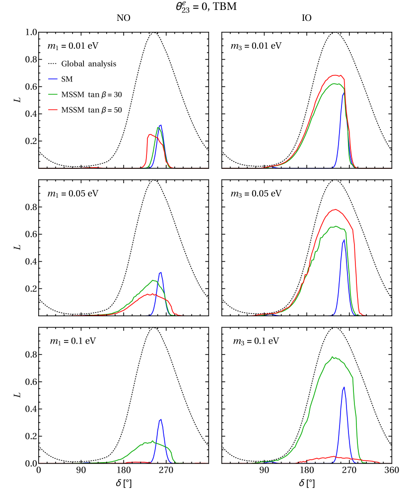
Figure 13: Likelihood function vs. $\delta$ in the case of zero $\theta^{e}_{23}$ for the TBM symmetry form of the matrix $\tilde{U}_{\nu}$ in all the setups considered. The dotted line stands for likelihood extracted from the global analysis in [7]. The blue line is for the SM running. Finally, the green and red lines are for the running within MSSM with $\tan\beta=30$ and $\tan\beta=50$, respectively.

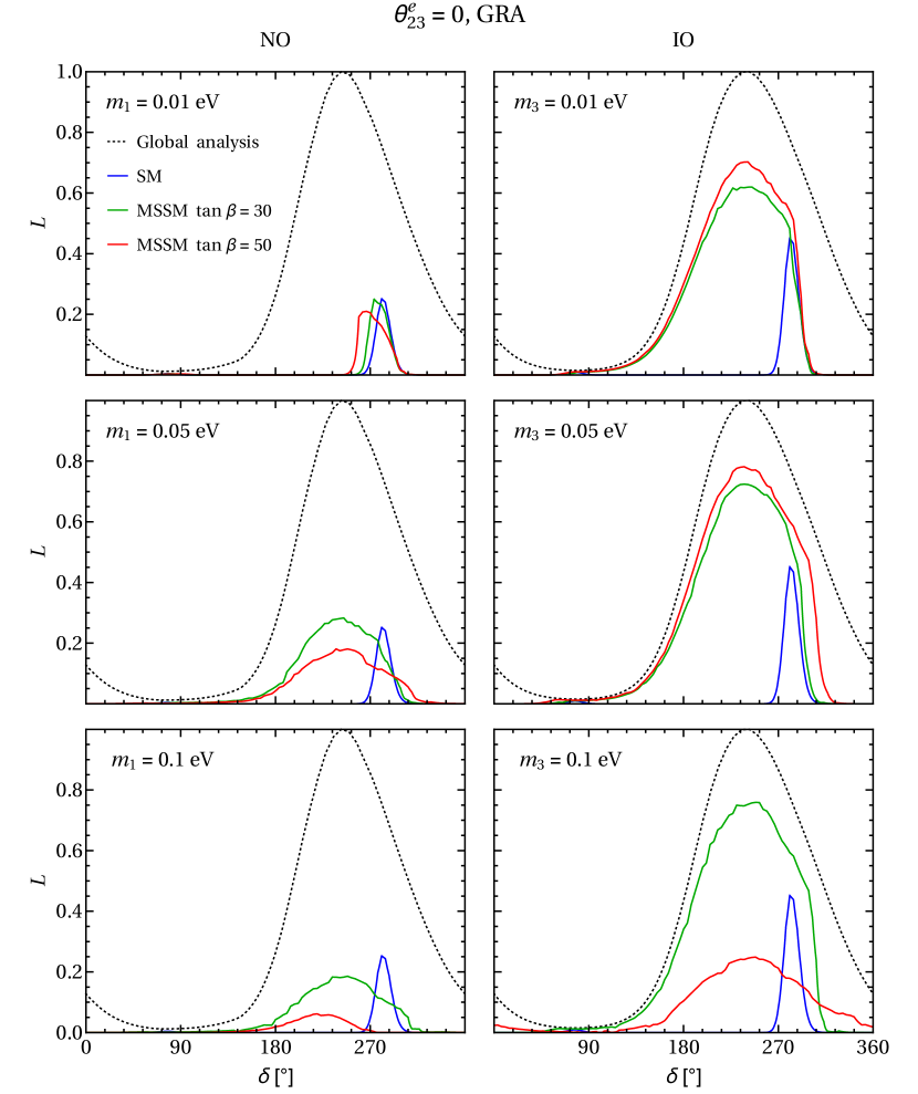
Figure 14: Likelihood function vs. $\delta$ in the case of zero $\theta^{e}_{23}$ for the GRA symmetry form of the matrix $\tilde{U}_{\nu}$ in all the setups considered. The dotted line stands for likelihood extracted from the global analysis in [7]. The blue line is for the SM running. Finally, the green and red lines are for the running within MSSM with $\tan\beta=30$ and $\tan\beta=50$, respectively.

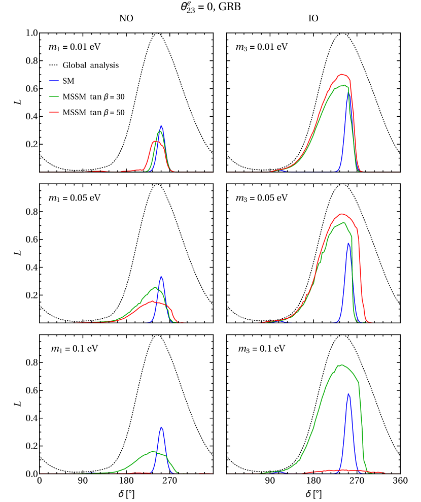
Figure 15: Likelihood function vs. $\delta$ in the case of zero $\theta^{e}_{23}$ for the GRB symmetry form of the matrix $\tilde{U}_{\nu}$ in all the setups considered. The dotted line stands for likelihood extracted from the global analysis in [7]. The blue line is for the SM running. Finally, the green and red lines are for the running within MSSM with $\tan\beta=30$ and $\tan\beta=50$, respectively.

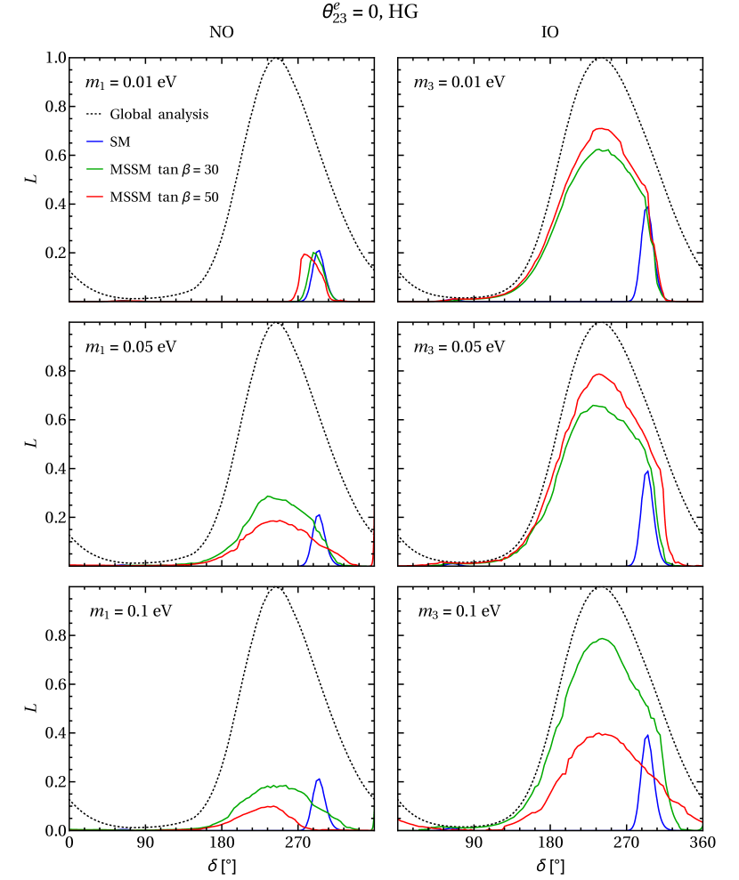
Figure 16: Likelihood function vs. $\delta$ in the case of zero $\theta^{e}_{23}$ for the HG symmetry form of the matrix $\tilde{U}_{\nu}$ in all the setups considered. The dotted line stands for likelihood extracted from the global analysis in [7]. The blue line is for the SM running. Finally, the green and red lines are for the running within MSSM with $\tan\beta=30$ and $\tan\beta=50$, respectively.

In Figs. 13 – 16 we present the results in the case of $\theta^{e}_{23}=0$. Again, the blue line in these figures represents the SM running result, the green and red lines are for the MSSM running with $\tan\beta=30$ and $\tan\beta=50$, respectively. The dotted black line stands for the likelihood extracted from the global analysis [7] which corresponds to the likelihood for $\delta$ without imposing any sum rule. Similar to the case of non-zero $\theta_{23}^{e}$, the SM line practically coincides with the line corresponding to the result without running, as expected. Therefore we do not show the latter in the plots. Note again that the small wiggles in the likelihoods are of numerical origin and not physical.

For the TBM, GRA, GRB and HG mixing schemes we observe similar to the case of non-zero $\theta_{23}^{e}$ broadening of the likelihood with increasing $\tan\beta$ and increasing absolute neutrino mass scale. But in contrast to the case of $\theta^{e}_{23}\neq 0$, the likelihood does not reach the likelihood for $\delta$ without imposing the sum rule considered. The major difference with respect to the results obtained in the case of $\theta_{23}^{e}\neq 0$ is that due to the constraint on $\theta_{23}$ from eq. (2.7) at the high scale, the low-scale mixing parameters are more severely constrained and not necessarily close to their respective best fit values.

As Figs. 13 – 16 show, for the values of ${\rm min}(m_{j})$ and $\tan\beta$ considered, the NO spectrum is less favoured (i.e., has a smaller likelihood for any given $\delta$ and smaller maximum likelihood) than the IO spectrum. The sum rule, eq. (2.7), restricts $\theta_{23}$ to be slightly smaller than $45^{\circ}$ at the high scale. Since the running of this angle has a fixed negative sign for NO spectrum, its low-scale value is larger than its high scale value and pushed outside of the NO 1$\sigma$ region. On the other hand, for IO spectrum the low-scale value of $\theta_{23}$ is always smaller than $45^{\circ}$ due to the running and the sum rule. However, in this case there is a second 1$\sigma$ region below maximal mixing besides the region around the best fit value which is larger than $45^{\circ}$.

In the case of the TBM and GRB schemes, the case of ${\rm min}(m_{j})=0.10$ eV and $\tan\beta=50$ is strongly disfavoured for both NO and IO spectra, while for the GRA and HG schemes it is less favoured than the ${\rm min}(m_{j})=0.10$ eV and $\tan\beta=30$ case.

As explained in subsection 3.4, in order to satisfy the sum rule eq. (2.10) for zero $\theta_{23}^{e}$, $\theta_{12}$ is not allowed to run strongly. This leads to the relatively small likelihood for $\tan\beta=50$ and $m_{\text{lightest}}=0.1$ eV seen in Figs. 13 – 16. For TBM and GRB mixing the constraint on the running of $\theta_{12}$ is even more severe than for GRA and HG mixing and the likelihood in these schemes is hence even smaller for $\tan\beta=50$ and $m_{\text{lightest}}=0.1$ eV.

For BM mixing our analytical estimates have indicated that this scheme is not valid due to the severe constraint on the running of $\theta_{12}$. In our extensive numerical scans we did not find any valid, i.e., physically acceptable, parameter points as well.

5 Summary and Conclusions

We presented a systematic study of the effects of RG corrections on sum rules for the Dirac CPV phase, eqs. (2.9) and (2.10). These corrections are present in every high-energy model, when running down to the low scale where experiments take place. We answered the question how stable the predictions from the sum rules are in the cases of charged lepton corrections characterised by i) $\theta_{12}^{e}\neq 0,~{}\theta_{23}^{e}\neq 0,~{}\theta_{13}^{e}=0$ and ii) $\theta_{12}^{e}\neq 0,~{}\theta_{23}^{e}=0,~{}\theta_{13}^{e}=0$ to TBM, BM, GRA, GRB or HG mixing in the neutrino sector.

To this aim we first reviewed the framework in which we obtain the mixing sum rules. Then we presented analytical estimates of the allowed parameter space if we take RG corrections into account. These estimates were subsequently verified numerically. To obtain the numerical results for the allowed ranges of $\delta$ we used as three benchmark cases the SM running (where the running effects are small) and the MSSM running with $\tan\beta=30$ and $\tan\beta=50$ (where the running effects become larger with increasing $\tan\beta$). Furthermore, we considered three mass scales: a “small” mass scale ($m_{\text{lightest}}=0.01$ eV), a “medium” mass scale ($m_{\text{lightest}}=0.05$ eV) and a “large” mass scale ($m_{\text{lightest}}=0.1$ eV), where the RG effects increase with the mass scale. We presented the results in terms of the likelihood functions for each case (SM or MSSM with a given $\tan\beta$, and a given mass scale). Our numerical results are obtained using the current best fit values and uncertainties on the neutrino oscillation parameters derived in the global analysis of the neutrino oscillation data performed in [7].

Our results have shown that the RG effects can change significantly the allowed low-energy ranges for $\delta$, especially when we employ the MSSM running with the “medium” and “large” mass scales. In the case of $\theta^{e}_{23}\neq 0$ the allowed regions for $\delta$ broaden and the likelihood profiles approach the likelihood for $\delta$ extracted from the global analysis (without imposing the sum rules considered). For the TBM, GRA, GRB and HG symmetry forms we found the allowed ranges of values of $\delta$ to be shifted from values close to (somewhat larger than) $270^{\circ}$ to values somewhat smaller than (close to) $270^{\circ}$. For BM mixing, which is strongly disfavoured by the current data without taking into account the running of the neutrino parameters, we found that the RG corrections partially reconstitute compatibility of this symmetry form with the data. With the increasing of ${\rm min}(m_{j})$ and $\tan\beta$, the values of $\delta$ in this case shift from $\delta\sim 180^{\circ}$ towards $270^{\circ}$. In the case of $\theta^{e}_{23}=0$ and for the TBM, GRA, GRB and HG mixing schemes the likelihood profiles broaden with increasing $\tan\beta$ and increasing mass scale, similarly to the case of non-zero $\theta^{e}_{23}$. The main difference is that now they do not reach the likelihood for $\delta$ obtained without imposing the sum rule. The reason for that is the constraint on $\theta_{23}$ from eq. (2.7) at the high scale, due to which the low-scale mixing parameters are more severely constrained and not necessarily close to their respective best fit values. Finally, we found that in this case the RG corrections are not sufficient to restore even partial compatibility of BM mixing with the current data.

In conclusion, our results show that the RG effects on the mixing sum rules in SUSY models with ${\rm min}(m_{j})\ \raisebox{-1.72218pt}{\hbox to0.0pt{$\sim$\hss}}\raisebox{1.72218pt}{$>$}\ 0.01$ eV and $\tan\beta\ \raisebox{-1.72218pt}{\hbox to0.0pt{$\sim$\hss}}\raisebox{1.72218pt}{$>$}\ 30$ have to be taken into account to realistically probe the predictions from the sum rules in concrete models.

Appendix A Likelihood Functions for $\boldsymbol{\cos\delta}$

In the past there have been already extensive studies on the likelihoods for the Dirac CPV phase derived from mixing sum rules. In [13, 14, 15, 27], in particular, results for the TBM, GRA, GRB, HG and BM mixing schemes were presented neglecting the RG corrections. However, in the indicated publications the likelihoods for $\cos\delta$ and not for $\delta$ have been derived. For better comparison with these results we include in the present Appendix Figs. 17 – 21 (Figs. 22 – 25) with the likelihood functions for $\cos\delta$ in the case of $\theta^{e}_{23}\neq 0$ ($\theta^{e}_{23}=0)$.

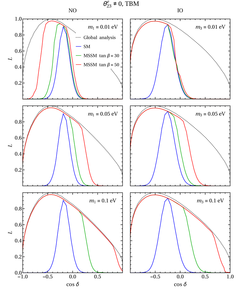
Figure 17: Likelihood function vs. $\cos\delta$ in the case of non-zero $\theta^{e}_{23}$ for the TBM symmetry form of the matrix $\tilde{U}_{\nu}$ in all the setups considered. The dotted line stands for likelihood extracted from the global analysis in [7]. The blue line is for the SM running. Finally, the green and red lines are for the running within MSSM with $\tan\beta=30$ and $\tan\beta=50$, respectively.

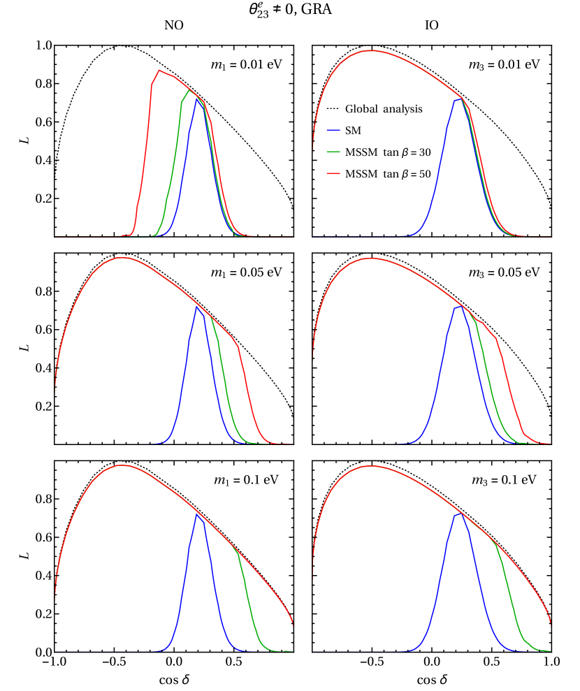
Figure 18: Likelihood function vs. $\cos\delta$ in the case of non-zero $\theta^{e}_{23}$ for the GRA symmetry form of the matrix $\tilde{U}_{\nu}$ in all the setups considered. The dotted line stands for likelihood extracted from the global analysis in [7]. The blue line is for the SM running. Finally, the green and red lines are for the running within MSSM with $\tan\beta=30$ and $\tan\beta=50$, respectively.

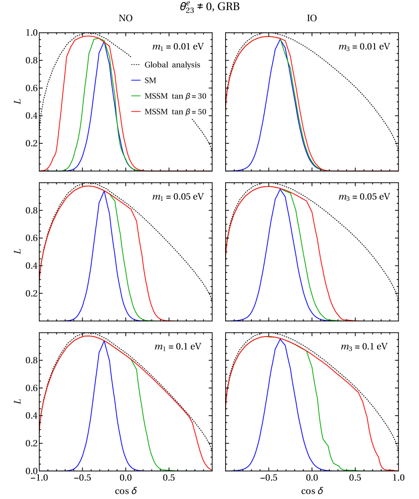
Figure 19: Likelihood function vs. $\cos\delta$ in the case of non-zero $\theta^{e}_{23}$ for the GRB symmetry form of the matrix $\tilde{U}_{\nu}$ in all the setups considered. The dotted line stands for likelihood extracted from the global analysis in [7]. The blue line is for the SM running. Finally, the green and red lines are for the running within MSSM with $\tan\beta=30$ and $\tan\beta=50$, respectively.

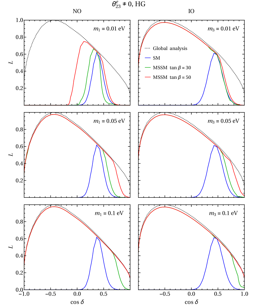
Figure 20: Likelihood function vs. $\cos\delta$ in the case of non-zero $\theta^{e}_{23}$ for the HG symmetry form of the matrix $\tilde{U}_{\nu}$ in all the setups considered. The dotted line stands for likelihood extracted from the global analysis in [7]. The blue line is for the SM running. Finally, the green and red lines are for the running within MSSM with $\tan\beta=30$ and $\tan\beta=50$, respectively.

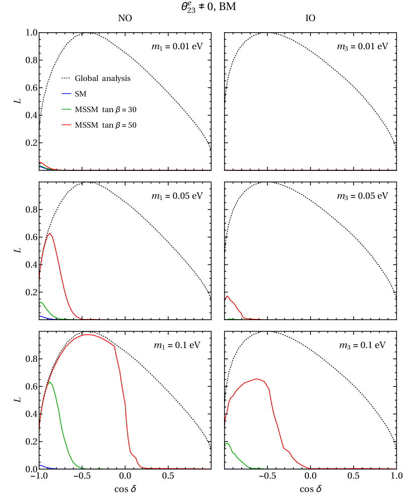
Figure 21: Likelihood function vs. $\cos\delta$ in the case of non-zero $\theta^{e}_{23}$ for the BM symmetry form of the matrix $\tilde{U}_{\nu}$ in all the setups considered. The dotted line stands for likelihood extracted from the global analysis in [7]. The blue line is for the SM running. Finally, the green and red lines are for the running within MSSM with $\tan\beta=30$ and $\tan\beta=50$, respectively.

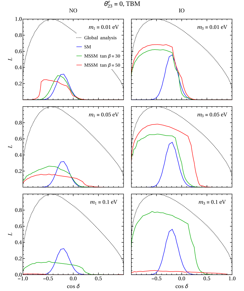
Figure 22: Likelihood function vs. $\cos\delta$ in the case of zero $\theta^{e}_{23}$ for the TBM symmetry form of the matrix $\tilde{U}_{\nu}$ in all the setups considered. The dotted line stands for likelihood extracted from the global analysis in [7]. The blue line is for the SM running. Finally, the green and red lines are for the running within MSSM with $\tan\beta=30$ and $\tan\beta=50$, respectively.

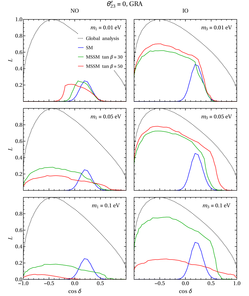
Figure 23: Likelihood function vs. $\cos\delta$ in the case of zero $\theta^{e}_{23}$ for the GRA symmetry form of the matrix $\tilde{U}_{\nu}$ in all the setups considered. The dotted line stands for likelihood extracted from the global analysis in [7]. The blue line is for the SM running. Finally, the green and red lines are for the running within MSSM with $\tan\beta=30$ and $\tan\beta=50$, respectively.

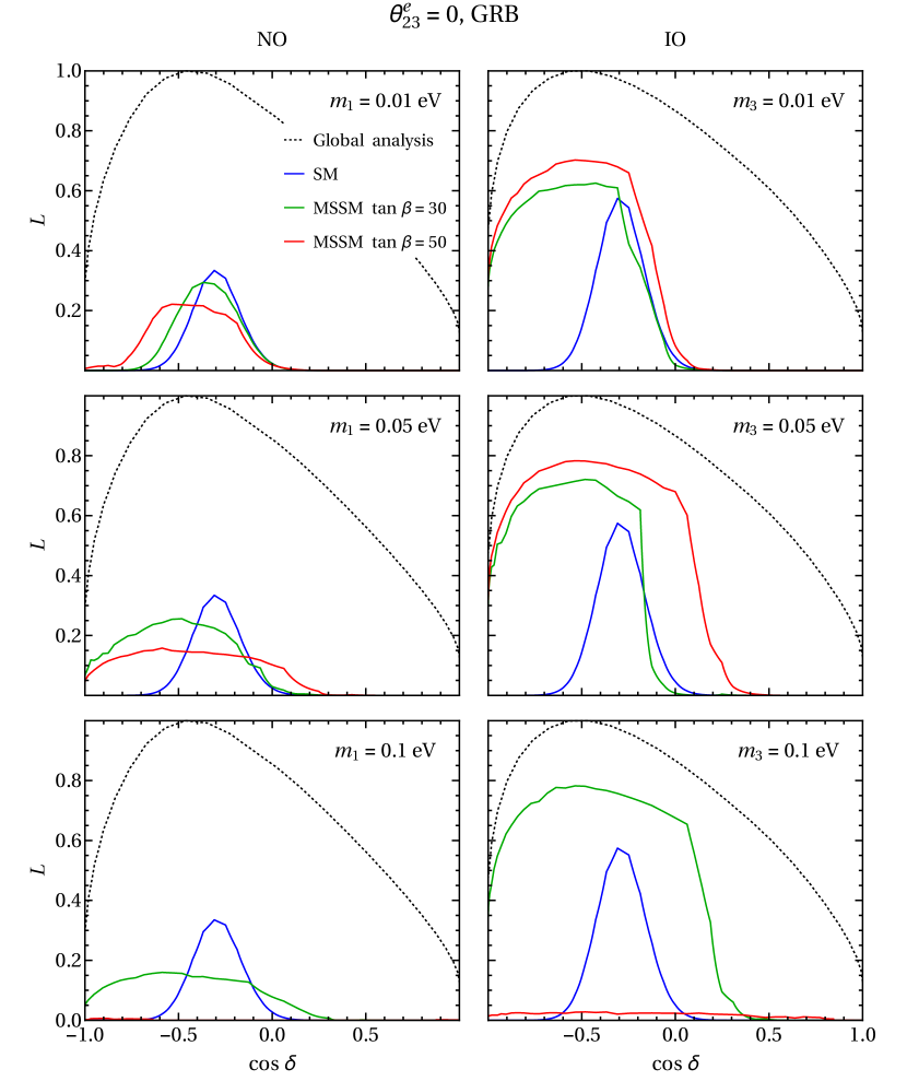
Figure 24: Likelihood function vs. $\cos\delta$ in the case of zero $\theta^{e}_{23}$ for the GRB symmetry form of the matrix $\tilde{U}_{\nu}$ in all the setups considered. The dotted line stands for likelihood extracted from the global analysis in [7]. The blue line is for the SM running. Finally, the green and red lines are for the running within MSSM with $\tan\beta=30$ and $\tan\beta=50$, respectively.

Figure 25: Likelihood function vs. $\cos\delta$ in the case of zero $\theta^{e}_{23}$ for the HG symmetry form of the matrix $\tilde{U}_{\nu}$ in all the setups considered. The dotted line stands for likelihood extracted from the global analysis in [7]. The blue line is for the SM running. Finally, the green and red lines are for the running within MSSM with $\tan\beta=30$ and $\tan\beta=50$, respectively.

References

- [1] H. Ishimori et al., Prog. Theor. Phys. Suppl. 183 (2010) 1 [arXiv:1003.3552 [hep-th]].
- [2] G. Altarelli and F. Feruglio, Rev. Mod. Phys. 82 (2010) 2701 [arXiv:1002.0211 [hep-ph]].
- [3] S. F. King and C. Luhn, Rept. Prog. Phys. 76 (2013) 056201 [arXiv:1301.1340 [hep-ph]].
- [4] S. F. King et al., New J. Phys. 16 (2014) 045018 [arXiv:1402.4271 [hep-ph]].
- [5] K. Nakamura and S. T. Petcov, in C. Patrignani et al. (Particle Data Group), Chin. Phys. C 40 (2016) 100001.
- [6] S. M. Bilenky, J. Hosek and S. T. Petcov, Phys. Lett. B 94 (1980) 495.
- [7] F. Capozzi et al., Nucl. Phys. B 908 (2016) 218 [arXiv:1601.07777 [hep-ph]].
- [8] F. Capozzi et al., Phys. Rev. D 89 (2014) 093018 [arXiv:1312.2878 [hep-ph]].
- [9] M. C. Gonzalez-Garcia, M. Maltoni and T. Schwetz, JHEP 1411 (2014) 052 [arXiv:1409.5439 [hep-ph]].
- [10] A. D. Hanlon, S. F. Ge and W. W. Repko, Phys. Lett. B 729 (2014) 185 [arXiv:1308.6522 [hep-ph]]; S. F. Ge, D. A. Dicus and W. W. Repko, Phys. Rev. Lett. 108 (2012) 041801 [arXiv:1108.0964 [hep-ph]]; S. F. Ge, D. A. Dicus and W. W. Repko, Phys. Lett. B 702 (2011) 220 [arXiv:1104.0602 [hep-ph]].
- [11] D. Marzocca, S. T. Petcov, A. Romanino and M. C. Sevilla, JHEP 1305 (2013) 073 [arXiv:1302.0423 [hep-ph]].
- [12] S. T. Petcov, Nucl. Phys. B 892 (2015) 400 [arXiv:1405.6006 [hep-ph]].
- [13] I. Girardi, S. T. Petcov and A. V. Titov, Nucl. Phys. B 894 (2015) 733 [arXiv:1410.8056 [hep-ph]].
- [14] I. Girardi, S. T. Petcov and A. V. Titov, Int. J. Mod. Phys. A 30 (2015) 1530035 [arXiv:1504.02402 [hep-ph]].
- [15] I. Girardi, S. T. Petcov and A. V. Titov, Eur. Phys. J. C 75 (2015) 345 [arXiv:1504.00658 [hep-ph]].
- [16] I. Girardi, S. T. Petcov, A. J. Stuart and A. V. Titov, Nucl. Phys. B 902 (2016) 1 [arXiv:1509.02502 [hep-ph]].
- [17] I. Girardi, S. T. Petcov and A. V. Titov, Nucl. Phys. B 911 (2016) 754 [arXiv:1605.04172 [hep-ph]].
- [18] S. F. King, A. Merle and A. J. Stuart, JHEP 1312 (2013) 005 [arXiv:1307.2901 [hep-ph]]; M. Agostini, A. Merle and K. Zuber, Eur. Phys. J. C 76 (2016) no.4, 176 [arXiv:1506.06133 [hep-ex]]; J. Gehrlein, A. Merle and M. Spinrath, Phys. Rev. D 94 (2016) 093003 [arXiv:1606.04965 [hep-ph]].
- [19] J. Gehrlein, A. Merle and M. Spinrath, JHEP 1509 (2015) 066 [arXiv:1506.06139 [hep-ph]].
- [20] S. Antusch, J. Kersten, M. Lindner and M. Ratz, Nucl. Phys. B 674 (2003) 401 [hep-ph/0305273].
- [21] M. A. Schmidt and A. Y. Smirnov, Phys. Rev. D 74 (2006) 113003 [hep-ph/0607232].
- [22] S. Boudjemaa and S. F. King, Phys. Rev. D 79 (2009) 033001 [arXiv:0808.2782 [hep-ph]].
- [23] S. T. Petcov, Phys. Lett. B 110 (1982) 245; F. Vissani, hep-ph/9708483; V. D. Barger, S. Pakvasa, T. J. Weiler and K. Whisnant, Phys. Lett. B 437 (1998) 107 [hep-ph/9806387]; A. J. Baltz, A. S. Goldhaber and M. Goldhaber, Phys. Rev. Lett. 81 (1998) 5730 [hep-ph/9806540].
- [24] Z. z. Xing, Phys. Lett. B 533 (2002) 85 [hep-ph/0204049]; P. F. Harrison, D. H. Perkins and W. G. Scott, Phys. Lett. B 530 (2002) 167 [hep-ph/0202074]; P. F. Harrison and W. G. Scott, Phys. Lett. B 535 (2002) 163 [hep-ph/0203209]; X. G. He and A. Zee, Phys. Lett. B 560 (2003) 87 [hep-ph/0301092].
- [25] L. Wolfenstein, Phys. Rev. D 18 (1978) 958.
- [26] S. Antusch, S. F. King and M. Malinsky, Nucl. Phys. B 820 (2009) 32 [arXiv:0810.3863 [hep-ph]].
- [27] P. Ballett et al., JHEP 1412 (2014) 122 [arXiv:1410.7573 [hep-ph]].
- [28] Y. Kajiyama, M. Raidal and A. Strumia, Phys. Rev. D 76 (2007) 117301 [arXiv:0705.4559 [hep-ph]]; L. L. Everett and A. J. Stuart, Phys. Rev. D 79 (2009) 085005 [arXiv:0812.1057 [hep-ph]].
- [29] W. Rodejohann, Phys. Lett. B 671 (2009) 267 [arXiv:0810.5239 [hep-ph]]; A. Adulpravitchai, A. Blum and W. Rodejohann, New J. Phys. 11 (2009) 063026 [arXiv:0903.0531 [hep-ph]].
- [30] C. H. Albright, A. Dueck and W. Rodejohann, Eur. Phys. J. C 70 (2010) 1099 [arXiv:1004.2798 [hep-ph]]; J. E. Kim and M. S. Seo, JHEP 1102 (2011) 097 [arXiv:1005.4684 [hep-ph]].
- [31] J. Zhang and S. Zhou, JHEP 1608 (2016) 024 [arXiv:1604.03039 [hep-ph]].
- [32] P. H. Frampton, S. T. Petcov and W. Rodejohann, Nucl. Phys. B 687 (2004) 31 [hep-ph/0401206].
- [33] J. Gehrlein, J. P. Oppermann, D. Schäfer and M. Spinrath, Nucl. Phys. B 890 (2014) 539 [arXiv:1410.2057 [hep-ph]]; J. Gehrlein, S. T. Petcov, M. Spinrath and X. Zhang, Nucl. Phys. B 896 (2015) 311 [arXiv:1502.00110 [hep-ph]]; J. Gehrlein, S. T. Petcov, M. Spinrath and X. Zhang, Nucl. Phys. B 899 (2015) 617 [arXiv:1508.07930 [hep-ph]].
- [34] A. Meroni, S. T. Petcov and M. Spinrath, Phys. Rev. D 86 (2012) 113003 [arXiv:1205.5241 [hep-ph]].
- [35] D. Marzocca, S. T. Petcov, A. Romanino and M. Spinrath, JHEP 1111 (2011) 009 [arXiv:1108.0614 [hep-ph]].
- [36] S. Antusch, C. Gross, V. Maurer and C. Sluka, Nucl. Phys. B 866 (2013) 255 [arXiv:1205.1051 [hep-ph]].
- [37] S. Antusch, S. F. King and M. Spinrath, Phys. Rev. D 87 (2013) 096018 [arXiv:1301.6764 [hep-ph]].
- [38] S. Antusch, S. F. King and M. Spinrath, Phys. Rev. D 83 (2011) 013005 [arXiv:1005.0708 [hep-ph]].
- [39] I. Girardi, A. Meroni, S. T. Petcov and M. Spinrath, JHEP 1402 (2014) 050 [arXiv:1312.1966 [hep-ph]].
- [40] S. Antusch et al., JHEP 0503 (2005) 024 [hep-ph/0501272].
- [41] S. Antusch, S. F. King, C. Luhn and M. Spinrath, Nucl. Phys. B 850 (2011) 477 [arXiv:1103.5930 [hep-ph]].
- [42] S. M. Bilenky, S. Pascoli and S. T. Petcov, Phys. Rev. D 64 (2001) 053010 [hep-ph/0102265]; S. T. Petcov, Adv. High Energy Phys. 2013 (2013) 852987 [arXiv:1303.5819 [hep-ph]].
- [43] L. J. Hall, R. Rattazzi and U. Sarid, Phys. Rev. D 50 (1994) 7048 [arXiv:hep-ph/9306309]; M. S. Carena, M. Olechowski, S. Pokorski and C. E. M. Wagner, Nucl. Phys. B 426 (1994) 269 [arXiv:hep-ph/9402253]; R. Hempfling, Phys. Rev. D 49 (1994) 6168; T. Blazek, S. Raby and S. Pokorski, Phys. Rev. D 52 (1995) 4151 [arXiv:hep-ph/9504364].
- [44] P. A. R. Ade et al. [Planck Collaboration], Astron. Astrophys. 594 (2016) A13 [arXiv:1502.01589 [astro-ph.CO]].