Quantum-statistical approach to electromagnetic wave propagation and dissipation inside dielectric media and nanophotonic and plasmonic waveguides

Abstract

Quantum-statistical effects occur during the propagation of electromagnetic (EM) waves inside the dielectric media or metamaterials, which include a large class of nanophotonic and plasmonic waveguides with dissipation and noise. Exploiting the formal analogy between the Schrödinger equation and the Maxwell equations for dielectric linear media, we rigorously derive the effective Hamiltonian operator which describes such propagation. This operator turns out to be essentially non-Hermitian in general, and pseudo-Hermitian in some special cases. Using the density operator approach for general non-Hermitian Hamiltonians, we derive a master equation that describes the statistical ensembles of EM wave modes. The method also describes the quantum dissipative and decoherence processes which happen during the wave’s propagation, and, among other things, it reveals the conditions that are necessary to control the energy and information loss inside the above-mentioned materials.

I Introduction

Notwithstanding the long history of studies, the propagation of electromagnetic (EM) wave inside dielectric media remains an important and rapidly developing topic. Apart from an obvious theoretical value, it finds numerous applications in the designs of the nanoscale photonic and plasmonic devices, structures and metamaterials, such as lasers, spasers, modulators, waveguides, optical switches, laser-absorbers, coupled resonators and quantum wells.

During the past decade there has been growing interest in studying those systems by means of the formal analogy between Maxwell equations in dielectric media and Schrödinger-type equations, dubbed here as the Maxwell-Schrödinger (MS) map jbook65 ; kbbook72 ; wbook91 . In this analogy, Maxwell equations are rewritten in the form of the matrix Schrödinger equation, except that the role of time is played by the coordinate along the direction of wave propagation (usually, $z$-coordinate), the Hamiltonian operator is non-Hermitian (NH), and the Planck constant is replaced by an effective one sybook09 . Therefore, a class of the physical systems that allow such mapping is broadly referred as non-Hermitian materials and waveguides. Moreover, inside this class one can select the subclass of physical systems and phenomena for which the above-mentioned Hamiltonian operator has real spectrum, in which case it is called pseudo-Hermitian ml08 ; zhu11 . This pseudo-Hermiticity manifests itself in various phenomena, such as non-reciprocal light propagation and Bloch oscillations yz13 ; fah11 ; lo09 , invisibility and loss-induced transparency lo11 ; lre11 ; fxf13 ; kcl14 ; gsd09 , power oscillations mec08 ; rme10 ; rbm12 , optical switching csp92 ; sxk10 ; lbd13 , coherent perfect absorptions cgc10 ; fh12 ; stl14 , laser-absorbers lo10 ; cgs11 , plasmonic waveguides ad14 , unidirectional tunneling scg14 , loss-free negative refraction fsa14 , and so on. These processes can be studied using a general theory of pseudo-Hermitian (often referred also as ${\cal PT}$-symmetric) Hamiltonians, which has originated from works jd61 ; sgh92 ; ben98 , one could mention also the classical results by Dyson fd56 ; jof71 .

However, the class of non-Hermitian materials and waveguides is obviously much larger than its pseudo-Hermitian subclass. Indeed, as a result of the interaction of EM waves with their environment (which can be very diverse and uncontrollable), the description of their propagation requires the usage of the NH Hamiltonians of different kinds, not necessarily possessing real eigenvalues. In other words, this propagation must be described within the framework of a general theory of open quantum systems bpbook . According to that theory, for such situations one needs to engage the full description of the (quantum) statistical ensemble of EM wave modes. In turn, it requires the usage of the density matrix, instead of a state vector, as a main object of theory. Therefore, MS map must be used to develop the corresponding generalization, which is going to be the main goal of this paper . Although the density-operator approach for quantum systems driven by NH Hamiltonians has been long since known (see, for instance, the monograph fbook ), it has been further developed in the works sz13 ; sz14 ; sz14cor ; ser15 ; sz15 ; zlo15 . In the current paper we adapt this formalism for the purposes of describing the EM wave propagation inside dielectric materials and waveguides in presence of dissipative effects induced by environment, as well as for extracting physical information and predicting new phenomena.

The contents of this paper are as follows. In section II, we provide essential information about the Maxwell-Schrödinger map for EM wave propagation inside dielectric linear media of a general type. We define the appropriate Hilbert space, as well as we introduce notions and representations, which will be necessary for what follows. In section III, we formulate the density matrix approach for NH dynamics adapted for the MS-mapped models and NH waveguides with dissipation of general type. We derive a master equation, which governs the statistical behavior of EM wave modes inside the medium, and describe its properties. In section IV, we use the properties of the Hilbert space in our case in order to introduce the two-level approach to deriving quantum-statistical observables for any given medium. This approach reveals more details about physical features of the systems which are being studied, as well as it explicitly illustrates some statistical effects that occur. Discussions and conclusions are given in section V.

II Maxwell-Schrödinger analogy in dielectric media

In this section, we formulate the formal mapping between certain classes of Maxwell and Schrödinger equations. We rigorously derive the effective Hamiltonian operator, which describes the propagation of EM waves in dielectric isotropic media along a certain direction. Due to its generality, the approach is applicable for studying EM wave propagation inside a very large class of materials where at least one preferred direction of propagation can be established.

II.1 Effective Hamiltonian

Let us consider EM wave propagating inside a dielectric isotropic linear medium. For this situation, there are no free charges and currents, therefore, Maxwell equations acquire a simple form:

$$\boldsymbol{\nabla}\times\mathbf{E}+\frac{1}{c}\frac{\partial}{\partial t}(\mu\mathbf{H})=0,$$ (1a)

$$\boldsymbol{\nabla}\times\mathbf{H}-\frac{1}{c}\frac{\partial}{\partial t}(\varepsilon\mathbf{E})=0,$$ (1b)

$$\boldsymbol{\nabla}\cdot(\varepsilon\mathbf{E})=\boldsymbol{\nabla}\cdot(\mu\mathbf{H})=0,$$ (1c)

where $\mathbf{E}=\mathbf{E}(\mathbf{r},t)$ and $\mathbf{H}=\mathbf{H}(\mathbf{r},t)$ are electric and magnetic fields, respectively, while the cross and dot denote the vector and scalar products, respectively. Here $c=1/\sqrt{\varepsilon_{0}\mu_{0}}$, $\varepsilon_{0}$ and $\mu_{0}$ being, respectively, the vacuum permittivity and permeability, whereas $\varepsilon$ and $\mu$ are the relative permittivity and permeability (complex-valued functions of coordinates, in general); as per usual, one can also express them via the medium’s electric and magnetic susceptibilities: $\varepsilon=1+\chi_{e}$ and $\mu=1+\chi_{m}$. The electromagnetic Gaussian unit system’s conventions can be used here, as long as the physical vacuum is assumed to be fixed in its current state characterized by the adopted SI values of $\varepsilon_{0}$ and $\mu_{0}$.

Further, if we align $z$-axis with the direction of wave’s propagation then, assuming the harmonic time dependence of the electric and magnetic fields,

$$\mathbf{E}(\mathbf{r},t)=\mathbf{E}(x,y,z)\exp{(-i\omega t)},$$ (2a)

$$\mathbf{H}(\mathbf{r},t)=\mathbf{H}(x,y,z)\exp{(-i\omega t)},$$ (2b)

one can decompose them into the transverse and longitudinal (along $z$-axis) components: $\mathbf{E}=\mathbf{E}_{\bot}+\mathbf{e}_{z}E_{z}$, $\mathbf{H}=\mathbf{H}_{\bot}+\mathbf{e}_{z}H_{z}$, $\boldsymbol{\nabla}=\boldsymbol{\nabla}_{\bot}+\mathbf{e}_{z}\frac{\partial}{\partial z}$, where $\mathbf{e}_{n}$ is the basis vector along the $n$th axis. One can show that the vectors $\mathbf{E}_{\bot}$ and $\mathbf{H}_{\bot}$ are essentially two-dimensional: $\mathbf{E}_{\bot}\cdot\mathbf{e}_{z}=\mathbf{H}_{\bot}\cdot\mathbf{e}_{z}=0$. Correspondingly, Maxwell equations take the form (from now on we adopt the units where $c=1$)

$$\frac{\partial}{\partial z}\mathbf{E}_{\bot}-\boldsymbol{\nabla}_{\bot}E_{z}+i\mu\omega(\mathbf{e}_{z}\times\mathbf{H}_{\bot})=0,$$ (3a)

$$\frac{\partial}{\partial z}\mathbf{H}_{\bot}-\boldsymbol{\nabla}_{\bot}H_{z}-i\varepsilon\omega(\mathbf{e}_{z}\times\mathbf{E}_{\bot})=0,$$ (3b)

$$\mathbf{e}_{z}\cdot\left(\boldsymbol{\nabla}_{\bot}\times\mathbf{H}_{\bot}\right)+i\varepsilon\omega E_{z}=0,$$ (3c)

$$\mathbf{e}_{z}\cdot\left(\boldsymbol{\nabla}_{\bot}\times\mathbf{E}_{\bot}\right)-i\mu\omega H_{z}=0,$$ (3d)

$$\frac{\partial}{\partial z}\left(\varepsilon E_{z}\right)+\boldsymbol{\nabla}_{\bot}\cdot\left(\varepsilon\mathbf{E}_{\bot}\right)=0,$$ (3e)

$$\frac{\partial}{\partial z}\left(\mu H_{z}\right)+\boldsymbol{\nabla}_{\bot}\cdot\left(\mu\mathbf{H}_{\bot}\right)=0,$$ (3f)

and also for definiteness we assume throughout the paper that the medium is located at $z\geqslant 0$.

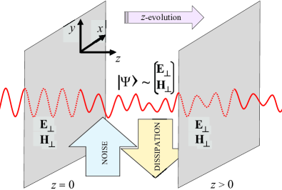
Figure 1: Propagation of EM wave through a dielectric medium located at $z\geqslant 0$.

The system (3) can be recast in the form, in which the equations for longitudinal and transverse vectors are explicitly separated:

$$i\mathbf{e}_{z}\times\frac{\partial}{\partial z}\mathbf{E}_{\bot}=\hat{L}_{m}\mathbf{H}_{\bot},$$ (4a)

$$i\mathbf{e}_{z}\times\frac{\partial}{\partial z}\mathbf{H}_{\bot}=-\hat{L}_{e}\mathbf{E}_{\bot},$$ (4b)

$$E_{z}=(i\varepsilon\omega)^{-1}\mathbf{e}_{z}\cdot\left(\boldsymbol{\nabla}_{\bot}\times\mathbf{H}_{\bot}\right),$$ (4c)

$$H_{z}=-(i\mu\omega)^{-1}\mathbf{e}_{z}\cdot\left(\boldsymbol{\nabla}_{\bot}\times\mathbf{E}_{\bot}\right),$$ (4d)

where we denote the following differential operators:

$$\hat{L}_{e}=\varepsilon\omega-\omega^{-1}\boldsymbol{\nabla}_{\bot}\times\mu^{-1}\boldsymbol{\nabla}_{\bot}\times,$$ (5a)

$$\hat{L}_{m}=\mu\omega-\omega^{-1}\boldsymbol{\nabla}_{\bot}\times\varepsilon^{-1}\boldsymbol{\nabla}_{\bot}\times.$$ (5b)

Using the 2D property $\mathbf{e}_{z}\times\mathbf{e}_{z}\times=-1$, the equations (4a) and (4b) can be written in the matrix form

$$i\frac{\partial}{\partial z}{\mathbf{E}_{\bot}\choose{\mathbf{H}_{\bot}}}=\hat{h}{\mathbf{E}_{\bot}\choose{\mathbf{H}_{\bot}}},$$ (6)

where we denote the operator

$$\hat{h}=\hat{\sigma}_{2}\hat{\cal D}=\begin{pmatrix}0&-\mathbf{e}_{z}\times\hat{L}_{m}\\ \mathbf{e}_{z}\times\hat{L}_{e}&0\end{pmatrix},$$ (7)

where $\hat{\sigma}_{2}$ is defined in Appendix A, and

$$\hat{\cal D}\equiv\hat{\sigma}_{2}\hat{h}=\begin{pmatrix}\hat{L}_{e}&0\\ 0&\hat{L}_{m}\end{pmatrix}$$ (8)

is the auxiliary operator. A schematic drawing of the EM wave propagation as the wave function’s evolution along $z$-direction is shown in Fig. 1.

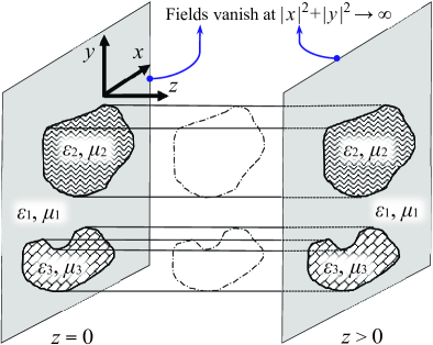
(a) Uniform waveguide

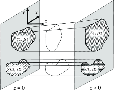
(b) General waveguide

Figure 2: EM wave propagation along $z$-direction for different kinds of media. Vertical planes represent the generalized waveguide’s effective cross-section, at different values of $z$. For a general medium, deviations from uniformity arise due to varying cross-section (wave-shaded areas on the lower panel) or varying permittivity and/or permeability (brick-shaded areas on the lower panel).

Furthermore, using the formulas from Appendix A, one can check that the operator (7) is non-Hermitian, even when both $\varepsilon$ and $\mu$ are real-valued. This holds for either a uniform waveguide type geometry [Fig. 2a] or for a more general non uniform geometry [Fig. 2b], as long as the issue of transverse fields vanishing at spatial infinity is properly satisfied, as we will discuss later. The degree of non-Hermiticity of the theory’s Hamiltonian becomes even larger if we write (6) in the form that is fully analogous to the Schrödinger equation, for we must rewrite it in terms of normalized values. Defining an inner product as the integral over what we can call the generalized waveguide’s effective cross-section (i.e., the region outside of which the EM wave’s fields vanish, cf. Fig. 2), one can introduce the normalization factor

$${\cal N}^{2}\equiv\int d\textbf{x}_{\bot}\left(\left|\mathbf{E}_{\bot}\right|^{2}+\left|\mathbf{H}_{\bot}\right|^{2}\right),$$ (9)

where $d\textbf{x}_{\bot}$ would be $dxdy$ in Cartesian coordinates. Function ${\cal N}$ does not depend on the transverse coordinates but in general it can depend on $z$. With these definitions in hand, we can define the following wavefunction (using the Dirac’s bra-ket notations):

$$\Psi\equiv\left\langle\textbf{x}_{\bot}|\Psi\right\rangle=\frac{1}{{\cal N}}{\mathbf{E}_{\bot}\choose{\mathbf{H}_{\bot}}},$$ (10)

which is automatically normalized to one

$$\left\langle\Psi|\Psi\right\rangle=1,$$ (11)

and thus the corresponding state vector $|\Psi\rangle$ can be regarded as a ray in some appropriate Hilbert space (defined in Sec. II.3 below). In terms of this state vector, Eq. (6) acquires the Schrödinger equation’s form

$$i\hbar_{\text{w}}\frac{\partial}{\partial z}\Psi=\hat{\cal H}\Psi,$$ (12)

where we denote the operator

$$\hat{\cal H} \equiv \hbar_{\text{w}}\left(\hat{h}+\hat{\cal H}_{\cal N}\right)=\hbar_{\text{w}}\left(\hat{\sigma}_{2}\hat{\cal D}-i\Gamma_{\cal N}\hat{\cal{I}}\right)$$ (13)

$$= \hbar_{\text{w}}\begin{pmatrix}0&-\mathbf{e}_{z}\times\hat{L}_{m}\\ \mathbf{e}_{z}\times\hat{L}_{e}&0\end{pmatrix}-i\hbar_{\text{w}}\Gamma_{\cal N}\begin{pmatrix}\hat{I}&~{}0\\ 0&~{}\hat{I}\end{pmatrix}\!,~{}~{}~{}$$

where $\hat{\cal{I}}$ and $\hat{I}$ are, respectively, the identity operator and the $2\times 2$ identity matrix, and the coefficient

$$\Gamma_{\cal N}=\frac{\partial}{\partial z}\ln{|{\cal N}|}$$ (14)

is in general a real-valued function of $z$ (as well as a functional of the fields); if ${\cal N}$ do vary with $z$ then Eq. (12) is not merely a rescaled version of Eq. (6) but involves a corrective term, in general. Here by $z$ we assume the value $z/c$, and the “Planck” constant $\hbar_{\text{w}}$ is an effective scale constant of the dimensionality energy$\times$time, which is introduced for a purpose of preserving the correct dimensionality of the relevant terms in the emergent Schrödinger equation (the ambiguity of $\hbar_{\text{w}}$ is yet another manifestation of the absence of the fundamental length scale in Maxwell equations sybook09 ). Following traditions, we will refer to the operator (13) as the Hamiltonian operator of the system, although, strictly speaking, a non-Hermitian operator cannot be fully regarded as Hamiltonian: the anti-Hermitian part of such an operator does not correspond to any symplectic structure but rather plays a special role which will be discussed in Sec. III.1 below. It should be also noted that in a case when free charges or currents exist in the medium, the original Maxwell equations of Sec. II.1 must be modified, which can result either in a different expression for our analogous Hamiltonian or in a breakdown of the Maxwell-Schrödinger analogy as such. In this paper, we assume such charges and currents to be sufficiently small and consider a leading-order approximation.

Furthermore, it should be noticed the appearance of the additional term in the Hamiltonian (13), $\hat{\cal H}_{\cal N}\equiv-i\Gamma_{\cal N}\hat{\cal{I}}=-i\Gamma_{\cal N}\left(\begin{smallmatrix}\hat{I}&~{}0\\ 0&~{}\hat{I}\end{smallmatrix}\right),$ which is essentially anti-Hermitian and proportional to the identity operator. Due to the latter feature, it belongs to the class of the Hamiltonian “gauge” terms, which role’s discussion will be postponed until Sec. III.6.

Thus, equations (10)-(13) represent the formal map between Maxwell equations for dielectric linear media and the differential equation of the Schrödinger type, which opens up the possibility of using quantum mechanical notions (with certain provisions of course) for the purposes of a theory of EM wave propagation inside different dielectric materials, including waveguides.

II.2 Basic features of Hamiltonian

Let us consider now the operator (7). Its Hermitian conjugate is given by

$$\hat{h}^{\dagger}=\hat{\cal D}^{\dagger}\hat{\sigma}_{2}=\begin{pmatrix}0&-\hat{L}_{e}^{\dagger}\mathbf{e}_{z}\times\\ \hat{L}_{m}^{\dagger}\mathbf{e}_{z}\times&0\end{pmatrix},$$ (15)

where

$$\hat{L}_{e}^{\dagger}=\varepsilon^{*}\omega-\omega^{-1}\boldsymbol{\nabla}_{\bot}\times\frac{1}{\mu^{*}}\boldsymbol{\nabla}_{\bot}\times,$$ (16a)

$$\hat{L}_{m}^{\dagger}=\mu^{*}\omega-\omega^{-1}\boldsymbol{\nabla}_{\bot}\times\frac{1}{\varepsilon^{*}}\boldsymbol{\nabla}_{\bot}\times,$$ (16b)

hence, it is clear that $\hat{h}\not=\hat{h}^{\dagger}$ even if the $L$-operators are both self-adjoint (which happens in the case $\mu=\mu^{*}$ and $\varepsilon=\varepsilon^{*}$, which will be discussed in what follows), as $\hat{L}^{\dagger}$ now appears on the right side of the curl. The only difference between the case of real-valued $\varepsilon$ and $\mu$ and the general one (when either or both $\varepsilon$ and $\mu$ are complex) is that the operator $\hat{h}$ is pseudo-Hermitian in the former case and strongly non-Hermitian in the latter. The eigenvalues of a pseudo-Hermitian operator are real-valued, whereas the ones of a general non-Hermitian operator are complex. Indeed, the case of real $\varepsilon$ and $\mu$ is a special one because then

$$\hat{h}^{\dagger}=\begin{pmatrix}0&-\hat{L}_{e}\mathbf{e}_{z}\times\\ \hat{L}_{m}\mathbf{e}_{z}\times&0\end{pmatrix},\ \ \forall\ \varepsilon,\mu\in\Re,$$ (17)

such that the following identity takes place

$$\hat{h}^{\dagger}\hat{\sigma}_{2}-\hat{\sigma}_{2}\hat{h}=\hat{\cal D}^{\dagger}-\hat{\cal D}=0,\ \ \forall\ \varepsilon,\mu\in\Re,$$ (18)

which confirms that the operator $\hat{h}$ is pseudo-Hermitian with $\hat{\sigma}_{2}$ playing a role of the intertwining operator zhu11 . Alternatively, using (9) and (10), one can check that the expectation value of the operator $\hat{\sigma}_{2}\hat{h}$ is real-valued when the values $\varepsilon$ and $\mu$ are — since in that case the operator $\hat{\cal D}$ is self-adjoint, cf. Eq. (8).

Besides, we can also derive that

$$\hat{\sigma}_{1}\hat{h}=i\begin{pmatrix}\hat{L}_{e}&0\\ 0&-\hat{L}_{m}\end{pmatrix},$$ (19)

$$(\hat{\sigma}_{1}\hat{h})^{\dagger}\equiv\hat{h}^{\dagger}\hat{\sigma}_{1}=-\hat{\sigma}_{1}\hat{h},\ \ \forall\ \varepsilon,\mu\in\Re,$$ (20)

$$\hat{\sigma}_{3}\hat{h}=-\hat{h}\hat{\sigma}_{3}=-\begin{pmatrix}0&\mathbf{e}_{z}\times\hat{L}_{m}\\ \mathbf{e}_{z}\times\hat{L}_{e}&0\end{pmatrix},$$ (21)

such that

$$\left\{\hat{\sigma}_{3},\hat{h}\right\}=\left\{\hat{\sigma}_{3},\hat{\sigma}_{2}\hat{\cal D}\right\}=\hat{\sigma}_{2}\left[\hat{\cal D},\hat{\sigma}_{3}\right]=0,$$ (22)

and

$$\left[\hat{\cal D},\hat{\sigma}_{3}\right]=\left[\hat{\cal D}^{\dagger},\hat{\sigma}_{3}\right]=0,\ \ \forall\ \varepsilon,\mu\in\Re.$$ (23)

The last two equations become identities in the case of a diagonal matrix $\hat{\cal D}$.

For further developments it will be convenient to know the expectation values of the products of operators that involve $\hat{h}$, as well as their relations to the EM fields. Using the formulas above, we obtain

$$\langle\hat{h}\rangle_{\Psi} = \frac{\omega}{{\cal N}^{2}}\int dxdy\left[\varepsilon\mathbf{H}_{\bot}^{*}\cdot(\mathbf{e}_{z}\times\mathbf{E}_{\bot})-\mu\mathbf{E}_{\bot}^{*}\cdot(\mathbf{e}_{z}\times\mathbf{H}_{\bot})\right]-\frac{i}{{\cal N}^{2}}\int dxdy\left[E_{z}(\boldsymbol{\nabla}_{\bot}\cdot\mathbf{E}_{\bot}^{*})+H_{z}(\boldsymbol{\nabla}_{\bot}\cdot\mathbf{H}_{\bot}^{*})\right]$$ (24)

$$= \frac{\omega}{{\cal N}^{2}}\int dxdy\left(\varepsilon E_{[x}H_{y]}^{*}+\mu E_{[x}^{*}H_{y]}\right)-\frac{i}{{\cal N}^{2}}\int dxdy\left[E_{z}(\boldsymbol{\nabla}_{\bot}\cdot\mathbf{E}_{\bot}^{*})+H_{z}(\boldsymbol{\nabla}_{\bot}\cdot\mathbf{H}_{\bot}^{*})\right],$$

$$\langle\hat{\sigma}_{1}\hat{h}\rangle_{\Psi} = i\frac{\omega}{{\cal N}^{2}}\int dxdy\left(\varepsilon|\mathbf{E}_{\bot}|^{2}-\mu|\mathbf{H}_{\bot}|^{2}+\varepsilon^{*}|E_{z}|^{2}-\mu^{*}|H_{z}|^{2}\right),$$ (25)

$$\langle\hat{\sigma}_{2}\hat{h}\rangle_{\Psi} = \langle\hat{\cal D}\rangle_{\Psi}=\frac{\omega}{{\cal N}^{2}}\int dxdy\left(\varepsilon|\mathbf{E}_{\bot}|^{2}+\mu|\mathbf{H}_{\bot}|^{2}-\varepsilon^{*}|E_{z}|^{2}-\mu^{*}|H_{z}|^{2}\right),$$ (26)

$$\langle\hat{\sigma}_{3}\hat{h}\rangle_{\Psi} = \frac{\omega}{{\cal N}^{2}}\int dxdy\left[\varepsilon\mathbf{H}_{\bot}^{*}\cdot(\mathbf{e}_{z}\times\mathbf{E}_{\bot})+\mu\mathbf{E}_{\bot}^{*}\cdot(\mathbf{e}_{z}\times\mathbf{H}_{\bot})\right]+\frac{i}{{\cal N}^{2}}\int dxdy\left[E_{z}(\boldsymbol{\nabla}_{\bot}\cdot\mathbf{E}_{\bot}^{*})-H_{z}(\boldsymbol{\nabla}_{\bot}\cdot\mathbf{H}_{\bot}^{*})\right]$$ (27)

$$= \frac{\omega}{{\cal N}^{2}}\int dxdy\left(\varepsilon E_{[x}H_{y]}^{*}-\mu E_{[x}^{*}H_{y]}\right)+\frac{i}{{\cal N}^{2}}\int dxdy\left[E_{z}(\boldsymbol{\nabla}_{\bot}\cdot\mathbf{E}_{\bot}^{*})-H_{z}(\boldsymbol{\nabla}_{\bot}\cdot\mathbf{H}_{\bot}^{*})\right],$$

and

$$\left\langle\frac{\partial}{\partial\omega}\left(\hat{\sigma}_{2}\hat{h}\right)\right\rangle_{\Psi} = \left\langle\frac{\partial}{\partial\omega}\hat{\cal D}\right\rangle_{\Psi}=\frac{1}{{\cal N}^{2}}\int dxdy\left(\varepsilon|\mathbf{E}_{\bot}|^{2}+\mu|\mathbf{H}_{\bot}|^{2}+\varepsilon^{*}|E_{z}|^{2}+\mu^{*}|H_{z}|^{2}\right),$$ (28)

and similarly for the adjoint operator:

$$\langle\hat{h}^{\dagger}\rangle_{\Psi} = \frac{\omega}{{\cal N}^{2}}\int dxdy\left[\mu^{*}\mathbf{H}_{\bot}^{*}\cdot(\mathbf{e}_{z}\times\mathbf{E}_{\bot})-\varepsilon^{*}\mathbf{E}_{\bot}^{*}\cdot(\mathbf{e}_{z}\times\mathbf{H}_{\bot})\right]+\frac{i}{{\cal N}^{2}}\int dxdy\left[E_{z}^{*}(\boldsymbol{\nabla}_{\bot}\cdot\mathbf{E}_{\bot})+H_{z}^{*}(\boldsymbol{\nabla}_{\bot}\cdot\mathbf{H}_{\bot})\right]$$ (29)

$$= \frac{\omega}{{\cal N}^{2}}\int dxdy\left(\varepsilon^{*}E^{*}_{[x}H_{y]}+\mu^{*}E_{[x}H^{*}_{y]}\right)+\frac{i}{{\cal N}^{2}}\int dxdy\left[E_{z}^{*}(\boldsymbol{\nabla}_{\bot}\cdot\mathbf{E}_{\bot})+H_{z}^{*}(\boldsymbol{\nabla}_{\bot}\cdot\mathbf{H}_{\bot})\right],$$

$$\langle\hat{\sigma}_{1}\hat{h}^{\dagger}\rangle_{\Psi} = i\frac{\omega}{{\cal N}^{2}}\int dxdy\left(\mu^{*}|\mathbf{E}_{\bot}|^{2}-\varepsilon^{*}|\mathbf{H}_{\bot}|^{2}\right)-\frac{i}{{\omega\cal N}^{2}}\int dxdy\left(\frac{1}{\varepsilon^{*}}\left|\boldsymbol{\nabla}_{\bot}\cdot\mathbf{E}_{\bot}\right|^{2}-\frac{1}{\mu^{*}}\left|\boldsymbol{\nabla}_{\bot}\cdot\mathbf{H}_{\bot}\right|^{2}\right),$$ (30)

$$\langle\hat{\sigma}_{2}\hat{h}^{\dagger}\rangle_{\Psi} = \frac{\omega}{{\cal N}^{2}}\int dxdy\left(\mu^{*}|\mathbf{E}_{\bot}|^{2}+\varepsilon^{*}|\mathbf{H}_{\bot}|^{2}\right)-\frac{1}{{\omega\cal N}^{2}}\int dxdy\left(\frac{1}{\varepsilon^{*}}\left|\boldsymbol{\nabla}_{\bot}\cdot\mathbf{E}_{\bot}\right|^{2}+\frac{1}{\mu^{*}}\left|\boldsymbol{\nabla}_{\bot}\cdot\mathbf{H}_{\bot}\right|^{2}\right),$$ (31)

$$\langle\hat{\sigma}_{3}\hat{h}^{\dagger}\rangle_{\Psi} = -\frac{\omega}{{\cal N}^{2}}\int dxdy\left[\mu^{*}\mathbf{H}_{\bot}^{*}\cdot(\mathbf{e}_{z}\times\mathbf{E}_{\bot})+\varepsilon^{*}\mathbf{E}_{\bot}^{*}\cdot(\mathbf{e}_{z}\times\mathbf{H}_{\bot})\right]-\frac{i}{{\cal N}^{2}}\int dxdy\left[E_{z}^{*}(\boldsymbol{\nabla}_{\bot}\cdot\mathbf{E}_{\bot})-H_{z}^{*}(\boldsymbol{\nabla}_{\bot}\cdot\mathbf{H}_{\bot})\right]$$ (32)

$$= \frac{\omega}{{\cal N}^{2}}\int dxdy\left(\varepsilon^{*}E^{*}_{[x}H_{y]}-\mu^{*}E_{[x}H_{y]}^{*}\right)-\frac{i}{{\cal N}^{2}}\int dxdy\left[E_{z}^{*}(\boldsymbol{\nabla}_{\bot}\cdot\mathbf{E}_{\bot})-H_{z}^{*}(\boldsymbol{\nabla}_{\bot}\cdot\mathbf{H}_{\bot})\right].$$

It is easy to see that some of these expectation values can be related to the energy density quantities of a wave mode

$$\langle\hat{\sigma}_{2}\hat{h}\rangle_{\Psi}=\langle\hat{\cal D}\rangle_{\Psi}=\frac{4\omega}{{\cal N}^{2}}\left({\cal E}_{\bot}-{\cal E}_{z}^{*}\right),$$ (33)

$$\langle{\cal L}_{+}(\hat{\sigma}_{2}\hat{h})\rangle_{\Psi}=\langle{\cal L}_{+}\hat{\cal D}\rangle_{\Psi}=\frac{8\omega}{{\cal N}^{2}}{\cal E}_{\bot},$$ (34)

$$\langle{\cal L}_{-}(\hat{\sigma}_{2}\hat{h})\rangle_{\Psi}^{*}=\langle{\cal L}_{-}\hat{\cal D}\rangle_{\Psi}^{*}=\frac{8\omega}{{\cal N}^{2}}{\cal E}_{z},$$ (35)

$$\langle{\cal L}_{+}\hat{\cal D}\rangle_{\Psi}+\langle{\cal L}_{-}\hat{\cal D}\rangle_{\Psi}^{*}=\frac{8\omega}{{\cal N}^{2}}{\cal E}_{\text{tot}},$$ (36)

where ${\cal L}_{\pm}=\omega\frac{\partial}{\partial\omega}\pm 1$ is a differential operator with respect to the frequency parameter, and

$${\cal E}_{z}=\frac{1}{4}\int dxdy\left(\varepsilon|E_{z}|^{2}+\mu|H_{z}|^{2}\right),$$ (37a)

$${\cal E}_{\bot}=\frac{1}{4}\int dxdy\left(\varepsilon|\mathbf{E}_{\bot}|^{2}+\mu|\mathbf{H}_{\bot}|^{2}\right),$$ (37b)

are, respectively, the longitudinal and transverse EM wave energy densities, such that

$${\cal E}_{\text{tot}}={\cal E}_{\bot}+{\cal E}_{z}$$ (38)

is the total energy density of a mode described by the state vector (10). Finally, one can add to this list the transmitted power ${\cal P}_{z}$ from Eq. (154b).

II.3 Hilbert space and $L$-diagonal representation

Let us consider the following auxiliary eigenvalue problem:

$$\hat{L}_{e}\mathbf{F}^{(e)}=\lambda_{e}\mathbf{F}^{(e)},$$ (39a)

$$\hat{L}_{m}\mathbf{F}^{(m)}=\lambda_{m}\mathbf{F}^{(m)},$$ (39b)

where the eigenfunctions $\mathbf{F}^{(e),(m)}$ are 2D vectors obeying the normalization condition

$$\int dxdy\left(|\mathbf{F}^{(e)}|^{2}+|\mathbf{F}^{(m)}|^{2}\right)=1,$$ (40)

as well as the boundary conditions – they must vanish either outside the medium or at the transverse spatial infinity $|x|^{2}+|y|^{2}\to+\infty$. The auxiliary eigenvalues are in general complex-valued functions of $z$ and $\omega$, $\lambda=\lambda(z,\omega)$, which also depend on the parameters inside the functions $\varepsilon(x,y,z)$ and $\mu(x,y,z)$. They can become real-valued in some cases, e.g., when the permittivity and permeability are both real-valued. In the latter case, both $L$-operators become self-adjoint, therefore, this eigenvalue problem reduces to that of the Sturm-Liouville type.

Thus, the total Hilbert space of our theory can be represented as a direct sum of the function space of the eigenvectors $\mathbf{F}^{(e),(m)}$. These spaces store, separately from each other, all electric and magnetic components of EM wave modes, which are allowed by imposed boundary conditions. Their union space thus contains the information about energy transfer between electric and magnetic components for each mode, see Appendix A for details. Below in Sec. IV.2, we will see that the auxiliary eigenvalues $\lambda_{(e),(m)}$ have distinct behaviors compared to the familiar eigenvalues of Helmholtz-type equation and their dispersion relations show the physics of waves under a different light.

Further, in this representation, the operators (7) and (8) take the form

$$\hat{\cal D} = \begin{pmatrix}\lambda_{e}\hat{I}&0\\ 0&\lambda_{m}\hat{I}\end{pmatrix}=\lambda_{-}\hat{\sigma}_{3}+\lambda_{+}\hat{\cal I},$$ (41)

$$\hat{h} = \hat{\sigma}_{2}\hat{\cal D}=i\lambda_{-}\hat{\sigma}_{1}+\lambda_{+}\hat{\sigma}_{2},$$ (42)

where

$$\lambda_{\pm}=\tfrac{1}{2}(\lambda_{e}\pm\lambda_{m}),$$ (43)

therefore, the total Hamiltonian (13) becomes

$$\hat{\cal H} = \hbar_{\text{w}}\hat{\sigma}_{2}\begin{pmatrix}\lambda_{e}\hat{I}&0\\ 0&\lambda_{m}\hat{I}\end{pmatrix}-i\hbar_{\text{w}}\Gamma_{\cal N}\begin{pmatrix}\hat{I}&~{}0\\ 0&~{}\hat{I}\end{pmatrix}$$ (44)

$$= \hbar_{\text{w}}\left(i\lambda_{-}\hat{\sigma}_{1}+\lambda_{+}\hat{\sigma}_{2}-i\Gamma_{\cal N}\hat{\cal{I}}\right)$$

$$= i\hbar_{\text{w}}\left(\lambda_{e}\hat{\sigma}_{-}-\lambda_{m}\hat{\sigma}_{+}-\Gamma_{\cal N}\hat{\cal{I}}\right),$$

where $\hat{\sigma}_{\pm}=\tfrac{1}{2}(\hat{\sigma}_{1}\pm i\hat{\sigma}_{2})$. Thus, in this representation the Hamiltonian becomes a 4$\times$4 matrix consisting of 2$\times$2 blocks.

III Statistical mechanics of wave modes

What we have done in the previous section is merely a way of rewriting Maxwell equations for waves in dielectric media in the Schrödinger form (12). In this section we will proceed with an important generalization: we go beyond those equations and adapt the quantum-type density matrix approach fbook ; sz13 ; sz14 ; sz14cor ; ser15 ; sz15 ; zlo15 for describing the propagation of EM waves inside dielectric media. This will allow us to describe not only separate wave modes (“pure states”, in quantum-mechanical terminology) or their superpositions (“entangled pure states”) but also their statistical ensembles (“mixed states”). The latter are crucial for introducing the dissipative effects since the purity of the states is not necessarily preserved in presence of dissipative environments zur96 ; zlo15 . More details will be given in Sec. III.1 below, here we only note that one should not confuse our approach with the Loudon microscopical QED-type quantization of light in presence of matter lobook ; jil93 , nor our approach is directly related to the Nyquist-Callen(-Rytov) approach to thermal fluctuational electrodynamics ryt58 . The quantum-type statistics of wave modes we are going to introduce here is an effective phenomenon which emerges due to existence of the Maxwell-Schrödinger map and associated quantum-type dynamics.

Furthermore, the main difference of the proposed approach from the standard non-Hermitian quantum-statistical one fbook ; sz13 ; sz14 ; sz14cor ; ser15 ; sz15 ; zlo15 is that the role of the time variable is played here by the third coordinate, $z/c$. In other words, instead of time evolution of quantum states the method will describe the distribution of EM wave energy along the propagation axis. This, however, does not pose much difference from the technical viewpoint, and most of concepts can be borrowed and applied for the purposes of the EM theory.

Finally, due to the fact that in this theory both the speed of light and effective Planck constant are scale constants, from now on we work in units where $\hbar_{\text{w}}=\hbar=c=1$.

III.1 Master equation

To begin with, if a Hamiltonian is a non-Hermitian operator, then it can be decomposed into its Hermitian and anti-Hermitian parts, respectively:

$$\hat{\cal H}=\hat{\cal H}_{+}+\hat{\cal H}_{-}=\hat{\cal H}_{+}-i\hat{\Gamma},$$ (45)

where we use the notations

$$\hat{\cal H}_{\pm}\equiv\frac{1}{2}\left(\hat{\cal H}\pm\hat{\cal H}^{\dagger}\right)=\pm\hat{\cal H}_{\pm}^{{\dagger}},$$ (46)

and the Hermitian operator

$$\hat{\Gamma}\equiv i\hat{\cal H}_{-}=\hat{\Gamma}^{{\dagger}}$$ (47)

is usually dubbed the decay operator. For instance, for the Hamiltonian (13) one easily computes that

$$\hat{\cal H}_{+}={\hat{h}}_{+}=\frac{1}{2}\left(\hat{\sigma}_{2}\hat{\cal D}+\hat{\cal D}^{\dagger}\hat{\sigma}_{2}\right),$$ (48a)

$$\hat{\Gamma}=\hat{\cal G}+\Gamma_{\cal N}\hat{\cal{I}}=\frac{i}{2}\left(\hat{\sigma}_{2}\hat{\cal D}-\hat{\cal D}^{\dagger}\hat{\sigma}_{2}\right)+\Gamma_{\cal N}\hat{\cal{I}},$$ (48b)

where we assume the notations from the previous section. This decomposition means that within the total system, described by $\hat{\cal H}$, one can single out the Hermitian subsystem, described by $\hat{\cal H}_{+}$, whereas the operator $\hat{\Gamma}$ can be regarded as describing the energy exchange of this subsystem with its environment. The question of whether the system $\hat{\cal H}$ itself can be a subsystem of a more general, Hermitian, system, is not considered here, since it would bring us outside the scope of this paper.

The quantum-statistical approach means here that the “evolution” (distribution along the propagation direction) of such a system is described by the (reduced) density operator, which contains information not only about superpositions of the EM wave modes but also about the statistical uncertainty of their distribution inside a medium. Such uncertainty can be caused, for instance, by the interaction of the wave with its environment, which usually happens inside realistic dielectric media. An example would be the thermal randomness that arises in the statistical mixture of large numbers of EM wave modes, each with a certain classical probability, switching from one to another due to thermal fluctuations. In such cases, unpolarized light (“mixed state”) appears, which is in fact not the plain superposition of single modes (“pure states”), but their statistical ensemble. Thus, the density matrix contains all the information necessary to calculate any measurable property of polarized or unpolarized radiation propagating inside realistic media with or without dissipation. Besides, one of its advantages is that for each mixed state there can be many statistical ensembles of pure states but only one density matrix.

In our case, a density operator has a few distinctive features when it comes to its interpretation. Firstly, it is a reduced density operator which means that environment’s degrees of freedom have been averaged out, one deals only with their cumulative effect upon the subsystem described by such a density operator. Furthermore, the Hilbert space of the Hamiltonian (13) has a block structure where one block corresponds to a set of all electric components of EM wave modes and other block does to all magnetic ones, see Sec. II.3. Thus, the off-diagonal $mn$th components of the density matrix describe the transition between the electrical component of $m$th mode and magnetic component of $n$th mode, where indexes belong to different blocks, whereas the diagonal components are related to integral energy measures of either electrical or magnetic components of a single mode, see Sec. III.3, Eqs. (105), (106), and Appendix A.

An equation for the density matrix can be directly derived from any equation that has the Schrödinger form, see, for instance, Ref. fbook . Using Eq. (12), one can show that our NH system is fully described by the so-called non-normalized density operator ${\hat{\rho}^{\prime}}$, which is defined as a solution of the operator equation of the Liouvillian type,

$$\frac{d}{dz}{\hat{\rho}^{\prime}}=i\left({\hat{\rho}^{\prime}}\hat{\cal H}^{\dagger}-\hat{\cal H}{\hat{\rho}^{\prime}}\right)=-i\left[\hat{\cal H}_{+},{\hat{\rho}^{\prime}}\right]-\left\{\hat{\Gamma},{\hat{\rho}^{\prime}}\right\},$$ (49)

where square and curly brackets denote the commutator and anti-commutator, respectively. One can see that, as $z$ varies, the trace of ${\hat{\rho}^{\prime}}$ is not conserved,

$$\frac{d}{dz}{\rm tr}\,{\hat{\rho}^{\prime}}=-2\langle\hat{\Gamma}\rangle^{\prime},$$ (50)

where we denoted

$$\langle\hat{\Gamma}\rangle^{\prime}={\rm tr}(\hat{\Gamma}\,{\hat{\rho}^{\prime}}),$$ (51)

therefore, ${\hat{\rho}^{\prime}}$ describes a case when subsystem’s integrity will eventually be completely broken – either through the complete decay (${\rm tr}{\hat{\rho}^{\prime}}$ vanishes at large $z$) or critical instability (${\rm tr}{\hat{\rho}^{\prime}}$ blows up at large $z$). In both cases, the subsystem gets destroyed very fast, usually at an exponential rate.

This is definitely not what always happens in reality, therefore in Ref. sz13 we introduced the operator

$$\hat{\rho}={\hat{\rho}^{\prime}}/{\rm tr}\,{\hat{\rho}^{\prime}},$$ (52)

which is automatically normalized (the physical meaning of this procedure will be discussed later), therefore, it can be used for computing expectation values, correlation functions and other observables.

In principle, in Eq. (49) one can change from ${\hat{\rho}^{\prime}}$ to $\hat{\rho}$, and obtain the equation for the normalized density operator itself

$$\frac{d}{dz}\hat{\rho}=-i\left[\hat{\cal H}_{+},\hat{\rho}\right]-\left\{\hat{\Gamma},\hat{\rho}\right\}+2\langle\Gamma\rangle\hat{\rho},$$ (53)

where the notation

$$\langle A\rangle={\rm tr}(\hat{\rho}\,\hat{A})$$ (54)

will be used for denoting the expectation value of any given operator $\hat{A}$ with respect to the normalized density operator.

From the mathematical point of view, Eq. (53) is both nonlocal and nonlinear with respect to the density operator $\hat{\rho}$. Though, this does not pose a significant problem from the technical point of view, since one can always use Eq. (52) as an ansatz for getting a linear equation. Thus, Eqs. (49)-(53), together with the definition for computing the expectation values (54), represent the map that allows us to describe the distribution of system (45) along $z$ direction in terms of the matrix differential equation, whose mathematical structure resembles the one of the conventional master equations of the Lindblad kind lin76 . According to this map, the Hermitian operator $\hat{\cal H}_{+}=(\hat{\cal H}+\hat{\cal H}^{\dagger})/2$ takes over a role of the system’s Hamiltonian (cf. the commutator term in equations (49) or (53) above) whereas the decay operator $\hat{\Gamma}=i(\hat{\cal H}-\hat{\cal H}^{\dagger})/2$ induces additional terms in the evolution equation that are supposed to account for NH effects. In other words, a theory with the non-Hermitian Hamiltonian $\hat{\cal H}$ is dual to a theory with the Hermitian Hamiltonian $(\hat{\cal H}+\hat{\cal H}^{\dagger})/2$ but with the modified evolution equation, which thus becomes the master equation of a special kind. This equivalence not only reveals new features of the dynamics driven by non-Hermitian Hamiltonians but also facilitates the application of such Hamiltonians for open quantum systems sz14 .

From the viewpoint of theory of open quantum systems, the equation for the non-normalized density operator ${\hat{\rho}^{\prime}}$ effectively describes the subsystem represented by the Hamiltonian $\hat{\cal H}_{+}$ with the effect of environment represented by $\hat{\Gamma}$. If the “evolution” (energy distribution along $z$ direction) is governed by ${\hat{\rho}^{\prime}}$, which trace is not preserved, then this subsystem “eventually” (at some value of $z$) becomes critically unstable or disappears. Thus, the post-selecting procedure (52) can be interpreted as follows: in order to maintain the probabilistic interpretation of $\hat{\rho}$ (as well as to ensure that the subsystem exists at every point $z$), one must neglect the amount of the energy that is not associated with the original subsystem $\hat{\cal H}_{+}$ anymore. Consequently, the equation for the normalized density operator $\hat{\rho}$ effectively describes the subsystem $\hat{\cal H}_{+}$ together with the effect of environment $\hat{\Gamma}$ and the energy flow between this subsystem and environment.

To summarize, the normalized $\hat{\rho}$ and non-normalized ${\hat{\rho}^{\prime}}$ density operators describe, at a given Hamiltonian and initial and boundary conditions, two types of EM wave evolution. The former operator applies if the wave’s evolution is knowingly sustainable; in this case the operator ${\hat{\rho}^{\prime}}$ contains the information about the above-mentioned energy flow between the system and environment, which can be extracted using auxiliary techniques (such as the entropy, see Sec. III.5 below). If the normalized density operator does not exist or it has unphysical properties (e.g., singularity at some value of $z$) then one is left with the non-sustainable evolution described solely by the operator ${\hat{\rho}^{\prime}}$. The choice between these types of evolution is dictated by the physical context: it depends on values of Hamiltonian’s parameters as well as on boundary and initial conditions for master equations, which specify one or another configuration.

III.2 Initial conditions

Obviously, any Liouvillian-type dynamics implies that the equations for density operators must be supplemented with initial conditions. In our case, a few subtle points exist that must be taken into account. First, since the role of time is played by the $z$-coordinate here, the initial condition at the surface $z=z_{0}$ is, strictly speaking, a boundary condition. For example, it is convenient to choose this surface to be the interface between a medium and the rest of space, which is orthogonal to the propagation direction. Thus, the choice must be dictated by geometrical properties of the material layout.

The second subtlety is that, in our case, we have two possible types of evolution, described by two equations – for the non-normalized ${\hat{\rho}^{\prime}}$ and normalized $\hat{\rho}$ density operators – equations (49) and (53), respectively. However, it is Eq. (49), which must be solved in the first place in both cases, therefore the corresponding initial/boundary condition at the surface $z=z_{0}$ must be specified as

$${\hat{\rho}^{\prime}}|_{z=z_{0}}={\hat{\rho}^{\prime}}_{0},$$ (55)

whereas for the normalized density operator we would automatically obtain

$$\hat{\rho}|_{z=z_{0}}={\hat{\rho}^{\prime}}_{0}/\text{tr}\,{\hat{\rho}^{\prime}}_{0},$$ (56)

according to Eq. (52). Note that from a physical point of view, the condition (55) is not equivalent to $\hat{\rho}(z=z_{0})={\hat{\rho}^{\prime}}_{0}$ since the operator ${\hat{\rho}^{\prime}}_{0}$ does not necessarily have a unit trace, hence fixing its trace’s value would require invocation of additional physical considerations.

The third subtlety arises when dealing with pure states, i.e., states whose density matrices $\hat{\varrho}$ obey the idempotency condition ${\hat{\varrho}}^{2}=\hat{\varrho}$. When dealing with Hermitian Hamiltonians, it is often convenient to choose a pure state as an initial one because pure states have simpler structure and are easier to prepare. However, in our case, the original incident wave is not necessarily in a pure state, therefore, not all initial/boundary conditions are admissible. Besides, even if the operator ${\hat{\rho}^{\prime}}_{0}$ is pure then it does not necessarily mean that the operator ${\hat{\rho}^{\prime}}_{0}/\text{tr}\,{\hat{\rho}^{\prime}}_{0}$ will also be pure.

To summarize, when dealing with EM wave’s propagation in media within the framework of the statistical approach, there is no “conventional” set of values of ${\hat{\rho}^{\prime}}_{0}$, instead these must be decided on a case by case basis, depending on the physical context. Besides, since the Hamiltonian (13) depends not only on permittivity and permeability but also on the values of EM fields, the properties of the whole system depend both on the properties of a medium and on the characteristics of the original (incident) wave. Therefore, one must always refer to the total “medium+wave” configuration when describing properties of our system.

III.3 Averages and observables

The simplest averages one can start from are the primary ones, by which we imply the expectation values of the Pauli operators,

$$\langle\sigma_{a}\rangle=\text{tr}\left(\hat{\rho}\hat{\sigma}_{a}\right)=\langle\sigma_{a}\rangle^{\prime}/\text{tr}{\hat{\rho}^{\prime}},$$ (57)

$$\langle\sigma_{a}\rangle^{\prime}=\text{tr}({\hat{\rho}^{\prime}}\hat{\sigma}_{a}),$$ (58)

where $a=1,2,3$; here $\langle\sigma_{a}\rangle$ are the expectation values for sustainable evolution (see Sec. III.1), whereas $\langle\sigma_{a}\rangle^{\prime}$ are the ones for non-sustainable evolution. In the theory of EM wave propagation, these averages would be related to the energy flow between the wave modes and a dielectric medium, see Appendix A. The primary averages are also useful when one needs to decompose a given density operator in terms of the Pauli operators.

(a) Main equations. Using Eqs. (48)-(54), one easily obtains the equations for the averages

$$\frac{d}{dz}\langle\sigma_{1}\rangle^{\prime} = \langle\hat{\sigma}_{3}\hat{\cal D}+\hat{\cal D}^{\dagger}\hat{\sigma}_{3}\rangle^{\prime}-2\Gamma_{\cal N}\langle\sigma_{1}\rangle^{\prime},$$ (59a)

$$\frac{d}{dz}\langle\sigma_{2}\rangle^{\prime} = i\langle\hat{\cal D}^{\dagger}-\hat{\cal D}\rangle^{\prime}-2\Gamma_{\cal N}\langle\sigma_{2}\rangle^{\prime},$$ (59b)

$$\frac{d}{dz}\langle\sigma_{3}\rangle^{\prime} = -\langle\hat{\sigma}_{1}\hat{\cal D}+\hat{\cal D}^{\dagger}\hat{\sigma}_{1}\rangle^{\prime}-2\Gamma_{\cal N}\langle\sigma_{3}\rangle^{\prime},$$ (59c)

$$\frac{d}{dz}\text{tr}\,{\hat{\rho}^{\prime}} = i\langle\hat{\cal D}^{\dagger}\hat{\sigma}_{2}-\hat{\sigma}_{2}\hat{\cal D}\rangle^{\prime}-2\Gamma_{\cal N}\,\text{tr}{\hat{\rho}^{\prime}},$$ (59d)

and

$$\frac{d}{dz}\langle\sigma_{1}\rangle = \langle\hat{\sigma}_{3}\hat{\cal D}+\hat{\cal D}^{\dagger}\hat{\sigma}_{3}\rangle+i\langle\hat{\sigma}_{2}\hat{\cal D}-\hat{\cal D}^{\dagger}\hat{\sigma}_{2}\rangle\langle\sigma_{1}\rangle,$$ (60a)

$$\frac{d}{dz}\langle\sigma_{2}\rangle = i\langle\hat{\cal D}^{\dagger}-\hat{\cal D}\rangle+i\langle\hat{\sigma}_{2}\hat{\cal D}-\hat{\cal D}^{\dagger}\hat{\sigma}_{2}\rangle\langle\sigma_{2}\rangle,$$ (60b)

$$\frac{d}{dz}\langle\sigma_{3}\rangle = -\langle\hat{\sigma}_{1}\hat{\cal D}+\hat{\cal D}^{\dagger}\hat{\sigma}_{1}\rangle+i\langle\hat{\sigma}_{2}\hat{\cal D}-\hat{\cal D}^{\dagger}\hat{\sigma}_{2}\rangle\langle\sigma_{3}\rangle,~{}~{}~{}~{}$$ (60c)

where we have used the notations $\langle\hat{A}\rangle^{\prime}=\text{tr}({\hat{\rho}^{\prime}}\hat{A})$. For instance, in the $L$-representation (see Sec. II.3), in matrix notations these equations become, respectively,

$$\frac{1}{2}\frac{d}{dz}\begin{pmatrix}\langle\sigma_{1}\rangle^{\prime}\\ \langle\sigma_{2}\rangle^{\prime}\\ \langle\sigma_{3}\rangle^{\prime}\\ \text{tr}{\hat{\rho}^{\prime}}\end{pmatrix}=\begin{pmatrix}-\Gamma_{\cal N}&0&R_{+}&R_{-}\\[1.29167pt] 0&-\Gamma_{\cal N}&-I_{-}&-I_{+}\\[1.29167pt] -R_{+}&I_{-}&-\Gamma_{\cal N}&0\\[1.29167pt] R_{-}&-I_{+}&0&-\Gamma_{\cal N}\end{pmatrix}\!\begin{pmatrix}\langle\sigma_{1}\rangle^{\prime}\\ \langle\sigma_{2}\rangle^{\prime}\\ \langle\sigma_{3}\rangle^{\prime}\\ \text{tr}{\hat{\rho}^{\prime}}\end{pmatrix},$$ (61)

and

$$\frac{1}{2}\frac{d}{dz}\begin{pmatrix}\langle\sigma_{1}\rangle\\ \langle\sigma_{2}\rangle\\ \langle\sigma_{3}\rangle\end{pmatrix}=\begin{pmatrix}\langle\hat{\cal G}\rangle&0&R_{+}\\ 0&\langle\hat{\cal G}\rangle&-I_{-}\\ -R_{+}&I_{-}&\langle\hat{\cal G}\rangle\end{pmatrix}\!\begin{pmatrix}\langle\sigma_{1}\rangle\\ \langle\sigma_{2}\rangle\\ \langle\sigma_{3}\rangle\end{pmatrix}+\begin{pmatrix}R_{-}\\ -I_{+}\\ 0\end{pmatrix},$$ (62)

where

$$\langle\hat{\cal G}\rangle\equiv\frac{i}{2}\langle\hat{h}-\hat{h}^{\dagger}\rangle=-R_{-}\langle\sigma_{1}\rangle+I_{-}\langle\sigma_{2}\rangle$$ (63)

and the matrix components

$$R_{\pm} = \frac{1}{2}(\lambda_{\pm}+\lambda_{\pm}^{*})=\frac{1}{4}\left[\lambda_{e}+\lambda_{e}^{*}\pm(\lambda_{m}+\lambda_{m}^{*})\right],~{}~{}~{}~{}$$ (64a)

$$I_{\pm} = \frac{i}{2}(\lambda_{\pm}-\lambda_{\pm}^{*})=\frac{i}{4}\left[\lambda_{e}-\lambda_{e}^{*}\pm(\lambda_{m}-\lambda_{m}^{*})\right],$$ (64b)

are real-valued numbers; the last two equations can be inverted and written in the form:

$$\text{Re}(\lambda_{e})\equiv\frac{1}{2}\left(\lambda_{e}+\lambda_{e}^{*}\right)=R_{+}+R_{-},$$ (65a)

$$\text{Im}(\lambda_{e})\equiv\frac{1}{2i}\left(\lambda_{e}-\lambda_{e}^{*}\right)=-I_{+}-I_{-},$$ (65b)

$$\text{Re}(\lambda_{m})\equiv\frac{1}{2}\left(\lambda_{m}+\lambda_{m}^{*}\right)=R_{+}-R_{-},$$ (65c)

$$\text{Im}(\lambda_{m})\equiv\frac{1}{2i}\left(\lambda_{m}-\lambda_{m}^{*}\right)=-I_{+}+I_{-},$$ (65d)

which will be also useful in what follows.

Correspondingly, the “steady-state” (extremum) values of the primary averages for sustainable evolution can be found as a solution the quadratic equations

$$\begin{pmatrix}\langle\hat{\cal G}\rangle_{s}&0&R_{+}\\ 0&\langle\hat{\cal G}\rangle_{s}&-I_{-}\\ -R_{+}&I_{-}&\langle\hat{\cal G}\rangle_{s}\end{pmatrix}\!\begin{pmatrix}\langle\sigma_{1}\rangle_{s}\\ \langle\sigma_{2}\rangle_{s}\\ \langle\sigma_{3}\rangle_{s}\end{pmatrix}=\begin{pmatrix}-R_{-}\\ I_{+}\\ 0\end{pmatrix},$$ (66)

where

$$\langle\hat{\cal G}\rangle_{s}=-R_{-}\langle\sigma_{1}\rangle_{s}+I_{-}\langle\sigma_{2}\rangle_{s}$$ (67)

is a “steady-state” (extremum) value of the average of the $\hat{\cal G}$ operator.

(b) Energy density. By analogy with Eqs. (33)-(38), the wave’s energy density averaged over the statistical ensemble represented by $\hat{\rho}$ can be written as

$$\overline{\cal E}_{\bot}=\frac{{\cal N}^{2}}{8\omega}\langle{\cal L}_{+}\hat{\cal D}\rangle,$$ (68)

$$\overline{\cal E}_{z}=\frac{{\cal N}^{2}}{8\omega}\langle{\cal L}_{-}\hat{\cal D}\rangle^{*},$$ (69)

$$\overline{\cal E}_{\text{tot}}=\overline{\cal E}_{\bot}+\overline{\cal E}_{z},$$ (70)

where the differential operators ${\cal L}_{\pm}=\omega\frac{\partial}{\partial\omega}\pm 1$ were already defined after Eq. (36), and $\overline{\cal E}_{z}$, $\overline{\cal E}_{\bot}$ and $\overline{\cal E}_{\text{tot}}$ are, respectively, longitudinal, transverse and total energy densities. Thus, the ratio

$$\Xi_{\cal E}=\frac{\overline{\cal E}_{z}}{\overline{\cal E}_{\bot}}=\frac{\langle{\cal L}_{-}\hat{\cal D}\rangle^{*}}{\langle{\cal L}_{+}\hat{\cal D}\rangle}$$ (71)

describes how much of the averaged wave energy is stored in the longitudinal component as compared to the transverse one. Other related ratios can be expressed via $\Xi_{\cal E}$:

$$\Xi_{\bot}\equiv\frac{\overline{\cal E}_{\bot}}{\overline{\cal E}_{\text{tot}}}=1-\frac{\overline{\cal E}_{z}}{\overline{\cal E}_{\text{tot}}}=\frac{1}{1+\Xi_{\cal E}},$$ (72)

and so on.

Besides, using the corresponding formulas from Appendix A, one can add to this list the following energy-related identities

$$\overline{\cal U}_{\bot}^{(e)}={\cal N}^{2}\langle\hat{e}\rangle=\frac{{\cal N}^{2}}{2}\left(1+\langle\hat{\sigma}_{3}\rangle\right),$$ (73)

$$\overline{\cal U}_{\bot}^{(m)}={\cal N}^{2}\langle\hat{g}\rangle=\frac{{\cal N}^{2}}{2}\left(1-\langle\hat{\sigma}_{3}\rangle\right),$$ (74)

where $\overline{\cal U}_{\bot}^{(e)}$ and $\overline{\cal U}_{\bot}^{(m)}$ are, respectively, the electric and magnetic components of the transverse energy density averaged over the ensemble $\hat{\rho}$, in absence of the effect of the medium: $\overline{\cal U}=\overline{\cal E}|_{\varepsilon,\mu\to 1}$. Thus, from the viewpoint of conventional electrodynamics, the ratio

$$\Xi_{{\cal U}}=\frac{\overline{\cal U}_{\bot}^{(e)}}{\overline{\cal U}_{\bot}^{(m)}}=\frac{\langle\hat{e}\rangle}{\langle\hat{g}\rangle}=\frac{1+\langle\hat{\sigma}_{3}\rangle}{1-\langle\hat{\sigma}_{3}\rangle}$$ (75)

describes how much of the averaged wave energy would be stored in the electric component as compared to the magnetic one if the medium has been replaced by a vacuum.

In case of a non-sustainable evolution (see Sec. III.1), these formulas stay intact except that the averages must be computed with respect to the operator ${\hat{\rho}^{\prime}}$ not $\hat{\rho}$.

(c) Transmitted power. From the equations for the primary averages one can deduce an important quantum-statistical effect that occurs during the EM wave’s propagation in a medium. In order to see this, let us introduce the total transmitted power $\overline{\cal P}_{z}$ of the EM wave. If the wave’s evolution is sustainable, as defined in Sec. III.1, one can formally write that

$$\overline{\cal P}_{z}\equiv\frac{1}{4}\left\langle\int dxdy\left[(\mathbf{e}_{z}\times\mathbf{E}_{\bot}^{*})\cdot\mathbf{H}_{\bot}+\text{c.c.}\right]\right\rangle,$$ (76)

where the bar denotes the average taken over the statistical ensemble represented by the normalized density operator $\hat{\rho}$ (in case of sustainable evolution) or the non-normalized density operator ${\hat{\rho}^{\prime}}$ (in case of non-sustainable evolution).

In the latter case, we can define a value

$$\overline{\cal P}_{z}^{\prime}=\frac{{\cal N}^{2}}{4}\langle\sigma_{2}\rangle^{\prime},$$ (77)

by analogy to the single-mode power (154b). One can derive that

$$\frac{d}{dz}\overline{\cal P}_{z}^{\prime}=-\frac{i}{4}{\cal N}^{2}\langle\hat{\cal D}-\hat{\cal D}^{\dagger}\rangle^{\prime},$$ (78)

so its right-hand side contains the expected term which vanishes in case of real permittivity and permeability, cf. Eq. (18). Therefore, $\overline{\cal P}_{z}^{\prime}$ would be conserved in case of real-valued $\varepsilon$ and $\mu$.

Furthermore, in case of a sustainable evolution, using Eq. (57), one can similarly define

$$\overline{\cal P}_{z}=\frac{{\cal N}^{2}}{4}\langle\sigma_{2}\rangle,$$ (79)

such that $\overline{\cal P}_{z}=\overline{\cal P}_{z}^{\prime}/\text{tr}{\hat{\rho}^{\prime}}$. Using Eq. (60b), one obtains the rate of power distribution along the propagation direction:

$$\frac{d}{dz}\overline{\cal P}_{z}=2\langle\hat{\Gamma}\rangle\overline{\cal P}_{z}-\frac{i}{4}{\cal N}^{2}\langle\hat{\cal D}-\hat{\cal D}^{\dagger}\rangle,$$ (80)

where

$$\langle\hat{\Gamma}\rangle=\langle\hat{\cal G}\rangle+\Gamma_{\cal N}=\frac{i}{2}\langle\hat{\sigma}_{2}\hat{\cal D}-\hat{\cal D}^{\dagger}\hat{\sigma}_{2}\rangle+\Gamma_{\cal N}$$ (81)

is an average value of the decay operator (48b). In the $L$-representation, Eq. (80) reads

$$\frac{d}{dz}\overline{\cal P}_{z} = 2\left(\Gamma_{\cal N}-R_{-}\langle\sigma_{1}\rangle+\frac{4}{{\cal N}^{2}}I_{-}\overline{\cal P}_{z}\right)\overline{\cal P}_{z}$$ (82)

$$-\frac{1}{2}{\cal N}^{2}\left(I_{-}\langle\sigma_{3}\rangle+I_{+}\right),$$

for which derivation we have used Eqs. (41), (63) and (79). One can see that the right-hand side of Eq. (80) contains the expected term (proportional to $\langle\hat{\cal D}-\hat{\cal D}^{\dagger}\rangle$) but it also contains the additional term $2\langle\hat{\Gamma}\rangle\overline{\cal P}_{z}$ which can remain non-zero even if both $\varepsilon$ and $\mu$ are real. This term describes the purely quantum-statistical nonlinear effect – the additional channel of energy’s gain or loss (depending on a sign of $\hat{\Gamma}$) that occurs during the sustainable wave evolution. This effect is yet another manifestation of the sustainability-supporting energy flow, described by the last term in Eq. (53). In case of a weakly coupled environment, the magnitude of this effect must be small but nevertheless viable for quantum EM devices and precise measurements.

To summarize, the transmitted power’s behavior is different for two types of evolution discussed in Sec. III.1 above. This opens the possibility to determine experimentally which type of evolution happens in a given physical configuration.

III.4 Correlation functions

Here we consider only the case when wave evolution is described by the normalized density operator, the other type can be easily considered by analogy.

Apart from the plain averages of operators (54) taken in one point of $z$, it is often necessary to consider correlations between different or the same operators evaluated in the two or more points $z_{n}>...>z_{1}\geqslant z_{0}$, which was done in general NH case in Ref. sz14 . In case of a two-point correlation function, the definition adapted for our purposes would be

$${\cal C}_{\xi\chi}(z_{1},z_{2}) \equiv \left\langle\chi(z_{2})\xi(z_{1})\right\rangle={\rm tr}\left\{\hat{\chi}{\cal K}(z_{2},z_{1})\hat{\xi}\hat{\rho}(z_{1})\right\}$$ (83)

$$= {\rm tr}\left\{\hat{\chi}{\cal K}(z_{2},z_{1})\hat{\xi}{\cal K}(z_{1},z_{0})\hat{\rho}(z_{0})\right\},$$

where $\hat{\chi}$ and $\hat{\xi}$ are operators in the Schrödinger representation, and ${\cal K}$ is the (generalized) evolution operator defined as follows. When ${\cal K}(z_{b},z_{a})$ is applied to anything on its right, it evolves it from the point $z_{a}$ to the point $z_{b}$ using Eq. (53). Hence, in the expression above, the first application of ${\cal K}$ evolves $\hat{\rho}$ from the point $z_{0}$ to $z_{1}$ as a solution of (53). The second application of the evolution operator acts on the operator $\hat{\xi}\hat{\rho}(z_{1})$ and propagates it from the initial point $z_{1}$ until the final point $z_{2}$, using Eq. (53). Equation (83) has two obvious properties: it reduces to the conventional definition of a correlation function when $\hat{\Gamma}=0$, and to the normalized average of $\hat{\chi}$, given by Eq. (54), when $\hat{\xi}$ is the identity operator.

Thus, the definition (83) is based on the spatial distribution of the density matrix governed by Eqs. (50) and (52), or (53). Naturally, the non-linearity of the latter may invalidate the properties of the correlation function, which are related to linearity. Moreover, the linearizing ansatz (52), often adopted in calculations, can be applied only if the input of the evolution operator $\cal K$ has a unit trace. Otherwise, one should use other analytical (or numerical) approaches.

The generalization of the definition of correlation functions (83) to a multi-point case is straightforward. First, we introduce the ordered sets of third-axis coordinates $z_{n}>...>z_{1}\geqslant z_{0}$ and $s_{m}>...>s_{1}\geqslant z_{0}$, as well as their ordered union $\left\{\tau\right\}$: $\tau_{u}>...>\tau_{1}\geqslant z_{0}$ where $u\leqslant n+m$. Next, for any set of operators $\hat{\chi}_{j}$ ($j=1,...,m$) and $\hat{\xi}_{k}$ ($k=1,...,n$) in the Schrödinger picture, one can define the superoperator $\Pi_{l}$ ($l=1,...,u$), cf. Refs. bpbook ; gzbook , through its action upon the operator $\hat{D}$ :

$$\Pi_{l}\hat{D}=\left\{\begin{array}[]{lll}\hat{\xi}_{k}\hat{D}&\text{if}\ \ \tau_{l}=z_{k}\not=s_{j}&\text{for some}\ k\ \text{and all}\ j,\\ \hat{D}\hat{\chi}_{j}&\text{if}\ \ \tau_{l}=s_{j}\not=z_{k}&\text{for some}\ j\ \text{and all}\ k,\\ \hat{\xi}_{k}\hat{D}\hat{\chi}_{j}&\text{if}\ \ \tau_{l}=z_{k}=s_{j}&\text{for some}\ k\ \text{and}\ j,\end{array}\right.$$ (84)

and for our case the operator $\hat{D}$ would be equal to $\hat{\rho}$. Then one can define the multi-point correlation functions in the standard way:

$${\cal C}(z_{1},...,z_{n};s_{1},...,s_{m}) \equiv \left\langle\chi_{1}(s_{1})...\chi_{m}(s_{m})\xi_{n}(z_{n})...\xi_{1}(z_{1})\right\rangle$$ (85)

$$= \text{tr}\left\{\Pi_{u}{\cal K}(\tau_{u},\tau_{u-1})\Pi_{u-1}{\cal K}(\tau_{u-1},\tau_{u-2})...\Pi_{1}{\cal K}(\tau_{1},z_{0})\hat{\rho}(z_{0})\right\},$$

where the evolution operator $\cal K$ is defined above.

III.5 Entropy

Let us consider first the sustainable case – when wave evolution is described by the normalized density operator. Apart from purity $\text{tr}\hat{\rho}^{2}$ and linear entropy $S_{L}=1-\text{tr}\hat{\rho}^{2}$, there exists another characteristic value describing the amount of disorder and statistical uncertainty in a system – the quantum entropy of the Gibbs type. In Ref. sz15 it was shown that for a system driven by NH Hamiltonian one can introduce two types of quantum entropy: the conventional Gibbs-von-Neumann one

$$S_{\rm vN}\equiv-k_{B}\left\langle\ln\hat{\rho}\right\rangle=-k_{B}{\rm tr}\left(\hat{\rho}\ln\hat{\rho}\right),$$ (86)

and the NH-adapted Gibbs-von-Neumann one

$$S_{\text{NH}}\equiv-k_{B}\langle\ln{\hat{\rho}^{\prime}}\rangle=-k_{B}{\rm tr}(\hat{\rho}\ln{\hat{\rho}^{\prime}})=-k_{B}\frac{{\rm tr}({\hat{\rho}^{\prime}}\ln{\hat{\rho}^{\prime}})}{{\rm tr}\,{\hat{\rho}^{\prime}}},$$ (87)

where $k_{B}$ is the Boltzmann constant. The two notions of entropy are related by the formula

$$S_{\text{NH}}=S_{\rm vN}-k_{\rm B}\ln{(\text{tr}\,{\hat{\rho}^{\prime}})},$$ (88)

therefore, the difference between $S_{\text{NH}}$ and $S_{\rm vN}$ is a measure of deviation of $\text{tr}\,{\hat{\rho}^{\prime}}$ from unity. One can see that the entropy $S_{\text{NH}}$ combines both the normalized and “primordial” (non-normalized) density operators, and thus can signal the expected thermodynamic behavior of an open system. The entropy $S_{\text{NH}}$ also seems to be more suitable for describing the gain-loss processes that are related to the non-conservation of entire probability sample space measure, since it contains information not only about the conventional von Neumann entropy but also about the trace of the operator ${\hat{\rho}^{\prime}}$, according to the relation (88). Assuming that $S_{\text{vN}}$ is bound at large times, the NH entropy grows when $\text{tr}\,{\hat{\rho}^{\prime}}$ decreases, also it takes positive values if $\text{tr}\,{\hat{\rho}^{\prime}}<1$ and negative ones otherwise. Hence, one can say that in our case $S_{\text{NH}}$ takes into account the statistical uncertainty, which comes from the flow of EM energy between the wave and its environment.

As for the case of non-sustainable evolution, governed by the non-normalized density operator, one can only define the Gibbs-von Neumann entropy

$$S_{\text{NH}}^{\prime}\equiv-k_{B}\langle\ln{\hat{\rho}^{\prime}}\rangle^{\prime}=-k_{B}{\rm tr}({\hat{\rho}^{\prime}}\ln{\hat{\rho}^{\prime}}),$$ (89)

and the linear entropy $S_{L}^{\prime}=1-\text{tr}{\hat{\rho}^{\prime 2}}$.

III.6 Hamiltonian “gauge” transformations

One can see that the last term $\hat{\cal H}_{\cal N}$ of the Hamiltonian operator (13) is proportional to the identity operator, therefore, one could wonder what kind of physics can be described by such terms. Expanding the discussions presented in Refs. sz13 ; sz14 ; sz15 , let us consider the following “shift” transformation of the decay operator

$$\underline{\hat{\Gamma}}\mapsto\hat{\Gamma}=\underline{\hat{\Gamma}}+\frac{1}{2}\hbar_{\text{w}}\alpha(z)\hat{\cal I},$$ (90)

where $\alpha(z)$ is an arbitrary real-valued function. This transformation is similar to the transformation

$$\underline{\hat{\cal H}}\mapsto\hat{\cal H}=\underline{\hat{\cal H}}+c_{0}\hat{\cal I},$$ (91)

$c_{0}$ being an arbitrary complex number, which is the non-Hermitian generalization of the energy shift in conventional quantum mechanics. Therefore, in Refs. sz13 ; sz14 it was called the “gauge” transformation of the Hamiltonian, whereas the terms of the type $c_{0}\hat{\cal I}$ can be called the “gauge” terms.

By direct substitution one can show that the equation (53) is invariant under the transformation (90), therefore, one immediately obtains

$$\hat{\rho}=\underline{\hat{\rho}},\ S_{\text{vN}}=\underline{S_{\text{vN}}},$$ (92)

therefore the von Neumann entropy is not affected by the transformation (90). One can see that any information regarding the “shift” of the total non-Hermitian Hamiltonian is lost if one deals solely with the normalized density operator.

However, equation (50) is not invariant under the transformation (90). If both $\hat{\cal H}_{+}$ and $\hat{\Gamma}$ commute with $z$ then, substituting (90) into (50), we obtain that the non-normalized density acquires an exponential factor:

$${\hat{\rho}^{\prime}}=\underline{{\hat{\rho}^{\prime}}}\exp{\left(-\int\limits_{0}^{z}\!\alpha(\zeta)\,d\zeta\right)},$$ (93)

such that, recalling Eq. (88), one obtains

$$S_{\text{NH}}=\underline{S_{\text{vN}}}-k_{B}\ln{\text{tr}\,{\hat{\rho}^{\prime}}}=\underline{S_{\text{NH}}}+k_{B}\int\limits_{0}^{z}\!\alpha(\zeta)\,d\zeta,$$ (94)

which indicates that any information about the “shift” term in Eq. (91) in the total non-Hermitian Hamiltonian, which was lost during the normalization procedure (52), can be recovered by means of the NH entropy.

IV Two-level models

As one can see from Sec. II and Appendix A, the features of two-level systems (TLS) have sufficiently tight links with the EM wave’s propagation inside media. Thus, in our case the TLS approach is not just an approximation, but a simple way to construct the models that reflect main symmetries and statistical properties of a full theory, yet they are not too complex to be studied analytically. In essence, this approach is responsible for describing the physics of the energy transfers between electric and magnetic components of EM wave, which propagates in the medium and interacts with its environment. Indeed, from the $L$-representation, described in Sec. II.3, one can see that the features of the electrical and magnetic components of each mode are separately encoded in the eigenvalues $\lambda_{e}$ and $\lambda_{m}$ (which can differ from mode to mode, and can be complex-valued in general), therefore, an appropriate two-level model would describe quantum transitions between them, as well as any related (quantum-)statistical and dissipative effects that may occur.

IV.1 Generic model with constant parameters

With the use of Sec. II.3, for a given mode, in the $L$-representation, we can write the following Hamiltonian

$$\hat{\cal H}=\hat{h}-i\Gamma_{\cal N}\hat{I}=i\begin{pmatrix}-\Gamma_{\cal N}&-\lambda_{m}\\ \lambda_{e}&-\Gamma_{\cal N}\end{pmatrix},$$ (95)

$$\hat{h}=\hat{\sigma}_{2}\hat{\cal D}=i\lambda_{-}\hat{\sigma}_{1}+\lambda_{+}\hat{\sigma}_{2}=\begin{pmatrix}0&-i\lambda_{m}\\ i\lambda_{e}&0\end{pmatrix},~{}~{}~{}$$ (96)

where $\hat{\sigma}$’s are the standard $2\times 2$ Pauli matrices, and

$$\hat{\cal D}=\lambda_{-}\hat{\sigma}_{3}+\lambda_{+}\hat{I}=\begin{pmatrix}\lambda_{e}&0\\ 0&\lambda_{m}\end{pmatrix},$$ (97)

and the $\lambda$’s notations of Sec. II.3 are implied. The eigenvalues $\lambda_{e,m}$ become $z$-independent if one assumes that the permittivity and permeability are functions of the transverse coordinates only. It means that waveguide’s material possesses, at least, one translational symmetry – along the direction of wave’s propagation (i.e., $z$-axis), which is a case for a large class of optical fibers, long scatterers of constant cross-section, and integrated, nanophotonic and plasmonic waveguides. Note that in general, coefficient $\Gamma_{\cal N}$, as well as ${\cal N}$, can be a function of $z$, according to Eqs. (9) and (14). However, because EM wave’s propagation inside the above-mentioned materials results in the fields’ dependence on $z$ being of an exponential type, the integral (9) becomes dominated by an exponential function of $z$; therefore the coefficient $\Gamma_{\cal N}$ can be assumed constant in the leading approximation (in many cases, exactly constant or even zero). Thus, here we assume the components of the matrix (95) being constant but otherwise free parameters (their specific values can be always found for a given mode).

As in Sec. III.1, the Hamiltonian (95) can be easily decomposed into self-adjoint and skew-adjoint parts to acquire the form (45), with

$$\hat{\cal H}_{+} = {\hat{h}}_{+}=\frac{1}{2}\left(\hat{\sigma}_{2}\hat{\cal D}+\hat{\cal D}^{\dagger}\hat{\sigma}_{2}\right)=I_{-}\hat{\sigma}_{1}+R_{+}\hat{\sigma}_{2}$$ (98a)

$$= \begin{pmatrix}0&-\frac{i}{2}(\lambda_{e}^{*}+\lambda_{m})\\ \frac{i}{2}(\lambda_{e}+\lambda_{m}^{*})&0\end{pmatrix},$$

$$\hat{\Gamma} = \hat{\cal G}+\Gamma_{\cal N}\hat{\cal{I}}=\frac{i}{2}\left(\hat{\sigma}_{2}\hat{\cal D}-\hat{\cal D}^{\dagger}\hat{\sigma}_{2}\right)+\Gamma_{\cal N}\hat{{I}}$$ (98b)

$$= -R_{-}\hat{\sigma}_{1}+I_{+}\hat{\sigma}_{2}+\Gamma_{\cal N}\hat{{I}}$$

$$= \begin{pmatrix}\Gamma_{\cal N}&-\frac{1}{2}(\lambda_{e}^{*}-\lambda_{m})\\ -\frac{1}{2}(\lambda_{e}-\lambda_{m}^{*})&\Gamma_{\cal N}\end{pmatrix},$$

where the notations (64) are assumed.

(a) Eigenvalues and singular points. The eigenvalues of the Hamiltonian (95) are

$$\Lambda_{\pm}=\pm\sqrt{\lambda_{e}}\sqrt{\lambda_{m}}-i\Gamma_{\cal N},$$ (99)

therefore, the “energies” and “resonance” (half-)widths (we use quotes because of working within the framework of the Maxwell-Schrödinger analogy) are given, respectively, by

$$E_{\pm}\equiv\text{Re}(\Lambda_{\pm})=\pm\text{Re}\left(\sqrt{\lambda_{e}}\sqrt{\lambda_{m}}\right),$$ (100a)

$$\Gamma_{\pm}\equiv\text{Im}(\Lambda_{\pm})=-\Gamma_{\cal N}\pm\text{Im}\left(\sqrt{\lambda_{e}}\sqrt{\lambda_{m}}\right),~{}~{}$$ (100b)

such that $\Lambda_{\pm}=E_{\pm}+i\Gamma_{\pm}$.

The necessary condition for a singular point (SP) is when the two eigenvalues coalesce (if corresponding eigenfunctions also coincide then such a point called exceptional). For our model this results in the following condition:

$$\lambda_{e}\lambda_{m}=0,$$ (101)

which is equivalent to two relations

$$\text{Re}(\lambda_{e})\text{Re}(\lambda_{m})-\text{Im}(\lambda_{e})\text{Im}(\lambda_{m})=0,$$ (102a)

$$\text{Im}(\lambda_{e})\text{Re}(\lambda_{m})+\text{Re}(\lambda_{e})\text{Im}(\lambda_{m})=0,$$ (102b)

where the formulas (65) are implied. These relations narrow the set of all SP-compatible eigenvalues’ components,

$$\{\lambda\}_{c}=\left\{\text{Re}(\lambda_{e}),\,\text{Im}(\lambda_{e}),\,\text{Re}(\lambda_{m}),\,\text{Im}(\lambda_{m})\right\},$$ (103)

down to seven possible combinations

$$\{\lambda\}_{c}^{(0)}=\left\{0,\,0,\,0,\,0\right\},$$ (104a)

$$\{\lambda\}_{c}^{(\text{Ia})}=\left\{\text{Re}(\lambda_{e}),\,0,\,0,\,0\right\},$$ (104b)

$$\{\lambda\}_{c}^{(\text{Ib})}=\left\{0,\,\text{Im}(\lambda_{e}),\,0,\,0\right\},$$ (104c)

$$\{\lambda\}_{c}^{(\text{Ic})}=\left\{0,\,0,\,\text{Re}(\lambda_{m}),\,0\right\},$$ (104d)

$$\{\lambda\}_{c}^{(\text{Id})}=\left\{0,\,0,\,0,\,\text{Im}(\lambda_{m})\right\},$$ (104e)

$$\{\lambda\}_{c}^{(\text{IIa})}=\left\{\text{Re}(\lambda_{e}),\,\text{Im}(\lambda_{e}),\,0,\,0\right\},$$ (104f)

$$\{\lambda\}_{c}^{(\text{IIb})}=\left\{0,\,0,\,\text{Re}(\lambda_{m}),\,\text{Im}(\lambda_{m})\right\},$$ (104g)

where the non-zero components can be any real numbers. Thus, this results in the simplest classification of eigenvalues $\lambda_{e,m}$ which tells us that for a singular point to exist, at least one of the eigenvalues must vanish. In other words, our system (95) avoids level crossing unless at least one of its matrix off-diagonal components vanishes.

(b) Density matrix. Due to the completeness of Pauli spin operators in two-dimensional Hilbert space, the exact solutions of the master equations for the density operators of the system can be searched in the form

$${\hat{\rho}^{\prime}}=\frac{1}{2}\left(\text{tr}{\hat{\rho}^{\prime}}\,\hat{I}+\sum\limits_{k=1}^{3}\langle\sigma_{k}\rangle^{\prime}\,\hat{\sigma}_{k}\right),$$ (105)

$$\hat{\rho}\equiv\frac{{\hat{\rho}^{\prime}}}{\text{tr}{\hat{\rho}^{\prime}}}=\frac{1}{2}\left(\hat{I}+\sum\limits_{k=1}^{3}\langle\sigma_{k}\rangle\hat{\sigma}_{k}\right),$$ (106)

where the averages $\langle\sigma_{k}\rangle^{\prime}$ and $\langle\sigma_{k}\rangle$ satisfy Eqs. (61) and (62), respectively. Notice that Eqs. (62), hence the normalized density $\hat{\rho}$ and related mean values, do not depend on $\Gamma_{\cal N}$, as discussed in Sec. III.6.

Further, Eqs. (61) are primary equations to solve, and they must be supplemented with the “initial” (boundary) conditions. Following Sec. III.2, we impose:

$${\hat{\rho}^{\prime}}|_{z=0}={\hat{\rho}^{\prime}}_{0},$$ (107)

where the matrix ${\hat{\rho}^{\prime}}_{0}$ describes the state which corresponds to the EM wave at the boundary of a medium (assuming that the latter occupies the region $z\geqslant 0$).

For instance, one can assume that the wave is originally (an instant before entering a medium) in a pure state with respect to the density ${\hat{\rho}^{\prime}}$. This means that the matrix ${\hat{\rho}^{\prime}}_{0}$ must be idempotent:

$${\hat{\rho}_{0}^{\prime 2}}={\hat{\rho}^{\prime}}_{0}.$$ (108)

However, as mentioned in Sec. III.2, there is still a certain ambiguity because the trace of ${\hat{\rho}^{\prime}}_{0}$ does not necessarily equal to one. Therefore, one must differentiate the following two cases:

(1) $\text{tr}{\hat{\rho}^{\prime}}_{0}=1$. Then this operator can be parametrized using the Bloch sphere (such a parametrization is also of interest in the coupled mode theory che03 ):

$${\hat{\rho}^{\prime(1)}_{0}} = \begin{pmatrix}\,\text{sin}^{2}\!\left(\theta_{0}/2\right)&\frac{1}{2}\text{e}^{i\phi_{0}}\sin\theta_{0}\\ \frac{1}{2}\text{e}^{-i\phi_{0}}\sin\theta_{0}&\,\text{cos}^{2}\!\left(\theta_{0}/2\right)\end{pmatrix}$$

$$= \frac{1}{2}\left[\hat{I}+\sin{\theta_{0}}(\cos{\phi_{0}}\,\hat{\sigma}_{1}-\sin{\phi_{0}}\,\hat{\sigma}_{2})-\cos{\theta_{0}}\hat{\sigma}_{3}\right],$$

where we use the notations from Appendix B. Notice that in this case

$$\hat{\rho}^{(1)}|_{z=0}={\hat{\rho}^{\prime(1)}_{0}}/\text{tr}\,{\hat{\rho}^{\prime(1)}_{0}}={\hat{\rho}^{\prime(1)}_{0}}$$ (110)

as well.

(2) $\text{tr}{\hat{\rho}^{\prime}}_{0}\not=1$. One can easily show that the only non-trivial 2$\times$2 Hermitian matrix with a non-unit trace, which satisfies the property (108), is the identity matrix:

$${\hat{\rho}^{\prime(2)}_{0}}=\hat{I}.$$ (111)

Notice that in this case the normalized operator

$$\hat{\rho}^{(2)}|_{z=0}={\hat{\rho}^{\prime(2)}_{0}}/\text{tr}{{\hat{\rho}^{\prime(2)}_{0}}}=\frac{1}{2}\hat{I}$$ (112)

is neither equal to ${\hat{\rho}^{\prime(2)}_{0}}$ nor idempotent (pure). The latter means that $\hat{\rho}^{(2)}_{0}$ describes the mixed state – in which there is an equal probability to find the system in either of the basis states $\hat{e}$ and $\hat{g}$ defined in Appendix B.

To summarize, for practical computations in the two-level models, one can choose boundary conditions of either (LABEL:e:rhobloch) type or given by Eq. (111), which correspond to the states, which are, respectively, either pure or classical-type mixtures with respect to $\hat{\rho}$.

IV.2 Homogeneous medium with constant cross-section area and real frequency-independent permittivity and permeability

Let us now consider the special case of the model described in Sec. IV.1, for which $\varepsilon$ and $\mu$ are real-valued constants:

$$\mu=\text{const},\ \varepsilon=n^{2}/\mu=\text{const},$$ (113)

where $n=\sqrt{\varepsilon\mu}$ is a relative refractive index between the medium and physical vacuum.

(a) Hamiltonian. In this case, the operators (5) and (97) are Hermitian, therefore constants $\lambda_{e}$ and $\lambda_{m}$ are real-valued. Moreover, Eqs. (39) can be exactly solved by means of the plane-wave ansatz. When using the latter for a medium with a finite-size cross-section we assume that either the cross-section area is large enough to neglect boundary near-field effects, or the fields inside the medium can be matched with the fields outside it, for example those which decay at spatial infinity, and one can find a solution of Eqs. (39) by means of the Fourier or Laplace transforms. This matching can be achieved by imposing suitable conditions across the medium’s surface or interface, for instance one can assume the smoothness of fields across this surface. Because we are dealing with the Maxwell-Schrödinger analogy, this matching would be somewhat similar to the quantum-mechanical problem of a particle in a finite potential well.

One can derive that

$$\lambda_{e}=\varepsilon\omega-\frac{|\mathbf{k}_{\bot}|^{2}}{\mu\omega}=\varepsilon\omega\left[1-\left(\frac{|\mathbf{k}_{\bot}|}{n\omega}\right)^{2}\right],$$ (114a)

$$\lambda_{m}=\mu\omega-\frac{|\mathbf{k}_{\bot}|^{2}}{\varepsilon\omega}=\mu\omega\left[1-\left(\frac{|\mathbf{k}_{\bot}|}{n\omega}\right)^{2}\right],$$ (114b)

where $|\mathbf{k}_{\bot}|=\sqrt{k_{x}^{2}+k_{y}^{2}}$ is the transverse wavenumber. Correspondingly, the absolute value of the transverse phase velocity of wave is

$$v_{p}=\omega/|\mathbf{k}_{\bot}|.$$ (115)

It is convenient to express this wavenumber in terms of the frequency at which the eigenvalues vanish:

$$\omega_{0}=|\mathbf{k}_{\bot}|/n,\ \lambda_{e,m}|_{\omega=\omega_{0}}=0,$$ (116)

and rewrite Eqs. (114) in the form:

$$\lambda_{e} = \varepsilon\bar{\omega},$$ (117a)

$$\lambda_{m} = \mu\bar{\omega},$$ (117b)

and

$$v_{p}=\tilde{\omega}/n,$$ (118)

where we have denoted

$$\bar{\omega}=\omega\left(1-\frac{\omega_{0}^{2}}{\omega^{2}}\right)=\omega_{0}\left(\tilde{\omega}-\frac{1}{\tilde{\omega}}\right),$$ (119)

and $\tilde{\omega}=\omega/\omega_{0}$. Quantity $\omega_{0}$ can be interpreted as the frequency at which, for a given $\mathbf{k}_{\bot}$, there is no “evolution” along $z$-axis; this corresponds to a wave propagating normal to the $z$-axis in the $xy$ plane ref16 . In our plane-wave ansatz, this can be related to the light-line limit, which is a tenet of the coupling between small-scale structures and the far-field, notably in all kinds of nano-objects and in bounded periodic media nhbook .

Further, one can show that for this model the functional (9) becomes:

$${\cal N}^{2}\to{\cal N}^{2}_{0}={\cal A}\left(\left|\mathbf{E}_{\bot}(0)\right|^{2}+\left|\mathbf{H}_{\bot}(0)\right|^{2}\right),$$ (120)

where $\mathbf{E}_{\bot}(0)=\mathbf{E}_{\bot}|_{x=y=z=0}$, similarly for $\mathbf{H}_{\bot}$, and ${\cal A}$ is the cross-section area. If we assume the latter being independent of $z$ then, according to Eq. (14),

$$\Gamma_{\cal N}=0,$$ (121)

and the Hamiltonian has the form (45), with

$$\hat{\cal H}_{+}=\frac{1}{2}\left\{\hat{\sigma}_{2},\,\hat{\cal D}\right\}=\lambda_{+}\hat{\sigma}_{2}=\begin{pmatrix}0&-i\lambda_{+}\\ i\lambda_{+}&0\end{pmatrix}\!,~{}~{}~{}$$ (122a)

$$\hat{\Gamma}=\frac{i}{2}\left[\hat{\sigma}_{2},\,\hat{\cal D}\right]=-\lambda_{-}\hat{\sigma}_{1}=\begin{pmatrix}0&-\lambda_{-}\\ -\lambda_{-}&0\end{pmatrix}\!,$$ (122b)

where Eqs. (64) have been used, and

$$\lambda_{\pm} = \frac{1}{2}h_{\pm}\bar{\omega},$$ (123)

where $h_{\pm}=\varepsilon\pm\mu$.

Further, according to Eq. (99), the eigenvalues of the Hamiltonian (122) are

$$\Lambda_{\pm}=\pm n\bar{\omega}=\pm n\omega\left(1-\omega_{0}^{2}/\omega^{2}\right),$$ (124)

from which one can see that the levels cross at $\omega=\omega_{0}$, where both eigenvalues vanish. Thus, for $\omega_{0}\not=0$, the Hamiltonian (122) becomes singular at $\omega=0$ and vanishes at $\omega=\omega_{0}$. At $\omega_{0}=0$, the energy becomes proportional to the frequency, similarly to the quantum harmonic oscillator, see Fig. 3.

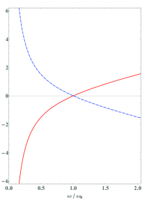
(a) $\omega_{0}\not=0$

(b) $\omega_{0}=0$

Figure 3: Eigenvalues (124) versus frequency. The vertical axis’s units are $n\omega_{0}$ (left panel) or $n\times\text{Hz}$ (right panel). Solid curves correspond to $\Lambda_{+}$, dashed ones – to $\Lambda_{-}$.

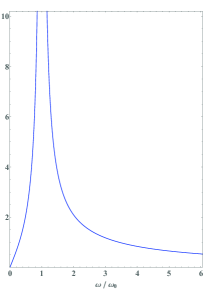
(a) $\omega_{0}\not=0$

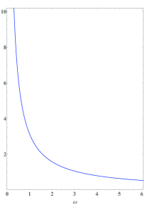
(b) $\omega_{0}=0$

Figure 4: Period of oscillations (132) versus frequency. The vertical axis’s units are $(n\omega_{0})^{-1}$ (left panel) or $(n\times\text{Hz})^{-1}$ (right panel).

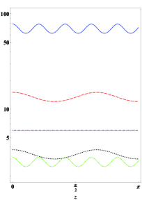
(a) $\omega_{0}\not=0$

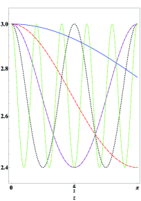
(b) $\omega_{0}=0$

Figure 5: Total energy density (135), divided by $({\cal N}_{0}/2)^{2}$, versus $z$, at $\varepsilon=\mu+1=2$ and different frequencies: $\omega/\omega_{u}=1/5$ (solid curves), $1/2$ (dashed curves), $1$ (dash-dotted curves), $2$ (dotted curves) and $5$ (dash-double-dotted curves), where $\omega_{u}$ equals to $\omega_{0}$ (left panel) or 1 Hz (right panel). The horizontal axis’s units are $h_{-}\omega_{0}$ (left panel) or $h_{-}\times\text{Hz}$ (right panel).

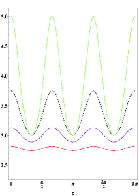
(a) $\omega_{0}\not=0$

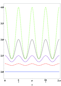
(b) $\omega_{0}=0$

Figure 6: Total energy density (135), divided by $({\cal N}_{0}/2)^{2}$, versus $z$, at $\omega/\omega_{u}=2$, $\mu=1$ and various values of relative permittivity: $\varepsilon=1$ (solid curves), $3/4$ (dashed curves), $3/2$ (dash-dotted curves), $2$ (dotted curves), and $3$ (dash-double-dotted curves), where $\omega_{u}$ equals to $\omega_{0}$ (left panel) or 1 Hz (right panel). The horizontal axis’s units are $h_{-}\omega_{0}$ (left panel) or $h_{-}\times\text{Hz}$ (right panel).

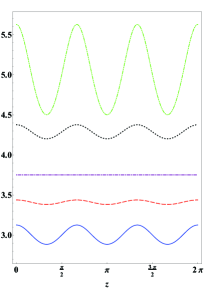
(a) $\omega_{0}\not=0$

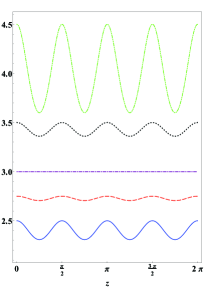
(b) $\omega_{0}=0$

Figure 7: Total energy density (135), divided by $({\cal N}_{0}/2)^{2}$, versus $z$, at $\omega/\omega_{u}=2$, $\varepsilon=3/2$ and various values of relative permeability: $\mu=1$ (solid curves), $3/4$ (dashed curves), $3/2$ (dash-dotted curves), $2$ (dotted curves), and $3$ (dash-double-dotted curves), where $\omega_{u}$ equals to $\omega_{0}$ (left panel) or 1 Hz (right panel). The horizontal axis’s units are $h_{-}\omega_{0}$ (left panel) or $h_{-}\times\text{Hz}$ (right panel).

(b) Density matrix and averages. The exact solutions of the master equations for the density operators of the system can be found in the form given by Eqs. (105) and (106), where the averages $\langle\sigma_{k}\rangle^{\prime}$ and $\langle\sigma_{k}\rangle$ satisfy Eqs. (61) and (62). The latter become, respectively,

$$\frac{1}{2}\frac{d}{dz}\begin{pmatrix}\langle\sigma_{1}\rangle^{\prime}\\ \langle\sigma_{2}\rangle^{\prime}\\ \langle\sigma_{3}\rangle^{\prime}\\ \text{tr}{\hat{\rho}^{\prime}}\end{pmatrix}=\begin{pmatrix}0&0&\lambda_{+}&\lambda_{-}\\[1.29167pt] 0&0&0&0\\[1.29167pt] -\lambda_{+}&0&0&0\\[1.29167pt] \lambda_{-}&0&0&0\end{pmatrix}\!\begin{pmatrix}\langle\sigma_{1}\rangle^{\prime}\\ \langle\sigma_{2}\rangle^{\prime}\\ \langle\sigma_{3}\rangle^{\prime}\\ \text{tr}{\hat{\rho}^{\prime}}\end{pmatrix},$$ (125)

and

$$\frac{1}{2}\frac{d}{dz}\begin{pmatrix}\langle\sigma_{1}\rangle\\ \langle\sigma_{2}\rangle\\ \langle\sigma_{3}\rangle\end{pmatrix}=\begin{pmatrix}\langle\hat{\cal G}\rangle&0&\lambda_{+}\\ 0&\langle\hat{\cal G}\rangle&0\\ -\lambda_{+}&0&\langle\hat{\cal G}\rangle\end{pmatrix}\!\begin{pmatrix}\langle\sigma_{1}\rangle\\ \langle\sigma_{2}\rangle\\ \langle\sigma_{3}\rangle\end{pmatrix}+\begin{pmatrix}\lambda_{-}\\ 0\\ 0\end{pmatrix},$$ (126)

where

$$\langle\hat{\cal G}\rangle=-\lambda_{-}\langle\sigma_{1}\rangle,$$ (127)

and $\lambda_{\pm}$ are given in Eq. (123).

As per usual, these equations must be supplemented with the “initial” (boundary) conditions (107) where for ${\hat{\rho}^{\prime}}_{0}$ we can choose either (LABEL:e:rhobloch) or (111). It turns out that the latter is suitable in this case since the corresponding normalized density matrix (112) describes the classical-type mixture of two states with equal probabilities to happen. Using Eqs. (105) and (111), we derive the following conditions for the non-normalized averages:

$$\langle\sigma_{a}\rangle^{\prime}|_{z=0}=0,\ \text{tr}{\hat{\rho}^{\prime}}|_{z=0}=2,$$ (128)

where $a=1,2,3$. Correspondingly, the solution of Eqs. (125) is

$$\langle\sigma_{1}\rangle^{\prime} = \frac{h_{-}}{n}\,\text{sin}\!\left(\beta_{z}z\right),$$ (129a)

$$\langle\sigma_{2}\rangle^{\prime} = 0,$$ (129b)

$$\langle\sigma_{3}\rangle^{\prime} = -\frac{1}{2n^{2}}F_{+}(z),$$ (129c)

$$\text{tr}{\hat{\rho}^{\prime}} = \frac{1}{2n^{2}}F_{-}(z),$$ (129d)

where

$$\beta_{z}=2n\bar{\omega},$$ (130)

and we have denoted the functions

$$F_{+}(z) = h_{+}h_{-}(1-\,\text{cos}\!\left(\beta_{z}z\right)),$$

$$F_{-}(z) = h_{+}^{2}-h_{-}^{2}\,\text{cos}\!\left(\beta_{z}z\right),$$

where the former is non-negative at $\varepsilon\geqslant\mu\geqslant 1$, and the latter is always positive for the materials with positive permittivity and permeability. This solution indicates a presence of a stationary wave, therefore it contains interference terms described by the linear combinations of sine or cosine functions.

Consequently, the normalized expectation values are

$$\langle\sigma_{1}\rangle = 2nh_{-}\,\text{sin}\!\left(\beta_{z}z\right)/F_{-}(z),$$ (131a)

$$\langle\sigma_{2}\rangle = 0,$$ (131b)

$$\langle\sigma_{3}\rangle = -F_{+}(z)/F_{-}(z).$$ (131c)

It is clear from these expressions that our statistical ensemble of wave modes has a periodic structure along $z$-direction, with the period equal to

$$T_{z}=2\pi/|\beta_{z}|=\pi/(n|\bar{\omega}|),$$ (132)

so its behavior strongly depends on the wave frequency $\omega$, see Fig. 4. When $\omega\not=0$ the dependence on $z$ can still disappear – when $\beta_{z}\to 0$, which is equivalent to $\omega\to\omega_{0}$. Thus, $\omega_{0}$ is a critical frequency at which the oscillations of the statistical averages become suppressed.

(c) Observables: wave energy. Once we know the exact solution for density matrix, we have all the information about the probability weights of every mode that forms the beam, therefore, a number of energy-related averages, which have been defined in Sec. III.3, can be easily computed. Due to real-valued permittivity and permeability, some formulas of Sec. III.3 get simplified:

$$\overline{\cal E}_{\bot}=\frac{{\cal N}^{2}_{0}}{8\omega}\langle{\cal L}_{+}\hat{\cal D}\rangle=\frac{{\cal N}^{2}_{0}}{2}G(z),$$ (133)

$$\overline{\cal E}_{z}=\frac{{\cal N}^{2}_{0}}{8\omega}\langle{\cal L}_{-}\hat{\cal D}\rangle=\frac{{\cal N}^{2}_{0}\omega^{2}_{0}}{2\omega^{2}}G(z),$$ (134)

$$\overline{\cal E}_{\text{tot}}=\overline{\cal E}_{\bot}+\overline{\cal E}_{z}=\frac{{\cal N}^{2}_{0}}{4}\left\langle\frac{\partial}{\partial\omega}\hat{\cal D}\right\rangle$$

$$\qquad=\frac{{\cal N}^{2}_{0}}{2}\left(1+\frac{\omega_{0}^{2}}{\omega^{2}}\right)G(z),$$ (135)

$$\Xi_{\cal E}\equiv\frac{\overline{\cal E}_{z}}{\overline{\cal E}_{\bot}}=\frac{\langle{\cal L}_{-}\hat{\cal D}\rangle}{\langle{\cal L}_{+}\hat{\cal D}\rangle}=\frac{\omega^{2}_{0}}{\omega^{2}},$$ (136)

$$\Xi_{\bot}\equiv\frac{\overline{\cal E}_{\bot}}{\overline{\cal E}_{\text{tot}}}=1-\frac{\overline{\cal E}_{z}}{\overline{\cal E}_{\text{tot}}}=\left(1+\frac{\omega_{0}^{2}}{\omega^{2}}\right)^{-1},$$ (137)

where

$$G(z)=\frac{h_{+}}{4}\left(1+\frac{h_{-}}{h_{+}}\langle\sigma_{3}\rangle\right)=\frac{n^{2}h_{+}}{F_{-}(z)},$$ (138)

and

$$\overline{\cal U}_{\bot}^{(e)}={\cal N}^{2}_{0}\langle\hat{e}\rangle=\frac{{\cal N}^{2}_{0}}{2}G_{+}(z),$$ (139)

$$\overline{\cal U}_{\bot}^{(m)}={\cal N}^{2}_{0}\langle\hat{g}\rangle=\frac{{\cal N}^{2}_{0}}{2}G_{-}(z),$$ (140)

$$\Xi_{{\cal U}}=\frac{\overline{\cal U}_{\bot}^{(e)}}{\overline{\cal U}_{\bot}^{(m)}}=\frac{\mu h_{+}+\varepsilon h_{-}\,\text{cos}\!\left(\beta_{z}z\right)}{\varepsilon h_{+}-\mu h_{-}\,\text{cos}\!\left(\beta_{z}z\right)},$$ (141)

where

$$G_{\pm}(z)=1\pm\langle\sigma_{3}\rangle=1\mp\frac{F_{+}(z)}{F_{-}(z)},$$ (142)

and

$$\overline{\cal P}_{z}=\frac{{\cal N}^{2}_{0}}{4}\langle\sigma_{2}\rangle=0,$$ (143)

where the averages are given by Eqs. (131), and we have used the identity

$$\frac{\partial}{\partial\omega}\hat{\cal D}=\frac{1}{\bar{\omega}}\left(1+\frac{\omega_{0}^{2}}{\omega^{2}}\right)\hat{\cal D},$$

which can be easily derived from Eqs. (97) and (117).

From these expressions, one can immediately spot a few universal features of the system. For example, energy density (135), as well as its parts, are positive functions if medium’s permittivity and permeability are positive values. These functions are oscillatory but become constant when $\varepsilon=\mu$ or $\beta_{z}=0$. The former condition defines media in which the oscillations are suppressed, therefore, the wave propagation is similar to the one in the vacuum. The latter condition is discussed above, after Eq. (132). Further, if $\omega_{0}\to 0$ then all energy gets concentrated in the transverse part $\overline{\cal E}_{\bot}$. When $\omega_{0}\not=0$, the energy tends to move to the transverse part at large frequencies $\omega$ and to the longitudinal part $\overline{\cal E}_{z}$ at small frequencies.

The example profiles of the energy-related functions of $z$, at different values of $\varepsilon$, $\mu$ and $\omega$, are given in Figs. 5-7.

(d) Entropy. In this case, the “initial” (boundary) values of the notions of entropy, which were introduced in Sec. III.5, are:

$$\left.S_{\text{vN}}\right|_{z=0}=\ln 2,\ \left.S_{\text{NH}}\right|_{z=0}=0,$$ (144)

according to Eqs. (86), (87), (105), (106) and (128). The Gibbs-von-Neumann entropy (86) for our density matrix can be computed as (in units $k_{B}=1$):

$$S_{\text{vN}}=\ln{\!(4n^{2})}-\frac{1}{2}\text{tr}\left\{\left(\hat{I}+2nh_{-}\frac{\,\text{sin}\!\left(\beta_{z}z\right)}{F_{-}(z)}\hat{\sigma}_{1}-\frac{F_{+}(z)}{F_{-}(z)}\hat{\sigma}_{3}\right)\ln{\!\left[F_{-}(z)\hat{I}+2nh_{-}\,\text{sin}\!\left(\beta_{z}z\right)\hat{\sigma}_{1}-F_{+}(z)\hat{\sigma}_{3}\right]}\right\},$$ (145)

whereas the NH entropy (87) can be derived from the relation

$$S_{\text{NH}}=S_{\rm vN}-\ln{[F_{-}(z)]}+\ln{\!(2n^{2})},$$ (146)

which follows from Eq. (88)

The behavior of the Gibbs-von-Neumann entropy at different values of frequency $\omega$ is illustrated in Fig. 8. One can see that this entropy is oscillating between its initial value, $\ln 2$, and value $1/2$, and the period of oscillations depends on the frequency, as expected from Eq. (132). Therefore, for the case $\omega_{0}\not=0$ it suffices to consider the plots with $\omega\leqslant\omega_{0}$ since this entropy is invariant under the transformation $\tilde{\omega}\to 1/\tilde{\omega}$.

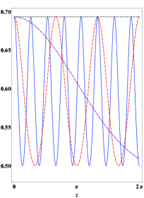
(a) $\omega_{0}\not=0$

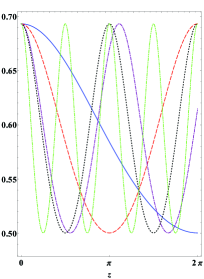
(b) $\omega_{0}=0$

Figure 8: Gibbs-von-Neumann entropy (145) versus $z$, at $\varepsilon=\mu+1=2$ and different frequencies: $\omega/\omega_{u}=1/4$ (solid curves), $1/2$ (dashed curves), $0.9$ (dash-dotted curves), $1$ (dotted curves) and $2$ (dash-double-dotted curve, right panel only), where $\omega_{u}$ equals to $\omega_{0}$ (left panel) or 1 Hz (right panel). The horizontal axis’s units are $h_{-}\omega_{0}$ (left panel) or $h_{-}\times\text{Hz}$ (right panel).

V Conclusion

In this paper, using the formal analogy between the Schrödinger equation and a certain class of Maxwell equations, we have generalized the theory of EM wave’s propagation in dielectric linear media – in order to be able to describe not only separate wave modes (or their linear superpositions) but also the statistical ensembles of modes, referred as mixed states in quantum mechanics.

It turns out that the Hamiltonians, which govern the dynamics of such ensembles, are in general not just pseudo-Hermitian but essentially non-Hermitian and thus require a special systematic treatment. Using the density operator approach for general non-Hermitian Hamiltonians developed in our earlier works, we have demonstrated that the non-Hermitian terms play an important role in the physics of wave propagation.

The proposed approach applies to a large class of dielectric media and nanoscale photonic and plasmonic materials and wave-guiding devices, where it provides a tool to construct and study different models, as well as to derive the observables of different kinds: correlation functions (Sec. III.4), entropy (Sec. III.5), energy density and transmitted power (Sec. III.3), etc. For instance, the introduced notions of entropy are important for estimating the degree of statistical uncertainty and chaos in a given system, whereas the statistically averaged values of energy density and transmitted power are helpful for describing the dissipative effects in the system due to interaction of different modes, which lead to energy and information loss. The method sheds light upon various quantum-statistical effects that can occur, such as the additional corrections to the conservation equation for the transmitted power, which arise due to the quantum exchange of energy between the medium and electric and magnetic components of wave modes, see Sec. III.3. Another effect, demonstrated by one of our examples, in Sec. IV.2, reveals that quantum-statistical corrections can make the wave’s propagation essentially dispersive, even if the media itself has frequency-independent permittivity and permeability. That example also demonstrates that non-Hermitian terms in Hamiltonians do not always lead to energy loss but can describe, under certain conditions, the oscillating behavior of statistical uncertainty in the system which can be related to certain kinds of noise.

This results in a consistent and thorough understanding of whether and how one can control the dissipative effects in different dielectric media, which lead to decoherence and energy and information loss during propagation of EM waves. The control over these effects is especially important for the development of the next generation of quantum electromagnetic devices, including those which use the quantum interference of multimode EM beams in order to improve the sensitivity and non-invasivity of measurements, quantum amplifiers and radars being just some examples cvk99 ; gat00 ; llo08 ; tan08 ; lop13 ; bar15 . For instance, the uncontrolled spontaneous transition of pure modes into statistical ensembles during beam’s propagation would inevitably result in an increase of statistical uncertainty and hence lead to higher degrees of dissipation and noise. Further studies of such quantum-statistical effects is a fruitful direction of future research.

Last but not least, one can use this approach both ways: it also provides a methodology of how one can use electromagnetic phenomena for experimental testing of the heuristic concepts and ideas of the non-Hermitian formalism per se, such as non-normalized and normalized density operators, master equations with anti-commutators, nonlinear and nonlocal terms, different notions of entropy, to mention just a few examples.

Appendix A Operator algebra and observables for EM wave modes

In case of a two-dimensional transverse space, one can define the SU(2) algebra by using the vector product with the basis vector along the longitudinal direction, $\mathbf{e}_{z}$. Indeed, when applied to a 2D vector, the operator $\mathbf{e}_{z}\times$ acts as the imaginary unit,

$$\left(\mathbf{e}_{z}\times\right)^{\dagger}=-\mathbf{e}_{z}\times,\ \ \mathbf{e}_{z}\times\mathbf{e}_{z}\times=-\hat{I},$$ (147)

which means that it is anti-Hermitian, anti-involutary and anti-unitary operator in the space of two-dimensional vectors. Therefore, using this operator one can define the following set of Pauli matrices

$$\hat{\sigma}_{1}=-i\begin{pmatrix}0&\mathbf{e}_{z}\times\\ \mathbf{e}_{z}\times&0\end{pmatrix},$$ (148a)

$$\hat{\sigma}_{2}=\begin{pmatrix}0&-\mathbf{e}_{z}\times\\ \mathbf{e}_{z}\times&0\end{pmatrix},$$ (148b)

$$\hat{\sigma}_{3}=\begin{pmatrix}\hat{I}&0\\ 0&-\hat{I}\end{pmatrix},$$ (148c)

which are Hermitian, involutary, unitary, traceless, of a unit determinant, and satisfy the commutation relations

$$\left\{\hat{\sigma}_{a},\hat{\sigma}_{b}\right\}=2\delta_{ab}\hat{I},$$ (149)

$$\left[\hat{\sigma}_{a},\hat{\sigma}_{b}\right]=2i\sum\limits^{3}_{c=1}\epsilon_{abc}\hat{\sigma}_{c},$$ (150)

where $\delta_{ab}$ and $\epsilon_{abc}$ are the Kronecker and Levi-Civita symbols, respectively. Besides,

$$\hat{\sigma}_{a}\hat{\sigma}_{b}=i\sum\limits^{3}_{c=1}\epsilon_{abc}\hat{\sigma}_{c}+\delta_{ab}\hat{\cal I},$$ (151)

$$\hat{\sigma}_{1}^{2}=\hat{\sigma}_{2}^{2}=\hat{\sigma}_{3}^{2}=-i\hat{\sigma}_{1}\hat{\sigma}_{2}\hat{\sigma}_{3}=\hat{\cal{I}}=\begin{pmatrix}\hat{I}&~{}0\\ 0&~{}\hat{I}\end{pmatrix}.~{}~{}~{}$$ (152)

The expectation values of these Pauli matrices,

$$\left\langle\sigma_{a}\right\rangle_{\Psi}\equiv\left\langle\Psi|\hat{\sigma}_{a}|\Psi\right\rangle,$$ (153)

have a physical interpretation in terms of energies associated with the EM wave: using (9) and (10) one obtains

$$\left\langle\sigma_{1}\right\rangle_{\Psi} = \frac{i}{{\cal N}^{2}}\int dxdy\left[(\mathbf{e}_{z}\times\mathbf{E}_{\bot}^{*})\cdot\mathbf{H}_{\bot}-\text{c.c.}\right]$$ (154a)

$$= \frac{i}{{\cal N}^{2}}\int dxdy\left(E^{*}_{[x}H_{y]}-\text{c.c.}\right),$$

$$\left\langle\sigma_{2}\right\rangle_{\Psi} = \frac{1}{{\cal N}^{2}}\int dxdy\left[(\mathbf{e}_{z}\times\mathbf{E}_{\bot}^{*})\cdot\mathbf{H}_{\bot}+\text{c.c.}\right]$$ (154b)

$$= \frac{1}{{\cal N}^{2}}\int dxdy\left(E^{*}_{[x}H_{y]}+\text{c.c.}\right)=\frac{4{\cal P}_{z}}{{\cal N}^{2}},~{}~{}~{}$$

$$\left\langle\sigma_{3}\right\rangle_{\Psi} = \frac{1}{{\cal N}^{2}}\int dxdy\left(|\mathbf{E}_{\bot}|^{2}-|\mathbf{H}_{\bot}|^{2}\right),$$ (154c)

where the integrals are taken over waveguide’s effective cross-section, and we use the notation $A_{[j}B_{m]}=A_{j}B_{m}-A_{m}B_{j}$. Here ${\cal P}_{z}$ is the transmitted power carried by an EM wave mode. One can also borrow the notations from theory of two-level systems and introduce the operators

$$\hat{g}\equiv\left|g\right\rangle\!\left\langle g\right|\equiv\frac{1}{2}\left(\hat{\cal{I}}-\hat{\sigma}_{3}\right)=\begin{pmatrix}0&~{}0\\ 0&~{}\hat{I}\end{pmatrix},$$ (155a)

$$\hat{e}\equiv\left|e\right\rangle\!\left\langle e\right|\equiv\frac{1}{2}\left(\hat{\cal{I}}+\hat{\sigma}_{3}\right)=\begin{pmatrix}\hat{I}&~{}0\\ 0&~{}0\end{pmatrix},$$ (155b)

where

$$\left|g\right\rangle\equiv\begin{pmatrix}0\\ \hat{I}\end{pmatrix},\ \left|e\right\rangle\equiv\begin{pmatrix}\hat{I}\\ 0\end{pmatrix},$$ (156)

such that

$$\left\langle\hat{g}\right\rangle_{\Psi}=\frac{1}{{\cal N}^{2}}\int dxdy|\mathbf{H}_{\bot}|^{2},$$ (157a)

$$\left\langle\hat{e}\right\rangle_{\Psi}=1-\left\langle\hat{g}\right\rangle_{\Psi}=\frac{1}{{\cal N}^{2}}\int dxdy|\mathbf{E}_{\bot}|^{2},$$ (157b)

where letters $g$ and $e$ indicate the “ground” and “excited” states, respectively. From the viewpoint of electrodynamics, the ratio

$$\left\langle\hat{e}\right\rangle_{\Psi}/\left\langle\hat{g}\right\rangle_{\Psi}=\left[\frac{1}{\left\langle\hat{e}\right\rangle_{\Psi}}-1\right]^{-1}$$ (158)

describes how much of wave’s “pure” energy (in absence of a medium) would be stored in the electric component as compared to the magnetic one.

Appendix B Bloch-sphere parametrization for EM wave modes

Any Hermitian operator $\hat{\varrho}$, which has trace one and idempotency property $\hat{\varrho}^{2}=\hat{\varrho}$, can be parametrized using the Bloch sphere:

$$\hat{\varrho} = \left|\Psi_{0}\right\rangle\!\left\langle\Psi_{0}\right|=\begin{pmatrix}\,\text{sin}^{2}\!\left(\theta_{0}/2\right)&\frac{1}{2}\text{e}^{i\phi_{0}}\sin\theta_{0}\\ \frac{1}{2}\text{e}^{-i\phi_{0}}\sin\theta_{0}&\,\text{cos}^{2}\!\left(\theta_{0}/2\right)\end{pmatrix}$$

$$= \frac{1}{2}\left[\hat{I}+\sin{\theta_{0}}(\cos{\phi_{0}}\,\hat{\sigma}_{1}-\sin{\phi_{0}}\,\hat{\sigma}_{2})-\cos{\theta_{0}}\hat{\sigma}_{3}\right],$$

where

$$\left|\Psi_{0}\right\rangle=\cos{(\theta_{0}/2)}\left|g\right\rangle+\text{e}^{i\phi_{0}}\sin{(\theta_{0}/2)}\left|e\right\rangle,$$ (160)

$$\left|g\right\rangle=\begin{pmatrix}0\\ 1\end{pmatrix},\ \ \left|e\right\rangle=\begin{pmatrix}1\\ 0\end{pmatrix},$$ (161)

and $0\leqslant\theta_{0}\leqslant\pi$ and $0\leqslant\phi_{0}<2\pi$. Matrix (LABEL:e:a-rhobloch) has the eigenvalues $0$ and $1$, therefore, one of its special cases would be the basis states

$$\begin{array}[]{ll}\left\{\theta_{0}=\pi,\ \phi_{0}=0\right\}:&\hat{\varrho}^{(e)}=\begin{pmatrix}1&0\\ 0&0\end{pmatrix}=\hat{e},\\ \left\{\theta_{0}=0,\ \phi_{0}=0\right\}:&\hat{\varrho}^{(m)}=\begin{pmatrix}0&0\\ 0&1\end{pmatrix}=\hat{g},\end{array}$$ (162)

where

$$\hat{g}\equiv\left|g\right\rangle\!\left\langle g\right|\equiv\frac{1}{2}\left(\hat{I}-\hat{\sigma}_{3}\right),$$ (163a)

$$\hat{e}\equiv\left|e\right\rangle\!\left\langle e\right|\equiv\frac{1}{2}\left(\hat{I}+\hat{\sigma}_{3}\right),$$ (163b)

which physical meaning is clear from Appendix A and Eqs. (73) and (74): matrices $\hat{\varrho}^{(e)}$ and $\hat{\varrho}^{(m)}$ describe the states during wave’s propagation when the wave’s “medium-independent” energy (as if the medium were absent) is stored mostly inside the electrical and magnetic field components, respectively. Consequently, we have

$$\left\langle\hat{\varrho}^{(e)}\right\rangle_{\Psi}=1-\left\langle\hat{\varrho}^{(m)}\right\rangle_{\Psi}=\frac{1}{{\cal N}^{2}}\int dxdy|\mathbf{E}_{\bot}|^{2},~{}~{}~{}$$ (164a)

$$\left\langle\hat{\varrho}^{(m)}\right\rangle_{\Psi}=\frac{1}{{\cal N}^{2}}\int dxdy|\mathbf{H}_{\bot}|^{2},$$ (164b)

where the Appendix A’s notations are used. Another example of a pure-state matrix are the following superpositions of basis states:

$$\begin{array}[]{ll}\left\{\theta_{0}=\frac{\pi}{2},\ \phi_{0}=0\right\}:&\hat{\varrho}^{(+)}=\frac{1}{2}\begin{pmatrix}1&1\\ 1&1\end{pmatrix}=|+\rangle\langle+|,\\ \left\{\theta_{0}=-\frac{\pi}{2},\ \phi_{0}=0\right\}:&\hat{\varrho}^{(-)}=\frac{1}{2}\begin{pmatrix}~{}1&-1\\ -1&~{}1\end{pmatrix}=|-\rangle\langle-|,\end{array}$$ (167)

where

$$|\pm\rangle\langle\pm| = \frac{1}{2}\left[|g\rangle\langle g|+|e\rangle\langle e|\pm\left(|g\rangle\langle e|+|e\rangle\langle g|\right)\right]$$ (168)

$$= \frac{1}{2}\left(\hat{I}\pm\hat{\sigma}_{1}\right),$$

$$|\pm\rangle = \frac{1}{\sqrt{2}}\begin{pmatrix}1\\ \pm 1\end{pmatrix}=\frac{1}{\sqrt{2}}\left(|e\rangle\pm|g\rangle\right),$$ (169)

which represent the states when the wave’s medium-independent energy is distributed between the electrical and magnetic field components, as one can see by computing the corresponding averages with respect to a state vector $|\Psi\rangle$:

$$\left\langle\hat{\varrho}^{(\pm)}\right\rangle_{\Psi}=1\pm\frac{1}{{\cal N}^{2}}\int dxdy\left(\mathbf{E}_{\bot}^{*}\cdot\mathbf{H}_{\bot}+\text{c.c.}\right).$$ (170)

References

• (1) C. C. Johnson, Field and Wave Electrodynamics (McGraw-Hill, New York, 1965).
• (2) N. S. Kapany and J. J. Burke, Optical Waveguides (Academic Press, New York and London, 1972).
• (3) R. Weder, Spectral and Scattering Theory for Wave Propagation in Perturbed Stratified Media (Springer, New York, 1991).
• (4) M. Skorobogatiy and J. Yang, Fundamentals of Photonic Crystal Guiding (Cambridge Univ. Press, New York, 2009).
• (5) A. Mostafazadeh and F. Loran, Europhys. Lett. 81, 10007 (2008).
• (6) G. Zhu, J. Lightwave Technol. 29, 905-911 (2011).
• (7) X. Yin and X. Zhang, Nature Mater. 12, 175 (2013).
• (8) L. Feng, M. Ayache, J. Huang, Y.-L. Xu, M.-H. Lu, Y.-F. Chen, Y. Fainman, and A. Scherer, Science 333, 729 (2011).
• (9) S. Longhi, Phys. Rev. Lett. 103, 123601 (2009).
• (10) S. Longhi, J. Phys. A 44, 485302 (2011).
• (11) Z. Lin, H. Ramezani, T. Eichelkraut, T. Kottos, H. Cao, and D. N. Christodoulides, Phys. Rev. Lett. 106, 213901 (2011).
• (12) L. Feng, Y.-L. Xu, W. S. Fegadolli, M.-H. Lu, J. E. B. Oliveira, V. R. Almeida, Y.-F. Chen, and A. Scherer, Nature Mater. 12, 108 (2013).
• (13) M. Kang, H.-X. Cui, T.-F. Li, J. Chen, W. Zhu, and M. Premaratne, Phys. Rev. A 89, 065801 (2014).
• (14) A. Guo, G. J. Salamo, D. Duchesne, R. Morandotti, M. Volatier-Ravat, V. Aimez, G. A. Siviloglou, and D. N. Christodoulides, Phys. Rev. Lett. 103, 093902 (2009).
• (15) K. G. Makris, R. El-Ganainy, D. N. Christodoulides, and Z. H. Musslimani, Phys. Rev. Lett. 100, 103904 (2008).
• (16) C. E. Rüter, K. G. Makris, R. El-Ganainy, D. N. Christodoulides, M. Segev, and Detlef Kip, Nature Phys. 6, 192 (2010).
• (17) A. Regensburger, C. Bersch, M.-A. Miri, G. Onishchukov, D. N. Christodoulides, and U. Peschel, Nature 488, 167 (2012).
• (18) Y. Chen, A.W. Snyder, and D. N. Payne, IEEE J. Quantum Electron. 28, 239 (1992).
• (19) A. A. Sukhorukov, Z. Xu, and Y. S. Kivshar, Phys. Rev. A 82, 043818 (2010).
• (20) A. Lupu, H. Benisty, and A. Degiron, Opt. Express 21, 21651 (2013).
• (21) Y. D. Chong, L. Ge, H. Cao, and A. D. Stone, Phys. Rev. Lett. 105, 053901 (2010).
• (22) S. Feng and K. Halterman, Phys. Rev. B 86, 165103 (2012).
• (23) Y. Sun, W. Tan, H.-Q. Li, J. Li, and H. Chen, Phys. Rev. Lett. 112, 143903 (2014).
• (24) S. Longhi, Phys. Rev. A 82, 031801 (R) (2010).
• (25) Y. D. Chong, L. Ge, and A. D. Stone, Phys. Rev. Lett. 106, 093902 (2011).
• (26) H. Alaeian and J. A. Dionne, Phys. Rev. B 89, 075136 (2014).
• (27) S. Savoia, G. Castaldi, V. Galdi, A. Alú, and N. Engheta, Phys. Rev. B 89, 085105 (2014).
• (28) R. Fleury, D. L. Sounas, and A. Alú, Phys. Rev. Lett. 113, 023903 (2014).
• (29) J. Dieudonné, Quasi-Hermitian operators, in: Proceedings of the International Symposium on Linear Spaces, Jerusalem 1960 (Pergamon, Oxford, 1961), p. 115-122.
• (30) F. G. Scholtz, H. B. Geyer and F. J. W. Hahne, Ann. Phys. 213, 74-101 (1992).
• (31) C. M. Bender and S. Boettcher, Phys. Rev. Lett. 80, 5243-5246 (1998).
• (32) F. J. Dyson, Phys. Rev. 102, 1217 (1956).
• (33) D. Janssen, F. Dönau, S. Frauendorf, and R. V. Jolos, Nucl. Phys. A 172, 145 (1971).
• (34) H.-P. Breuer and F. Petruccione, The Theory of Open Quantum Systems (Oxford Univ. Press, Oxford, 2002).
• (35) F. H. M. Faisal, Theory of Multiphoton Processes (Plenum Press, New York, 1987).
• (36) A. Sergi and K. G. Zloshchastiev, Int. J. Mod. Phys. B 27, 1350163 (2013).
• (37) K. G. Zloshchastiev and A. Sergi, J. Mod. Optics 61, 1298-1308 (2014).
• (38) A. Sergi and K. G. Zloshchastiev, Phys. Rev. A 91, 062108 (2015).
• (39) A. Sergi, Theor. Chem. Acc. 134, 79 (2015).
• (40) A. Sergi and K. G. Zloshchastiev, J. Stat. Mech. 2016, 033102 (2016).
• (41) K. G. Zloshchastiev, Eur. Phys. J. D 69, 253 (2015).
• (42) J. J. Halliwell, J. Pèrez-Mercader and W. H. Zurek (Eds.), Physical Origins of Time Asymmetry (Cambridge Univ. Press, Cambridge, 1996).
• (43) R. Loudon, The Quantum Theory of Light (Oxford Univ. Press, Oxford, 1973).
• (44) J. R. Jeffers, N. Imoto and R. Loudon, Phys. Rev. A 47, 3346-3359 (1993).
• (45) S. M. Rytov, Zh. Eksp. Teor. Fiz. 33, 166 (1957) [Soviet Phys. JETP 6, 130-140 (1958)]
• (46) G. Lindblad, Commun. Math. Phys. 48, 119-130 (1976).
• (47) C. W. Gardiner and P. Zoller, Quantum Noise (Springer, Berlin, 2000).
• (48) Anonymous referee, remark.
• (49) L. Novotny and B. Hecht, Principles of Nano-Optics (Cambridge Univ. Press, New York, 2006).
• (50) M. Cherchi, Appl. Opt. 42, 7141-7148 (2003).
• (51) S.-K. Choi, M. Vasilyev and P. Kumar, Phys. Rev. Lett. 83, 1938 (1999).
• (52) A. Gatti, E. Brambilla, L. A. Lugiato and M. Kolobov, J. Opt. B: Quantum Semiclass. Opt. 2, 196-203 (2000).
• (53) S. Lloyd, Science 321, 1463 (2008).
• (54) S.-H. Tan, B. I. Erkmen, V. Giovannetti, S. Guha, S. Lloyd, L. Maccone, S. Pirandola and J. H. Shapiro, Phys. Rev. Lett. 101, 253601 (2008).
• (55) E. D. Lopaeva, I. Ruo Berchera, I. P. Degiovanni, S. Olivares, G. Brida and M. Genovese, Phys. Rev. Lett. 110, 153603 (2013).
• (56) S. Barzanjeh, S. Guha, C. Weedbrook, D. Vitali, J. H. Shapiro and S. Pirandola, Phys. Rev. Lett. 114, 080503 (2015).