Identifying space-dependent coefficients and the order of fractionality in fractional advection diffusion equation

Abstract

Tracer tests in natural porous media sometimes show abnormalities that suggest considering a fractional variant of the Advection Diffusion Equation supplemented by a time derivative of non-integer order. We are describing an inverse method for this equation: it finds the order of the fractional derivative and the coefficients that achieve minimum discrepancy between solution and tracer data. Using an adjoint equation divides the computational effort by an amount proportional to the number of freedom degrees, which becomes large when some coefficients depend on space. Method accuracy is checked on synthetical data, and applicability to actual tracer test is demonstrated.

1 Introduction

In many natural media (river flows, aquifers, soils, porous columns) solute decay seems adequately described by models accounting for immobile fluid fraction Coats ; Deans ; Baker ; Genuch ; Schumer ; Benson . Such models are equivalent to classical Advection-Dispersion Equation equipped of supplementary operator compounding time derivative and convolution. Exponential or algebraic convolution kernels yield classical or fractional Mobile/Immobile Model Coats ; Deans ; Baker ; Genuch Schumer ; Benson . Though both variants describe experimental break-through curves Schumer ; Gaudet showing non-symmetric ascending and descending slopes, they exhibit dramatically different late time behaviors. Hence, predicting the future of a contamination event requires accurate parameter identification for each candidate model. In view of such prediction, we concentrate our attention on a method adapted to data recorded during limited time (differently from Tuan ) and on the fractional MIM

$$-\partial_{x}\left(\partial_{x}p_{1}u-Vu\right)+\partial_{t}p_{2}u+\partial_{t}^{\alpha}p_{3}u={\mathcal{R}}(x,t).$$ (1)

In this equation $\partial_{t}^{\alpha}\equiv\partial_{t}I_{0,+}^{1-\alpha}$ is a derivative of order $\alpha$ related to the temporal convolution $I_{0,+}^{1-\alpha}f(t)=\frac{1}{\Gamma\left(1-\alpha\right)}\int_{0}^{t}\frac{f\left(t^{\prime}\right)}{\left(t-t^{\prime}\right)^{\alpha}}dt^{\prime}$, itself called a fractional integral Samko , where $\Gamma$ is the Euler gamma function, $\alpha$ belongs to $]0,1[$ and ${\mathcal{R}}$ is a source term. This fractional generalization Schumer ; Benson of the Advection-Dispersion Equation describes mass transport in one-dimensional media (e.g. rivers Schumer ; Haggerty or the flow geometry considered by Young ) where fluids can be temporarily immobile and retain solutes during random trapping times of infinite average: in a porous medium, $p_{1}$, $p_{2}$ and $V$ represent a dispersion coefficient, the mobile volume fluid fraction and the water flux density (or Darcy velocity). Coefficient $p_{3}$, proportional to the immobile fluid fraction, is discussed in Section 2.1.

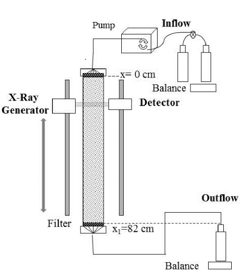
Figure 1: Di-chromatic X-ray spectrometry (DXS) device measuring water content and solute concentration at several cross-sections of a column filled of unsaturated sand. The environment of the column (mottled) achieves constant Darcy velocity $V$ and water content $\theta$, and injects tracer flux $VC_{0}$ ($V=1.05$ cm/h, $C_{0}=0.10$ mol/l) at inlet $x=0$ between time instants $0$ and $t_{f}=3$h. X ray generator and detector moved along the column measure tracer concentration and water content averaged on each desired cross-section.

We ultimately aim to check the validity of Eq. (1) for solute transport in unsaturated sand on the basis of concentration profiles recorded at several cross-sections of a column (of length $L$) filled of such a medium Latrille ; Latrille12 (see Fig.1). Some of these profiles are displayed on the left of Fig.2. However, transport properties are often sensitive to water content $\theta$ (see Gaudet ; Padilla ), measured and found steady: the right panel of Fig.2 shows that $\theta$ depends on space. Since $\theta$ may influence some coefficients of (1), we account for possible variations by linear interpolation using $n+1$ nodes including both ends of interval $[0,L]$. We do not know the most appropriate value of $n$, and try several interpolation sequences. In each attempt we estimate the best fit between data and Eq.(1) equipped of piecewise continuous coefficients. The latter are determined by their interpolation values which play the role of supplementary parameters to estimate: the right panel of Fig.2 suggests a number of nodes resulting in at least forty effective parameters. We store $\alpha$, the uniform coefficients (if there are) and the interpolation values of those which depend on space in parameter vector q which determines a solution of the discrete direct problem, namely a discrete version of Eq.(1). The smallest possible squared distance $E(\textbf{q})$ between this solution and the data gives the best candidate for q and quantifies the discrepancy between model and experiment.

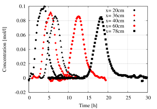
Figure 2: Solute concentration and steady water content measured in the device represented on Fig. 1. Left: solute concentration versus time, measured at some of the $15$ inspected cross sections of the column, and represented by different symbols. Right: water content $\theta$ versus position: dots and full line represent measured $\theta$ and spline interpolation with $n_{\theta}=18$ knots, less spaced in the poorly saturated region where $\theta$ exhibits stronger variations. Interpolation issued from this $n_{\theta}$ value coincides with a local average of $\theta$.

We find this minimum at the end of a sequence ($\textbf{q}_{i}$) in parameter space: each $\textbf{q}_{i+1}$ is the issue of task “ Determine $\textbf{q}_{i+1}$” in the optimization loop schematically represented on Fig.3. A robust and accurate algorithm Nocedal completes this task by deducing $\textbf{q}_{i+1}$ from $\textbf{q}_{i}$ and from the $E(\textbf{q}_{j})$ and ${\nabla}E(\textbf{q}_{j})$ issued from last and penultimate steps. Hence, action “Compute ${\nabla}E(\textbf{q})$” needs to be accurate and quick. Finite differences successively incrementing each entry of vector $\textbf{q}_{i}$ would necessitate solving at least $2n+4$ copies of the discretized p.d.e. (1) for each repetition of this task. Hence, we prefer the adjoint state method Chavent ; Chavent5 ; Sun that instead solves one adjoint equation exactly as complex as the direct discrete problem: this divides by at least $n+2$ the computing time necessary for each repetition of the loop.

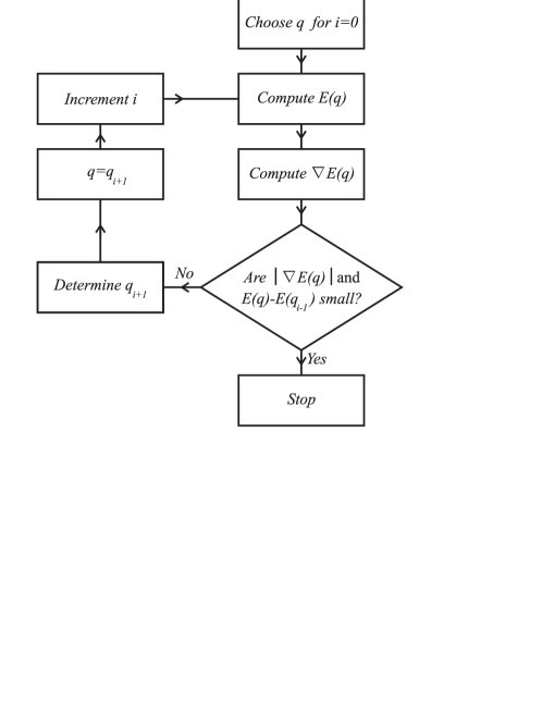
Figure 3: Principle of an optimization process minimizing $E(\textbf{q})$ by building a sequence of parameters ($\textbf{q}_{i}$). Each next element $\textbf{q}_{i+1}$ of the sequence is determined by action “Determine $\textbf{q}_{i+1}$” on the basis of inputs provided by actions “Compute $E(\textbf{q})$” and “Compute $\nabla E(\textbf{q})$” applied to $\textbf{q}_{i}$.

The fractional model (1) and the optimization problem are detailed in Section 2. Section 3 defines the adjoint equation that gives us the gradient of $E(\textbf{q})$. This sets the principle of an inversion method. A numerical experiment applied on synthetic data confirms that it accurately retrieves the coefficients of (1). Section 5 demonstrates that this approach applies to actual tracer test.

2 Mathematical model (1) and optimization problem associated with data

The time concentration profiles represented on Fig.2 were recorded in a partly saturated sand column in which the water content $\theta$ was found constant. While the Darcy velocity $V$ was also measured, $p_{1}$, $\alpha$, $p_{2}$ and $p_{3}$ could not be measured. Before estimating them by minimizing the discrepancy between the records and a numerical solution of (1) associated to boundary conditions representing the experiment, we discuss the links between measured quantities, model and parameters.

2.1 Model

The several versions of the Mobile-Immobile ModelCoats ; Deans ; Baker ; Genuch assume two fluid states (mobile and immobile) occupying volume fractions $p_{2}$ and $\theta_{im}$ of the medium. Solute concentrations are $u$ and $C_{im}$ in these two states. In water flowing through porous media, the total fluid fraction $p_{2}+\theta_{im}$ is the water content $\theta$. Dichromatic X ray Spectroscopy measures this quantity and the total solute concentration $C$ Latrille ; Latrille12 which satisfies $\theta C=p_{2}u+\theta_{im}C_{im}$. Yet, $u$, $C_{im}$, $p_{2}$ and $\theta_{im}$ are not measured.

The original version of the MIM assumes Fick’s law in mobile phase and exchanges with immobile phase obeying first order kinetic equivalent to taking $\partial_{t}C_{im}$ proportional to $u-C_{im}$. At molecular level this model is equivalent to Brownian motion interrupted during exponentially distributed time lapses Valo89 and its solutions decay exponentially at late times. Hence, a look at the tailings exhibited by the concentration records displayed on Fig.2 suggests examining the fractional variant (1) that exhibits algebraic asymptotic behavior. Nevertheless, we do not use these tailings to discriminate between the two variants because they exhibit negative records revealing large relative errors. The fractional variant is equivalent to release times distributed by stable subordinator of stability exponent $\alpha$ in $]0,1[$, an assumption that implies Schumer ; Benson

$$C=\frac{1}{\theta}\left(p_{2}{\mathrm{Id}}+p_{3}I_{0,+}^{1-\alpha}\right)u\equiv b(\theta,p_{1},p_{2},p_{3},\alpha,u),$$ (2)

where $p_{3}=\Lambda p_{2}$ also depends on $\Lambda=\lambda{\mathcal{H}}$. The latter quantity incorporates a scale factor $\lambda$ of the dimensionality of $[T]^{1-1/\alpha}$ and the probability ${\mathcal{H}}$ of being immobilized NeelZ . Fick’s law applied to the mobile concentration yields solute flux equal to

$$vp_{2}u-\partial_{x}(p_{1}u),$$ (3)

where $v$ represents a local average velocity of particles in mobile state. Inside porous columns $vp_{2}$ is commonly assumed to be equal to the Darcy velocity $V$ Sardin , a measured quantity which does not depend on $x$. Eqs.(2) and (3) imply (1) with ${\mathcal{R}}=0$.

2.2 Boundary conditions

Tracer solution of concentration $C_{0}$ injected with the fluid at flow rate $V$ at column inlet $x=0$ between time instants $t=0$ and $t_{f}$ results into tracer flux rate $VC_{0}H(t)H(t_{f}-t)$ at $x=0$, $H$ representing the Heaviside function. We assume zero diffusive flux at the outlet as Neupauer99 ; SanduG , and homogeneous initial condition meaning that the system is initially free of tracer:

$$Vu-{\partial_{x}}(p_{1}u)|_{x=0}=VC_{0}H(t)H(t_{f}-t),\quad{\partial_{x}}(p_{1}u)|_{x=L}=0,\quad u|_{t=0}=0.$$ (4)

2.3 Degrees of freedom

Water content certainly influences the mobile water content, and the right panel of Fig.2 strongly suggests that $p_{2}$ and $p_{3}$ depend on $x$. Though the inverse method presented here still works when $p_{1}$ also depends on $x$, we consider this parameter uniform for sake of simplicity and discuss this choice at the end of Section 5.2. We approximate the unknown functions $p_{2}(x)$ and $p_{3}(x)$ by linear interpolation based on $n+1$ nodes $x^{(0)}=0<x^{(1)}<...<x^{(n)}=L$ which we fix before starting parameter identification, as mentioned in the Introduction. In each interval $[x^{(i)},x^{(i+1)}]$ with $0\leq i\leq n-1$ we impose linear variations

$${p_{j}}(x)={p_{j}}^{(i)}+\frac{{p_{j}}^{(i+1)}-{p_{j}}^{(i)}}{x^{(i+1)}-x^{(i)}}\left(x-x^{(i)}\right)\>\mbox{for}\>x^{(i)}\leq x\leq x^{(i+1)}:$$ (5)

$p_{j}(x)$ depends on ${p_{j}}^{(i)}$ only if $x$ belongs to $[x^{(i-1)},x^{(i+1)}]$. Due to (5), $p_{1}$, $\alpha$ and the set of all the $p_{j}^{(i)}$ with $j=2,3$ and $i=0,...,n$ determine the solutions of problem (1-4). Therefore, we store in vector $\textbf{q}\equiv(p_{1},p_{2}^{(0)},...,p_{2}^{(n)},p_{3}^{(0)},...,p_{3}^{(n)},\alpha)^{\dagger}$ the $2n+4$ effective parameters $p_{1}$, ${p_{2}}(x^{(0)})$,…, ${p_{2}}(x^{(n)})$, ${p_{3}}(x^{(0)})$,…, ${p_{3}}(x^{(n)})$, $\alpha$ which we rename $q_{1}$, $q_{2}$,…, $q_{2n+4}$.

2.4 Discrete direct problem

In fact, only numerical approximations to the solution $u$ of problem (1-4) and to $b(\theta,p_{2},p_{3},\alpha,u)$ are available. Taking $T>t_{f}$ we specify in Appendices A.1-A.2 the approximations which we use in the space-time domain $[0,\,L]\times[0,\,T]$ discretized by $N_{Sp}+2$ space nodes $s\Delta x$ (including both ends of $[0,L]$) and $N_{T}+1$ time nodes $k\Delta t$ satisfying $L=(N_{Sp}+1)\Delta x$ and $T=N_{T}\Delta t$. The $u_{s}^{k}$ that approximate the $u\left(s\Delta x,\,k\Delta t\right)$ for $s=1,...,N_{Sp}$ and $k=0,...,N_{T}$ constitute an array noted u, of columns $\textbf{u}^{0},...,\textbf{u}^{N_{T}}$. We call $X$ the set of all arrays of $N_{Sp}$ lines and $N_{T}+1$ columns. Appendix A.2 specifies a linear algebraic problem (the discrete problem)

$$A(\textbf{q},\textbf{u})=\textbf{r}(\textbf{q}),\quad\textbf{u}\in{\mathcal{D}}(A)$$ (6)

that determines an approximation to the solution of (1-4). We call $\textbf{u}_{\textbf{q}}$ the unique array of ${\mathcal{D}}(A)\equiv\left\{\mathbf{u}\in X/\mathbf{u}^{0}=0\right\}$ solving (6) for any specified q in the convex closed set ${Q}_{\varepsilon}={R}_{+}\times[\frac{V\Delta t}{\Delta x}+\varepsilon,+\infty[^{n+1}\times{R}_{+}^{n+1}\times[0,1]$. Appendix A.3 shows that $\textbf{u}_{\textbf{q}}$ depends smoothly on q when the latter belongs to ${Q}_{\varepsilon}$.

Inside porous media, instead of $u$ we measure the total solute concentration and compare it with an approximation of $b(\theta,p_{1},p_{2},p_{3},\alpha,u)$ defined in Eq. (2).

2.5 Comparing model and data

For each $(s\Delta x,k\Delta t)$ in $]0,L[\times[0,T]$, the approximation

$$\left(B(\textbf{q},\textbf{u})\right)_{s}^{k}\equiv\frac{p_{2}}{\theta}(s\Delta x)u_{s}^{k}+\frac{p_{3}}{\theta}(s\Delta x)\sum_{j=0}^{k}{\mathcal{I}}^{j,k}u_{s}^{k-j}$$ (7)

to $b(\theta,p_{1},p_{2},p_{3},\alpha,u)(s\Delta x,k\Delta t)$ is consistent with that detailed in Appendix A.1 for $I_{0,+}^{1-\alpha}$, and we store the $\left(B(\textbf{q},\textbf{u})\right)_{s}^{k}$ in array $\textbf{B}(\textbf{q},\textbf{u})$. For $j=2,3$ this expression involves the ${p_{j}}(s\Delta x)$ which we deduce from the entries of q according to (5). The ${\mathcal{I}}^{j,k}$ are defined in Appendix A.1, and the $\theta(s\Delta x)$ are given by the spline interpolation represented at the right of Fig.2.

The total concentration $C$ is measured on ${\mathcal{N}}^{(d)}$ elements $(\bar{s}\Delta x,\,\bar{k}\Delta t)$ of the discretization grid: their indexes $(\bar{s},\bar{k})$ form the subset ${\mathcal{M}}^{(d)}$ of $\left\{1,...,N_{Sp}\right\}\times\left\{1,...,N_{T}\right\}$. We furthermore impose $\bar{k}<N_{T}$, and call $C_{\bar{s}}^{\bar{k}}$ the concentration recorded at position $\bar{s}\Delta x$ and time $\bar{k}\Delta t$. We store these records $C_{\bar{s}}^{\bar{k}}$ in an array C whose each entry of index not belonging to ${\mathcal{M}}^{(d)}$ is set equal to zero. We compare C with $\textbf{B}(\textbf{q},\textbf{u})$ by normalizing with the injected solute concentration $C_{0}$ distances issued from the standard Euclidean scalar product of $X$ (namely $\langle\textbf{u}\cdot\textbf{w}\rangle_{X}=$ $\sum_{s=1}^{N_{Sp}}\sum_{k=0}^{N_{T}}u_{s}^{k}w_{s}^{k}$ for each array w of entries $w_{s}^{k}$): we use

$$E(\textbf{q})\equiv f(\textbf{q},\,\textbf{u}_{\mathbf{q}})\equiv\sum_{{\mathcal{M}}^{(d)}}f_{\overline{s}}^{\overline{k}}\left(\textbf{q},\,\textbf{u}_{\mathbf{q}}\right),$$ (8)

to quantify the discrepancy between data and model. We have set

$$\begin{gathered}f_{\overline{s}}^{\overline{k}}\left(\textbf{q},\,\textbf{u}\right)=C_{0}^{-2}\left(\left(B\left(\textbf{q},\textbf{u}\right)\right)_{\bar{s}}^{\bar{k}}-C_{\bar{s}}^{\bar{k}}\right)^{2},\end{gathered}$$ (9)

and $\sum_{{\mathcal{M}}^{(d)}}$ stands for the complete notation $\sum_{(\bar{s},\bar{k})\in{\mathcal{M}}^{(d)}}$. Though B, $f$ and $f_{\overline{s}}^{\overline{k}}$ depend on $\theta$ and C, we do not mention these arguments.

Since array B is continuously differentiable with respect to q in $Q_{\varepsilon}$, the cost function $E$ has exactly one minimum in this closed convex set. This minimum characterizes the parameters that give to Eq. (1) the best chance of representing mass transport in the experimental conditions where the data stored in C were recorded. Robust inversion methods find such a minimum by applying rapidly converging optimization algorithms Nocedal which require gradients provided by user.

3 Cost function gradient and adjoint state

We take advantage of such algorithms provided we accurately approximate the gradient of $E$, which is significantly facilitated if we use an adjoint state.

3.1 Adjoint state

Indeed, we are searching the minimum of $f(\textbf{q},\,\textbf{u})$ when u satisfies the linear constraint (6). A standard method of constrained optimization Chavent5 consists in noticing that for each $\boldsymbol{\psi}$ in $X$ the cost function $E(\textbf{q})$ coincides with $\mathcal{L}\left(\textbf{q},\,\textbf{u}=\textbf{u}_{\textbf{q}},\,\boldsymbol{\psi}\right)$ where the functional $\mathcal{L}$ defined by

$$\mathcal{L}\left(\textbf{q},\,\textbf{u},\,\boldsymbol{\psi}\right)\equiv f(\textbf{q},\,\textbf{u})+\langle\left(A\left(\textbf{q},\,\textbf{u}\right)-\textbf{r}(\textbf{q})\right)\cdot\boldsymbol{\psi}\rangle_{X}$$ (10)

depends on the supplementary variable $\boldsymbol{\psi}$. The latter plays the role of a Lagrange multiplier: far from resulting into a more complex optimization problem, it gives us the opportunity of sparing the computation of the $2n+4$ derivatives $\frac{\partial\textbf{u}_{\textbf{q}}}{\partial q_{h}}$ in

$$\frac{\partial E}{\partial q_{h}}(\textbf{q})=\frac{\partial\mathcal{L}}{\partial q_{h}}\left(\textbf{q},\,\textbf{u}=\textbf{u}_{\textbf{q}},\,\boldsymbol{\psi}\right)+\frac{\partial\mathcal{L}}{\partial\textbf{u}}\left(\textbf{q},\,\textbf{u}=\textbf{u}_{\textbf{q}},\,\boldsymbol{\psi}\right)\left(\frac{\partial\textbf{u}_{\textbf{q}}}{\partial q_{h}}\right).$$ (11)

Indeed, a clever choice of $\boldsymbol{\psi}$ equates to zero the linear form $\frac{\partial\mathcal{L}}{\partial\textbf{u}}\left(\textbf{q},\,\textbf{u},\,\boldsymbol{\psi}\right)$ of $X$. This is easy to see upon re-writing $\frac{\partial f}{\partial\textbf{u}}\!\left(\!\textbf{q},\textbf{u}\right)(\textbf{w})$ as a scalar product $\left\langle\!\frac{\partial f}{\partial\textbf{u}}\!\left(\!\textbf{q},\textbf{u})\!\cdot\!\textbf{w}\!\right)\right\rangle_{\!X}$, so that

$$\frac{\partial\mathcal{L}}{\partial\textbf{u}}\!\left(\!\textbf{q},\textbf{u},\boldsymbol{\psi}\right)(\textbf{w})=\left\langle\!\frac{\partial f}{\partial\textbf{u}}\!\left(\!\textbf{q},\textbf{u})\!\cdot\!\textbf{w}\!\right)\right\rangle_{\!X}+\left\langle A\left(\textbf{q},\,\textbf{w}\right)\cdot\boldsymbol{\psi}\right\rangle_{X}.$$ (12)

The right hand-side of (12) in turn is viewed as a scalar product of the form $\left\langle\textbf{U}\cdot\textbf{w}\right\rangle_{X}$ with the help of operator $A^{*}$ adjoint to $A$, i.e. satisfying $\left\langle A(\mathbf{w})\cdot\mathbf{w^{\prime}}\right\rangle_{X}=\left\langle\mathbf{w}\cdot A^{*}\left(\mathbf{w^{\prime}}\right)\right\rangle_{X}$ for all $(\mathbf{w},\mathbf{w^{\prime}})$ in ${\mathcal{D}}(A)\times{\mathcal{D}}(A^{*})$. We specify $A^{*}$ and ${\mathcal{D}}(A^{*})$ in Appendix B which also shows that for any q of $Q_{\varepsilon}$ there exists one $\boldsymbol{\psi}_{\textbf{q}}$ in ${\mathcal{D}}(A^{*})$ solving

$$A^{*}(\textbf{q},{\boldsymbol{\psi}}_{\textbf{q}})=-\frac{\partial f}{\partial\textbf{u}}(\textbf{q},\textbf{u}=\textbf{u}_{\textbf{q}}),$$ (13)

called adjoint problem of (6). We easily deduce from (9) the right hand-side of (13), and solving this problem for $\boldsymbol{\psi}_{\textbf{q}}$ (the adjoint state) is no more difficult that solving the direct equation (6). Then, simple algebra using two technical points detailed in Appendix C gives us $\frac{\partial f}{\partial q_{h}}\left(\textbf{q},\,\textbf{u}=\textbf{u}_{\textbf{q}}\right)$, $\frac{\partial A}{\partial q_{h}}(\textbf{q},\textbf{u}=\textbf{u}_{\textbf{q}})$ and $\frac{\partial\textbf{r}}{\partial q_{h}}(\textbf{q})$. Thus computing the $2n+4$ components of the gradient

$$\frac{\partial E}{\partial q_{h}}({\textbf{q}})=\frac{\partial f}{\partial q_{h}}\left(\textbf{q},\,\textbf{u}=\textbf{u}_{\textbf{q}}\right)+\left\langle\left(\frac{\partial A}{\partial q_{h}}(\textbf{q},\textbf{u}=\textbf{u}_{\textbf{q}})-\frac{\partial\textbf{r}}{\partial q_{h}}(\textbf{q})\right)\cdot\boldsymbol{\psi}_{\textbf{q}}\right\rangle.$$ (14)

spares computational time.

3.2 Speeding up the optimization loop of Fig.3

Indeed, the optimization process represented on Fig.3 finds the minimum of $E$ at the end of a sequence of iterations. Each of these needs updating $E$ and its gradient by completing tasks “Compute $E(\textbf{q})$” and “Compute $\nabla E(\textbf{q})$”. The first task solves the direct problem (6) associated with $\textbf{q}_{i}$. The second updates the gradient of $E$ in three stages : (i) the right hand-side of the adjoint problem (Eq. (13)) is deduced from q and $\textbf{u}_{\mathbf{q}}$- (ii) the adjoint problem is solved for the adjoint state $\boldsymbol{\psi}_{\textbf{q}}$- (iii) inserting $\boldsymbol{\psi}_{\textbf{q}}$ and $\textbf{u}_{\mathbf{q}}$ into Eq. (14) determines the desired gradient. Since stages (i) and (iii) are of negligible computational cost, we complete task “Compute $\nabla E(\textbf{q})$” by solving one algebraic system different from (6) but no more complex. Instead determining the $2n+4$ derivatives $\frac{\partial\textbf{u}_{\textbf{q}}}{\partial q_{h}}$ by finite differences would require solving this system $2n+4$ times. Therefore, using $\boldsymbol{\psi}_{\textbf{q}}$ and (14) a priori divides the computing time by at least $n+2$. In fact, we will see in Section 4.2 that finite differences also waste accuracy, not only time.

4 Inverse method

The loop of Fig.3 gives us a parameter identification tool for Eq.(1): updating the gradient of $E$ by adjoint state method rapidly gives us the accurate information needed by efficient optimization algorithms satisfying robustness principles described below. We validate the method in a numerical experiment which also discusses practical details as tolerance values and interpolation nodes.

4.1 An algorithm that steps the $\textbf{q}_{i}$ sequence

Several strategies build $\textbf{q}_{i}$ sequences that decrease $E(\mathbf{q}_{i})$ to the minimum of the smooth function $E(\textbf{q})$ Nocedal and avoid trapping in locally flat regions. Among them, efficient quasi-Newton methods determine for $\textbf{q}_{i+1}-\mathbf{q}_{i}$ a direction pointing to the minimum of a convex quadratic local approximation ${\mathcal{E}}_{i+1}$ to $E$, updated at each step to account for the curvature of $E$ observed at most recent step. The modulus of $\textbf{q}_{i+1}-\mathbf{q}_{i}$ moreover must decrease $E$ without being too short. The BFGS (Broyden-Fletcher-Goldfarb-Shanno) formula Nocedal determines $\textbf{q}_{i+1}-\mathbf{q}_{i}$ according to these principles. It requires the gradient of $E$ at current and previous steps, but converges super-linearly to the minimum of the smooth function $E$. The L-BFGS-B free software Byrd satisfies these requirements, accounts for inequality constraints (as the definition of $Q_{\varepsilon}$), and has a limited memory version very useful in problems with many degrees of freedom as here.

Iteratively completing the three tasks represented on Fig.3 retrieves independent of $x$ parameters arbitrarily imposed to numerical solutions of (6), with relative error smaller than $0.3\%$ Maryshev13 . Because using adjoint state in action “Compute $\nabla E(\mathbf{q})$” generates economies proportional to the number of freedom degrees, this approach is expected more useful when some parameters depend on space. We specify the stopping criterion of Fig.3 and check the method efficiency by applying it on artificial data solving problem (6), and for which we know the actual value of parameter vector $\mathbf{q}$.

4.2 Validation, tolerance and interpolation nodes

We construct such data by solving the discrete direct problem (6) associated to arbitrary functions $p_{j,true}(x)$ for $j=2,3$ and numbers $p_{1,true}$ and $\alpha_{true}$. Function $\theta(x)$ is also arbitrarily chosen. In the example discussed immediately below, $\theta(x)=0.2\times(1+x/L)$, $\alpha_{true}=0.7$ and $p_{1,true}=10^{-2}$ cm²/h. The piecewise linear functions $p_{2,true}$ and $p_{3,true}$ are represented by black dashed lines at the right of Figures 4 and 5. We store $p_{1,true}$, the interpolation values of $p_{2,true}$ and $p_{3,true}$ and $\alpha_{true}$ in parameter vector $\mathbf{q}_{true}$. Then, inserting in Eq.(7) the solution of Eq.(6) gives us time profiles of $\textbf{B}(\mathbf{q}_{true},\mathbf{u}_{\mathbf{q}_{true}})$. For three values of $x$, this quantity is represented by three black dashed lines on all graphs at the left of Figures 4 and 5. These profiles play the role of the data $\mathbf{C}$ that define the objective function $E$ in Eqs.(8-9). We imagine that we do not know the true parameters and estimate them by applying to $\mathbf{C}$ the optimization process described in Section 4.1. But before, we must choose the $n+1$ interpolation nodes. This determines the dimension of $Q_{\epsilon}$. We fix the nodes by trial and error, beginning with small $n$. With the very simple functions $p_{2,true}$ and $p_{3,true}$ of Figs. 4-5, $n=4$ is sufficient. However, more complex coefficients need larger values.

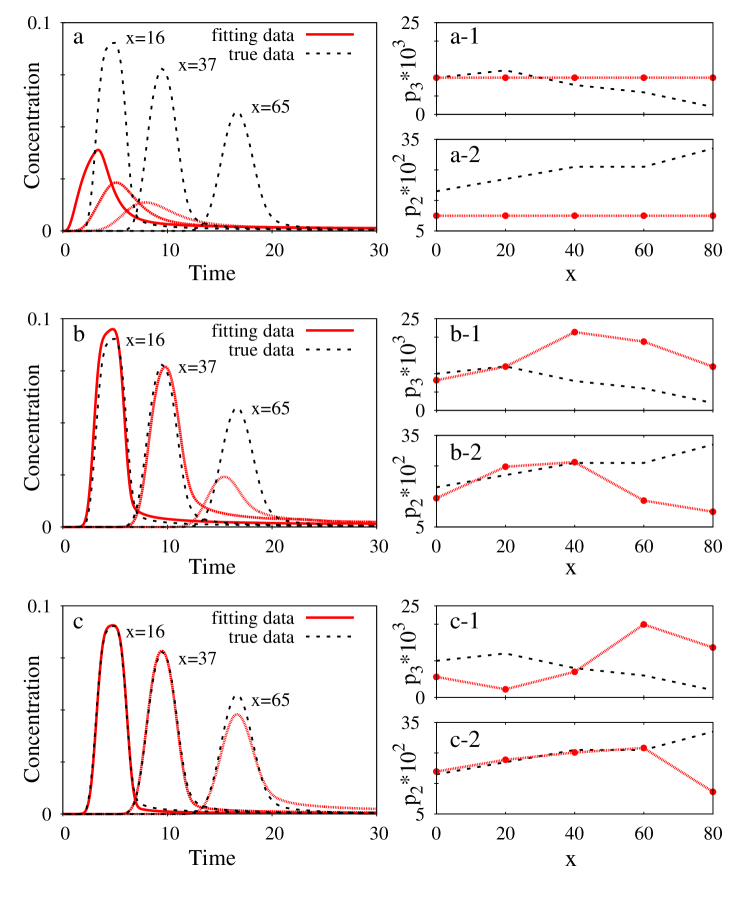
Figure 4: Profiles and estimated space dependent coefficients of Eq.(1) at some steps $i$ of the optimization applied to synthetic data. Left: total concentrations. Right: functions $p_{2}$ and $p_{3}$. Functions $p_{2,true}$ and $p_{3,true}$ and synthetic data are in black dashed lines. Estimated total concentration profiles extracted from $B({\mathbf{q}}_{i},\textbf{u}_{{\mathbf{q}}_{i}})$ and tentative estimates of $p_{2}(x)$ and $p_{3}(x)$ deduced from ${\mathbf{q}}_{i}$ are in red full lines. Step number $i$ is documented in Table 1.

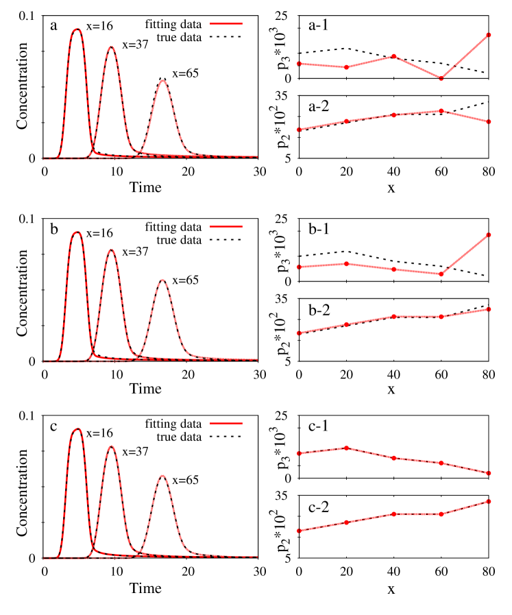
Figure 5: Profiles and estimated coefficients of (1) at several steps of the optimization applied to synthetic data, continued. Optimization is stopped at step ($i_{f}=1100$) represented on c.

For each of these choices we fix $\mathbf{q}_{0}$ at random, and stop the sequence when $E({\mathbf{q}_{i}})$ becomes stationary provided $|\nabla E({\mathbf{q}})|$ also stabilizes without being too large. Since we know the true parameters, the numerical experiment gives us the opportunity of discussing a limit tolerance value for $|\nabla E|$ at final estimate $\mathbf{q}_{i_{f}}$ on the basis of Fig.6. We observe the decrease of $E(\mathbf{q}_{i})$ which takes almost stationary values for $i$ in $\left\{200,...,800\right\}$. Yet, they correspond to non-small values of $|\nabla E({\mathbf{q}_{i}})|$ which suggest that the true minimum of $E$ ($0$ in this case) is not observed yet. Table 1 and Figs 4-5 confirm that the corresponding $\mathbf{q}_{i}$ are poor estimates of $\mathbf{q}_{true}$: tolerance values of $|\nabla E({\mathbf{q}})|$ above $10^{-1}$ are too large for the problem at hand. Yet there is no general rule, and we are ready to try tolerance values as small as possible. In fact, continuing the numerical experiment further does not improve the estimate.

plot	Fig. 4a	Fig. 4b	Fig. 4c	Fig. 5a	Fig. 5b	Fig. 5c
$p_{1},cm^{2}/h$	$3$	$2\times 10^{-7}$	$0.0206$	$0.0223$	$0.0228$	$0.0102$
$\alpha$	$0.5$	$0.529$	$0.532$	$0.53$	$0.547$	$0.697$
$E({\mathbf{q}}_{i})$	$70$	$8.4$	$0.54$	$6\times 10^{-2}$	$10^{-2}$	$10^{-5}$
Step No $i$	$0$	$10$	$40$	$140$	$400$	$1100$

Table 1: Estimated space independent parameters and cost function at some steps of optimization process applied to artificial data represented on Figures 4 and 5. Estimates documented in the table correspond to optimization steps represented on the figures.

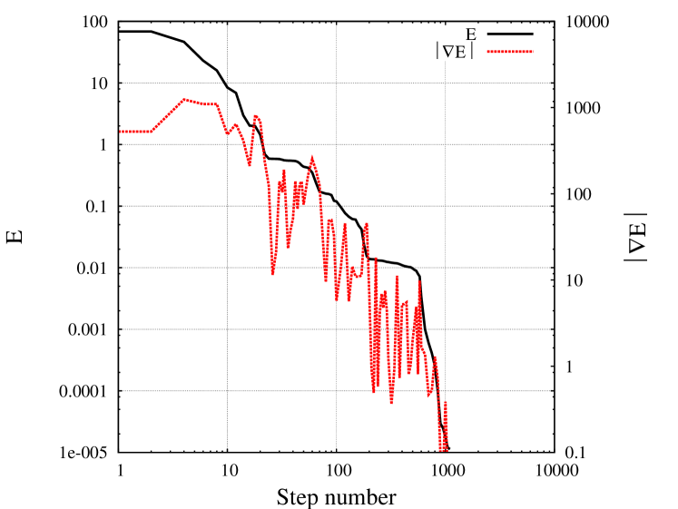
Figure 6: Cost function $E({\mathbf{q}}_{i})$ and the modulus of its gradient along the optimization procedure applied to the synthetic data represented on Figs 4-5. The $E({\mathbf{q}}_{i})$ sequence exhibits subsets where it varies slowly, but this is because the $\mathbf{q}_{i}$ sequence itself steps slowly: the too large gradient reveals that $E({\mathbf{q}})$ is far from stationary there. Continuing the process in such case is justified a posteriori by Table 1 and Fig.5.

We also tried to conduct the numerical experiment with $\nabla E(\mathbf{q})$ computed by finite differences instead of adjoint state. Approximate gradients of $E$ deduced from (14) coincide with finite difference $\frac{E(\mathbf{q}+\delta\mathbf{q})-E(\mathbf{q})}{|\delta\mathbf{q}|}$ of small enough increments $\delta\mathbf{q}$ Chavent5 . Numerical comparisons Maryshev13 confirm that for each $\eta>0$ and each $h=1,...,2n+4$ there exists $\eta^{\prime}(\eta,\mathbf{q},h)$ such that $|\delta\mathbf{q}|<\eta^{\prime}$ implies $|\frac{\partial E(\mathbf{q})}{\partial q_{h}}-\frac{E(\mathbf{q}+\delta\mathbf{q})-E(\mathbf{q})}{|\delta\mathbf{q}|}|<\eta$ when vector $\delta\mathbf{q}$ has all its entries equal to zero except that of rank $h$. Nevertheless, $\eta^{\prime}$ depends on $\mathbf{q}$: we cannot guarantee any general $\eta^{\prime}$ valid during the entire optimization process. Therefore, accurately computing gradients with finite differences needs too many checks to confirm accuracy. Implementing these checks in an automatic process is too heavy, and forgetting them returns too poor accuracy. We experienced this by running the numerical experiment with gradient deduced from finite differences of very small but fixed value. For some $\mathbf{q}$ this $|\delta\mathbf{q}|$ was not small enough and the gradient was not accurate. This resulted into extremely poor final value of $E$ (of $0.1$ compared with the better result $10^{-5}$ of Table 1) after sixty hours (four with adjoint state).

These arguments predict that adjoint state method will be even more useful with actual experimental data associated to parameters strongly suspected to vary in space.

5 Inverting actual experimental data

Actual experimental data require preliminary processing and technical choices.

5.1 Technical preliminaries

The left panel of Fig.2 displays some of the $15$ total concentration profiles recorded by DXS in the device of Fig.1. The $15$ profiles collect an amount of $3218$ triples $(x,t,C(x,t))$ among which ${\mathcal{N}}^{(n)}=357$ exhibit negative $C(x,t)$ records revealing measurement errors. We exclude from set ${\mathcal{M}}^{(d)}$ the indexes of all items that are negative or observed after negative records in descending slope (or before negative records in ascending slope). It then remains ${\mathcal{N}}^{(d)}=2861$ non-zero elements in the array C that defines $E$ in (8-9).

Before processing these data, we fix the numerical mesh and the details of the interpolation of $\theta$, $p_{2}$ and $p_{3}$. Space-time step lengths $\Delta x$ and $\Delta t$ common to discrete problems (6) and (13) are fixed according to the order of magnitude suggested by Appendix A.4 for $N_{Sp}$, taking care that the lower limit $V\frac{\Delta t}{\Delta x}$ of $p_{2}$ in the definition of $Q_{\varepsilon}$ does not exclude physically relevant tentative values: with $V=1.05$ cm/h, $\Delta x=0.25cm$ and $\Delta t=6\times 10^{-3}h$ exclude $p_{2}$ values smaller than $0.05$, i.e smaller than useful values. A posteriori comparisons to histograms of random walks Schumer ; Benson ; NeelZ approaching the solutions of (1) as in Ouloin confirm that these step lengths are small enough. In addition to the choice of the $n$ base points for the interpolation of $p_{2}$ and $p_{3}$ discussed in Section 4.2, we also interpolate the measured water content $\theta$ because of the high dispersion observed on this quantity. We use cubic splines with $n_{\theta}$ base points, taking care that interpolation coincides with local averages. Proceeding by trial and error, we progressively increase $n_{\theta}$ and $n$. The agreement between $B({\mathbf{q}},\textbf{u}_{{\mathbf{q}}})$ and the data represented on Fig.7 is achieved with $n_{\theta}=18$ and $n=31$ nodes, less spaced in the first half of the column (where they are $21$) than for $x$ between $40cm$ and $80cm$.

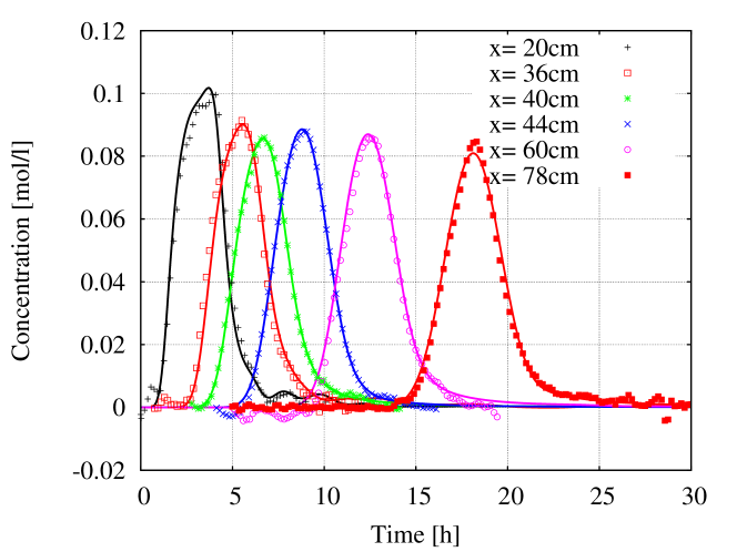
Figure 7: Total concentration, measured or deduced from $B({\mathbf{q}}_{i_{f}},\textbf{u}_{{\mathbf{q}}_{i_{f}}})$. Dots and lines represent experimental data and $B({\mathbf{q}}_{i_{f}},\textbf{u}_{{\mathbf{q}}_{i_{f}}})$. Fitted values of parameters assumed independent of $x$ are $p_{1}=3.5\times 10^{-3}$ cm²/h, $\alpha=0.89$. The estimated mobile water content profile $p_{2}\left(x\right)$ is represented on Fig. 8.

5.2 Calibration of experimental data

Each of these choices determines one minimizing sequence which follows its course automatically according to Fig.3, and we stop it at step $i_{f}$ when the $E({\mathbf{q}}_{i})$ sequence ceases moving provided the gradient of $E$ satisfies $|\nabla E({\mathbf{q}}_{i})|<10^{-1}$ as suggested in Section 4.2. Estimates of $\alpha$ and $p_{1}$ then are $0.90$ and $3.5\times 10^{-3}cm^{2}/h$, and normalized relative error

$$e_{\!R}\!=\!\frac{C_{0}\sqrt{E({\mathbf{q}}_{i_{f}})}}{\sum_{\bar{s},\bar{k}}C(\bar{s}\Delta x,\bar{k}\Delta t)}\!\approx\!2\times 10^{-3}$$

is about one order of magnitude larger than with artificial data (in Section 4.2). The averaged absolute deviation from the data is

$$e_{A}=C_{0}\sqrt{\frac{E({\mathbf{q}}_{i_{f}})}{{\mathcal{N}}^{(d)}}}=3.4\times 10^{-3}mol/l.$$

It is about $3$ times the measurement error lower bound $\sqrt{\frac{\sum_{{\mathcal{M}}^{(n)}}C(x,t)^{2}}{{\mathcal{N}}^{(n)}}}=1.4\times 10^{-3}mol/l$ suggested by the negative concentration records excluded from array $\mathbf{C}$ in section 5.1, set ${\mathcal{M}}^{(n)}$ representing the corresponding indexes. Observing the same magnitude order for $e_{A}$ and measurement error lower bound suggests that the here considered data are not badly represented by Eq. (1), here associated with small but non-negligible trapping time heterogeneity manifested by the estimate of $\alpha$.

The estimated value of $p_{1}$ suggests that we use a finite difference scheme flawed by numerical diffusion. Hence, we compared $B({\mathbf{q}}_{i_{f}},\textbf{u}_{{\mathbf{q}}_{i_{f}}})$ with the issue of the smart version of the discrete direct problem briefly described at the end of Appendix A.4. Numerical dispersion is observed. Nevertheless, the discrepancy between the two schemes is negligible in comparison with $e_{\!R}$. Also remind that we assumed parameter $p_{1}$ independent of $x$. In fact, relaxing this assumption returns the same estimates because $p_{1}$ is small: we are in a regime where the solutions of (1) are sensitive to the order of magnitude of this parameter, not to its local variations.

Estimated profiles of $\theta_{m}=p_{2}$ and $\Lambda=p_{3}/p_{2}$ deduced from final ${\mathbf{q}}_{i}$ are represented on Fig.8, along with $\theta_{im}=\theta-p_{2}$. The latter and $\Lambda$ show similar slopes in agreement with the assumption that $\Lambda$ is nearly proportional to the immobile fluid mass as the mass-exchange coefficient of the standard MIM Genuch .

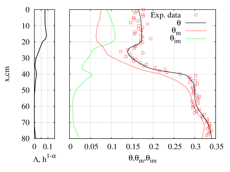
Figure 8: Profiles of space-dependent parameters $p_{2}=\theta_{m}$, $\Lambda=p_{3}/p_{2}$ and $\theta_{im}=\theta-p_{2}$. Parameters $\theta_{m}\left(x\right)$, $\theta_{im}\left(x\right)$ and $\Lambda\left(x\right)$ are estimation results, $\theta\left(x\right)$ is measured (dots) and interpolated (black line).

6 Conclusion

Adjoint states designate solutions of very diverse equations Sun ; Neupauer99 ; Maryshev13 ; Sykes ; SunYeh90 ; Neupauer04 including linear operators adjoint to the left hand-side of a p.d.e. as (1), or to a discrete formulation . The second possibility is the most efficient for parameter identification SanduG ; WilsonT minimizing the distance $E$ between data and numerical solutions to any p.d.e.

Such a minimum gives us the coefficients of Eq. (1) and the order $\alpha$ of the fractional derivative the best adapted to dispersion data composed of a series of solute concentration time profiles recorded at several locations of a medium. Heat transfer data were previously processed with a time fractional diffusion p.d.e, yet with much less degrees of freedom Ghazizadeh than here because we account for space dependent coefficients (necessitating sixty degrees of freedom).

The task is feasible though the many degrees of freedom because we do not compute the derivatives of $\textbf{u}_{\textbf{q}}$ w.r.t. the components $q_{h}$ of q, and re-formulate the cost function $E$ by introducing one adjoint state that cancels the influence of these derivatives. Instead of solving as many discrete copies of Eq.(1) as there are degrees of freedom, we determine Chavent5 this adjoint state that solves one adjoint problem of the same complexity as the direct problem that gives us $\textbf{u}_{\textbf{q}}$. This allows us varying necessary arbitrary choices which are known to strongly influence the optimization issue.

Appendix A A discrete version of the fractional MIM

Standard approximations to fractional integrals and derivatives define the discrete problem (6) whose solutions approximate those of (1).

A.1 Approximating temporal integrals and derivatives

In $p_{2}\partial_{t}+p_{3}\partial_{t}I_{0,+}^{1-\alpha}$ and in (2) the Riemann-Liouville integral $I_{0,+}^{1-\alpha}$ accounts for past history since time $t=0$. An approximation of order $O\left(\Delta t^{2}\right)$ is Diethelm

$$\begin{gathered}I_{0,+}^{1-\alpha}y(k\Delta t)\approx\sum_{j=0}^{k}{\mathcal{I}}^{j,k}y^{k-j}\quad\textrm{with}\quad{\mathcal{I}}^{0,k}={\mathcal{I}}^{0}\equiv\frac{\Delta t^{1-\alpha}}{\Gamma\left(3-\alpha\right)},\\ {\mathcal{I}}^{j,k}={\mathcal{I}}^{0}[(j+1)^{2-\alpha}-2j^{2-\alpha}+(j-1)^{2-\alpha}]\>\textmd{for}\>0<j<k,\\ {\mathcal{I}}^{0,0}=0\>\textrm{and }\>{\mathcal{I}}^{k,k}={\mathcal{I}}^{0}[(2-\alpha)k^{1-\alpha}-k^{2-\alpha}+(k-1)^{2-\alpha}]\>\textmd{ for}\>0<k.\end{gathered}$$ (15)

Combining (15) with the standard backward finite difference approximation $\frac{y^{k}-y^{k-1}}{\Delta t}$ to the first order derivative yields

$$(p_{2}\partial_{t}+p_{3}\partial_{t}I_{0,+}^{1-\alpha})y(k\Delta t)=\frac{1}{\Delta t}\sum_{j=0}^{k}W_{s}\left(j,\,k\right)y((k-j)\Delta t)+O(\Delta t),$$ (16)

with

$$\begin{gathered}W_{s}\left(0,\,k\right)=p_{2}+p_{3}{\mathcal{I}}^{0}\quad\textrm{and}\\ W_{s}\left(j,\,k\right)=p_{3}\left[{\mathcal{I}}^{j,k}-{\mathcal{I}}^{j-1,k-1}\right]+p_{2}\delta_{j,1}\>\textmd{\small for}\>1\leq j\leq k.\end{gathered}$$ (17)

A.2 Approximating spatial derivatives and boundary conditions

At each time step $k>0$ and for each $s\in\left\{1,...,N_{Sp}\right\}$, standard central finite differences

$$\frac{p_{1}}{\Delta x^{2}}\left[-\!u_{s+\!1}^{k}\!+\!\!2u_{s}^{k}-u_{s\!-\!1}^{k\!}\right]+\frac{V}{2\Delta x}\left[u_{s+\!1}^{k}\!-\!u_{s\!-\!1}^{k\!}\right],$$ (18)

approximate $-\partial_{x}\left(\partial_{x}p_{1}u-Vu\right)|_{s\Delta x}^{k\Delta t}$ at order $O(\Delta x^{2})$. Applying non-centered finite differences to the boundary conditions in (4) links $u_{0}^{k}$ and $u_{N_{Sp}+1}^{k}$ to immediately neighboring $u_{s}^{k}$, but is accurate at first order only:

$${\Delta xV+p_{1}}u_{0}^{k}={p_{1}u_{1}^{k}}+{C_{0}V}{\Delta xV+p_{1}}H(t_{f}-k\Delta t)+O(\Delta x)\>,u_{N_{Sp}+1}^{k}=u_{N_{Sp}}^{k}+O(\Delta x).$$ (19)

Hence equations (16) and (18) yield approximations to

$$-\partial_{x}\left(\partial_{x}p_{1}u-Vu\right)|_{s\Delta x}^{k\Delta t}+[(p_{2}\partial_{t}+p_{3}\partial_{t}I_{0,+}^{1-\alpha})u]|_{s\Delta x}^{k\Delta t}$$

at order $O(\Delta x)+O(\Delta t)$ for each $s\in\left\{1,...,N_{Sp}\right\}$ representing an interior point of $[0,\ell]$ and each index $k>0$. Equating them to zero and eliminating $u_{0}^{k}$ and $u_{N_{Sp}+1}^{k}$ with the help of (19) yields a system of equations determining the $u_{s}^{k}$ that approximate the $u(s\Delta x,k\Delta t)$ at interior points of $[0,\ell]$. It accounts for solute injection at column inlet. Remembering the initial condition, we set these equations in the compact form (6) reproduced below

$$A(\textbf{q},\textbf{u})=\textbf{r}(\textbf{q}),\quad\textbf{u}\in{\mathcal{D}}(A)$$

by defining linear mapping $A$ and array r. Each array u of ${\mathcal{D}}(A)\equiv\left\{\mathbf{u}\in X/\mathbf{u}^{0}=0\right\}$ satisfies the initial condition included in (4) and $A$ maps it onto array $A(\mathbf{q},{\textbf{u}})$ whose each rank $k$ column $(A(\mathbf{q},{\textbf{u}}))^{k}$ is

$$(A(\mathbf{q},{\textbf{u}}))^{k}\equiv{\textbf{G}}\textbf{u}^{k}+\sum_{j=1}^{k}\textbf{W}\left(j,\,k\right)\textbf{u}^{k-j},$$ (20)

where $\textbf{u}^{k}=(u_{1}^{k},...,u_{N_{Sp}}^{k})^{\dagger}$ represents the rank $k$ column of u. Matrices G and $\textbf{W}\left(j,\,k\right)$ are defined at the end of the section, and array r recollects the $r_{s}^{k}$ defined by

$$r_{1}^{k}=\Delta t\frac{C_{0}V}{2\Delta x}\frac{2p_{1}+V\Delta x}{V\Delta x+p_{1}}H(k\Delta t)H(t_{f}-k\Delta t),\>\>r_{s}^{k}=0\>\>\textrm{for}\>\>s>1\>\>\textrm{or}\>\>k=0.$$ (21)

Each rank $k$ column $(r_{1}^{k},...,r_{N_{Sp}}^{k})^{\dagger}$ of r being noted $\textbf{r}^{k}$, (6) is equivalent to the system of equations

$$(A(\mathbf{q},{\textbf{u}}))^{k}=\textbf{r}^{k}\quad\textrm{\small for}\quad 0\leq k\leq N_{T}.$$ (22)

With $\mu=\frac{p_{1}\Delta t}{\Delta x^{2}}$ and $\nu=\frac{V\Delta t}{2\Delta x}$, the entries $g_{s,s^{\prime}}$ of G are

$$\begin{gathered}g_{s,s^{\prime}}=0\quad\textmd{\small for}\quad|s-s^{\prime}|>1,\quad g_{s,s-1}=-\nu-\mu\quad\textmd{\small for}\quad s>1,\\ g_{s,s+1}=\nu-\mu\quad\textmd{\small for}\quad s<N_{Sp},\quad g_{s,s}=p_{2}(s\Delta x)+p_{3}(s\Delta x){\mathcal{I}}^{0}+\Omega_{s},\end{gathered}$$ (23)

where all interior diagonal entries exhibit the same $\Omega_{s}=2\mu$ (for $s\neq 1$ and $s\neq N_{Sp}$), while boundary conditions (19) result into $\Omega_{1}=\mu(1+\frac{1}{2+\mu/\nu})$ and $\Omega_{N_{Sp}}=\mu+\nu$ at both ends. We see that matrix G depends on q, $\Delta x$ and $\Delta t$. The $\textbf{W}\left(j,\,k\right)$ are $N_{Sp}\times N_{Sp}$ diagonal matrices of entries $(\textbf{W}\left(j,\,k\right))_{s,s}=W_{s}\left(j,\,k\right)$. In (20) each $\textbf{W}\left(j,\,k\right)$ operates on columns of rank smaller than $k$ stored in u.

Using (20) will help us seeing that problem (6) has exactly one solution in ${\mathcal{D}}(A)$ provided these parameters make matrix G invertible.

A.3 Well-posedness of (6)

If G is invertible, we easily determine the single solution $\mathbf{u}_{\mathbf{q}}$ of (22) in ${\mathcal{D}}(A)$ by setting ${\textbf{u}}^{0}=0$ and recursively solving equations (22), increasing $k$ from $1$ to $N_{T}$. Gershgorin circle theorem Gersh gives us a sufficient condition for matrix G invertibility in the form of

$$\left|g_{s,s}\right|>\left|g_{s-1,s}\right|(1-\delta_{s,1})+\left|g_{s+1,s}\right|(1-\delta_{s,N_{Sp}}),$$ (24)

$\delta_{i,j}$ being Kronecker index. This condition is satisfied when q belongs to any closed convex set ${Q}_{\varepsilon}={R}_{+}\times[\frac{V\Delta t}{\Delta x}+\varepsilon,+\infty[^{n+1}\times{R}_{+}^{n+1}\times[0,1]$ with $\varepsilon>0$ arbitrarily small.

By Implicit Function Theorem Jittorn the mapping $\textbf{q}\mapsto\textbf{u}_{\mathbf{q}}$ is of ${\mathcal{C}}^{\infty}$ class in $Q_{\varepsilon}$, matrices G and $\textbf{W}\left(j,\,k\right)$ having elements of class ${\mathcal{C}}^{\infty}$ in ${Q}_{\varepsilon}$ with respect to the components of q.

A.4 Numerical scheme accuracy

We validate the above scheme and fix $\Delta x$ and $\Delta t$ by considering a ${\mathcal{R}}\neq 0$ so that the continuous problem (1-4) with $C_{0}=0$ has an exact solution which we compare with the still noted $u_{s}^{k}$ issues of the above scheme. We set

$$\varphi_{0}(x)=e^{\frac{Vx}{2p_{1}}}(\sin{\sigma x}+\frac{2p_{1}\sigma}{V}\cos{\sigma x})$$

and take $\sigma$ defined by

$$\frac{2p_{1}}{V}\sigma^{2}\sin{(\sigma L)}-2\sigma\cos{(\sigma L)}-\frac{V}{2p_{1}}\sin{(\sigma L)}=0:$$

$u(x,t)\equiv t\varphi_{0}(x)$ solves (1,4) provided we set

$${\mathcal{R}}(x,t)=\varphi_{0}(x)\left[p_{2}(x)+p_{3}(x)\frac{t^{1-\alpha}}{\Gamma(2-\alpha)}+Mt\right],\quad M=p_{1}\sigma^{2}+\frac{V^{2}}{4p_{1}}.$$

Steps $\Delta x$ and $\Delta t$ must satisfy $p_{2}(s\Delta x)>\frac{V\Delta t}{\Delta x}$ to ensure $\textbf{q}\in Q_{\varepsilon}$. For instance with $L=1$, $p_{1}=0.05$, $V=1$, $\alpha=0.8$, $p_{2}(x)=0.5+0.3\sin{(4\pi x})$ and $p_{3}(x)=0.5-0.4\sin{(4\pi x)}$, taking $N_{Sp}=360$ and $\Delta t=\Delta x/10$ results into relative errors $\left|\frac{u_{s}^{k}-u(s\Delta x,k\Delta t)}{u(s\Delta x,k\Delta t)}\right|$ smaller than $2\times 10^{-4}$, for $t<1$.

This gives us an idea of which grid we can use. A posteriori checks are applied, especially when parameter identification returns large Péclet numbers. In this case the centered finite difference approximation used in Appendix A.2 for the advection term $V\partial_{x}u$ may be flawed by numerical diffusion. Hence, we compare with a modified version of the discrete direct problem (6) in which $\frac{V}{6\Delta x}(3u_{s}^{n}+u_{s-2}^{n}-6u_{s-1}^{n}+2u_{s+1}^{n})$ approximates $V\partial_{x}u$. This is Eq. (4.9) of Torrilhon which corresponds to a flux limiter given by the first line of (3.8) in this reference, in view of the small $\partial^{2}_{x^{2}}u$ which we observe. Other a posteriori checks are comparisons with random walks whose probability density function is $p_{2}u$, as in Ouloin .

Appendix B Discrete adjoint state for discrete direct problem (6)

The linear operator $A$ is described by (20), which implies

$$\left\langle A(\textbf{q},\textbf{u})\!\cdot\!\textbf{w}\right\rangle_{\!X}\!=\!\!\sum_{k=1}^{N_{T}}\!\left\langle\textbf{G}\textbf{u}^{k}\!\cdot\!\textbf{w}^{k}\right\rangle_{{R}^{N_{\!Sp}}}\!\!+\!\!\sum_{k=1}^{N_{T}}\sum_{j=1}^{k}\left\langle\textbf{W}(j,\,k)\textbf{u}^{k-j}\!\cdot\!\textbf{w}^{k}\right\rangle_{{R}^{N_{Sp}}},$$ (25)

for each $(\textbf{u},\textbf{w})$ in ${\mathcal{D}}(A)\times X$. Matrices G and $\textbf{W}(j,\,k)$ are defined in Appendix A.2, and each $\left\langle\textbf{G}\textbf{u}^{k}\!\cdot\!\textbf{w}^{k}\right\rangle_{{R}^{N_{\!Sp}}}$ is equal to $\langle\textbf{u}^{k}\cdot\textbf{G}^{\dagger}\textbf{w}^{k}\rangle_{{R}^{N_{Sp}}}$, superscript ${\dagger}$ denoting transpose. Re-arranging the double sum on the right hand-side of (25) proves that the adjoint $A^{*}$ of $A$ is the operator that transforms each array w of $X$ into array $A^{*}(\textbf{q},\textbf{w})$ whose each column of rank $k$ is

$$(A^{*}(\textbf{q},\textbf{w}))^{k}=\textbf{G}^{\dagger}\textbf{w}^{k}+\sum_{j=1}^{N_{T}-k}\textbf{W}\left(j,\,k+j\right)\textbf{w}^{k+j}\quad{\mbox{for}}\quad 0\leq k\leq N_{T}.$$ (26)

This implies that Eq.(13) is equivalent to the set of all equations

$$\textbf{G}^{\dagger}\boldsymbol{\psi}^{k}+\sum_{j=1}^{N_{T}-k}\textbf{W}\left(j,\,k+j\right)\boldsymbol{\psi}^{k+j}=-\sum_{{\mathcal{M}}^{(d)}}\left(\frac{\partial f_{\bar{s}}^{\bar{k}}}{\partial\mathbf{u}}\right)^{k}(\textbf{q},\,\textbf{u}_{\mathbf{q}})$$ (27)

obtained for $0\leq k\leq N_{T}$. When G is invertible it is the same for $\textbf{G}^{\dagger}$, hence the system of all these equations has exactly one solution in ${\mathcal{D}}(A^{*})=\left\{\textbf{u}\in X\big{/}\textbf{u}^{N_{T}}=0\right\}$ because the final simulation time $T$ is such that $\max\left\{\bar{k}\big{/}(\bar{k},\bar{s})\in{\mathcal{M}}^{(d)}\right\}<N_{T}$ which implies $\left(\frac{\partial f_{\bar{s}}^{\bar{k}}}{\partial\textbf{u}}\right)^{N_{T}}\left(\textbf{q},\textbf{u}\right)=0$, hence $\boldsymbol{\psi}^{N_{T}}=0$ because G is invertible. Then, for each $k<N_{T}$ Eq.(27) is of the form of

$$\textbf{G}^{\dagger}\boldsymbol{\psi}^{k}={\mathcal{F}}(\theta,\textbf{q},\,\textbf{u}_{\mathbf{q}},\,\textbf{C},\boldsymbol{\psi}^{k+1},...,\boldsymbol{\psi}^{N_{T}})$$

and has exactly one solution in ${R}^{N_{Sp}}$ entirely determined by $\boldsymbol{\psi}^{k+1},...,\boldsymbol{\psi}^{N_{T}}$, q, $\theta$ and C. All these $\boldsymbol{\psi}^{k}$ form the unique solution of Eq.(13) in ${\mathcal{D}}(A^{*})$, which we call $\boldsymbol{\psi}_{\textbf{q}}$.

Appendix C The derivatives of $E$ w.r.t the parameters

The adjoint problem (13) depends on the differential of $f$ w.r.t. u, and determining the gradient of $E$ w.r.t. q also needs the derivatives of $f$, $A$, and r w.r.t. the entries $q_{h}$ of q. Though standard algebra returns these derivatives, two points are worth being mentioned.

First, for $j=2,3$, the $\partial E/\partial p_{j}^{(i)}$ are obtained by applying chain rule to (14) and (5).

Then, the derivative w.r.t. $\alpha$ involves $\frac{\partial{\mathcal{I}}^{0}}{\partial\alpha}$, $\frac{\partial\left(\!{\mathcal{I}}^{j\!-\!1,k\!-\!1}\!-\!{\mathcal{I}}^{j\!-\!1,k\!-\!1}\!\right)}{\partial\alpha}$ and $\frac{\partial f_{\bar{s}}^{\bar{k}}}{\partial\alpha}$ for which we need the digamma function $\frac{\Gamma^{\prime}}{\Gamma}$ Abr

$$\frac{\Gamma^{\prime}}{\Gamma}(z+1)=\gamma\sum_{k=1}^{\infty}\frac{z}{k(z+k)},$$ (28)

where $\gamma$ is Euler constant. We obtain

$$\frac{\partial{\mathcal{I}}^{0}}{\partial\alpha}={\mathcal{I}}^{0}\left[-\ln(\Delta t)+\frac{\Gamma^{\prime}}{\Gamma}(3-\alpha)\right],$$

and

$$\begin{gathered}\frac{\partial{\mathcal{I}}^{j,k}}{\partial\alpha}={\mathcal{I}}^{0}\left[(j+1)^{2-\alpha}-2j^{2-\alpha}+(j-1)^{2-\alpha}\right]\left(-\ln(\Delta t)+\frac{\Gamma^{\prime}}{\Gamma}(3-\alpha)\right)\\ -\left[\ln(j+1)(j+1)^{2-\alpha}-2\ln(j)j^{2-\alpha}+\ln(j-1)(j-1)^{2-\alpha}\right]\quad\mbox{for}\quad 1<j<k,\\ \frac{\partial{\mathcal{I}}^{k,k}}{\partial\alpha}={\mathcal{I}}^{0}\left[(2-\alpha)k^{1-\alpha}-k^{2-\alpha}+(k-1)^{2-\alpha}\right]\left(-\ln(\Delta t)+\frac{\Gamma^{\prime}}{\Gamma}(3-\alpha)\right)\\ -\left[k^{1-\alpha}+(2-\alpha)\ln(k)k^{1-\alpha}-\ln(k)k^{2-\alpha}+\ln(k-1)(k-1)^{2-\alpha}\right].\end{gathered}$$

References

• (1) K. H. Coats, B. D. Smith, Dead-end pore volume and dispersion in porous media. Soc. Petrol. Eng. J. 4 (1) pp 73–84 (1964)
• (2) H.A. Deans, A mathematical model for dispersion in the direction of flow in porous media. Soc. Pet. Eng. J. 3, p. 49 (1963).
• (3) L.E. Baker, Effects of dispersion and dead-end pore volume in miscible flooding. Soc. Pet. Eng. J. 17, p. 319 (1977).
• (4) M. Th. van Genuchten, P. J. Wierenga, Mass Transfer Studies in Sorbing Porous Media I. Analytical Solutions. Soil. Sci. Soc. Am. J. 40 (4) pp 473–480 (1976).
• (5) R. Schumer, D. A. Benson, M. M. Meerschaert, B. Baeumer, Fractal mobile/immobile solute transport. Water Resources Res. 39 (10) p. 1296 (2003).
• (6) D. A. Benson, M. M. Meerschaert, A simple and efficient random walk solution of multi-rate mobile/immobile mass transport equations. Advances in Water Res. 32 pp 532–539 (2009).
• (7) J.P. Gaudet, H. Jégat, V. Vachaud and J.P. Wierenga Solute transfer, with exchange between mobile and stagnant water, through unsaturated sand. Soil Sci. Am. J. 41, (4), p 665 (1977).
• (8) V.K. Tuan, Inverse problem for fractional diffusion equation. Frac. Calc. Appl. Anal. 14(1) pp 31–54 (2011).
• (9) S.G. Samko, A.A . Kilbas, O.I. Marichev, Fractional integrals and derivatives: theory and applications. Gordon and Breach, New York, (1993).
• (10) R. Haggerty, S. A. McKenna, L. C. Meigs, On the late-time behavior of tracer test breakthrough curves. Water Resources Res. 36 (12) pp 3467–3479 (2000).
• (11) W.R. Young, Arrested shear dispersion and other models of anomalous diffusion. J. Fluid Mech. 193, pp 129–149 (1988).
• (12) C. Latrille, A. Cartalade, New experimental device to study transport in unsaturated porous media, Water- Rock Interaction. CRC Press, Leiden pp 299–302 (2010).
• (13) C. Latrille, M.C. Néel, Transport study in unsaturated porous media by tracer test experiment in a dichromatic X-ray experimental device. Tracer 6, Sixth International Conference in Tracers and Tracing Methods, Oslo june 2011, EPJ Web of conferences (2012).
• (14) I. Y. Padilla, T.-C. J. Yeh, M. H. Conklin, The effect of water content on solute transport in unsaturated porous media. Water Res. Res. 35 (11) pp 3303–3313 (1999).
• (15) J. Nocedal, S. J. Wright, Numerical Optimization. Springer-Verlag, Berlin, New York (1999).
• (16) G. Chavent, Identification of functional parameters in partial differential equations. in Identification of parameters in distributed systems. Proc. of the Joint Automatic Control Conference, Ed. Goodson and Polis, The American Society of Mechanical Engineers (1974).
• (17) G. Chavent, Nonlinear Least Squares for Inverse Problems. Theoretical Foundations and Step-by-Step Guide for Applications. Springer (2009).
• (18) N.-Z. Sun, Inverse Problems in Groundwater Modeling, Theory and applications of transport in porous media. Vol 6, Kluwer Academic Publishers, Dordrecht (1994).
• (19) A. Valocchi, H.A.M. Quinodoz, Groundwater Contamination. IAHS Publ., L. M. Abriola Ed. 185 pp 35-42 (1989).
• (20) M.C. Néel, A. Zoia, M. Joelson, Mass transport subject to time-dependent flow with nonuniform sorption in porous media. Phys. Rev. E (80) 05631 (2009)
• (21) M. Sardin, D. Schweich, F. J. Leu, M. Th. van Genuchten, Modeling the Nonequilibrium transport of linearly interacting solutes in porous media: a review. Water Res. Res. 27 (9) pp 2287–2307 (1991).
• (22) R. Neupauer, J. Wilson, Adjoint method for obtaining backward and travel time probabilities of a conservative groundwater contaminant. Water Resources Res. 35(11) pp 3389-3398 (1999).
• (23) T. Gou, A. Sandu, Continuous versus discrete advection adjoints in chemical data assimilation. Atm. Envi. 45 pp 4868–4881 (2011).
• (24) R. H. Byrd, P. Lu, J. Nocedal, C. Zhu, A Limited Memory Algorithm for Bound Constrained Optimization. SIAM Journal on Scientific and Statistical Computing 16 (5) pp 1190–1208 (1995).
• (25) B. Maryshev, A. Cartalade, C. Latrille, M. Joelson, M.C. Néel, Adjoint state method for fractional diffusion: parameter identification. Comput. Math. Appl. 66 pp 630-638 (2013).
• (26) M. Ouloin, B. Maryshev, M. Joelson, C. Latrille and M.C.Néel, Laplace-transform based inversion method for fractional dispersion. Transport in porous media 98 (1) pp 1-14 (2013).
• (27) M. Cada and M. Torrilhon, Compact third-order limiter functions for finite volume methods, J.C.P. 228 pp. 4118-4145 (2009).
• (28) J.F. Sykes, J.L. Wilson, R.W. Andrews, Sensitivity analysis for steady state groundwater flow using adjoint operators. Water Resources Res. 21(3) pp 359-371 (1985).
• (29) N.Z. Sun, and W.W.G. Yeh, Coupled inverse problems in groundwater modeling, 1, Sensitivity analysis and parameter identification. Water Resources Res. 26(10) pp 2507-2525 (1990).
• (30) R. Neupauer, J. Wilson, Forward and backward location probabilities for sorbing solutes in groundwater. Adv. Water Res. 27 pp 689-705 (2004).
• (31) L.R. Townley and J.L. Wilson, Computationally efficient algorithms for parameter estimation in numerical models of groundwater flow. Water Resources Res. 21(12) pp 851-1860 (1985).
• (32) H. R. Ghazizadeh, A. Azimi, M. Maerefat, An inverse problem to estimate relaxation parameter and order of fractionality in fractional single-phase-lag heat equation, Int. J. Heat Mass Transfer 55 pp 2095–2101 (2012).
• (33) A.C. Galucio, J.F. Deü, S. Mengué, F. Dubois, An adaptation of the Gear scheme for fractional derivatives. Comput Methods Appl. Mech. Engrg. 195 pp 6073–6085 (2006).
• (34) Q. Liu, F. Liu, I. Turner, V. Anh, Y.T. Gu, A RBF meshless approach for modeling fractional mobile/immobile transport model. Appli. Math. and Comput. 226 pp 336–247 (2014).
• (35) F. Liu, P. Zhuang, K. Burrage, Numerical methods and analysis for a class of fractional advection-dispersion models. Computers and Maths with Appli. 64 pp 2990–3007, (2012).
• (36) K. Diethelm, N. J. Ford, A. D. Freed, Y. Luchko, Algorithms for the fractional calculus: A selection of numerical methods, Comput Methods Appl. Mech. Engrg. 194 pp 743–773 (2005).
• (37) S. Gerschgorin, Uber die Abgrenzung der Eigenwerte einer Matrix. Izv. Akad. Nauk. USSR, Otd. Fiz.-Mat. Nauk 6 pp 749–754 (1931).
• (38) K. Jittorntrum, An Implicit Function Theorem. J. Optimization Theory and Applications 25(4) pp 575–577 (1978).
• (39) M. Abramowitz, I.A. Stegun, Handbook of mathematical functions with formulas, graphs and mathematical tables, New York, Dover, 10th ed. (1972)