Low-rank Multi-view Clustering in Third-Order Tensor Space

Abstract

The plenty information from multiple views data as well as the complementary information among different views are usually beneficial to various tasks, e.g., clustering, classification, de-noising. Multi-view subspace clustering is based on the fact that the multi-view data are generated from a latent subspace. To recover the underlying subspace structure, the success of the sparse and/or low-rank subspace clustering has been witnessed recently. Despite some state-of-the-art subspace clustering approaches can numerically handle multi-view data, by simultaneously exploring all possible pairwise correlation within views, the high order statistics is often disregarded which can only be captured by simultaneously utilizing all views. As a consequence, the clustering performance for multi-view data is compromised. To address this issue, in this paper, a novel multi-view clustering method is proposed by using t-product in third-order tensor space. Based on the circular convolution operation, multi-view data can be effectively represented by a t-linear combination with sparse and low-rank penalty using “self-expressiveness”. Our extensive experimental results on facial, object, digits image and text data demonstrate that the proposed method outperforms the state-of-the-art methods in terms of many criteria.

I Introduction

Benefitting from the advance of information technology, multiple views of objects can be readily acquired in many real-world scenarios, which include different kinds of features [32][41]. In essence, most datasets are comprised of multiple feature sets or views. For instance, an object can be characterized by a color view and/or a shape view; an image can be depicted by different features such as color histogram and Fourier shape information, etc. These multi-view data provide more useful information, compared to single-view data, to boost clustering performance by integrating different views [2, 18]. In general, multi-view clustering [2, 18, 32, 41] is superior to single-view one due to utilizing the complementary information of objects from different feature spaces.

However, a challenging problem may arise when data from different views show a large divergence, or being heterogeneous [8]. As such, it will lead to view disagreement [37] so as to fail to obtain a similarity matrix that can depict the samples within the same class. Specifically, the within-class samples across multiple views may show a lower affinity than that within the same view but from different classes [8]. In order to address this problem, a surge of methods in multi-view learning have been proposed [18, 22, 33, 36, 39, 45]. Tzortzis et. al [33] proposed to compute separate kernels on each view and then combined with a kernel-based method to improve clustering. To better capture the view-wise relationships among data, in work [36], a novel multi-view learning model has been presented via a joint structured sparsity-inducing norm. For exploiting the correlation consensus, a co-regularized multi-view spectral clustering [39] is developed by using two co-regularization schemes. Liu et. al [22] proposed a non-negative matrix factorization (NMF) based multi-view clustering algorithm via seeking for a factorization that gives compatible clustering solutions across multiple views. By taking advantage of graph Laplacian matrices [43][44] in different views, the algorithm proposed in [4] learns a common representation under the spectral clustering framework. Though the aforementioned methods indeed enhance the clustering performance for multi-view data, some useful prior information within data are often ignored, such as sparsity [9] and low-rank [21], etc. To tackle this problem, a novel pairwise sparse subspace representation model for multi-view clustering was proposed recently [45]. Ding et. al [7] developed a robust multi-view subspace learning algorithm by seeking a common low-rank linear projection to mitigate the semantic gap among different views. Xia et. al [40] presented recovering a shared low-rank transition probability matrix, in favor of low-rank and sparse decomposition, and then input to the standard Markov chain method for clustering. To further mitigate the divergence between different views, Ding et. al [8] proposed a robust multi-view subspace learning algorithm (RMSL) through dual low-rank decompositions, which is expected to recover a low-dimensional view-invariant subspace for multi-view data. In fact, this type of subspace learning approaches aims to achieve a latent subspace shared by multiple views provided the input views are drawn from this latent subspace.

In recent years, subspace clustering has attracted considerable attentions in computer vision and machine learning communities due to its capability of clustering data efficiently [34]. The underlying assumption is that observed data usually lie in/near some low-dimensional subspaces [28]. By constructing a pairwise similarity graph, data clustering can be readily transformed into a graph partition problem [31, 44, 43]. The success of subspace clustering is based on a block diagonal solution that is achieved given that the objective functions satisfy some enforced block diagonal (EBD) conditions [25]. Mathematically, the objective functions are designed as a reconstruction term with different regularization, such as, either $\ell_{1}$-minimization (SSC) [9], rank minimization (LRR) [21] or $\ell_{2}$-regularization (LSR) [25]. Although subspace learning shows good performance in multi-view clustering, they may not fully make use of the properties of multi-view data. As discussed above, most previous methods focus on capturing only the pairwise correlations between different views, rather than the higher order correlation [29] underlying the multi-view data. In fact, the real world data are ubiquitously in multi-dimension, often referred to as tensors. Based on this observation, especially for multi-view data, omitting correlations in original spatial structure cannot result in optimal clustering performance generally. To address this issue, Zhang et. al. [47] proposed a low-rank tensor constrained multi-view subspace clustering to explore the complementary information from multiple views. However, the work [47] cannot capture high order correlations well since it does not actually represent view data as a tensor.

Recently, the t-product [13], one type of tensor-tensor products, was introduced to provide a matrix-like multiplication for third-order tensors. The t-product shares many similar properties as the matrix product and it has become a better way of exploiting the intrinsic structure of third-order or higher order tensor [12], against the traditional Kronecker product operator [16]. To perform subspace clustering on data with second-order tensor structure, i.e., images and multi-view data, conventional methods usually unfold the data or map them to vectors. Thus blind vectorizing may cause the problem of “curse of dimensionality” and also damage the second-order structure, like spatial information, within data. In contrast, t-product provides a novel algebraic approach for convolution operation rather than scalar multiplication [13]. Owing to this operator, a third-order tensor can be readily regarded as a “matrix” whose elements are n-tuples or tubes, such that the matrix data can be embedded into a vector-space-like structure [12]. To exactly recover a low-rank third-order tensor corrupted by sparse errors, most recent work [24] studied the Tensor Robust Principal Component (TRPCA). To perform submodule clustering of multi-way data, Piao et. al [30] proposed a clustering method by sparse and low-rank representation using t-product. However, this method is not developed for multi-view data, which is in favor of the linear separability assumption rather than complementary information of multi-view data. In fact, it is easier to treat multi-view data as a third-order tensor by organizing all different views of an object together, referring to Section IV-A for more details.

Motivated by the above observations, we propose a novel low-rank multi-view clustering method by using t-product based-on the circular convolution in this paper. The proposed method aims to capture within-view relationships among multi-view data while respecting the feature-wise effect of each data point. By some manipulations, we can naturally transform the multiple views data of interest into a third-order tensor. In nature, the multi-view data is readily regarded as a tensor. In what follows, we can apply the recent advance of third-order tensor algebra tools [14, 15, 48] to performing clustering or classification tasks. Specifically, each sample from different views (i.e., with $D\times k$ ) can be twisted into a third-order tensor with $D\times 1\times k$ and all samples can be organized as a tensor with $D\times n\times k$. Then the tensorial data can be represented by the t-linear combination for data “self-expressiveness”. The overview of our proposed method is shown in Fig. 1.

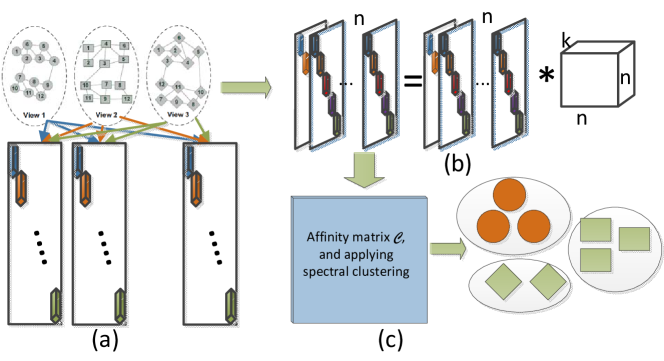
Figure 1: Overview of the proposed framework. (a) Using third-order tensorial data to represent a multi-view dataset. Each lateral slice of tensor is formed by all views from one object where each view data is arranged at the diagonal position one-by-one. (b) By t-linear combination, the third-order tensorial data is reconstructed by itself with sparse and low-rank penalty in self-expressive way. (c) Based on the learned tensor coefficients, a data similarity matrix is built for multi-views, by which the spectral clustering is applied to the final separation.

Our main contributions in this paper are summarized from the following three aspects:

1. First, we present an innovative construction method by effectively organizing multi-view data set into third-order tensorial data. As such, multiple views can be simultaneously exploited, rather than only pairwise information.

2. More importantly, to the best of our knowledge, it is the first time to propose a low-rank multi-view clustering in third-order tensor space. Through using t-product based on the circular convolution operation, the multi-view data is represented by a t-linear combination imposed by sparse and low-rank penalty using “self-expressiveness”. Therefore, the high order structural information among all views can be efficiently explored and the underlying subspace structure within data can be also revealed.

3. We perform the proposed approach on the extensive multi-view databases, such as facial, object, digits image and text data, to verify the effectiveness of the algorithm.

The remainder of this paper is organized as follows. In Section II, we introduce some notations and definitions used throughout this paper. Section III briefly reviews the related works. Section IV is dedicated to presenting the proposed multi-view clustering. In Section V, we present experimental results on evaluating clustering performance for several databases. Finally, Section VI concludes our paper.

II Notations and definitions

In this section, we would like to introduce some notations and some relevant definitions. Throughout this paper, we utilize calligraphy letters for tensors, e.g. $\mathcal{A}\in\mathbb{R}^{n_{1}\times n_{2}\times n_{3}}$, bold lowercase letters for vectors, e.g. $\mathbf{a}$, uppercase for matrices, e.g. ${A}$, lowercase letters for entries, e.g. $a$, $a_{ij}$ denotes the $(i,j)$-th entry of matrix $A$. $\|\textbf{a}\|_{1}=\sum_{i}|{a}_{i}|$ and $\|\textbf{a}\|_{2}=\sqrt{\textbf{a}^{T}\textbf{a}}$ are the $\ell_{1}$ and $\ell_{2}$ norms respectively, where ^T is the transpose operation. The matrix Frobenius norm is defined as $\left\|A\right\|_{F}=\sqrt{\sum_{ij}{{\left|{a_{ij}}\right|^{2}}}}$. $\|A\|_{*}$ is the nuclear norm, defined as the sum of all singular values of $A$, which is the convex envelope of the rank operator. $\|A\|_{2,1}$ is the $\ell_{2,1}$-norm defined by $\|A\|_{2,1}=\sum_{j}{\sqrt{\sum_{i}a_{ij}^{2}}}$.

We also use Matlab notation to denote the elements in tensors. Specifically, $\mathcal{A}(:,:,i)$, $\mathcal{A}(:,i,:)$ and $\mathcal{A}(i,:,:)$ are represented by the $i$-th frontal, lateral and horizontal slice, respectively. $\mathcal{A}(:,i,j)$, $\mathcal{A}(i,:,j)$ and $\mathcal{A}(i,j,:)$ denote the mode-1, mode-2 and mode-3 fiber, respectively. We denote $\hat{\mathcal{A}}$ the Discrete Fourier Transform (DFT) along mode-3 for a third-order tensor $\mathcal{A}$, i.e., $\hat{\mathcal{A}}=\text{fft}(\mathcal{A},[\;],3)$. Similarly, $\mathcal{A}$ can be computed by $\hat{\mathcal{A}}$ via ifft$(\hat{\mathcal{A}},[\;],3)$, i.e., using inverse fast Fourier transform (FFT). ${A}^{(i)}$ and $\hat{{A}}^{(i)}$ denote the $i$-th frontal slice of $\mathcal{A}$ and $\hat{\mathcal{A}}$, respectively. We give the following definitions, similar to those in [12].

Definition 1 (block diagonal operation (bdiag)[15]).

For $\mathcal{A}$, its block diagonal matrix is formed by its frontal slice with each block on diagonal.

$$\text{bdiag}(\mathcal{A})=\left[\begin{array}[]{cccc}{A}^{(1)}&&&\\ &{A}^{(2)}&&\\ &&\ddots&\\ &&&{A}^{(n_{3})}\\ \end{array}\right].$$ (1)

Definition 2 (block circulant operation (bcirc)).

For $\mathcal{A}$, its block diagonal matrix is defined as following.

$$\text{bcirc}(\mathcal{A})=\left[\begin{array}[]{cccc}{A}^{(1)}&{A}^{(n_{3})}&\cdots&{A}^{(2)}\\ {A}^{(2)}&{A}^{(1)}&\cdots&{A}^{(3)}\\ \vdots&\vdots&\ddots&\vdots\\ {A}^{(n_{3})}&{A}^{(n_{3}-1)}&\cdots&{A}^{(1)}\\ \end{array}\right].$$ (2)

Definition 3 (unfold and fold operation).

Unfold and fold operations are defined as following.

$$\text{unfold}(\mathcal{A})=\left[\begin{array}[]{c}{A}^{(1)}\\ {A}^{(2)}\\ \vdots\\ {A}^{(n_{3})}\\ \end{array}\right],\quad\text{fold}(\text{unfold}(\mathcal{A}))=\mathcal{A}.$$ (3)

Definition 4 (t-product).

Let $\mathcal{A}\in\mathbb{R}^{n_{1}\times n_{2}\times n_{3}}$ and $\mathcal{B}\in\mathbb{R}^{n_{2}\times n_{4}\times n_{3}}$, then the t-product of $\mathcal{A}$ and $\mathcal{B}$ is defined by $\mathcal{C}\in\mathbb{R}^{n_{1}\times n_{4}\times n_{3}}$ as follows:

$$\mathcal{C}=\mathcal{A}*\mathcal{B}=\rm{fold}(\rm{bcirc}(\mathcal{A})\rm{unfold}(\mathcal{B})).$$ (4)

In fact, the t-product $*$ is also called the the circular convolution operation [13].

Note that a third-order tensor $\mathcal{A}$ can be seen as an $n_{1}\times n_{2}$ matrix with each entry as a tube lying in the mode-3. Then, the t-product operation, analogous to matrix-matrix product, is a useful generalization of matrix multiplication for tensors [15], except that the circular convolution replaces the product operation between the elements. Note that the t-product reduces to the standard matrix-matrix product in the case of $n_{3}=1$. Moreover, due to its superiority in generalization of matrix multiplication, the t-product has been exploited in third or higher order tensors analysis [14, 15, 48]. Based on this observation, we can efficiently exploit the linear algebra for tensors with t-product operation.

Definition 5 (Tensor multi-rank).

The multi-rank of $\mathcal{A}\in\mathbb{R}^{n_{1}\times n_{2}\times n_{3}}$ is a vector $p\in\mathbb{R}^{n_{3}}$ with the $i$-th element equal to the rank of the $i$-th frontal slice of $\hat{\mathcal{A}}$.

Definition 6 (Tensor nuclear norm).

The tensor nuclear norm (TNN), denoted by $\|\mathcal{A}\|_{TNN}$, is defined as the sum of the singular values of all the frontal slices of $\hat{\mathcal{A}}$, and it is the tightest convex relaxation to $\ell_{1}$ norm of the tensor multi-rank. That is, $\|\mathcal{A}\|_{TNN}=\sum_{i}\|\mathcal{A}(:,:,i)\|_{*}$.

Definition 7 (F1 norm).

The F1 norm of a tensor $\mathcal{A}$ is defined by $\|\mathcal{A}\|_{F1}=\sum_{i,j}\|\mathcal{A}(i,j,:)\|_{F}$.

Definition 8 (FF1 norm).

The FF1 norm of a tensor $\mathcal{A}$ is defined by $\|\mathcal{A}\|_{FF1}=\sum_{i}\|\mathcal{A}(i,:,:)\|_{F}$.

Definition 9 (Frobenius norm).

The Frobenius norm of a tensor $\mathcal{A}$ is defined by $\|\mathcal{A}\|_{F}=\sqrt{\sum_{i,j,k}\mathcal{A}(i,j,k)^{2}}$.

III Related work

Before presenting our proposed method, we briefly review the background of our proposed method, which includes multi-view clustering, low-rank clustering and t-linear combination.

III-A Sparse and Low-Rank Subspace Clustering

Sparse and low rank information of the latent group structure have been exploited for subspace clustering successfully in recent years [21, 35, 42, 43, 44]. The underlying assumption is that data are drawn from a mixture of several low-dimensional subspaces approximately. Given a set of data points, each of them in a union of subspaces can be represented as a linear combination of points belonging to the same subspace via self-expressive. Specifically, for data $X=[\mathbf{x}_{1},\mathbf{x}_{2},...,\mathbf{x}_{n}],\mathbf{x}_{i}\in\mathbb{R}^{d}$ sampled from a union of multiple subspaces $\bigcup^{M}_{m=1}\mathcal{S}_{m}$, where $\mathcal{S}_{1}$, $\mathcal{S}_{2}$, …, $\mathcal{S}_{M}$ are low-dimensional subspaces. The sparse and low-rank subspace clustering [49] focuses on solving the following optimization problem,

$$\mathop{\min}\limits_{C,E}{} \|C\|_{*}+\lambda\left\|C\right\|_{1}+\beta\|E\|_{2,1},$$ (5)

$$\textrm{ s.t. }~{}X=XC+E,C\geq 0.$$

where $C$ is the representation matrix and $E$ is the representation error. The $\ell_{2,1}$ is used in (5) to cope with the gross loss across different data cases. $\lambda$ and $\beta$ are the penalty parameter balancing the low-rank constraint, the sparsity term and the gross error term, respectively. In this model, both sparsity and lowest rank criteria, as well as a non-negative constraint, are all imposed. By imposing low rankness criterion, the global structure of data X is better captured, while the sparsity criterion can further encourage the local structure of each data vector [49].

In general, there are two explanations for $C$ based on this model. Firstly, the $(ij)$-th element of $C$, i.e. $c_{ij}$, reflects the ”similarity” between the pair $\mathbf{x}_{i}$ and $\mathbf{x}_{j}$. Hence $C$ is sometimes called affinity matrix; Secondly, the $i$-th column of $C$, i.e. $\mathbf{c}_{i}$, as a “better” representation of $\mathbf{x}_{i}$ such that the desired pattern, say subspace structure, is more prominent.

III-B Multi-view Clustering

To sufficiently exploit the complementary information of objects among multiple views, a surge of approaches have been proposed recently. In general, the existing methods for multi-view clustering can be roughly grouped into three categories. The first class aims at seeking some shared representation via incorporating the information of different views. That is, it maximizes the mutual agreement on two distinct views of the data[2, 17, 46]. For example, Kumar et. al. [17] first proposed the co-training spectral clustering algorithm for multi-view data. Under the assumption that view data are generated by a mixture model, Bickel et. al. [2] applied expectation-maximization (EM) in each view and then clustered the data into subsets with high probability. The second one is called ensemble clustering, or late fusion [33].

The core idea behind the aforementioned methods is to utilize kernels that naturally correspond to each single view and integrate kernels either linearly or non-linearly to get a final grouping output [10, 33]. Tzortzis et. al [33] proposed computing separate kernels on each view and then combined with a kernel-based method to improve clustering. A matrix factorization based method is presented to group the clusters obtained from each view [10], which is termed as subspace learning based methods [7, 22, 40, 45, 47]. Based on the assumption that each input view is generated from a latent subspace, it focuses on achieving this latent subspace shared by multiple views. Recent works [9, 21, 25] show that some useful prior knowledge, such as sparse or low-rank information, can help capture the latent group structure to improve clustering performance.

Motivated by this observation, in this paper, we aim to take advantage of the higher order correlation underlying the multi-view data in a third-order tensor space.

III-C t-linear Combination

To better capture the higher order correlation among data, especially for original spatial structure, it is desirable that third-order tensors can be operated like matrices using linear algebra tools. Although many tensor decompositions [16], such as CANDECOMP/PARAFAC (CP), Tucker and Higher-Order SVD [20], facilitate the linear algebra tools to multi-linear context, this extension cannot be understood well for third-order tensors. To address this problem, Kilmer et. al. [15] recently presented t-product to define a matrix-like multiplication for third-order tensors. Given a matrix with size of $m\times n$, one can twist it into a “page” and then form an $m\times 1\times n$ third-order tensor (“oriented matrices”). Note that an $m\times 1\times n$ third-order tensor is really a tensor rather than a matrix. In fact, the tensor with size of $m\times 1\times n$ can be regarded as a vector of length $m$, where each element is an $1\times 1\times n$ tube fiber (called tube fiber as usual in tensor literature). Benefit from t-product [15], one can multiply two tube fibers, and then we can present “linear” combinations of oriented matrices [12]. That is, the operation is defined by t-linear combination, where the coefficients are tube fibers, and not scalars. Under this definition, a tensor $\mathcal{A}$ with $m\times 1\times n$ is represented as a combinations of a tensor $\mathcal{X}$(size of $m\times m\times n$) with $\mathcal{B}$ (size of $m\times 1\times n$). For more details of t-product, please refer to [15].

IV Proposed method

To efficiently incorporate the clustering results from different views, we first organize each data point by a third-order tensor with all views information, in Section IV-A. As a result, one can maximize the agreement on multiple distinct view while recognizing the complementary information contained in each view. Then, in Section IV-B, we propose a sparse and low-rank clustering method for multi-view data in third-order tensor space, followed by an optimization via the alternating direction method of multipliers (ADMM) in Section IV-C. Subspace clustering for multi-view data is performed through spectral clustering in Section IV-D. Finally, convergence and computational complexity analysis of the proposed algorithm are discussed in Sections IV-E.

IV-A Multi-view data represented by third-order tensor

Given a multi-view data set $X_{v}\in\mathbb{R}^{d_{v}\times n}$, which includes the features of the $v$-th view ($v=1,2,...,k$, totally $k$ views). To integrate all views for the $i$-th object ($i=1,2,...,n$), we build a matrix $\mathbf{M}_{i}\in\mathbb{R}^{D\times k}$, $D=\sum_{v}d_{v}$, where its diagonal position are composed of each view data. That is, the $j$-th column of $\mathbf{M}_{i}$ consists of the $j$-th view data. By this organizing, the set of $\{\mathbf{M}_{i}\}_{i=1}^{n}$ is able to convey the complementary information across multiple views without enforcing clustering agreement among distinct views. Furthermore, this leads to an union of different views whilst respecting each individual view data. Through using twist manipulation, the multi-view data for the $i$-th object is easily transformed into a third-order tensor space, i.e., $\mathcal{M}_{i}\in\mathbb{R}^{D\times 1\times k}$. Collecting all $\{\mathcal{M}_{i}\}$ along the second mode, we can obtain a tensor $\mathcal{X}\in\mathbb{R}^{D\times n\times k}$. As a consequence, the proposed clustering method can be effectively applied to this third-order tensor such that the high order correlation can be exploited by using all views simultaneously.

IV-B Sparse and low-rank clustering in third-order tensor space

Given multi-view data $\mathcal{X}\in\mathbb{R}^{D\times n\times k}$, it is crucial to find a method to effectively represent the data, in self-expressive way, for clustering task. In literature, a lot of work have been presented for matrix-data in order to discover the pairwise correlations between different views [8, 18, 33, 37, 39, 45]. To generalize the clustering methods for the matrix case to the one for third or higher order tensorial cases, Kernfeld et. al. [12] recently proposed a sparse submodule clustering method(termed as SSmC), which can be formulated as follows.

$$\min_{\mathcal{C}} \|\mathcal{C}\|_{F1}+\lambda_{1}\|\mathcal{C}\|_{FF1}+\frac{\lambda_{2}}{2}\|\mathcal{X-X*C}\|_{F}^{2},$$ (6)

 s.t. $$\mathcal{C}(i,i,v)=0,i=1,2,...,n,~{}v=1,2,...,k.$$

where $\mathcal{C}$ is the representation tensor, $\lambda_{1}$ and $\lambda_{2}$ are the balance parameters.

However, this model cannot be applicable to the multi-view data clustering directly, due to the consensus principle in multi-view data [41]. In addition, the success of low-rank regularizer has been widely witnessed in many work [7, 42, 43, 44, 47]. Thus, in this section, we propose to seek a most sparsity and lowest-rank representation of multi-view data by exploiting the self-expressive property. Mathematically, it can be formulated as follows,

$$\min_{\mathcal{C}} \alpha\|\mathcal{C}\|_{F1}+\lambda\|\mathcal{C}\|_{TNN}+\frac{1}{2}\|\mathcal{X-X*C}\|_{F}^{2}$$ (7)

$$+\frac{\beta}{2}\sum\limits_{1\leq i,j\leq k,i\neq j}\|\mathcal{C}(:,:,i)-\mathcal{C}(:,:,j)\|_{F}^{2}.$$

where $\mathcal{C}\in\mathbb{R}^{n\times n\times k}$ denotes the representation tensor utilized to induce the following “affinity” matrix. $\|\cdot\|_{F1}$ and $\|\cdot\|_{TNN}$ are the tensor sparse and nuclear norm, respectively, as defined in Section II. Based on these two norms, the first and second terms of the objective function aim to induce sparse and lowest-rank coefficients. The third term fits the representation errors in third-order tensor space by using t-product. Finally, the last term is imposed for multi-view data in particular, which encourages the consensus clustering via forcing all the lowest-rank coefficients close in all the views. For ease of numeric implementation, we here employ the Frobenius norm rather than $\ell_{1}$ norm.

IV-C Optimization via ADMM

Variable $\mathcal{C}$ appears in three terms in the objective function (7). To decouple them, we introduce two variables $\mathcal{Y}=\mathcal{C}$ and $\mathcal{Z}=\mathcal{C}$. Then, we have the following problem such that the standard ADMM[38] can be efficiently applied to.

$$\min_{\mathcal{C,Y,Z}} \alpha\|\mathcal{Y}\|_{F1}+\lambda\|\mathcal{Z}\|_{TNN}+\frac{1}{2}\|\mathcal{X-X*C}\|_{F}^{2}$$ (8)

$$+\frac{\beta}{2}\sum\limits_{1\leq i,j\leq k,i\neq j}\|\mathcal{C}(:,:,i)-\mathcal{C}(:,:,j)\|_{F}^{2},$$

$$\text{s.t.},~{}\mathcal{Y=C,Z=C}.$$

Its augmented Lagrangian formulation is formulated as follows,

$$\operatornamewithlimits{argmin}_{\mathcal{C,Y,Z}} \alpha\|\mathcal{Y}\|_{F1}+\lambda\|\mathcal{Z}\|_{TNN}+\frac{1}{2}\|\mathcal{X-X*C}\|_{F}^{2}$$ (9)

$$+\frac{\beta}{2}\sum\limits_{1\leq i,j\leq k,i\neq j}\|\mathcal{C}(:,:,i)-\mathcal{C}(:,:,j)\|_{F}^{2}$$

$$+\langle\mathcal{G}_{1},\mathcal{Y-C}\rangle+\langle\mathcal{G}_{2},\mathcal{Z-C}\rangle$$

$$+\frac{\rho}{2}(\|\mathcal{Y-C}\|_{F}^{2}+\|\mathcal{Z-C}\|_{F}^{2}).$$

where $\mathcal{G}_{1}$ and $\mathcal{G}_{2}$ are Lagrange multipliers, and $\rho>0$ is a penalty parameter. As convolution-multiplication properties, this problem can be computed efficiently in the Fourier domain. Then, the procedure of solving (9) with ADMM is defined as follows,

1. Updating $\mathcal{Z}$ by

   $$\operatornamewithlimits{argmin}_{\mathcal{Z}} \lambda\|\mathcal{Z}\|_{TNN}+\langle\mathcal{G}_{2},\mathcal{Z-C}\rangle+\frac{\rho}{2}\|\mathcal{Z-C}\|_{F}^{2}$$ (10)

   $$=\lambda\|\mathcal{Z}\|_{TNN}+\frac{\rho}{2}\|\mathcal{Z-C}+\frac{1}{\rho}\mathcal{G}_{2}\|_{F}^{2}.$$

   From the frontal side, e.g., ${C}_{i}=\mathcal{C}(:,:,i)$, $\mathcal{Z}$ can be optimized slice-by-slice. That is, the sub-problem is equivalent to solving

   $${Z}_{i}^{t+1}=\operatornamewithlimits{argmin}_{{Z}_{i}} \lambda\|{Z}_{i}\|_{*}+\frac{\rho}{2}\|{Z_{i}-C_{i}}+\frac{1}{\rho}{G}_{2}^{i}\|_{F}^{2}.$$ (11)

   which has a closed-form solution by using the Singular Value Thresholding (SVT) operator [3].

2. Updating $\mathcal{Y}$ by

   $$\operatornamewithlimits{argmin}_{\mathcal{Y}} \alpha\|\mathcal{Y}\|_{F1}+\langle\mathcal{G}_{1},\mathcal{Y-C}\rangle+\frac{\rho}{2}\|\mathcal{Y-C}\|_{F}^{2}.$$ (12)

   Similarly, $\mathcal{Y}$ can be efficiently solved from the third mode fiber-by-fiber. That is,

   $$\mathcal{Y}(i,j,:)^{t+1}=\frac{\|\mathcal{A}(i,j,:)\|_{F}-\frac{\alpha}{\rho}}{\|\mathcal{A}(i,j,:)\|_{F}}\mathcal{A}(i,j,:).$$ (13)

   where $\mathcal{A}=\mathcal{C}-\frac{1}{\rho}{\mathcal{G}_{1}}$.

3. Updating $\mathcal{C}$ by

   $$\operatornamewithlimits{argmin}_{\mathcal{C}} \frac{1}{2}\|\mathcal{X-X*C}\|_{F}^{2}+\langle\mathcal{G}_{1},\mathcal{Y-C}\rangle+\langle\mathcal{G}_{2},\mathcal{Z-C}\rangle$$ (14)

   $$+\frac{\beta}{2}\sum\limits_{1\leq i,j\leq k,i\neq j}\|\mathcal{C}(:,:,i)-\mathcal{C}(:,:,j)\|_{F}^{2}$$

   $$+\frac{\rho}{2}(\|\mathcal{Y-C}\|_{F}^{2}+\|\mathcal{Z-C}\|_{F}^{2}).$$

   By letting $\mathcal{P}_{1}=\mathcal{Z}+\frac{1}{\rho}\mathcal{G}_{1}$, $\mathcal{P}_{2}=\mathcal{Y}+\frac{1}{\rho}\mathcal{G}_{2}$ and applying FFT, we have the following equivalent problem,

   $$\operatornamewithlimits{argmin}_{\hat{\mathcal{C}},{Q}_{i}} \frac{1}{2}\|\hat{\mathcal{X}}-\hat{\mathcal{X}}\odot\hat{\mathcal{C}}\|_{F}^{2}+\frac{\beta}{2}\sum\limits_{i,j}\|\hat{\mathcal{C}}(:,:,i)-\hat{\mathcal{C}}(:,:,j)\|_{F}^{2}$$ (15)

   $$+\frac{\rho}{2}(\|\hat{\mathcal{C}}-\hat{\mathcal{P}}_{1}\|_{F}^{2}+\|\hat{\mathcal{C}}-\hat{\mathcal{P}}_{2}\|_{F}^{2}).$$

   where $\odot$ denotes the point-wise multiplication. That is, $\hat{\mathcal{X}}\odot\hat{\mathcal{C}}$ is an array resulting from point-wise multiplication. Then, we can optimize the problem slice-by-slice from the frontal side, i.e.,

   $$\operatornamewithlimits{argmin}_{\hat{{C}}^{(i)}} \frac{1}{2}\|\hat{{X}}^{(i)}-\hat{{X}}^{(i)}\hat{{C}}^{(i)}\|_{F}^{2}+\frac{\beta}{2}\sum\limits_{i,j,i\neq j}\|\hat{{C}}^{(i)}-\hat{{C}}^{(j)}\|_{F}^{2}$$ (16)

   $$+\frac{\rho}{2}(\|\hat{{C}}^{(i)}-\hat{{P}}_{1}^{(i)}\|_{F}^{2}+\|\hat{{C}}^{(i)}-\hat{{P}}_{2}^{(i)}\|_{F}^{2}).$$

   The sub-problem (16) is non-separable w.r.t. $\hat{{C}}^{(i)}$, however, thus it has to be reformulated as an equivalent problem with separable objective. Therefore, an auxiliary variable, named ${Q}_{i}$, is introduced. Then,

   $$\operatornamewithlimits{argmin}_{\hat{{C}}^{(i)},{Q}_{i}} \frac{1}{2}\|\hat{{X}}^{(i)}-\hat{{X}}^{(i)}\hat{{C}}^{(i)}\|_{F}^{2}+\frac{\beta}{2}\sum\limits_{i,j,i\neq j}\|{Q}_{i}-\hat{{C}}^{(j)}\|_{F}^{2}$$ (17)

   $$+\frac{\rho}{2}(\|\hat{{C}}^{(i)}-\hat{{P}}_{1}^{(i)}\|_{F}^{2}+\|\hat{{C}}^{(i)}-\hat{{P}}_{2}^{(i)}\|_{F}^{2}),$$

   $$\text{s.t.},~{}{Q}_{i}=\hat{{C}}^{(i)}.$$

   Next, the details for alternatively updating these two blocks are given.

   • Update $\hat{{C}}^{(i)}(i=1,2,...,k)$. Each $\hat{{C}}^{(i)}$ can be updated independently by,

     $$\operatornamewithlimits{argmin}_{\hat{{C}}^{(i)}} \|\hat{{X}}^{(i)}-\hat{{X}}^{(i)}\hat{{C}}^{(i)}\|_{F}^{2}+\beta\sum\limits_{i,j}\|{Q}_{j}-\hat{{C}}^{(i)}\|_{F}^{2}$$ (18)

     $$+{\rho}(\|\hat{{C}}^{(i)}-\hat{{P}}_{1}^{(i)}\|_{F}^{2}+\|\hat{{C}}^{(i)}-\hat{{P}}_{2}^{(i)}\|_{F}^{2})$$

     $$+\frac{\tau}{2}\|{Q}_{j}-\hat{{C}}^{(i)}+\frac{1}{\tau}W_{i}\|_{F}^{2}.$$

     Equivalently,

     $$\operatornamewithlimits{argmin}_{\hat{{C}}^{(i)}}{\rho}(\|\hat{{C}}^{(i)}-\hat{{P}}_{1}^{(i)}\|_{F}^{2}+\|\hat{{C}}^{(i)}-\hat{{P}}_{2}^{(i)}\|_{F}^{2})$$ (19)

     $$+\frac{1}{2}\beta(k-1)\|\hat{{C}}^{(i)}-\frac{1}{k-1}\sum\limits_{j,j\neq i}{Q}_{j}\|_{F}^{2}$$

     $$+\|\hat{{X}}_{i}-\hat{{X}}_{i}\hat{{C}}^{(i)}\|_{F}^{2}+\frac{\tau}{2}\|{Q}_{i}-\hat{{C}}^{(i)}+\frac{1}{\tau}W_{i}\|_{F}^{2}.$$

     Taking derivation w.r.t. $\hat{{C}}^{(i)}$ and letting it be zeros, we have,

     $$((\beta(k-1)+\tau+2\rho)\mathbf{I}+(\hat{{X}}^{(i)})^{T}\hat{{X}}^{(i)})(\hat{{C}}^{(i)})^{*}=$$ (20)

     $$\beta\sum\limits_{j,j\neq i}{Q}_{j}+\tau(Q_{i}+\frac{1}{\tau}W_{i})+(\hat{{X}}^{(i)})^{T}\hat{{X}}^{(i)}$$

     $$+\rho(\hat{{P}}_{1}^{(i)}+\hat{{P}}_{2}^{(i)}).$$

     where $\mathbf{I}$ is an identity matrix.

   • Update $Q_{i}(i=1,2,...,k)$

     $$\operatornamewithlimits{argmin}_{Q_{i}}\frac{\beta}{2}\sum\limits_{i,j\neq i}\|{Q}_{i}-\hat{C}^{(j)}\|_{F}^{2}$$ (21)

     $$+\frac{\tau}{2}\|{Q}_{i}-\hat{C}^{(i)}+\frac{1}{\tau}W_{i}\|_{F}^{2}.$$

     Similarly, taking derivation w.r.t. $Q_{i}$ and letting it be zeros, we have,

     $$(\beta(k-1)+\tau)Q_{i}^{*}=\beta\sum\limits_{j,j\neq i}\hat{C}^{(j)}+\tau\hat{C}^{(i)}-W_{i}.$$ (22)

   • Update $W_{i}$

     $$W_{i}=W_{i}+\tau(Q_{i}^{*}-(\hat{{C}}^{(i)})^{*}).$$ (23)

4. Updating $\mathcal{G}_{1}$ and $\mathcal{G}_{2}$

   $$\mathcal{G}_{1}=\mathcal{G}_{1}+\mu(\mathcal{Y-C}),$$ (24)

   $$\mathcal{G}_{2}=\mathcal{G}_{2}+\mu(\mathcal{Z-C}),$$

   $$\rho=\min\left(\rho_{\textrm{max}},\mu\rho\right).$$

The whole procedure of ADMM for solving (9) is summarized in Algorithm 1. The stopping criterion is given by the following condition in the algorithm.

$$\rm{max}\left\{\begin{array}[]{c}\frac{1}{\|\mathcal{X}\|_{F}}\|\mathcal{Z}^{t+1}-\mathcal{C}^{t+1}\|_{F},\frac{1}{\|\mathcal{X}\|_{F}}\|\mathcal{Y}^{t+1}-\mathcal{C}^{t+1}\|_{F},\\ \frac{1}{\|\mathcal{Z}^{t}\|_{F}}\|\mathcal{Z}^{t+1}-\mathcal{Z}^{t}\|_{F},\frac{1}{\|\mathcal{Y}^{t}\|_{F}}\|\mathcal{Y}^{t+1}-\mathcal{Y}^{t}\|_{F},\\ \frac{1}{\|\mathcal{C}^{t}\|_{F}}\|\mathcal{C}^{t+1}-\mathcal{C}^{t}\|_{F}\end{array}\right\}\leq\varepsilon.$$ (25)

Input: $\mathcal{X}$ , $\lambda$, $\alpha$ and $\beta$.

Initialization: $\mathcal{C}^{0}=\mathcal{Y}^{0}=\mathcal{Z}^{0}=0$, $\mathcal{G}_{1}^{0}=\mathcal{G}_{2}^{0}=0$, $\rho=\tau=0.01$, $\mu=1.9$. While not converged $\left({\mathit{t}=0,1,...}\right)$ do

1. Update $\mathcal{Z}^{t+1}$ according to (11);

2. Update $\mathcal{Y}^{t+1}$ according to (13);

3. Update $\mathcal{C}^{t+1}$ according to (14);

4. Update $\mathcal{G}_{1}$ , $\mathcal{G}_{2}$ and $\rho$ using (24);

5. Check convergence: If the condition defined by (25) is satisfied, then break.

End while

Output: $\mathcal{C}^{*}$

Algorithm 1 Solving problem(9) via ADMM.

IV-D Subspace Clustering for Multi-View Data

As discussed earlier, in fact, $\mathcal{C}$ can be regarded as a new representation learned from multi-view data. After solving problem (9), the next step is to segment $\mathcal{C}$ to find the final subspace clusters. For $\mathcal{C}$, it contains $k$ affinity matrices corresponding to each view, from the frontal side. However, how to effectively combine these information is not a trivial issue. Considering the superiority of the work [40], here we adopt the transition probability matrix to achieve the final cluster result similarly. Specifically, we first recover the latent transition probability matrix, utilizing $\mathcal{C}$ from all views, by a decomposition method. Then the latent transition matrix will be used as input to the standard Markov chain method to separate the data into clusters [40]. For computational complexity, we are in favor of $\ell_{2,1}$ norm rather than nuclear norm on optimizing the transition matrix. We call this algorithm Subspace Clustering for Multi-View data in third-order Tensor space (SCMV-3DT for short) and it is outlined in Algorithm 2.

Input: $\mathcal{X}$ , $\lambda$, $\alpha$ and $\beta$.

Steps:

1. Solve (9) by ADMM explained in Section IV-C, and obtain the optimal solution $\mathcal{C}^{*}$.

2. Similar to work[40], compute the latent transition probability matrix by $\mathcal{C}^{*}$, and input to the standard Markov chain method to separate the data.

Output: the clustering solution $\mathcal{W}$.

Algorithm 2 Subspace Clustering for Multi-View Data in Third-order Tensor Space.

IV-E Convergence and Complexity Analysis

As problem (7) is convex, the algorithm via ADMM is guaranteed to converge at the rate of $\mathcal{O}(1/t_{1})$[38], where $t_{1}$ is the number of iterations.

The proposed algorithm consists of three steps involving in iteratively updating $\mathcal{Z}$, $\mathcal{Y}$ and $\mathcal{C}$, until the convergence condition is met. The time complexity for each update is listed in Table I. From the table, we can see how our algorithm is related to the size of multi-view data.

TABLE I: Time complexity analysis of the proposed algorithm, where $t_{2}$ is the iteration times for solving sub-problem(14) and $r$ is the lowest rank for $\mathcal{Z}$ that can be obtained by our algorithm.

Algorithm	Update $\mathcal{Z}$	Update $\mathcal{Y}$	Update $\mathcal{C}$	total time complexity
SCMV-3DT	$\mathcal{O}(krn^{2})$	$\mathcal{O}(kn^{2})$	$\mathcal{O}(\text{max}(n^{2}D,n^{3})k)$	$\mathcal{O}(t_{1}(krn^{2}+t_{2}\text{max}(n^{2}D,n^{3})k))$

V Experimental Results

In order to evaluate the clustering performance, in this section, several experiments are conducted by our proposed approach comprehensively comparing with state-of-the-art methods. The MATLAB codes of our algorithm implementation can be downloaded at http://www.scholat.com/portaldownloadFile.html?fileId=4623.

V-A Datasets

Four real-world datasets are used to test multi-view data clustering, whose statistics are summarized in Table II. The test databases involved are facial, object, digits image and text data.

TABLE II: Description of the test datasets.

Datasets	No. of samples	No. of views	No. of classes
UCI digits	2000	5	10
Caltech-7	1474	6	7
BBCSport	544	2	5
ORL	400	3	40

UCI digits is a dataset of handwritten digits of 0 to 9 from UCI machine learning repository . It is composed of 2000 data points. In our experiments, 6 published feature sets are utilized to evaluate the clustering performance, including 76 Fourier coefficients of the character shapes (FOU), 216 profile correlations (FAC), 240 pixel averages in $2\times 3$ windows (Pix), 47 Zernike moment (ZER) and 6 morphological (MOR) features.

Caltech 101 is an image dataset that consists of 101 categories of images for object recognition problem. We chose a subset of Caltech 101, called Caltech7, which contains 1474 images of 7 classes, i.e., Face, Motorbikes, Dolla-Bill, Garfield, Snoopy, Stop-Sign and Windsor-Chair. Six patterns were extracted from all the images, such as Gabor features in dimension of 48 [19], wavelet moments of dimension 40, CENTRIST features of dimension 254, histogram of oriented gradients (HoG) features of dimension 1984 [6], GIST features of dimension 512 [27] and local binary patterns (LBP) features of dimension 928 [26].

BBCSport consists of news article data. We select 544 documents from the BBC Sport website corresponding to sports news articles in five topical areas from 2004-2005. It contains 5 class labels, such as athletics, cricket, football, rugby and tennis.

ORL face dataset consists of 40 distinct subjects with 10 different images for each. The images are taken at different times with changing lighting conditions, facial expressions and facial details for some subjects. Three types of features, i.e., intensity, LBP features [26] and Gabor features [19], are extracted and utilized to test.

V-B Measure metric

To evaluate all the approaches in terms of clustering, we here adopt precision, recall, F-score, normalized mutual information (NMI), and adjusted rand index (abbreviated to AR) [11], as well as clustering accuracy (ACC). For all these criteria, a higher value means better clustering quality. As each measure penalizes or favors different properties in the clustering, we report results on all the measures for a comprehensive evaluation.

V-C Compared Methods

Next, we will compare the proposed method with the following state-of-the-art algorithms, for which there are public code available.

• Single View: Using the most informative view, i.e., one that achieves the best clustering performance using the graph Laplacian derived from a single view of the data, and performing spectral clustering [5] on it.

• Feature Concatenation: Combining the features of each view one-by-one, and then conducting spectral clustering, as usual, directly on this concatenated feature representation.

• Kernel Addition: First building a kernel matrix (affinity matrix) from every feature, and then averaging these matrices to achieve a single kernel matrix input to spectral clustering.

• Centroid based Co-regularized Spectral clustering (CCo-reguSC): Adopting centroid based co-regularization term to spectral clustering via Gaussian kernel [18]. The parameter for each view is set to be 0.01 as suggested.

• Pairwise based Co-regularized Spectral clustering (PCo-reguSC): Adopting pairwise based co-regularization term to spectral clustering via Gaussian kernel [18]. The parameter for each view is set to be 0.01 as suggested.

• Multi-View NMF (MultiNMF)[22]: In our experiments, we empirically set parameter ($\lambda_{v}$) to 0.01 for all views and datasets as the authors advised.

• Robust multi-view spectral clustering via Low-Rank and Sparse Decomposition ( LRSD-MSC )[40]: This approach recovers a shared low-rank transition probability matrix for multi-view clustering.

• Low-rank tensor constrained multi-view subspace clustering(LT-MSC)[47]: The method proposes a multi-view clustering by considering the subspace representation matrices of different views as a tensor.

In our experiments, k-means is utilized at the final step to obtain the clustering results. As k-means relies on initialization, we run k-means 20 trials and present the means and standard deviations of the performance measures.

V-D Performance Evaluation

In this section, we report the clustering results on the chosen test datasets. In Tables III-VI, the clustering performance by different methods on test datasets are given. The bold numbers highlight the best results. The parameters setting for all the comparing methods is done according to authors’ suggestions for their best clustering scores. For the proposed algorithm, we empirically set the parameters and report the results, i.e., $\lambda=10^{-3},\alpha=0.1$ and $\beta=1.1$. This setting is kept throughout all experiments. As can be seen, our proposed method significantly outperforms other compared ones on all criteria, for all types of data including facial image, object image, digits image and text data. Particularly, for BBCSport, our method outperforms the second best algorithm in terms of ACC/NMI by 19.29% and 16.23%, respectively. While for UCI, the leading margins are 10.43% and 4.76%, respectively, in terms of ACC/NMI.

LT-MSC achieves the second best result among most cases, especially for the facial image data ORL. This is exactly claimed in [47] and verified in our experiments. While for LRSD-MSC and MultiNMF, they achieved comparable performance. For text data, such as BBCSport, Kernel Addition can produce a better clustering result than other baselines. It is expected that the different multi-view clustering methods may suit varied data. Nevertheless, as it turned out, the proposed method is more suitable and robust for all kinds of multi-view data.

Furthermore, to show the advantage of combining multi-view features, we choose a part of views of UCI data to form a subset, termed as UCI-2view, which includes 76 Fourier coefficients and 240 pixels. The clustering result is shown in Table VII. Apparently, the performance degrades when the number of views becomes less, compared to Table III. This verifies that the complementary information is indeed beneficial. In other words, multi-view can be employed to comprehensively and accurately describe the data wherever possible [32].

TABLE III: Clustering results on UCI database(mean $\pm$ standard deviation).

Method	ACC	F-score	Precision	Recall	NMI	AR
BestView	0.6956 $\pm$0.0450	0.5911 $\pm$0.0270	0.5813 $\pm$0.0268	0.6014 $\pm$0.0274	0.6424 $\pm$0.0181	0.5451 $\pm$0.0300
Feature Concatenation	0.7400 $\pm$0.0004	0.6470 $\pm$0.0145	0.6250$\pm$0.0215	0.6708$\pm$0.0098	0.6973 $\pm$0.0090	0.6064 $\pm$0.0167
Kernel Addition	0.7700 $\pm$0.0006	0.6954 $\pm$0.0415	0.6791$\pm$0.0545	0.7133$\pm$0.0283	0.7456 $\pm$0.0193	0.6607 $\pm$0.0470
PCo-reguSC	0.7578$\pm$ 0.0482	0.6805$\pm$0.0384	0.6663 $\pm$0.0357	0.6991$\pm$0.0413	0.7299 $\pm$0.0336	0.6443 $\pm$ 0.0426
CCo-reguSC	0.7667 $\pm$0.0719	0.7122 $\pm$0.0489	0.7029$\pm$ 0.0488	0.7217$\pm$ 0.0491	0.7500 $\pm$0.0398	0.6798$\pm$ 0.0545
MultiNMF	0.7760 $\pm$ 0.0000	0.6431 $\pm$0.0000	0.6361 $\pm$0.0000	0.6503$\pm$0.0000	0.7041 $\pm$0.0000	0.6031 $\pm$0.0000
LRSD-MSC	0.7700$\pm$ 0.0005	0.7095$\pm$ 0.0392	0.6915$\pm$0.0444	0.7286$\pm$0.0352	0.7581$\pm$0.0244	0.6764$\pm$0.0440
LT-MSC	0.8422$\pm$0.0000	0.7828$\pm$0.001	0.7707$\pm$0.0010	0.7953$\pm$0.0011	0.8217 $\pm$0.0009	0.7584$\pm$0.0011
SCMV-3DT	0.9300 $\pm$0.0000	0.8613 $\pm$0.0004	0.8591 $\pm$0.0004	0.8635 $\pm$0.0004	0.8608 $\pm$0.0003	0.8459$\pm$0.0004

TABLE IV: Clustering results on Caltech-7 database(mean $\pm$ standard deviation).

Method	ACC	F-score	Precision	Recall	NMI	AR
BestView	0.4100$\pm$0.0004	0.4218$\pm$0.0341	0.7353$\pm$0.0406	0.2958$\pm$0.0269	0.4119$\pm$0.0387	0.2582$\pm$0.0383
Feature Concatenation	0.3800$\pm$0.0001	0.3750$\pm$0.0062	0.6754 $\pm$0.0059	0.2596 $\pm$0.0063	0.3410$\pm$0.0045	0.2048 $\pm$0.0044
Kernel Addition	0.3700 $\pm$0.0001	0.4163 $\pm$0.0042	0.7494$\pm$0.0067	0.2882$\pm$0.0031	0.3936 $\pm$0.0214	0.2573$\pm$0.0051
PCo-reguSC	0.4405$\pm$0.0350	0.4465$\pm$0.0596	0.7701$\pm$0.1116	0.3153 $\pm$0.0404	0.4402$\pm$0.1104	0.2873$\pm$0.0820
CCo-reguSC	0.4222$\pm$0.0334	0.4456 $\pm$0.0629	0.7815 $\pm$0.1203	0.3117 $\pm$0.0423	0.4564$\pm$0.1251	0.2894$\pm$0.0856
MultiNMF	0.3602$\pm$0.0000	0.3760$\pm$0.0000	0.6486$\pm$0.0000	0.2647$\pm$0.0000	0.3156 $\pm$0.0000	0.1965$\pm$0.0000
LRSD-MSC	0.4500$\pm$0.0001	0.4552$\pm$0.0061	0.7909 $\pm$0.0105	0.3195$\pm$0.0046	0.4446 $\pm$0.0052	0.2998 $\pm$0.0077
LT-MSC	0.5665$\pm$0.0001	0.5619 $\pm$0.0037	0.8766$\pm$0.0032	0.4135 $\pm$0.0034	0.5914 $\pm$0.0073	0.4182 $\pm$0.0042
SCMV-3DT	0.6246$\pm$0.0022	0.6096 $\pm$0.0017	0.8887 $\pm$0.0102	0.4640 $\pm$0.0016	0.6031 $\pm$0.0025	0.4693 $\pm$0.0038

TABLE V: Clustering results on BBCSport database(mean $\pm$ standard deviation).

Method	ACC	F-score	Precision	Recall	NMI	AR
BestView	0.4300 $\pm$0.0000	0.3968 $\pm$0.0017	0.2858 $\pm$0.0108	0.6549 $\pm$0.0579	0.1797 $\pm$0.0126	0.0973 $\pm$0.0188
Feature Concatenation	0.7200 $\pm$0.0003	0.6081 $\pm$0.0149	0.5976 $\pm$0.0385	0.6234$\pm$0.0408	0.5524 $\pm$0.0090	0.4818 $\pm$0.0219
Kernel Addition	0.8200 $\pm$ 0.0001	0.7496 $\pm$ 0.0092	0.7725 $\pm$ 0.0171	0.7285$\pm$ 0.0183	0.6574 $\pm$ 0.0124	0.6741 $\pm$ 0.0116
PCo-reguSC	0.5335 $\pm$0.0513	0.4363 $\pm$0.0212	0.3341 $\pm$0.0169	0.6343 $\pm$0.0290	0.2930 $\pm$0.0429	0.1795 $\pm$0.0316
CCo-reguSC	0.5140 $\pm$0.0335	0.4410 $\pm$0.0243	0.3578 $\pm$0.0307	0.6276 $\pm$0.0222	0.3283 $\pm$0.0617	0.2063 $\pm$0.0489
MultiNMF	0.4467 $\pm$0.0000	0.3941 $\pm$0.0000	0.3246 $\pm$0.0000	0.5016 $\pm$0.0000	0.3017 $\pm$0.0000	0.1471 $\pm$0.0000
LRSD-MSC	0.8215 $\pm$0.0634	0.8259 $\pm$0.0468	0.8519 $\pm$0.0174	0.8032 $\pm$0.0739	0.8013 $\pm$0.0248	0.7741 $\pm$0.0587
LT-MSC	0.7169 $\pm$0.0000	0.6338 $\pm$0.0000	0.5524 $\pm$0.0000	0.7433 $\pm$0.0000	0.5565 $\pm$0.0000	0.4958 $\pm$0.0000
SCMV-3DT	0.9800 $\pm$0.0000	0.9505 $\pm$0.0000	0.9594 $\pm$0.0000	0.9418 $\pm$0.0000	0.9298 $\pm$0.0000	0.9352 $\pm$0.0000

TABLE VI: Clustering results on ORL database(mean $\pm$ standard deviation).

Method	ACC	F-score	Precision	Recall	NMI	AR
BestView	0.6700 $\pm$0.0000	0.5787$\pm$0.0554	0.5154 $\pm$0.0684	0.6621$\pm$0.0334	0.8477 $\pm$0.0182	0.5676 $\pm$0.0572
Feature Concatenation	0.6700 $\pm$ 0.0003	0.5697 $\pm$ 0.0276	0.5300 $\pm$ 0.0299	0.6160 $\pm$ 0.0264	0.8329 $\pm$ 0.0116	0.5590 $\pm$ 0.0284
Kernel Addition	0.6000 $\pm$0.0003	0.4931 $\pm$0.0265	0.4324 $\pm$0.0345	0.5750 $\pm$0.0174	0.8062 $\pm$0.0111	0.4797 $\pm$0.0275
PCo-reguSC	0.5827 $\pm$ 0.0231	0.4609 $\pm$ 0.0171	0.4021$\pm$ 0.0139	0.5430 $\pm$ 0.0226	0.7859$\pm$ 0.0117	0.4465 $\pm$ 0.0175
CCo-reguSC	0.6415 $\pm$0.0324	0.5310 $\pm$0.0471	0.4708 $\pm$0.0427	0.6103 $\pm$0.0527	0.8212 $\pm$0.0269	0.5187 $\pm$0.0483
MultiNMF	0.6825 $\pm$0.0000	0.5843 $\pm$0.0000	0.5280$\pm$0.0000	0.6539 $\pm$0.0000	0.8393 $\pm$0.0000	0.5736 $\pm$0.0000
LRSD-MSC	0.6800 $\pm$0.0485	0.6047 $\pm$0.0477	0.5566 $\pm$0.0536	0.6625 $\pm$0.0391	0.8515 $\pm$0.0170	0.5947 $\pm$0.0491
LT-MSC	0.7587 $\pm$0.0283	0.7165 $\pm$0.0232	0.6540$\pm$0.0263	0.7926$\pm$0.0232	0.9094 $\pm$0.0094	0.7093 $\pm$0.0238
SCMV-3DT	0.7947 $\pm$0.0283	0.7444 $\pm$0.0299	0.6938 $\pm$0.0397	0.8038 $\pm$0.0189	0.9088 $\pm$0.0099	0.7381 $\pm$0.0307

TABLE VII: Clustering results on UCI-2view database(mean $\pm$ standard deviation).

Method	ACC	F-score	Precision	Recall	NMI	AR
BestView	0.6800 $\pm$0.0006	0.5854 $\pm$0.0388	0.5767 $\pm$0.0380	0.5944 $\pm$0.0405	0.6404 $\pm$0.0247	0.5388 $\pm$0.0431
Feature Concatenation	0.6900 $\pm$0.0006	0.5906 $\pm$0.0391	0.5810 $\pm$0.0405	0.6007 $\pm$0.0380	0.6415 $\pm$0.0255	0.5445 $\pm$0.0437
Kernel Addition	0.8300 $\pm$0.0006	0.7522 $\pm$0.0391	0.7401 $\pm$0.0520	0.7651 $\pm$0.0253	0.7858 $\pm$0.0212	0.7241$\pm$0.0441
PCo-reguSC	0.6905 $\pm$0.0466	0.5929 $\pm$0.0114	0.5815 $\pm$0.0124	0.6054 $\pm$0.0105	0.6564 $\pm$0.0083	0.5469 $\pm$0.0128
CCo-reguSC	0.8152 $\pm$0.0310	0.7024 $\pm$0.0429	0.6957 $\pm$0.0419	0.7101 $\pm$0.0443	0.7281 $\pm$0.0318	0.6691 $\pm$0.0477
MultiNMF	0.8510 $\pm$0.0000	0.7368 $\pm$0.0000	0.7316 $\pm$0.0000	0.7421 $\pm$0.0000	0.7650 $\pm$0.0000	0.7075 $\pm$0.0000
LRSD-MSC	0.7900 $\pm$0.0006	0.7054 $\pm$0.0447	0.6905 $\pm$0.0531	0.7213 $\pm$0.0373	0.7533 $\pm$0.0298	0.6720 $\pm$0.0502
LT-MSC	0.7680 $\pm$0.0000	0.7118 $\pm$0.0000	0.6970 $\pm$0.0000	0.7273 $\pm$0.0000	0.7468 $\pm$0.0000	0.6792 $\pm$0.0000
SCMV-3DT	0.9100 $\pm$0.0000	0.8399 $\pm$0.0002	0.8369 $\pm$0.0003	0.8428 $\pm$0.0001	0.8414 $\pm$0.0001	0.8221 $\pm$0.0002

VI Conclusion

In this paper, we proposed a novel approach towards low-rank multi-view subspace clustering over third-order tensor data. By using t-product based on the circular convolution, the multi-view tensorial data is reconstructed by itself with sparse and low-rank penalty. The proposed method not only takes advantage of the complementary information from multi-view data, but also exploits the multi order correlation consensus. Base on the learned representation, the spectral clustering via Markov chain is applied to final separation subsequently. The extensive experiments, on several multi-view data, are conducted to validate the effectiveness of our approach and demonstrate its superiority against the state-of-the-art methods.

References

- [1] George Arfken. Mathematical Methods for Physicists. Academic Press, Inc., 1985.
- [2] Steffen Bickel and Tobias Scheffer. Multi-view clustering. In Proceedings of ICDM, pages 19–26. IEEE Computer Society, 2004.
- [3] J. F. Cai, E. J. Candès, and Z. Shen. A singular value thresholding algorithm for matrix completion. SIAM Journal on Optimization, 20(4):1956–1982, 2008.
- [4] Maxwell D. Collins, Ji Liu, Jia Xu, Lopamudra Mukherjee, and Vikas Singh. Spectral clustering with a convex regularizer on millions of images. In Proceedings of ECCV, volume 8691, pages 282–298, 2014.
- [5] Nello Cristianini, John Shawe-Taylor, and Jaz S. Kandola. Spectral kernel methods for clustering. In Proceedings of NIPS, pages 649–655, 2002.
- [6] Navneet Dalal and Bill Triggs. Histograms of oriented gradients for human detection. In Proceedings of CVPR, CVPR ’05, pages 886–893, 2005.
- [7] Z. Ding and Y. Fu. Low-rank common subspace for multi-view learning. In Proceedings of ICDM, pages 110–119, 2014.
- [8] Zhengming Ding and Yun Fu. Robust multi-view subspace learning through dual low-rank decompositions. In Proceedings of AAAI, 2016.
- [9] Ehsan Elhamifar and Ren Vidal. Sparse subspace clustering: Algorithm, theory, and applications. IEEE Transactions on Pattern Analysis and Machine Intelligence, 35(11):2765–2781, 2013.
- [10] Derek Greene and Pádraig Cunningham. A matrix factorization approach for integrating multiple data views. In Proceedings of the European Conference on Machine Learning and Knowledge Discovery, pages 423–438, 2009.
- [11] Lawrence Hubert and Phipps Arabie. Comparing partitions. Journal of Classification, 2(1):193–218, 1985.
- [12] Eric Kernfeld, Shuchin Aeron, and Misha Elena Kilmer. Clustering multi-way data: a novel algebraic approach. CoRR, arxiv.org/abs/1412.7056, 2014.
- [13] Misha Kilmer, Volker Mehrman, Misha E. Kilmer, and Carla D. Martin. Factorization strategies for third-order tensors. Linear Algebra and its Applications, 435(3):641– 658, 2011.
- [14] Misha E. Kilmer and Carla D. Martin. Factorization strategies for third-order tensors. Linear Algebra and its Applications, 435(3):641 – 658, 2011.
- [15] Misha Elena Kilmer, Karen S. Braman, Ning Hao, and Randy C. Hoover. Third-order tensors as operators on matrices: A theoretical and computational framework with applications in imaging. SIAM J. Matrix Analysis Applications, 34(1):148–172, 2013.
- [16] Tamara G. Kolda and Brett W. Bader. Tensor decompositions and applications. SIAM Review, 51(3):455–500, 2009.
- [17] Abhishek Kumar and Hal Daumé III. A co-training approach for multi-view spectral clustering. In Proceedings of ICML, pages 393–400. Omnipress, 2011.
- [18] Abhishek Kumar, Piyush Rai, and Hal Daume. Co-regularized multi-view spectral clustering. In Proceedings of NIPS, pages 1413–1421. Curran Associates, Inc., 2011.
- [19] M. Lades, J. C. Vorbruggen, J. Buhmann, J. Lange, C. von der Malsburg, R. P. Wurtz, and W. Konen. Distortion invariant object recognition in the dynamic link architecture. IEEE Transactions on Computers, 42(3):300–311, 1993.
- [20] Lieven De Lathauwer, Bart De Moor, and Joos Vandewalle. A multilinear singular value decomposition. SIAM Journal of Matrix Analysis and Applications, 21(4):1253–1278, March 2000.
- [21] Guangcan Liu, Zhouchen Lin, Shuicheng Yan, Ju Sun, and Yi Ma. Robust recovery of subspace structures by low-rank representation. IEEE Transactions on Pattern Analysis and Machince Intelligence, 35(1):171 – 184, Jan. 2013.
- [22] Jialu Liu, Chi Wang, Jing Gao, and Jiawei Han. Multi-view clustering via joint nonnegative matrix factorization. In Proceedings of SIAM Data Mining, 2013.
- [23] Zhouchen Lin, Risheng Liu, and Zhixun Su. Linearized alternating direction method with adaptive penalty for low-rank representation. In Proceedings of NIPS, pages 612–620. Curran Associates, Inc., 2011.
- [24] Canyi Lu, Jiashi Feng, Yudong Chen, Wei Liu, Zhouchen Lin, and Shuicheng Yan. Tensor robust principal component analysis: Exact recovery of corrupted low-rank tensors via convex optimization. In Proceedings of CVPR, pages 5249–5257, June 2016.
- [25] Canyi Lu, Hai Min, Zhong-Qiu Zhao, Lin Zhu, De-Shuang Huang, and Shuicheng Yan. Robust and efficient subspace segmentation via least squares regression. In Proceedings of ECCV, pages 347–360, 2012.
- [26] T. Ojala, M. Pietikainen, and T. Maenpaa. Multiresolution gray-scale and rotation invariant texture classification with local binary patterns. IEEE Transactions on Pattern Analysis and Machine Intelligence, 24(7):971–987, 2002.
- [27] Aude Oliva and Antonio Torralba. Modeling the shape of the scene: A holistic representation of the spatial envelope. International Journal of Computer Vision, 42(3):145–175, May 2001.
- [28] Lance Parsons, Ehtesham Haque, and Huan Liu. Subspace clustering for high dimensional data: A review. SIGKDD Explorations Newsletter, 6(1):90–105, June 2004.
- [29] Wei Peng, Tao Li, and Bo Shao. Clustering multi-way data via adaptive subspace iteration. In Proceedings of the 17th ACM Conference on Information and Knowledge Management, pages 1519–1520, 2008.
- [30] Xinglin Piao, Yongli Hu, Junbin Gao, Yanfeng Sun, and Zhouchen Lin. A submodule clustering method for multi-way data by sparse and low-rank representation. arXiv:1601.00149v2, 2016.
- [31] Jianbo Shi and Jitendra Malik. Normalized cuts and image segmentation. IEEE Transactions on Pattern Analysis and Machine Intelligence, 22:888–905, 1997.
- [32] Shiliang Sun. A survey of multi-view machine learning. Neural Computing and Applications, 23(7):2031–2038, 2013.
- [33] G. Tzortzis and A. Likas. Kernel-based weighted multi-view clustering. In 2012 IEEE 12th International Conference on Data Mining, pages 675–684, 2012.
- [34] R. Vidal. Subspace clustering. IEEE Signal Processing Magazine, 28(2):52-68, 2011.
- [35] Ren Vidal and Paolo Favaro. Low rank subspace clustering (LRSC). Pattern Recognition Letters, 43(1):47-61, 2014.
- [36] Hua Wang, Feiping Nie, and Heng Huang. Multi-view clustering and feature learning via structured sparsity. In Proceedings of ICML, volume 28, pages 352-360, 2013.
- [37] Y. Wang, X. Lin, L. Wu, W. Zhang, Q. Zhang, and X. Huang. Robust subspace clustering for multi-view data by exploiting correlation consensus. IEEE Transactions on Image Processing, 24(11):3939-3949, 2015.
- [38] Zaiwen Wen, Donald Goldfarb, and Wotao Yin. Alternating direction augmented lagrangian methods for semidefinite programming. Mathematical Programming Computation, 2:203–230, 2010.
- [39] Martha White, Yaoliang Yu, Xinhua Zhang, and Dale Schuurmans. Convex multi-view subspace learning. In Proceedings of NIPS, pages 1682–1690, 2012.
- [40] Rongkai Xia, Yan Pan, Lei Du, and Jian Yin. Robust multi-view spectral clustering via low-rank and sparse decomposition. In Proceedings of AAAI, pages 2149–2155, 2014.
- [41] Chang Xu, Dacheng Tao, and Chao Xu. A survey on multi-view learning. CoRR, abs/1304.5634, 2013.
- [42] Ming Yin, Junbin Gao, and Yi Guo. Nonlinear low-rank representation on Stiefel manifolds. Electronics Letters, 51(10):749–751, 2015.
- [43] Ming Yin, Junbin Gao, and Zhouchen Lin. Laplacian regularized low-rank representation and its applications. IEEE Transactions on Pattern Analysis and Machine Intelligence, 38(3):504–517, 2016.
- [44] Ming Yin, Junbin Gao, Zhouchen Lin, Qinfeng Shi, and Yi Guo. Dual graph regularized latent low-rank representation for subspace clustering. IEEE Transactions on Image Processing, 24(12):4918–4933, 2015.
- [45] Qiyue Yin, Shu Wu, Ran He, and Liang Wang. Multi-view clustering via pairwise sparse subspace representation. Neurocomputing, 156:12–21, May 2015.
- [46] Shipeng Yu, Balaji Krishnapuram, Rómer Rosales, and R. Bharat Rao. Bayesian co-training. Journal of Machine Learning Research, 12:2649–2680, November 2011.
- [47] Changqing Zhang, Huazhu Fu, Si Liu, Guangcan Liu, and Xiaochun Cao. Low-rank tensor constrained multiview subspace clustering. In Proceedings of ICCV, December 2015.
- [48] Zemin Zhang, Gregory Ely, Shuchin Aeron, Ning Hao, and Misha Elena Kilmer. Novel factorization strategies for higher order tensors: Implications for compression and recovery of multi-linear data. CoRR, abs/1307.0805, 2013.
- [49] Liansheng Zhuang, Haoyuan Gao, Zhouchen Lin, Yi Ma, Xin Zhang, and Nenghai Yu. Non-negative low rank and sparse graph for semi-supervised learning. In Proceedings of CVPR, pages 2328–2335. IEEE, 2012.