Optimal damping ratios of multi-axial perfectly matched layers for elastic-wave modeling in general anisotropic media

Abstract

The conventional Perfectly Matched Layer (PML) is unstable for certain kinds of anisotropic media. This instability is intrinsic and independent of PML formulation or implementation. The Multi-axial PML (MPML) removes such instability using a nonzero damping coefficient in the direction parallel with the interface between a PML and the investigated domain. The damping ratio of MPML is the ratio between the damping coefficients along the directions parallel with and perpendicular to the interface between a PML and the investigated domain. No quantitative approach is available for obtaining these damping ratios for general anisotropic media. We develop a quantitative approach to determining optimal damping ratios to not only stabilize PMLs, but also minimize the artificial reflections from MPMLs. Numerical tests based on finite-difference method show that our new method can effectively provide a set of optimal MPML damping ratios for elastic-wave propagation in 2D and 3D general anisotropic media.

1 Introduction

Elastic-wave modeling usually needs to absorb outgoing wavefields at boundaries of an investigated domain. Two main categories of boundary absorbers have been developed: one is called the Absorbing Boundary Condition (ABC) (e.g., Clayton and Engquist, 1977; Reynolds, 1978; Liao et al., 1984; Cerjan et al., 1985; Higdon, 1986, 1987; Long and Liow, 1990; Peng and Toksöz, 1994), and the other is termed the Perfectly Matched Layer (PML) (e.g., Berenger, 1994; Hastings et al., 1996; Collino and Tsogka, 2001). In some literature, PML is considered as one of ABCs. However, there are fundamental differences in the construction of PML and its variants compared with traditional ABCs, we therefore differentiate them in names. For a brief summary, please refer to Hastings et al. (1996) and other relevant references.

The PML approach was first introduced by Berenger (1994) for electromagnetic-wave modeling, and has been widely used in elastic-wave modeling because of its simplicity and superior absorbing capability (e.g., Collino and Tsogka, 2001; Komatitsch and Tromp, 2003; Drossaert and Giannopoulos, 2007). Various improved PML methods for elastic-wave modeling have been developed, such as non-splitting convolutional PML (CPML) to enahce absorbing capability for grazing incident waves Komatitsch and Martin (2007); Martin and Komatitsch (2009), and CPML with auxiliary differential equation (ADE-PML) for modeling with a high-order time accuracy formulation Zhang and Shen (2010); Martin et al. (2010). However, a well-known problem of PML and its variants/improvements is that numerical modeling with PML is unstable in certain kinds of anisotropic media for long-time wave propagation.

To address the instability problem of PML, Bécache et al. (2003) analyzed the PML for 2D anisotropic media and found that, if there exists points where the $i^{\text{th}}$ component of group velocity $\mathbf{v}$ has an opposite direction relative to the $i^{\text{th}}$ component of wavenumber $\mathbf{k}$, i.e., $v_{i}k_{i}<0$ (no summation rules applied), then the $x_{i}$-direction PML is unstable. The original version of this aforementioned condition was expressed with so-called “slowness vector” defined by Bécache et al. (2003), but it can be recast in such form according to the definition of the “slowness vector” in eq. (45) of Bécache et al. (2003). This PML instability is intrinsic and independent of PML/CPML formulations adopted for wavefield modelings. To make PML stable, elasticity parameters of an anisotropic medium need to satisfy certain inequality relations Bécache et al. (2003). These restrictions limit the applicability of PML for arbitrary anisotropic media.

Meza-Fajardo and Papageorgiou (2008) presented an explanation for the instability of conventional PML. They recast the elastic wave equations in PML to an autonomous system and found that the PML instability is caused by the fact that the PML coefficient matrix having one or more eigenvalues with positive imaginary parts. They showed that PML becomes stable when adding appropriate nonzero damping coefficients to PML in the direction parallel with the PML/non-PML interface. The ratio between the PML damping coefficients along the directions parallel with and perpendicular to the PML/non-PML interface is called the damping ratio. The resulting PML with nonzero damping ratios is termed the Multi-axial PML (MPML).

A key step in the stability analysis of PML is to derive eigenvalue derivatives of the damped system coefficient matrix. Meza-Fajardo and Papageorgiou (2008) derived expressions of the eigenvalue derivatives for anisotropic media. However, these expressions are valid only for two-dimensional isotropic media and anisotropic media with up to hexagonal/orthotropic anisotropy, that is, $C_{11}\neq 0$, $C_{33}\neq 0$, $C_{55}\neq 0$, $C_{15}=C_{35}=0$, and $C_{13}$ can either be zero or nonzero depending on medium properties. Furthermore, although Meza-Fajardo and Papageorgiou (2008) showed that the nonzero damping ratios can stabilize PML, they did not present a method to select the appropriate dampoing ratios. Adding these nonzero damping coefficients makes the PML no longer “perfectly matched”, and the larger are the ratios, the stronger the artificial reflections become Dmitriev and Lisitsa (2011). This increase is linear. Therefore, it is necessary to find a set of “optimal” damping ratios to not only ensure the stability of MPML, but to also eliminate artificial reflections as much as possible.

We develop a new method to determine the optimal MPML damping ratios for general anisotropic media. We show that, even for a two-dimensional anisotropic medium with nonzero $C_{15}$ and $C_{35}$, the MPML stability analysis is complicated, and new equations must be derived to calculate both the eigenvalues of the undamped system and the eigenvalue derivatives of the damped system. The resulting expressions are functions of all nonzero $C_{ij}$ components as well as the wavenumber $\mathbf{k}$. For 3D general anisotropic media, we find that such an analytic procedure becomes practically impossible because it requires definite analytic expressions of eigenvalues and eigenvalue derivatives. In the 3D case, the dimension of the asymmetric system coefficient matrix is up to $27\times 27$, and therefore a purely numerical approach should be employed. We present two algorithms with slightly different forms but essentially the same logic, to determine the optimal damping ratios for 2D and 3D MPMLs. With these algorithms, it is possible to stabilize PML for any kind of anisotropic media without using a trial-and-error method. Our new algorithms enable us to use MPML for finite-difference modeling of elastic-wave propagation in 2D and 3D general anisotropic media where all elastic parameters $C_{ij}$ may be nonzero. These algorithms are also applicable to other elastic-wave modeling methods such as spectral-element method (e.g., Komatitsch et al., 2000) and discontinuous Galerkin finite-element method (e.g., de la Puente et al., 2007).

Our paper is organized as follows. In the Methodology section, we derive the equations for the eigenvalue derivatives for 2D and 3D general anisotropic media. We also present two algorithms to obtain the optimal MPML damping ratios. To validate our algorithms, we give six numerical examples in the Results section, including three 2D anisotropic elastic-wave modeling examples and three 3D anisotropic elastic-wave modeling examples, and show that our algorithms can give appropriate damping ratios for both 2D and 3D modeling in general anisotropic media.

2 Methodology

2.1 Optimal damping ratios of 2D MPML

In this section, we concentrate our analysis on the $x_{1}x_{3}$-plane. This analysis is also valid for the $x_{1}x_{2}$- and $x_{2}x_{3}$-planes. We assume that $C_{15}$ and $C_{35}$ are generally nonzero for an anisotropic medium. The 2D elastic-wave equations in the stees-velocity form are given by (e.g., Carcione, 2007),

$$\rho\frac{\partial\mathbf{v}}{\partial t} =\bm{\Lambda}\bm{\sigma}+\mathbf{f},$$ (1)

$$\frac{\partial\bm{\sigma}}{\partial t} =\mathbf{C}\bm{\Lambda}^{\mathrm{T}}\mathbf{v},$$ (2)

where $\bm{\sigma}=(\sigma_{11},\sigma_{33},\sigma_{13})^{\mathrm{T}}$ is the stress wavefield, $\mathbf{v}=(v_{1},v_{3})^{\mathrm{T}}$ is the particle velocity wavefield, $\mathbf{f}$ is the external force, $\rho$ is the mass density, $\mathbf{C}$ is the elasticity tensor in Voigt notation defined as

$$\mathbf{C}=\left(\begin{array}[]{ccc}C_{11}&C_{13}&C_{15}\\ C_{13}&C_{33}&C_{35}\\ C_{15}&C_{35}&C_{55}\\ \end{array}\right),$$ (3)

and $\bm{\Lambda}$ is the differential operator matrix defined as

$$\bm{\Lambda}=\left(\begin{array}[]{ccc}\frac{\partial}{\partial x_{1}}&0&\frac{\partial}{\partial x_{3}}\\ 0&\frac{\partial}{\partial x_{3}}&\frac{\partial}{\partial x_{1}}\\ \end{array}\right).$$ (4)

In the following analysis, we ignore the external force term $\mathbf{f}$ without loss of generality.

Using the convention in Meza-Fajardo and Papageorgiou (2008) for isotropic and VTI/HTI/othotropic media, the undamped system of eqs. (1)–(2) can be also written as

$$\rho\frac{\partial}{\partial t}\left[\begin{array}[]{c}v_{1}\\ v_{3}\end{array}\right] =\left[\begin{array}[]{c}\frac{\partial}{\partial x_{1}}\sigma_{11}+\frac{\partial}{\partial x_{3}}\sigma_{13}\\ \frac{\partial}{\partial x_{1}}\sigma_{13}+\frac{\partial}{\partial x_{3}}\sigma_{33}\end{array}\right],$$ (9)

$$\frac{\partial}{\partial t}\left[\begin{array}[]{c}\sigma_{11}\\ \sigma_{33}\\ \sigma_{13}\end{array}\right] =\left[\begin{array}[]{cccc}C_{11}&C_{13}&C_{15}&C_{15}\\ C_{13}&C_{33}&C_{35}&C_{35}\\ C_{15}&C_{35}&C_{55}&C_{55}\end{array}\right]\left[\begin{array}[]{c}\frac{\partial}{\partial x_{1}}v_{1}\\ \frac{\partial}{\partial x_{3}}v_{3}\\ \frac{\partial}{\partial x_{1}}v_{3}\\ \frac{\partial}{\partial x_{3}}v_{1}\end{array}\right].$$ (20)

Equivalently, the system of the above two equations can be written as

$$\frac{\partial}{\partial t}\mathbf{v} =\mathbf{D}_{1}\frac{\partial}{\partial x_{1}}\bm{\sigma}+\mathbf{D}_{3}\frac{\partial}{\partial x_{3}}\bm{\sigma},$$ (21)

$$\frac{\partial}{\partial t}\mathbf{\bm{\sigma}} =\mathbf{C}_{1}\frac{\partial}{\partial x_{1}}\mathbf{v}+\mathbf{C}_{3}\frac{\partial}{\partial x_{3}}\mathbf{v},$$ (22)

where

$$\mathbf{v} =(v_{1},v_{3})^{\mathrm{T}},$$ (23)

$$\bm{\sigma} =(\sigma_{11},\sigma_{33},\sigma_{13})^{\mathrm{T}},$$ (24)

$$\mathbf{D}_{1} =\rho^{-1}\left[\begin{array}[]{ccc}1&0&0\\ 0&0&1\end{array}\right],$$ (27)

$$\mathbf{D}_{3} =\rho^{-1}\left[\begin{array}[]{ccc}0&0&1\\ 0&1&0\end{array}\right],$$ (30)

$$\mathbf{C}_{1} =\left[\begin{array}[]{cc}C_{11}&C_{15}\\ C_{13}&C_{35}\\ C_{15}&C_{55}\end{array}\right],$$ (34)

$$\mathbf{C}_{3} =\left[\begin{array}[]{cc}C_{15}&C_{13}\\ C_{35}&C_{33}\\ C_{55}&C_{55}\end{array}\right].$$ (38)

In the conventional 2D PML, each field variable is split into two orthogonal components that are perpendicular to and parallel with the interface between the PML and the investigated domain, and the system of wave equations in PML can be written as Meza-Fajardo and Papageorgiou (2008)

$$\frac{\partial\bm{\Psi}}{\partial t}=\mathbf{A}\bm{\Psi},$$ (39)

with $\mathbf{A}=\mathbf{A}_{0}+\mathbf{B}$, and

$$\mathbf{A}_{0} =\left[\begin{array}[]{cccc}\mathbf{0}_{33}&\mathbf{0}_{33}&\frac{\partial}{\partial x_{1}}\mathbf{C}_{1}&\frac{\partial}{\partial x_{1}}\mathbf{C}_{1}\\ \mathbf{0}_{33}&\mathbf{0}_{33}&\frac{\partial}{\partial x_{3}}\mathbf{C}_{3}&\frac{\partial}{\partial x_{3}}\mathbf{C}_{3}\\ \frac{\partial}{\partial x_{1}}\mathbf{D}_{1}&\frac{\partial}{\partial x_{1}}\mathbf{D}_{1}&\mathbf{0}_{22}&\mathbf{0}_{22}\\ \frac{\partial}{\partial x_{3}}\mathbf{D}_{3}&\frac{\partial}{\partial x_{3}}\mathbf{D}_{3}&\mathbf{0}_{22}&\mathbf{0}_{22}\end{array}\right],$$ (44)

$$\mathbf{B} =\left[\begin{array}[]{cccc}-d_{1}\mathbf{I}_{3}&\mathbf{0}_{33}&\mathbf{0}_{32}&\mathbf{0}_{32}\\ \mathbf{0}_{33}&-d_{3}\mathbf{I}_{3}&\mathbf{0}_{32}&\mathbf{0}_{32}\\ \mathbf{0}_{23}&\mathbf{0}_{23}&-d_{1}\mathbf{I}_{2}&\mathbf{0}_{22}\\ \mathbf{0}_{23}&\mathbf{0}_{23}&\mathbf{0}_{22}&-d_{3}\mathbf{I}_{2}\end{array}\right],$$ (49)

where $\mathbf{0}_{mn}$ is the $m\times n$ zero matrix, $\mathbf{I}_{m}$ is the $m\times m$ identity matrix, and

$$\bm{\Psi}=(\sigma_{11}^{(1)},\sigma_{33}^{(1)},\sigma_{13}^{(1)},\sigma_{11}^{(3)},\sigma_{33}^{(3)},\sigma_{13}^{(3)},v_{1}^{(1)},v_{3}^{(1)},v_{1}^{(3)},v_{3}^{(3)})^{\mathrm{T}}$$ (50)

represents the split wavefield variables in PML. In the damping matrix $\mathbf{B}$, $d_{1}$ and $d_{3}$ represent the PML damping coefficients along the $x_{1}$- and $x_{3}$-axis, respectively. The PML damping coefficients depend on the thickness of PML, the desired reflection coefficient and the P-wave velocity at the PML/non-PML interface. Usually, they vary with the distance from a location inside the PML to the PML/non-PML interface according to the power of two or the power of three (e.g., Collino and Tsogka, 2001).

Transforming system (39) into the wavenumber domain leads to

$$\frac{\partial\mathbf{U}}{\partial t}=\tilde{\mathbf{A}}\mathbf{U},$$ (51)

where $\mathbf{U}=\mathcal{F}[\bm{\Psi}]$ is the Fourier transform of the split filed variables $\bm{\Psi}$, $\tilde{\mathbf{A}}=\tilde{\mathbf{A}}_{0}+\mathbf{B}$, and $\tilde{\mathbf{A}}_{0}$ now is

$$\tilde{\mathbf{A}}_{0}=\left[\begin{array}[]{cccc}\mathbf{0}_{33}&\mathbf{0}_{33}&ik_{1}\mathbf{C}_{1}&ik_{1}\mathbf{C}_{1}\\ \mathbf{0}_{33}&\mathbf{0}_{33}&ik_{3}\mathbf{C}_{3}&ik_{3}\mathbf{C}_{3}\\ ik_{1}\mathbf{D}_{1}&ik_{1}\mathbf{D}_{1}&\mathbf{0}_{22}&\mathbf{0}_{22}\\ ik_{3}\mathbf{D}_{3}&ik_{3}\mathbf{D}_{3}&\mathbf{0}_{22}&\mathbf{0}_{22}\end{array}\right],$$ (52)

where $k_{1}$ and $k_{3}$ are respectively the $x_{1}$- and $x_{3}$-components of wavenumber vector $\mathbf{k}$.

As demonstrated by the stability theory of autonomous system in Meza-Fajardo and Papageorgiou (2008), for a stable PML in an elastic medium, either isotropic or anisotropic, all the eigenvalues of the system matrix $\tilde{\mathbf{A}}$ should have non-positive imaginary parts. In conventional PML, the outgoing wavefield is damped only along the direction perpendicular to the PML/non-PML interface, and the damping matrix $\mathbf{B}$ for PML in the $x_{1}$ and $x_{3}$-directions can be respectively written as

$$\mathbf{B}_{1} =\left[\begin{array}[]{cccc}-d_{1}\mathbf{I}_{3}&\mathbf{0}_{33}&\mathbf{0}_{32}&\mathbf{0}_{32}\\ \mathbf{0}_{33}&\mathbf{0}_{33}&\mathbf{0}_{32}&\mathbf{0}_{32}\\ \mathbf{0}_{23}&\mathbf{0}_{23}&-d_{1}\mathbf{I}_{2}&\mathbf{0}_{22}\\ \mathbf{0}_{23}&\mathbf{0}_{23}&\mathbf{0}_{22}&\mathbf{0}_{22}\end{array}\right],$$ (57)

$$\mathbf{B}_{3} =\left[\begin{array}[]{cccc}\mathbf{0}_{33}&\mathbf{0}_{33}&\mathbf{0}_{32}&\mathbf{0}_{32}\\ \mathbf{0}_{33}&-d_{3}\mathbf{I}_{3}&\mathbf{0}_{32}&\mathbf{0}_{32}\\ \mathbf{0}_{23}&\mathbf{0}_{23}&\mathbf{0}_{22}&\mathbf{0}_{22}\\ \mathbf{0}_{23}&\mathbf{0}_{23}&\mathbf{0}_{22}&-d_{3}\mathbf{I}_{2}\end{array}\right],$$ (62)

resulting in an unstable PML. Meza-Fajardo and Papageorgiou (2008) analyzed the derivatives of eigenvalues of $\tilde{\mathbf{A}}$ with respect to the damping parameters $d_{1}$ and $d_{3}$, and showed that if an appropriate damping ratio $\xi_{1}$ or $\xi_{3}$ is added along the direction parallel with the PML/non-PML interface, i.e.,

$$\mathbf{B}_{1}(\xi_{1}) =\left[\begin{array}[]{cccc}-d_{1}\mathbf{I}_{3}&\mathbf{0}_{33}&\mathbf{0}_{32}&\mathbf{0}_{32}\\ \mathbf{0}_{33}&-\xi_{1}d_{1}\mathbf{I}_{33}&\mathbf{0}_{32}&\mathbf{0}_{32}\\ \mathbf{0}_{23}&\mathbf{0}_{23}&-d_{1}\mathbf{I}_{2}&\mathbf{0}_{22}\\ \mathbf{0}_{23}&\mathbf{0}_{23}&\mathbf{0}_{22}&-\xi_{1}d_{1}\mathbf{I}_{22}\end{array}\right],$$ (67)

$$\mathbf{B}_{3}(\xi_{3}) =\left[\begin{array}[]{cccc}-d_{3}\xi_{3}\mathbf{I}_{33}&\mathbf{0}_{33}&\mathbf{0}_{32}&\mathbf{0}_{32}\\ \mathbf{0}_{33}&-d_{3}\mathbf{I}_{3}&\mathbf{0}_{32}&\mathbf{0}_{32}\\ \mathbf{0}_{23}&\mathbf{0}_{23}&-d_{3}\xi_{3}\mathbf{I}_{22}&\mathbf{0}_{22}\\ \mathbf{0}_{23}&\mathbf{0}_{23}&\mathbf{0}_{22}&-d_{3}\mathbf{I}_{2}\end{array}\right],$$ (72)

then the PML becomes stable. The underlying principle of such stability comes from the fact that, after adding nonzero damping ratios $\xi_{1}$ and $\xi_{3}$, the eigenvalue derivatives of $\tilde{\mathbf{A}}$ have negative values along all $\mathbf{k}$ directions and consequently, all the relevant eigenvalues of $\tilde{\mathbf{A}}_{0}$ have negative imaginary parts (other eigenvalues are a pure zero), making autonomous system (39) stable.

A key step for determing such damping ratios $\xi_{1}$ and $\xi_{3}$ is to compute the eigenvalue derivatives of $\tilde{\mathbf{A}}$. Meza-Fajardo and Papageorgiou (2008) adopted the following procedure:

1. Calculate eigenvalues $e$ of undamped system coefficient matrix $\tilde{\mathbf{A}}_{0}$, of which six are a pure zero, and the rest four are pure imaginary numbers as functions of elasticity coefficient $\mathbf{C}$ and wavenumber $\mathbf{k}$;

2. Calculate the eigenvalue derivative of $\tilde{\mathbf{A}}=\tilde{\mathbf{A}}_{0}+\tilde{\mathbf{B}}_{1}(\xi_{1})$ or $\tilde{\mathbf{A}}=\tilde{\mathbf{A}}_{0}+\tilde{\mathbf{B}}_{3}(\xi_{3})$ with respect $d_{1}$ or $d_{3}$ at $d_{1}=0$ or $d_{3}=0$. These eigenvalue derivatives are functions of elasticity coefficient $\mathbf{C}$, wavenumber $\mathbf{k}$ and damping ratio $\xi_{1}$ or $\xi_{3}$;

3. Choose an appropriate value to g ensure that the values of the eigenvalue derivatives are negative in the range of $(0,\pi/2]$ (the direction of wavenumber $\mathbf{k}$).

Both eigenvalues of $\tilde{\mathbf{A}}_{0}$ and eigenvalue derivatives of $\tilde{\mathbf{A}}$ are calculated analytically in the above procedure. Specially, Step 2 involves implicit differentiation operation and solving roots for high-order polynomials, and could not be accomplished numerically.

We adopt the above procedure for obtaining optimal damping ratios for 2D general anisotropic media where $C_{15}$ or $C_{35}$ may be nonzero. We first derive relevant expressions for the eigenvalues of $\tilde{\mathbf{A}}_{0}$ and the eigenvalue derivatives of $\tilde{\mathbf{A}}$. Because our procedure is the same as that in Meza-Fajardo and Papageorgiou (2008), we only show the resulting equations. The four nonzero eigenvalues of $\tilde{\mathbf{A}}_{0}(\mathbf{C},\mathbf{k})$ are

$$e_{1}(\mathbf{C},\mathbf{k}) =\pm\frac{i}{\sqrt{2}\rho}\sqrt{P-\sqrt{Q}},$$ (73)

$$e_{2}(\mathbf{C},\mathbf{k}) =\pm\frac{i}{\sqrt{2}\rho}\sqrt{P+\sqrt{Q}},$$ (74)

$$P =\rho[(C_{11}+C_{55})k_{1}^{2}+2(C_{15}+C_{35})k_{1}k_{3}+(C_{33}+C_{55})k_{3}^{2}],$$ (75)

$$Q =\rho^{2}\{[(C_{11}+C_{55})k_{1}^{2}+2(C_{15}+C_{35})k_{1}k_{3}+(C_{33}+C_{55})k_{3}^{2}]^{2}$$

$$+4[(C_{15}^{2}-C_{11}C_{55})k_{1}^{4}+2(C_{13}C_{15}-C_{11}C_{35})k_{1}^{3}k_{3}$$

$$+(C_{13}^{2}-C_{11}C_{33}-2C_{15}C_{35}+2C_{13}C_{55})k_{1}^{2}k_{3}^{2}$$

$$+2(-C_{15}C_{33}+C_{13}C_{35})k_{1}k_{3}^{3}+(C_{35}^{2}-C_{33}C_{55})]k_{3}^{4}\},$$ (76)

where $C_{IJ}$ are components of the elasticity matrix and $\rho$ is the mass density. The two eigenvalues in $e_{1}$ or $e_{2}$ have the same length with different signs, and we take only the negative ones, i.e.,

$$e_{1}(\mathbf{C},\mathbf{k}) =-\frac{i}{\sqrt{2}\rho}\sqrt{P-\sqrt{Q}},$$ (77)

$$e_{2}(\mathbf{C},\mathbf{k}) =-\frac{i}{\sqrt{2}\rho}\sqrt{P+\sqrt{Q}}.$$ (78)

The choice of the signs of $e_{1}$ and $e_{2}$ does not affect the following stability analysis and optimal damping ratios.

The eigenvalue derivatives of $\tilde{\mathbf{A}}$ with respect to the damping coefficient $d_{1}$ at $d_{1}=0$ can be written as

$$\chi_{1}^{(l)}(\mathbf{C},\mathbf{k},\xi_{1},e_{l}) =(2C_{15}C_{35}k_{1}^{2}k_{3}^{2}+3C_{15}C_{33}k_{1}k_{3}^{3}-2C_{35}^{2}k_{3}^{4}$$

$$+2C_{33}C_{55}k_{3}^{4}-2C_{15}^{2}k_{1}^{4}\xi+2C_{15}C_{35}k_{1}^{2}k_{3}^{2}\xi_{1}$$

$$+C_{15}C_{33}k_{1}k_{3}^{3}\xi_{1}-C_{13}^{2}k_{1}^{2}k_{3}^{2}(1+\xi_{1})$$

$$-C_{13}k_{1}k_{3}(C_{15}k_{1}^{2}(1+3\xi_{1})+k_{3}(2C_{55}k_{1}(1+\xi_{1})$$

$$+C_{35}k_{3}(3+\xi_{1})))+e_{l}^{2}(k_{3}(3C_{15}k_{1}(1+\xi_{1})$$

$$+3C_{35}k_{1}(1+\xi_{1})+C_{33}k_{3}(2+\xi_{1}))$$

$$+C_{55}(k_{3}^{2}(2+\xi_{1})+k_{1}^{2}(1+2\xi_{1})))\rho+2e_{l}^{4}(1+\xi_{1})\rho^{2}$$

$$+C_{11}k_{1}^{2}(2C_{55}k_{1}^{2}\xi_{1}+C_{33}k_{3}^{2}(1+\xi_{1})+C_{35}k_{1}k_{3}(1+3\xi_{1})+e_{l}^{2}(1+2\xi_{1})\rho))$$

$$/(2((C_{15}^{2}-C_{11}C_{55})k_{1}^{4}+2(C_{13}C_{15}-C_{11}C_{35})k_{1}^{3}k_{3}+(C_{13}^{2}-C_{11}C_{33}-2C_{15}C_{35}$$

$$+2C_{13}C_{55})k_{1}^{2}k_{3}^{2}+2(-C_{15}C_{33}+C_{13}C_{35})k_{1}k_{3}^{3}+(C_{35}^{2}-C_{33}C_{55})k_{3}^{4})$$

$$-3e_{l}^{2}((C_{11}+C_{55})k_{1}^{2}+2(C_{15}+C_{35})k_{1}k_{3}+(C_{33}+C_{55})k_{3}^{2})\rho-4e_{l}^{4}\rho^{2}),$$ (79)

where subscript “$l$” is for the $l^{\text{th}}$ eigvenvalue, and $e_{l}$ stands for the $l^{\text{th}}$ eigenvalue of $\tilde{\mathbf{A}}_{0}$. The eigenvalue derivatives of $\tilde{\mathbf{A}}$ with respect to the damping coefficient $d_{3}$ at $d_{3}=0$ is given by

$$\chi_{3}^{(l)}(\mathbf{C},\mathbf{k},\xi_{3},e_{l}) =(-2C_{15}^{2}k_{1}^{4}+k_{3}^{2}(-2(C_{35}^{2}-C_{33}C_{55})k_{3}^{2}\xi_{3}$$

$$-C_{13}^{2}k_{1}^{2}(1+\xi_{3})-C_{13}k_{1}(2C_{55}k_{1}(1+\xi_{3})$$

$$+C_{35}k_{3}(1+3\xi_{3})))+e_{l}^{2}(k_{3}(3C_{35}k_{1}(1+\xi_{3})$$

$$+C_{33}k_{3}(1+2\xi_{3}))+C_{55}(k_{1}^{2}(2+\xi_{3})+k_{3}^{2}(1+2\xi_{3})))\rho+2e_{l}^{4}(1+\xi_{3})\rho^{2}$$

$$+C_{15}k_{1}k_{3}(-C_{13}k_{1}^{2}(3+\xi_{3})+k_{3}(2C_{35}k_{1}(1+\xi_{3})$$

$$+C_{33}k_{3}(1+3\xi_{3}))+3e_{l}^{2}(1+\xi_{3})\rho)+C_{11}k_{1}^{2}(2C_{55}k_{1}^{2}$$

$$+k_{3}(C_{33}k_{3}(1+\xi_{3})+C_{35}k_{1}(3+\xi_{3}))+e_{l}^{2}(2+\xi_{3})\rho))$$

$$/(2((C_{15}^{2}-C_{11}C_{55})k_{1}^{4}+2(C_{13}C_{15}-C_{11}C_{35})k_{1}^{3}k_{3}$$

$$+(C_{13}^{2}-C_{11}C_{33}-2C_{15}C_{35}+2C_{13}C_{55})k_{1}^{2}k_{3}^{2}+2(-C_{15}C_{33}+C_{13}C_{35})k_{1}k_{3}^{3}$$

$$+(C_{35}^{2}-C_{33}C_{55})k_{3}^{4})-3e_{l}^{2}((C_{11}+C_{55})k_{1}^{2}$$

$$+2(C_{15}+C_{35})k_{1}k_{3}+(C_{33}+C_{55})k_{3}^{2})\rho-4e_{l}^{4}\rho^{2}).$$ (80)

There exists a subtle trade-off between the PML stability and artificail boundary reflections for anisotropic media. On one hand, it is necessary to introduce nonzero damping ratios $\xi_{1}$ and $\xi_{3}$ to stabilize PML. On the other hand, adding these nonzero damping ratios to PML makes PML no longer perfectly matched, and the larger are the damping ratios, the stronger the artificial boundary reflections become Dmitriev and Lisitsa (2011). The original analysis of Meza-Fajardo and Papageorgiou (2008) only showed that a certain value of $\xi_{1}$ or $\xi_{3}$ can ensure that $\chi_{1}^{(l)}$ and $\chi_{3}^{(l)}$ are negative in all $\mathbf{k}$ directions. However, it did not provide a method to determine how large the damping ratios $\xi_{1}$ and $\xi_{3}$ are adequate for an arbitrary anisotropic medium. We therefore develop a procedure to determine the optimal damping ratios $\xi_{1}$ and $\xi_{3}$ to not only stabilize PMLs, but to also minimize resulting artificial boundary reflections.

We employ the following procedure described in Algorithm 1 to obtain the optimal damping ratios $\xi_{1}$ and $\xi_{3}$ of MPML for 2D general anisotropic media.

input : $\xi_{i}=0$, $\epsilon=-0.005$, $\Delta\xi=0.001$.

for $\theta\in(0,\pi]$ do

       1) Calculate wavenumber $\mathbf{k}=(\sin\theta,\cos\theta)$

       2) Calculate eigenvalues $e_{l}$ ($l=1,2$) of $\tilde{\mathbf{A}}_{0}(\mathbf{C},\mathbf{k})$ using eqs. (73) and (74)

       3) Calculate eigenvalue derivatives $\chi_{i}^{(l)}(\mathbf{C},\mathbf{k},\xi_{i},e_{l})$

       4) $\chi_{i,\max}=\max(\chi_{i}^{(1)},\chi_{i}^{(2)})$ using eq. (2.1) or (2.1)

       if $\chi_{i,\max}>\epsilon$ then

             $\xi_{i}=\xi_{i}+\Delta\xi$

             go to step 3

            

       end if

      

end for

output : $\xi_{i}$

Algorithm 1 Determine the optimal damping ratio $\xi_{i}$ ($i=1,3$) of MPML for 2D general anisotropic media

We apply the above procedure to both the $x_{1}$- and $x_{3}$-directions to obtain the optimal values of $\xi_{1}$ and $\xi_{3}$.

Note that the eigenvalue derivatives along these two directions have different expressions, although the expressions for eigenvalues $e_{l}$ are the same for both the $x_{1}$- and $x_{3}$-directions. Therefore, the optimal damping ratios in the $x_{1}$- and $x_{3}$-directions might be different from one another. In addition, the searching range for the eigenvalue derivative should be $(0,\pi]$ instead of $(0,\pi/2]$. We verify these findings in numerical examples in the next section.

We call the aforementioned procedure based on analytic expressions of eigenvalues and eigenvalue derivatives the analytic approach.

2.2 Optimal damping ratios of 3D MPML

Elastic-wave equations (1)–(2) are also valid for 3D general anisotropic media, but with

$$\mathbf{v} =(v_{1},v_{2},v_{3})^{\mathrm{T}},$$ (81)

$$\bm{\sigma} =(\sigma_{11},\sigma_{22},\sigma_{33},\sigma_{23},\sigma_{13},\sigma_{12})^{\mathrm{T}},$$ (82)

$$\mathbf{C} =\left[\begin{array}[]{cccccc}C_{11}&C_{12}&C_{13}&C_{14}&C_{15}&C_{16}\\ C_{12}&C_{22}&C_{23}&C_{24}&C_{25}&C_{26}\\ C_{13}&C_{23}&C_{33}&C_{34}&C_{35}&C_{36}\\ C_{14}&C_{24}&C_{34}&C_{44}&C_{45}&C_{46}\\ C_{15}&C_{25}&C_{35}&C_{54}&C_{55}&C_{56}\\ C_{16}&C_{26}&C_{36}&C_{64}&C_{56}&C_{66}\end{array}\right],$$ (89)

$$\bm{\Lambda} =\left[\begin{array}[]{cccccc}\frac{\partial}{\partial x_{1}}&0&0&0&\frac{\partial}{\partial x_{3}}&\frac{\partial}{\partial x_{2}}\\ 0&\frac{\partial}{\partial x_{2}}&0&\frac{\partial}{\partial x_{3}}&0&\frac{\partial}{\partial x_{1}}\\ 0&0&\frac{\partial}{\partial x_{3}}&\frac{\partial}{\partial x_{2}}&\frac{\partial}{\partial x_{1}}&0\end{array}\right].$$ (93)

Analogous to the 2D case, the 3D elastic-wave equations can be written using decomposed coefficient matrices $\mathbf{C}_{i}$ and $\mathbf{D}_{i}$ ($i=1,2,3$) as

$$\frac{\partial}{\partial t}\mathbf{v} =\mathbf{D}_{1}\frac{\partial}{\partial x_{1}}\bm{\sigma}+\mathbf{D}_{2}\frac{\partial}{\partial x_{2}}\bm{\sigma}+\mathbf{D}_{3}\frac{\partial}{\partial x_{3}}\bm{\sigma},$$ (94)

$$\frac{\partial}{\partial t}\bm{\sigma} =\mathbf{C}_{1}\frac{\partial}{\partial x_{1}}\mathbf{v}+\mathbf{C}_{2}\frac{\partial}{\partial x_{2}}\mathbf{v}+\mathbf{C}_{3}\frac{\partial}{\partial x_{3}}\mathbf{v},$$ (95)

where

$$\mathbf{C}_{1} =\left[\begin{array}[]{ccc}C_{11}&C_{16}&C_{15}\\ C_{12}&C_{26}&C_{25}\\ C_{13}&C_{36}&C_{35}\\ C_{14}&C_{46}&C_{45}\\ C_{15}&C_{56}&C_{55}\\ C_{16}&C_{66}&C_{56}\end{array}\right],$$ (102)

$$\mathbf{C}_{2} =\left[\begin{array}[]{ccc}C_{16}&C_{12}&C_{14}\\ C_{26}&C_{22}&C_{24}\\ C_{36}&C_{23}&C_{34}\\ C_{46}&C_{24}&C_{44}\\ C_{56}&C_{25}&C_{54}\\ C_{66}&C_{26}&C_{64}\end{array}\right],$$ (109)

$$\mathbf{C}_{3} =\left[\begin{array}[]{ccc}C_{15}&C_{14}&C_{13}\\ C_{25}&C_{24}&C_{23}\\ C_{35}&C_{34}&C_{33}\\ C_{45}&C_{44}&C_{34}\\ C_{55}&C_{45}&C_{35}\\ C_{65}&C_{46}&C_{36}\end{array}\right],$$ (116)

$$\mathbf{D}_{1} =\left[\begin{array}[]{cccccc}1&0&0&0&0&0\\ 0&0&0&0&0&1\\ 0&0&0&0&1&0\end{array}\right],$$ (120)

$$\mathbf{D}_{2} =\left[\begin{array}[]{cccccc}0&0&0&0&0&1\\ 0&1&0&0&0&0\\ 0&0&0&1&0&0\end{array}\right],$$ (124)

$$\mathbf{D}_{3} =\left[\begin{array}[]{cccccc}0&0&0&0&1&0\\ 0&0&0&1&0&1\\ 0&0&1&0&0&0\end{array}\right].$$ (128)

The system of wave equations in PMLs for the 3D case can be expressed in the form of an autonomous system in the wavenumber domain as

$$\frac{\partial\mathbf{U}}{\partial t}=\tilde{\mathbf{A}}\mathbf{U},$$ (129)

where

$$\mathbf{U} =\mathcal{F}[\bm{\Psi}],$$ (130)

$$\bm{\Psi} =(\sigma_{11}^{(1)},\sigma_{22}^{(1)},\sigma_{33}^{(1)},\sigma_{23}^{(1)},\sigma_{13}^{(1)},\sigma_{12}^{(1)},\sigma_{11}^{(2)},\sigma_{22}^{(2)},\sigma_{33}^{(2)},\sigma_{23}^{(2)},\sigma_{13}^{(2)},\sigma_{12}^{(2)},$$

$$\sigma_{11}^{(3)},\sigma_{22}^{(3)},\sigma_{33}^{(3)},\sigma_{23}^{(3)},\sigma_{13}^{(3)},\sigma_{12}^{(3)},v_{1}^{(1)},v_{2}^{(1)},v_{3}^{(1)},v_{1}^{(2)},v_{2}^{(2)},v_{3}^{(2)},v_{1}^{(3)},v_{2}^{(3)},v_{3}^{(3)})^{\mathrm{T}},$$ (131)

$$\tilde{\mathbf{A}} =\tilde{\mathbf{A}}_{0}+\mathbf{B},$$ (132)

$$\tilde{\mathbf{A}}_{0} =\left[\begin{array}[]{cccccc}\mathbf{0}_{66}&\mathbf{0}_{66}&\mathbf{0}_{66}&ik_{1}\mathbf{C}_{1}&ik_{1}\mathbf{C}_{1}&ik_{1}\mathbf{C}_{1}\\ \mathbf{0}_{66}&\mathbf{0}_{66}&\mathbf{0}_{66}&ik_{2}\mathbf{C}_{2}&ik_{2}\mathbf{C}_{2}&ik_{2}\mathbf{C}_{2}\\ \mathbf{0}_{66}&\mathbf{0}_{66}&\mathbf{0}_{66}&ik_{3}\mathbf{C}_{3}&ik_{3}\mathbf{C}_{3}&ik_{3}\mathbf{C}_{3}\\ ik_{1}\rho^{-1}\mathbf{D}_{1}&ik_{1}\rho^{-1}\mathbf{D}_{1}&ik_{1}\rho^{-1}\mathbf{D}_{1}&\mathbf{0}_{33}&\mathbf{0}_{33}&\mathbf{0}_{33}\\ ik_{2}\rho^{-1}\mathbf{D}_{2}&ik_{2}\rho^{-1}\mathbf{D}_{2}&ik_{2}\rho^{-1}\mathbf{D}_{2}&\mathbf{0}_{33}&\mathbf{0}_{33}&\mathbf{0}_{33}\\ ik_{3}\rho^{-1}\mathbf{D}_{3}&ik_{3}\rho^{-1}\mathbf{D}_{3}&ik_{3}\rho^{-1}\mathbf{D}_{3}&\mathbf{0}_{33}&\mathbf{0}_{33}&\mathbf{0}_{33}\end{array}\right],$$ (139)

$$\mathbf{B} =\left[\begin{array}[]{cccccc}-d_{1}\mathbf{I}_{6}&\mathbf{0}_{66}&\mathbf{0}_{66}&\mathbf{0}_{63}&\mathbf{0}_{63}&\mathbf{0}_{63}\\ \mathbf{0}_{66}&-d_{2}\mathbf{I}_{6}&\mathbf{0}_{66}&\mathbf{0}_{63}&\mathbf{0}_{63}&\mathbf{0}_{63}\\ \mathbf{0}_{66}&\mathbf{0}_{66}&-d_{3}\mathbf{I}_{6}&\mathbf{0}_{63}&\mathbf{0}_{63}&\mathbf{0}_{63}\\ \mathbf{0}_{36}&\mathbf{0}_{36}&\mathbf{0}_{36}&-d_{1}\mathbf{I}_{3}&\mathbf{0}_{33}&\mathbf{0}_{33}\\ \mathbf{0}_{36}&\mathbf{0}_{36}&\mathbf{0}_{36}&\mathbf{0}_{33}&-d_{2}\mathbf{I}_{3}&\mathbf{0}_{33}\\ \mathbf{0}_{36}&\mathbf{0}_{36}&\mathbf{0}_{36}&\mathbf{0}_{33}&\mathbf{0}_{33}&-d_{3}\mathbf{I}_{3}\end{array}\right],$$ (146)

and $d_{i}$ is the damping coefficient along the $x_{i}$-direction ($i=1,2,3$).

To stabilize the PML in the $x_{i}$-direction, we need to employ nonzero damping ratios along the other two directions perpendicular to $x_{i}$. Therefore, for the $x_{1}$-, $x_{2}$- and $x_{3}$-directions, we respectively set the damping matrix to be

$$\mathbf{B}_{1}(\xi_{1}) =\left[\begin{array}[]{cccccc}-d_{1}\mathbf{I}_{6}&\mathbf{0}_{66}&\mathbf{0}_{66}&\mathbf{0}_{63}&\mathbf{0}_{63}&\mathbf{0}_{63}\\ \mathbf{0}_{66}&-d_{1}\xi_{1}\mathbf{I}_{6}&\mathbf{0}_{66}&\mathbf{0}_{63}&\mathbf{0}_{63}&\mathbf{0}_{63}\\ \mathbf{0}_{66}&\mathbf{0}_{66}&-d_{1}\xi_{1}\mathbf{I}_{6}&\mathbf{0}_{63}&\mathbf{0}_{63}&\mathbf{0}_{63}\\ \mathbf{0}_{36}&\mathbf{0}_{36}&\mathbf{0}_{36}&-d_{1}\mathbf{I}_{3}&\mathbf{0}_{33}&\mathbf{0}_{33}\\ \mathbf{0}_{36}&\mathbf{0}_{36}&\mathbf{0}_{36}&\mathbf{0}_{33}&-d_{1}\xi_{1}\mathbf{I}_{3}&\mathbf{0}_{33}\\ \mathbf{0}_{36}&\mathbf{0}_{36}&\mathbf{0}_{36}&\mathbf{0}_{33}&\mathbf{0}_{33}&-d_{1}\xi_{1}\mathbf{I}_{3}\end{array}\right],$$ (153)

$$\mathbf{B}_{2}(\xi_{2}) =\left[\begin{array}[]{cccccc}-d_{2}\xi_{2}\mathbf{I}_{6}&\mathbf{0}_{66}&\mathbf{0}_{66}&\mathbf{0}_{63}&\mathbf{0}_{63}&\mathbf{0}_{63}\\ \mathbf{0}_{66}&-d_{2}\mathbf{I}_{6}&\mathbf{0}_{66}&\mathbf{0}_{63}&\mathbf{0}_{63}&\mathbf{0}_{63}\\ \mathbf{0}_{66}&\mathbf{0}_{66}&-d_{2}\xi_{2}\mathbf{I}_{6}&\mathbf{0}_{63}&\mathbf{0}_{63}&\mathbf{0}_{63}\\ \mathbf{0}_{36}&\mathbf{0}_{36}&\mathbf{0}_{36}&-d_{2}\xi_{2}\mathbf{I}_{3}&\mathbf{0}_{33}&\mathbf{0}_{33}\\ \mathbf{0}_{36}&\mathbf{0}_{36}&\mathbf{0}_{36}&\mathbf{0}_{33}&-d_{2}\mathbf{I}_{3}&\mathbf{0}_{33}\\ \mathbf{0}_{36}&\mathbf{0}_{36}&\mathbf{0}_{36}&\mathbf{0}_{33}&\mathbf{0}_{33}&-d_{2}\xi_{2}\mathbf{I}_{3}\end{array}\right],$$ (160)

$$\mathbf{B}_{3}(\xi_{3}) =\left[\begin{array}[]{cccccc}-d_{3}\xi_{3}\mathbf{I}_{6}&\mathbf{0}_{66}&\mathbf{0}_{66}&\mathbf{0}_{63}&\mathbf{0}_{63}&\mathbf{0}_{63}\\ \mathbf{0}_{66}&-d_{3}\xi_{3}\mathbf{I}_{6}&\mathbf{0}_{66}&\mathbf{0}_{63}&\mathbf{0}_{63}&\mathbf{0}_{63}\\ \mathbf{0}_{66}&\mathbf{0}_{66}&-d_{3}\mathbf{I}_{6}&\mathbf{0}_{63}&\mathbf{0}_{63}&\mathbf{0}_{63}\\ \mathbf{0}_{36}&\mathbf{0}_{36}&\mathbf{0}_{36}&-d_{3}\xi_{3}\mathbf{I}_{3}&\mathbf{0}_{33}&\mathbf{0}_{33}\\ \mathbf{0}_{36}&\mathbf{0}_{36}&\mathbf{0}_{36}&\mathbf{0}_{33}&-d_{3}\xi_{3}\mathbf{I}_{3}&\mathbf{0}_{33}\\ \mathbf{0}_{36}&\mathbf{0}_{36}&\mathbf{0}_{36}&\mathbf{0}_{33}&\mathbf{0}_{33}&-d_{3}\mathbf{I}_{3}\end{array}\right].$$ (167)

In the above 3D MPML damped matrices, we employ the same damping ratio along the two directions parallel with the PML/non-PML interface. For instance, for damping along the $x_{1}$-direction, we use the same nonzero damping ratio $\xi_{1}$ for the $x_{2}$- and $x_{3}$-directions, so both the damping coefficients along the $x_{2}$- and $x_{3}$-directions in 3D MPML are $\xi_{1}d_{1}$. Using different damping ratios along different directions may also stabilize PML, but searching optimal values of damping ratios becomes even more complicated.

We develop a new approach to computing the eigenvalue derivatives of damped matrix $\tilde{\mathbf{A}}$ using eqs (153)-(167) for 3D general anisotropic media. Matrix $\tilde{\mathbf{A}}$ (as well as $\tilde{\mathbf{A}}_{0}$) has a dimension of $27\times 27$, resulting in an order of 27 of the characteristic polynomial of $\tilde{\mathbf{A}}$ or $\tilde{\mathbf{A}}_{0}$. Therefore, it is very difficult, if not impossible, to derive analytic expressions for the eigenvalues and eigenvalue derivatives, particularly for media with all $C_{ij}\neq 0$.

We therefore adopt a numerical approach to solving for the eigenvalues and eigenvalue derivatives. Using the definitions of eigenvalues and eigenvectors of matrix $\tilde{\mathbf{A}}$, we have

$$(\tilde{\mathbf{A}}-\lambda\mathbf{I}_{27})\mathbf{P}=\mathbf{0},$$ (168)

where $\lambda$ is the eigenvalue of $\tilde{\mathbf{A}}$, and the columns of $\mathbf{P}$ are the eigenvectors of $\tilde{\mathbf{A}}$. In addition, we have

$$\mathbf{Q}^{\mathrm{T}}(\tilde{\mathbf{A}}-\lambda\mathbf{I}_{27})=\mathbf{0},$$ (169)

where the columns of $\mathbf{Q}^{\mathrm{T}}$ are the left eigenvectors of $\tilde{\mathbf{A}}$.

Differentiating equation (168) with respect to damping parameter $d_{i}$ gives

$$\left(\frac{\partial\tilde{\mathbf{A}}}{\partial d_{i}}-\frac{\partial\lambda}{\partial d_{i}}\mathbf{I}_{27}\right)\mathbf{P}+(\tilde{\mathbf{A}}-\lambda\mathbf{I}_{27})\frac{\partial\mathbf{P}}{\partial d_{i}}=0.$$ (170)

Multiplying both sides of equation (170) with $\mathbf{Q}^{\mathrm{T}}$ leads to

$$\mathbf{Q}^{\mathrm{T}}\left(\frac{\partial\tilde{\mathbf{A}}}{\partial d_{i}}-\frac{\partial\lambda}{\partial d_{i}}\mathbf{I}_{27}\right)\mathbf{P}+\mathbf{Q}^{\mathrm{T}}(\tilde{\mathbf{A}}-\lambda\mathbf{I}_{27})\frac{\partial\mathbf{P}}{\partial d_{i}}=0,$$ (171)

which implies

$$\mathbf{Q}^{\mathrm{T}}\frac{\partial\tilde{\mathbf{A}}}{\partial d_{i}}\mathbf{P}=\mathbf{Q}^{\mathrm{T}}\frac{\partial\lambda}{\partial d_{i}}\mathbf{I}_{27}\mathbf{P}.$$ (172)

Therefore,

$$\frac{\partial\lambda}{\partial d_{i}}=\dfrac{\mathbf{Q}^{\mathrm{T}}\dfrac{\partial\tilde{\mathbf{A}}}{\partial d_{i}}\mathbf{P}}{\mathbf{Q}^{\mathrm{T}}\mathbf{I}_{27}\mathbf{P}}.$$ (173)

Because $\tilde{\mathbf{A}}=\tilde{\mathbf{A}}_{0}+\mathbf{B}_{i}(\xi_{i})$ and $\tilde{\mathbf{A}}_{0}$ is irrelevant to $d_{i}$, the eigenvalue derivative along $x_{i}$-axis can be written as

$$\chi_{i}(\xi_{i})=\dfrac{\mathbf{Q}^{\mathrm{T}}\mathbf{R}_{i}(\xi_{i})\mathbf{P}}{\mathbf{Q}^{\mathrm{T}}\mathbf{P}},$$ (174)

where

$$\mathbf{R}_{1}(\xi_{1}) =\left[\begin{array}[]{cccccc}-\mathbf{I}_{6}&\mathbf{0}_{66}&\mathbf{0}_{66}&\mathbf{0}_{63}&\mathbf{0}_{63}&\mathbf{0}_{63}\\ \mathbf{0}_{66}&-\xi_{1}\mathbf{I}_{6}&\mathbf{0}_{66}&\mathbf{0}_{63}&\mathbf{0}_{63}&\mathbf{0}_{63}\\ \mathbf{0}_{66}&\mathbf{0}_{66}&-\xi_{1}\mathbf{I}_{6}&\mathbf{0}_{63}&\mathbf{0}_{63}&\mathbf{0}_{63}\\ \mathbf{0}_{36}&\mathbf{0}_{36}&\mathbf{0}_{36}&-\mathbf{I}_{3}&\mathbf{0}_{33}&\mathbf{0}_{33}\\ \mathbf{0}_{36}&\mathbf{0}_{36}&\mathbf{0}_{36}&\mathbf{0}_{33}&-\xi_{1}\mathbf{I}_{3}&\mathbf{0}_{33}\\ \mathbf{0}_{36}&\mathbf{0}_{36}&\mathbf{0}_{36}&\mathbf{0}_{33}&\mathbf{0}_{33}&-\xi_{1}\mathbf{I}_{3}\end{array}\right],$$ (181)

$$\mathbf{R}_{2}(\xi_{2}) =\left[\begin{array}[]{cccccc}-\xi_{2}\mathbf{I}_{6}&\mathbf{0}_{66}&\mathbf{0}_{66}&\mathbf{0}_{63}&\mathbf{0}_{63}&\mathbf{0}_{63}\\ \mathbf{0}_{66}&-\mathbf{I}_{6}&\mathbf{0}_{66}&\mathbf{0}_{63}&\mathbf{0}_{63}&\mathbf{0}_{63}\\ \mathbf{0}_{66}&\mathbf{0}_{66}&-\xi_{2}\mathbf{I}_{6}&\mathbf{0}_{63}&\mathbf{0}_{63}&\mathbf{0}_{63}\\ \mathbf{0}_{36}&\mathbf{0}_{36}&\mathbf{0}_{36}&-\xi_{2}\mathbf{I}_{3}&\mathbf{0}_{33}&\mathbf{0}_{33}\\ \mathbf{0}_{36}&\mathbf{0}_{36}&\mathbf{0}_{36}&\mathbf{0}_{33}&-\mathbf{I}_{3}&\mathbf{0}_{33}\\ \mathbf{0}_{36}&\mathbf{0}_{36}&\mathbf{0}_{36}&\mathbf{0}_{33}&\mathbf{0}_{33}&-\xi_{2}\mathbf{I}_{3}\end{array}\right],$$ (188)

$$\mathbf{R}_{3}(\xi_{3}) =\left[\begin{array}[]{cccccc}-\xi_{3}\mathbf{I}_{6}&\mathbf{0}_{66}&\mathbf{0}_{66}&\mathbf{0}_{63}&\mathbf{0}_{63}&\mathbf{0}_{63}\\ \mathbf{0}_{66}&-\xi_{3}\mathbf{I}_{6}&\mathbf{0}_{66}&\mathbf{0}_{63}&\mathbf{0}_{63}&\mathbf{0}_{63}\\ \mathbf{0}_{66}&\mathbf{0}_{66}&-\mathbf{I}_{6}&\mathbf{0}_{63}&\mathbf{0}_{63}&\mathbf{0}_{63}\\ \mathbf{0}_{36}&\mathbf{0}_{36}&\mathbf{0}_{36}&-\xi_{3}\mathbf{I}_{3}&\mathbf{0}_{33}&\mathbf{0}_{33}\\ \mathbf{0}_{36}&\mathbf{0}_{36}&\mathbf{0}_{36}&\mathbf{0}_{33}&-\xi_{3}\mathbf{I}_{3}&\mathbf{0}_{33}\\ \mathbf{0}_{36}&\mathbf{0}_{36}&\mathbf{0}_{36}&\mathbf{0}_{33}&\mathbf{0}_{33}&-\mathbf{I}_{3}\end{array}\right].$$ (195)

These equations indicate that we only need to obtain the eigenvalues and the left and right eigenvectors of matrix $\tilde{\mathbf{A}}(\mathbf{C},\mathbf{k},\xi_{i})$ for obtaining the optimal damping ratios of MPML in 3D general anisotropic media. This can be achieved using a linear algebra library such as LAPACK, and the procedure is summarized in Algorithm 2.

input : $\xi_{i}=0$, $\epsilon=-0.005$, $\Delta\xi=0.001$.

for $\theta\in(0,\pi]$ do

       for $\phi\in(0,\pi]$ do

             1) Calculate wavenumber $\mathbf{k}=(\cos\phi\sin\theta,\sin\phi\sin\theta,\cos\theta)$

             2) Calculate the left and right eigenvectors of $\tilde{\mathbf{A}}(\mathbf{C},\mathbf{k},\xi_{i})$ using a numerical eigensolver

             3) Calculate the eigenvalue derivatives $\chi_{i}^{(l)}$ ($l=1,2,3$) according to eq. (174)

             4) $\chi_{i,\max}=\max(\chi_{i}^{(1)},\chi_{i}^{(2)},\chi_{i}^{(3)})$

             if $\chi_{i,\max}>\epsilon$ then

                   $\xi_{i}=\xi_{i}+\Delta\xi$

                   go to step 2

                  

             end if

            

       end for

      

end for

output : $\xi_{i}$

Algorithm 2 Determine the optimal damping ratio $\xi_{i}$ ($i=1,2,3$) for MPML in 3D general anisotropic media

In the above algorithm, it is not necessary to seek analytic forms of the left/right eigenvectors, which is generally impossible for matrix $\tilde{\mathbf{A}}$. In our following numerical tests, we calculate the left/right eigenvectors with the Intel Math Kernel Library wrapper for LAPACK. The above numerical approach is obviously applicable to the 2D case with trivial modifications. Therefore, for 2D MPML, one can use either the analytic approach or the numerical approach, yet for 3D MPML, one can use only the numerical approach.

3 Results

We use three examples of 2D anisotropic media and three examples of 3D anisotropic media to validate the effectiveness of our new algorithms for calculating optimal damping ratios in 2D and 3D MPMLs. In the following, when presenting an elasticity matrix, we write only the upper triangle part of this matrix, but it should be clear that the elasticity matrix is essentially symmetric. We also assume that all the elasticity matrices have units of GPa, and all the media have mass density values of 1000 kg/m³ for convenience.

3.1 MPML for 2D anisotropic media

To validate our new algorithm for determining the optimal damping ratios in MPML for 2D general anisotropic media, we consider a transversely isotropic medium with a horizontal symmetry axis (HTI medium), a transversely isotropic medium with a tilted symmetry axis (TTI medium), and a transversely isotropic medium with a vertical symmetry axis (VTI medium) with serious qS triplication in both $x_{1}$- and $x_{3}$-directions.

For the HTI medium example, we use a well-known example with elasticity matrix Bécache et al. (2003); Meza-Fajardo and Papageorgiou (2008):

$$\mathbf{C}=\left[\begin{array}[]{ccc}4&7.5&0\\ &20&0\\ &&2\end{array}\right].$$ (196)

Note that this medium is considered as an orthotropic medium in Bécache et al. (2003) and Meza-Fajardo and Papageorgiou (2008). However, it could also be considered as an HTI medium on the $x_{1}x_{3}$-plane. The only differences are that $C_{11}=C_{22}$ and $C_{44}=C_{55}$ for a 3D HTI medium, while there exists no such equality restrictions for an orthotropic medium.

The wavefront curves of qP- and qS-waves in Fig. 1 show the anisotropy characteristics of this HTI medium. We employ Algorithm 1 to determine the optimal damping ratios in MPML along the $x_{1}$- and $x_{3}$-directions, leading to

$$\xi_{1}=0.108,\qquad\xi_{3}=0.259.$$ (197)

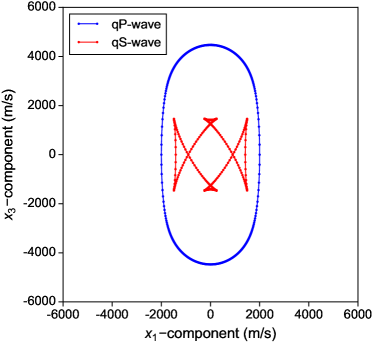
Figure 1: Wavefront curves in the 2D HTI medium with elasticity matrix (196).

In Meza-Fajardo and Papageorgiou (2008), the suggested values of damping ratios are $\xi_{1}=0.30$ and $\xi_{3}=0.25$ for this HTI medium. Their suggested value for damping ratio $\xi_{1}$ is much larger than the optimal damping ratio given in eq. (197), while their suggested value for $\xi_{3}$ is similar to the optimal damping ratio.

Figure 2 plots the values of eigenvalue derivatives of $\tilde{\mathbf{A}}$ under the optimal damping ratios in the $x_{1}$- and $x_{3}$-directions. In both panels, the blue curves represent the qP-wave eigenvalue derivatives, and the red curves are for the qS-wave eigenvalue derivatives. Clearly, the qS-wave gives rise to the large damping ratios along both axes. Note that we set the threshold $\epsilon=-0.005$, therefore, in both panels of Fig. 2, the maximum values of the eigenvalue derivatives are $-0.005$.

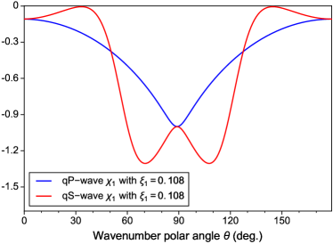
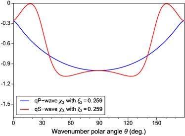
Figure 2: Eigenvalue derivatives of $\tilde{\mathbf{A}}$ of MPML in the (a) $x_{1}$- and (b) $x_{3}$-directions under calculated optimal damping ratios in eq. (197) for the 2D HTI medium with elasticity matrix (196).

We validate the effectiveness of our new MPML in numerical modeling of anisotropic elastic-wave progation. We use the rotated-staggered grid (RSG) finite-difference method Saenger et al. (2000) to solve the stress-velocity form elastic-wave equations (1)–(2). The RSG finite-difference method has 16th-order accuracy in space with optimal finite-difference coefficients Liu (2014). We compute the wavefield energy decay curves of our wavefield modelings to validate the effectiveness of MPML.

In our numerical modeling, the model is defined in a $400\times 400$ grid, and a PML of 30-node thickness are padded around the model domain. The grid size is 10 m in both the $x_{1}$- and $x_{3}$-directions. A vertical force vector source is located at the center of the computational domain, and a Ricker wavelet with a 10 Hz central frequency is used as the source time function. We simulate wave propagation for 20 s with a time interval of 1 ms, which is smaller than what is required to satisfy the stability condition (about 1.54 ms). Figure 3 shows the resulting wavefield energy curve under the optimal damping ratios in eq. (197) , together with three others under different eigenvalue derivative threshold $\epsilon$ values, or equivalently, different damping ratios. Figure 3 shows that within the 20 s of wave propagation, the MPML with our calculated damping ratios $\xi_{1}=0.108$ and $\xi_{3}=0.259$ is stable. These damping ratios are obtained under threshold value $\epsilon=-0.005$, meaning that the damping ratios have to ensure the eigenvalues derivatives $\chi_{1}$ and $\chi_{3}$ are not larger than $-0.005$ in the entire range of wavenumber direction.

We test the behavior of MPML under threshold $\epsilon=0.01$, or equivalently, $\xi_{1}=0.095$ and $\xi_{3}=0.248$, and show in Fig. 3 that the numerical modeling is stable. We further increase the threshold $\epsilon$ to be 0.05, and the MPML becomes unstable quickly after about 2 s. Finally, the conventional PML, which is equivalent to MPML under $\xi_{1}=\xi_{3}=0$, becomes unstable even earlier (before 1 s). These tests indicate that a small positive threshold $\epsilon$ may still result in a stable MPML. However, there is no simple method to determine how large this positive $\epsilon$ to ensure the numerical stability. In this HTI medium case, $\epsilon=0.01$ results in stability while $\epsilon=0.05$ results in instability. Because a negative threshold resulting in stable MPML is consistent with the stability theory presented by Meza-Fajardo and Papageorgiou (2008), we therefore should choose a negative threshold for the calculation of the optimal damping ratios to ensure that the resulting MPML is stable. This is also verified in the hereinafter numerical examples.

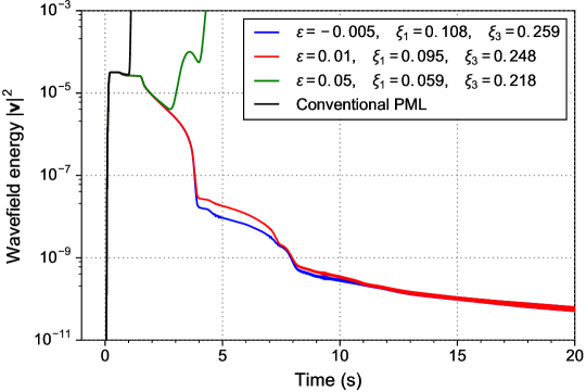
Figure 3: Wavefield energy decay curves under different eigenvalue derivative thresholds for the 2D HTI medium with elasticity matrix (196) within 20 s. Conventional PML can be considered as a special case of MPML with $\epsilon\gg 0$ or equivalently $\xi_{1}=\xi_{3}=0$.

Next, we rotate the aforementioned HTI medium with respect to the $x_{2}$-axis clockwise by $\pi/6$ to obtain a TTI medium represented by the following elasticity matrix:

$$\mathbf{C}=\left[\begin{array}[]{ccc}7.8125&7.6875&3.35585\\ &15.8125&3.57235\\ &&2.1875\end{array}\right],$$ (198)

with unit GPa. The rotation can be accomplished by rotation matrix (e.g., Slawinski, 2010). The wavefront curves in this TTI medium is shown in Fig. 4. Although this TTI medium is the rotation result of the HTI medium in the previous numerical example, it is not obvious how to change the damping ratios accordingly. We obtain the following optimal damping ratios of MPML under $\epsilon=-0.005$ using Algorithm 1:

$$\xi_{1}=0.157,\qquad\xi_{3}=0.226.$$ (199)

The eigenvalue derivatives under this set of damping ratios are shown in Fig. 5. The eigenvalue derivative curves are no longer symmetric with respect to $\theta=\pi/2$ (or has a period of $\pi/2$) as those for the 2D HTI medium (Fig. 2). Instead, they are periodic every $\pi$ angle, corresponding to the fact that there is always at least one symmetric axis for whatever kind of 2D anisotropic medium in the axis plane. These curves also indicate that, for 2D general anisotropic medium (TTI medium in this example), it is necessary to determine the values of eigenvalue derivatives within the range of $(0,\pi]$ instead of $(0,\pi/2]$. Using only the range $(0,\pi/2]$ can lead to a totally incorrect optimal value of $\xi_{1}$, since the maximum value of $\chi_{1}$ in the range $(0,\pi/2]$ is smaller than that in the range $(\pi/2,\pi]$ for this TTI medium. In other words, even though $\chi_{1}$ in $(0,\pi/2]$ indicates a stable MPML, the MPML may still be unstable since $\chi_{1}$ may be larger than zero in $(\pi/2,\pi]$. Therefore, for anisotropic media with symmetric axis not aligned with a coordinate axis, it is necessary to consider the values of $\chi_{i}$ in wavenumber direction $\theta\in(0,\pi]$. This statement is also true for 3D anisotropic media as shown in the hereinafter 3D numerical examples.

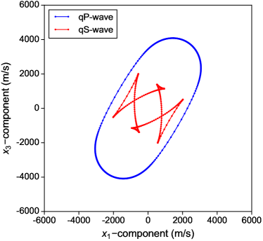
Figure 4: Wavefront curves in the 2D HTI medium with elasticity matrix (198).

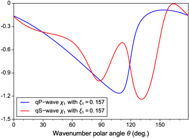
Figure 5: Eigenvalue derivatives of $\tilde{\mathbf{A}}$ of MPML in the (a) $x_{1}$- and (b) $x_{3}$-directions under calculated optimal damping ratios in eq. (199) for the 2D TTI medium with elasticity matrix (198).

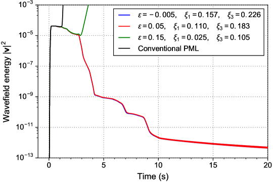
Figure 6: Wavefield energy decay curves under different eigenvalue derivative thresholds in the 2D TTI medium with elasticity matrix (198) within 20 s.

Figure 6 displays the wavefield energy decay curves for this TTI medium under the optimal damping ratios, as well as under damping ratios calculated with positive eigenvalue derivative thresholds. In this example, the wavefield energy decays gradually within 20 s for both cases with $\epsilon=-0.005$ and $\epsilon=0.05$. The numerical modeling with $\epsilon=0.15$ becomes unstable. For comparison, in the previous HTI case, $\epsilon=0.05$ results in an unstable MPML. These results further demonstrate that a positive eigenvalue derivative threshold should not be chosen to calculate the damping ratios, although a small positive $\epsilon$ might result in stable MPML. In contrast, a negative $\epsilon$ can always ensure the stability of MPML.

Our next numerical example uses a VTI medium defined by

$$\mathbf{C}=\left[\begin{array}[]{ccc}10.4508&4.2623&0\\ &7.5410&0\\ &&11.3934\end{array}\right].$$ (200)

The wavefront curves for this VTI medium are depicted in Fig. 7. The special feature of this VTI medium is that, in both the $x_{1}$- and $x_{3}$-directions, there exists serious qS-wave triplication phenomena. We obtain the following optimal damping ratios using Algorithm 1:

$$\xi_{1}=0.215,\qquad\xi_{3}=0.225.$$ (201)

The corresponding eigenvalue derivatives in the $x_{1}$- and $x_{3}$-directions are displayed in Fig. 8. Again, it is the qS-wave that causes the damping ratios to be large to stabilize PML. Figure 9 depicts the wavefield energy decay curves under different eigenvalue derivative thresholds. Similar with that of 2D TTI medium example, a positive threshold 0.05 can still stabilize PML, yet a value of 0.15 makes the MPML unstable. We choose a negative value of $\epsilon$ to ensure a stable MPML.

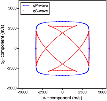
Figure 7: Wavefront curves in the 2D VTI medium with elasticity matrix (200).

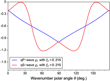
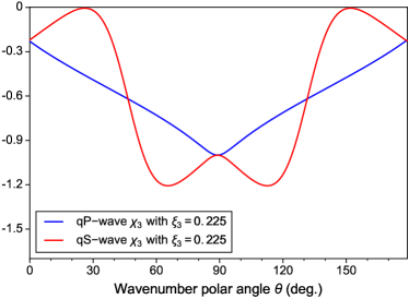
Figure 8: Eigenvalue derivatives of $\tilde{\mathbf{A}}$ of MPML in the (a) $x_{1}$- and (b) $x_{3}$-directions under calculated optimal damping ratios in eq. (201) for the 2D VTI medium with elasticity matrix (200).

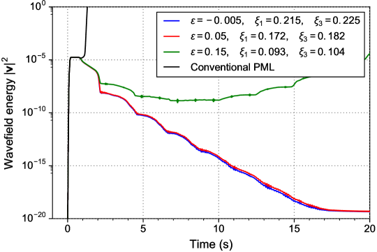
Figure 9: Wavefield energy decay curves under different eigenvalue derivative thresholds in the 2D VTI medium with elasticity matrix (200) within 20 s.

3.2 MPML for 3D anisotropic media

For 3D anisotropic media, we need to determine the optimal MPML damping ratios along all three coordinate directions. We use three different anisotropic media (a quasi-VTI medium, a quasi-TTI medium and a triclinic medium) to demonstrate the determination of optimal MPML damping ratios.

We first use a 3D anisotropic medium represented by the elasticity matrix

$$\mathbf{C}=\left[\begin{array}[]{cccccc}16.5&5&5&0&0&0\\ &16.5&5&0&0&0\\ &&6.2&0&0&0\\ &&&4.96&0&0\\ &&&&3.96&0\\ &&&&&5.96\end{array}\right].$$ (202)

This elasticity matrix is modified from the elasticity matrix of zinc (a VTI medium, or hexagonal anisotropic medium) to increase the complexity of the resulting wavefronts and the characteristics of the eigenvalue derivatives along all three directions. This modified elastic matrix still represents a physically feasible medium since it is easy to verify that it satisfies the following stability condition for anisotropic media Slawinski (2010):

$$\det\left[\begin{array}[]{ccc}C_{11}&\cdots&C_{1n}\\ \vdots&\ddots&\vdots\\ C_{1n}&\cdots&C_{nn}\end{array}\right]>0,$$ (203)

where $n=1,2,\cdots,6$. We call this anisotropic medium the quasi-VTI medium. Figure 10 shows the wavefront curves of this quasi-VTI medium on three axis planes.

For comparison, a standard 3D VTI medium can be expressed by its five independent elasticity constants as (e.g., Slawinski, 2010)

$$\mathbf{C}=\left[\begin{array}[]{cccccc}C_{11}&C_{12}&C_{13}&0&0&0\\ &C_{11}&C_{13}&0&0&0\\ &&C_{33}&0&0&0\\ &&&C_{44}&0&0\\ &&&&C_{44}&0\\ &&&&&\frac{C_{11}-C_{12}}{2}\end{array}\right].$$ (204)

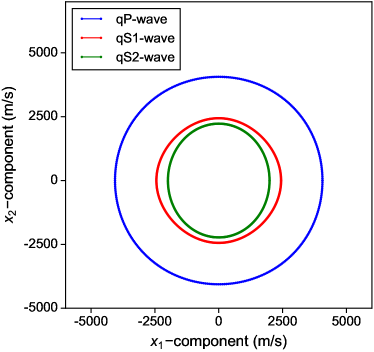
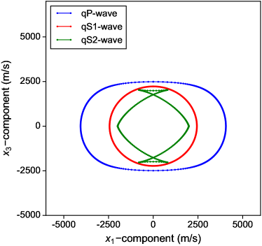
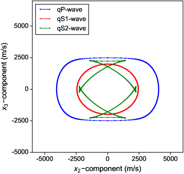
Figure 10: Wavefront curves in the 3D quasi-VTI medium with elasticity matrix (202) on the (a) $x_{1}x_{2}$ (b) $x_{1}x_{3}$ and (c) $x_{2}x_{3}$ axis plane. qS1 and qS2 represents the two qS-waves.

We calculate the optimal damping ratios for MPML using Algorithm 2, and obtain

$$\xi_{1}=0.088,\qquad\xi_{2}=0.131,\qquad\xi_{3}=0.041.$$ (205)

We plot the eigenvalue derivatives in the polar angle range $(0,\pi]$ and azimuth angle range $(0,\pi]$ for three axis directions in Fig. 11. Since the three symmetric axes of this VTI medium are aligned with three coordinate axes, the three eigenvalue derivatives are symmetric with respect to both $\theta=\pi/2$ and $\phi=\pi/2$ lines.

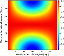
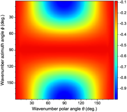
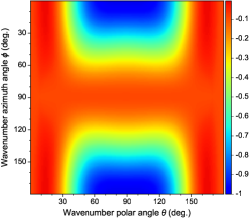
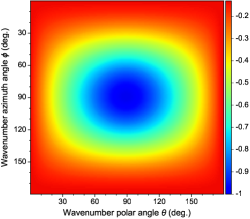
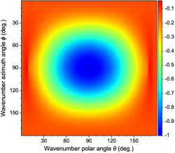
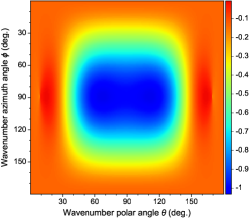
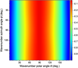
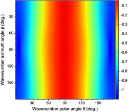
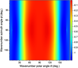
Figure 11: Eigenvalue derivatives of $\tilde{\mathbf{A}}$ of MPML in the (a)-(c) $x_{1}$-, (d)-(f) $x_{2}$-, and (g)-(i) $x_{3}$-directions under calculated optimal damping ratios in eq. (205) for the 3D quasi-VTI medium with elasticity matrix (202). (a), (d) and (g) represent qP-wave, (b), (e) and (h) represent qS1-wave, (c), (f) and (i) represent qS2-wave.

We conduct numerical wavefield modeling to verify the stability of MPML under these optimal damping ratios. The model is defined on a $400\times 400\times 400$ grid with a grid size of 10 m in all three directions. The thickness of PML layer is 25 grids. A vertical force vector is located at the center of the computational domain, and the source time function is a Ricker wavelet with a central frequency of 10 Hz. The time step size is 1 ms, which is smaller than the stability-required time step of 1.69 ms. A total of 15,000 time steps, i.e., 15 s, are simulated, and the wavefield energy curve is shown in Fig. 12. The blue curve in Fig. 12 is for the case with the optimal damping ratios in eq. (205). We also carry out a wavefield modeling with the eigenvalue derivative threshold $\epsilon=0.015$ and $\epsilon=0.025$. The MPMLs under these thresholds are unstable according to the corresponding wavefield energy variation curves in Fig. 12. As in the 2D MPML case, we should always choose a negative $\epsilon$ to stabilize MPML for 3D anisotropic media.

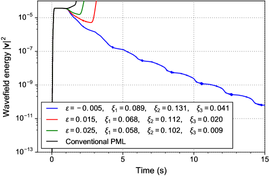
Figure 12: Wavefield energy decay curve in the 3D VTI medium with elasticity matrix (202).

Our next numerical example uses a rotation version of the aforementioned quasi-VTI medium. We rotate the quasi-VTI medium (202) with respect to the $x_{1}$-axis by 30 degrees, the $x_{2}$-axis by 50 degrees, and the $x_{3}$-axis by 25 degrees, and the resulting elasticity matrix for this quasi-TTI medium is given by

$$\mathbf{C}=\left[\begin{array}[]{cccccc}15.7930&4.1757&4.9651&0.1582&0.6529&-1.0343\\ &12.5979&4.1844&2.0903&0.8186&-1.7513\\ &&14.1587&1.9573&0.7643&-0.1606\\ &&&3.7879&-0.8909&0.8065\\ &&&&5.0750&0.7668\\ &&&&&4.3423\end{array}\right].$$ (206)

The corresponding wavefront curves are shown in Fig. 13.

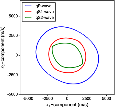
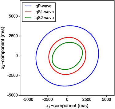
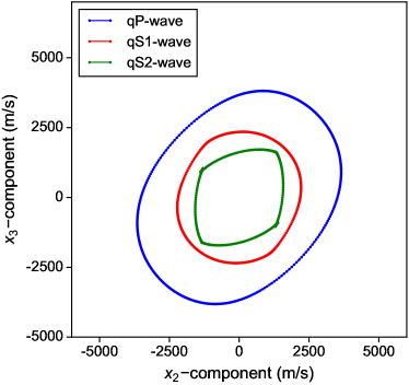
Figure 13: Wavefront curves in the 3D quasi-TTI medium with elasticity matrix (206) on the (a) $x_{1}x_{2}$ (b) $x_{1}x_{3}$ and (c) $x_{2}x_{3}$ axis plane. qS1 and qS2 represents the two qS-waves. qS-wave wavefronts seem to be less complicated compared with those of the 3D quasi-VTI medium (202) only because the qS-wave triplications are now out of axis planes after rotation.

Similar to the 3D quasi-VTI case, we obtain the following optimal damping ratios using Algorithm 2:

$$\xi_{1}=0.089,\qquad\xi_{2}=0.051,\qquad\xi_{3}=0.080.$$ (207)

The eigenvalue derivatives under this set of damping ratios for three axis directions are shown in Fig. 14. Obviously, for the quasi-TTI medium where the symmetric axes are not aligned with coordinate axes, the eigenvalue derivatives of all three wave modes along any coordinate axis is no longer symmetric about any $\theta$ or $\phi$ lines. Therefore, it is necessary to use the entire range of wavenumber polar angle $\theta$ and azimuth angle $\phi$, i.e., $(0,\pi]\times(0,\pi]$, to determine the optimal damping ratios.

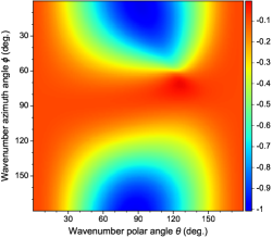
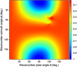
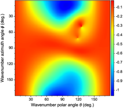
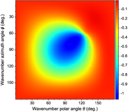
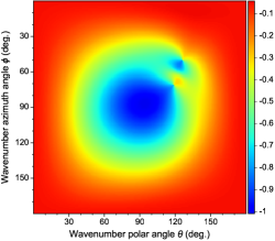
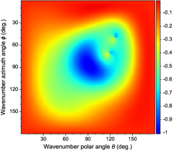
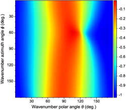
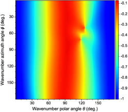
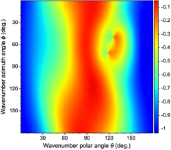
Figure 14: Eigenvalue derivatives of $\tilde{\mathbf{A}}$ of MPML in the (a)-(c) $x_{1}$-, (d)-(f) $x_{2}$-, and (g)-(i) $x_{3}$-directions under calculated optimal damping ratios in eq. (207) for the 3D quasi-TTI medium with elasticity matrix (206). (a), (d) and (g) represent qP-wave, (b), (e) and (h) represent qS1-wave, (c), (f) and (i) represent qS2-wave.

Figure 15 depicts the wavefield energy decays under the optimal damping ratios in eq. (207) and damping ratios with thresholds $\epsilon=0.05$ and $\epsilon=0.075$. For the case where $\epsilon=0.05$, the wavefield energy does not diverge immediately after maximum energy value occurred. Instead, the curve indicates a very slow energy decay after about 1 s. In contrast, the optimal MPML with threshold $\epsilon=-0.005$ shows a “normal” energy decay. Therefore, although the MPML with $\epsilon=0.05$ does not show energy divergence within 15 s, it fails to effectively absorb the outgoing wavefield, and we consider this as a “quasi-divergence.” Meanwhile, the MPML with $\epsilon=0.075$ shows an energy divergence after about 4 s. These results further demonstrate that the behavior of MPML with a positive eigenvalue derivative threshold is different and unpredictable for different kinds of anisotropic media. Figure 15 also shows that the conventional PML gives an unstable result.

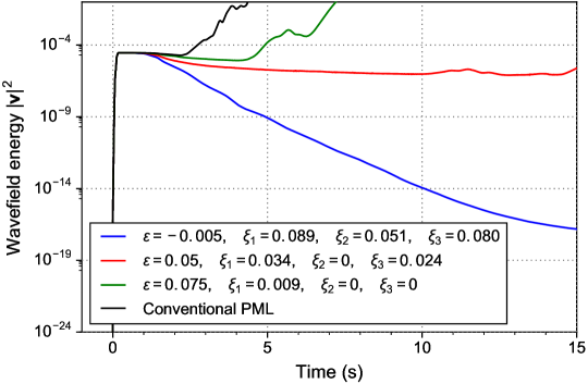
Figure 15: Wavefield energy decay curve in the 3D quasi-TTI medium with elasticity matrix (206).

Our last 3D numerical example is based on a triclinic anisotropic medium represented by

$$\mathbf{C}=\left[\begin{array}[]{cccccc}10&3.5&2.5&-5&0.1&0.3\\ &8&1.5&0.2&-0.1&-0.15\\ &&6&1&0.4&0.24\\ &&&5&0.35&0.525\\ &&&&4&-1\\ &&&&&3\end{array}\right],$$ (208)

with unit GPa. The wavefront curves on three axis planes are shown in Fig. 16.

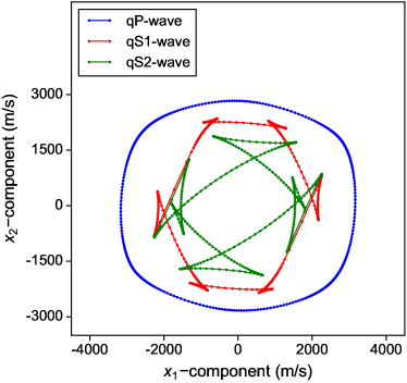
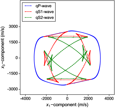
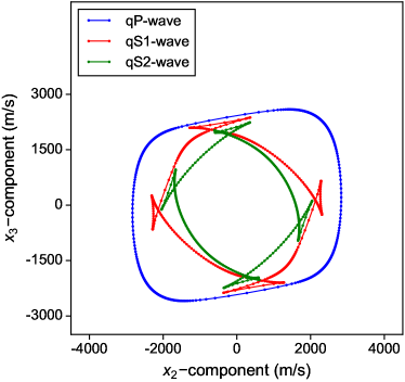
Figure 16: Wavefront curves in the 3D triclinic anisotropic medium with elasticity matrix (206) on the (a) $x_{1}x_{2}$ (b) $x_{1}x_{3}$ and (c) $x_{2}x_{3}$ axis plane. qS1 and qS2 represents the two qS-waves.

We solve for the optimal damping ratios for this triclinic anisotropic medium using Algorithm 2, and obtain the following optimal damping ratios with $\epsilon=-0.005$:

$$\xi_{1}=0.487,\qquad\xi_{2}=0.345,\qquad\xi_{3}=0.374.$$ (209)

The damping ratios for this anisotropic medium are unexpectedly very large compared with those for the heretofore 2D and 3D examples. We seek the reasons of these large damping ratios from the eigenvalue derivatives shown in Fig. 17, and find that it is the qS2-wave that leads to such large damping ratios to achieve a stable MPML. In fact, for the damping ratios in eq. (209), the corresponding eigenvalue derivatives of qP- and qS1-waves are far smaller than zero, yet the eigenvalue derivative of qS2-wave merely smaller than zero ($-0.005$ under our threshold setting), leading to a set of relatively large damping ratios for this 3D anisotropic medium.

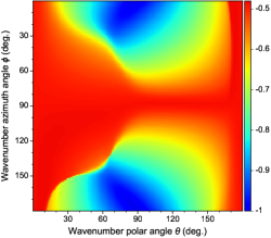
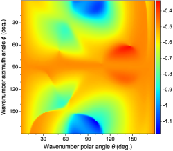
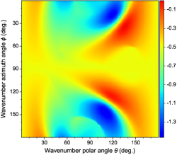
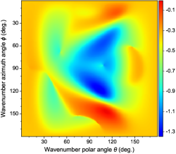
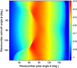
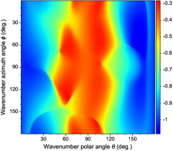
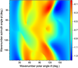
Figure 17: Eigenvalue derivatives of $\tilde{\mathbf{A}}$ of MPML in the (a)-(c) $x_{1}$-, (d)-(f) $x_{2}$-, and (g)-(i) $x_{3}$-directions under calculated optimal damping ratios in eq. (209) for the 3D triclinic anisotropic medium with elasticity matrix (208). (a), (d) and (g) represent qP-wave, (b), (e) and (h) represent qS1-wave, (c), (f) and (i) represent qS2-wave.

Our calculated optimal damping ratios result in a stable MPML, as indicated by the corresponding energy decay curve shown in Fig. 18. The wavefield energy decay curve with a threshold of $\epsilon=0.1$ displayed in Fig. 18 is surprisingly almost identical with that of $\epsilon=-0.005$. When using a threshold $\epsilon=0.4$, MPML become unstable, indicating that the positive threshold 0.4 is too large to make MPML stable. This verifies again that, although a positive threshold might result in stable MPML, we should use a negative threshold to ensure a stable MPML for general anisotropic media. This is consistent with the stability condition described in Meza-Fajardo and Papageorgiou (2008), and is perhaps the only practical method to stabilize PML using nonzero damping ratios.

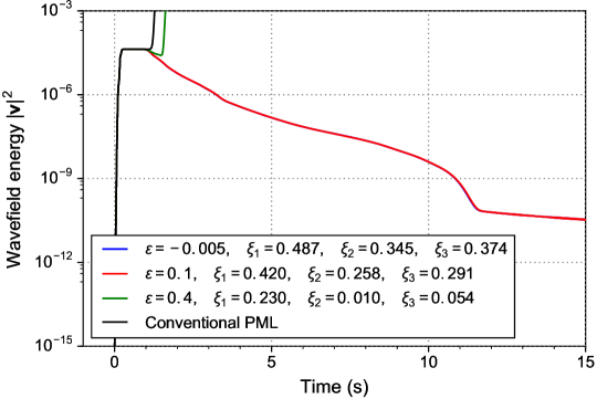
Figure 18: Wavefield energy decay curve in the 3D triclinic anisotropic medium with elasticity matrix (208). The blue curve ($\epsilon=-0.005$) and red curve ($\epsilon=0.1$) are almost identical.

4 Conclusions

A definite analytic method for determining the optimal damping ratios of multi-axis perfectly matched layers (MPML) is generally impossible for 3D general anisotropic media with possible all nonzero elasticity parameters. We have developed a new method to efficiently determine the optimal damping ratios of MPML for absorbing unwanted, outgoing propagating waves in 2D and 3D general anisotropic media. This numerical approach is very straightforward using the left and right eigenvectors of the damped system coefficient matrix. We have used six numerical modeling examples of elastic-wave propagation in 2D and 3D anisotropic media to demonstrate that our new algorithm can effectively and correctly provide the optimal MPML damping ratios for even very complex, general anisotropic media.

5 Acknowledgments

This work was supported by U.S. Department of Energy through contract DE-AC52-06NA25396 to Los Alamos National Laboratory (LANL). The computation was performed using super-computers of LANL’s Institutional Computing Program.

References

-
Bécache et al. (2003)
Bécache, E., Fauqueux, S., Joly, P., 2003. Stability of perfectly matched
layers, group velocities and anisotropic waves. Journal of Computational
Physics 188 (2), 399 – 433.
URL http://www.sciencedirect.com/science/article/pii/S0021999103001840 -
Berenger (1994)
Berenger, J.-P., 1994. A perfectly matched layer for the absorption of
electromagnetic waves. Journal of Computational Physics 114 (2), 185 – 200.
URL http://www.sciencedirect.com/science/article/pii/S0021999184711594 - Carcione (2007) Carcione, J. M., 2007. Wave fields in real media: Wave propagation in anisotropic, anelastic, porous and electromagnetic media (Second Edition). Elsevier, Amsterdam, Netherlands.
-
Cerjan et al. (1985)
Cerjan, C., Kosloff, D., Kosloff, R., Reshef, M., 1985. A nonreflecting
boundary condition for discrete acoustic and elastic wave equations.
Geophysics 50 (4), 705–708.
URL http://geophysics.geoscienceworld.org/content/50/4/705 -
Clayton and Engquist (1977)
Clayton, R., Engquist, B., 1977. Absorbing boundary conditions for acoustic and
elastic wave equations. Bulletin of the Seismological Society of America
67 (6), 1529–1540.
URL http://bssa.geoscienceworld.org/content/67/6/1529 -
Collino and Tsogka (2001)
Collino, F., Tsogka, C., 2001. Application of the perfectly matched absorbing
layer model to the linear elastodynamic problem in anisotropic heterogeneous
media. Geophysics 66 (1), 294–307.
URL http://dx.doi.org/10.1190/1.1444908 -
de la Puente et al. (2007)
de la Puente, J., Käser, M., Dumbser, M., Igel, H., 2007. An arbitrary
high-order discontinuous Galerkin method for elastic waves on unstructured
meshes – IV. Anisotropy. Geophysical Journal International 169 (3),
1210–1228.
URL http://dx.doi.org/10.1111/j.1365-246X.2007.03381.x -
Dmitriev and Lisitsa (2011)
Dmitriev, M. N., Lisitsa, V. V., 2011. Application of M-PML reflectionless
boundary conditions to the numerical simulation of wave propagation in
anisotropic media. Part I: Reflectivity. Numerical Analysis and Applications
4 (4), 271–280.
URL http://dx.doi.org/10.1134/S199542391104001X -
Drossaert and Giannopoulos (2007)
Drossaert, F. H., Giannopoulos, A., 2007. A nonsplit complex frequency-shifted
pml based on recursive integration for fdtd modeling of elastic waves.
Geophysics 72 (2), T9–T17.
URL http://dx.doi.org/10.1190/1.2424888 - Hastings et al. (1996) Hastings, F. D., Schneider, J. B., Broschat, S. L., 1996. Application of the perfectly matched layer (PML) absorbing boundary condition to elastic wave propagation. The Journal of the Acoustical Society of America 100 (5).
-
Higdon (1986)
Higdon, R. L., Oct. 1986. Absorbing boundary conditions for difference
approximations to the multi-dimensional wave equation. Math. Comput.
47 (176), 437–459.
URL http://dx.doi.org/10.2307/2008166 -
Higdon (1987)
Higdon, R. L., 1987. Numerical absorbing boundary conditions for the wave
equation. Mathematics of Computation 49 (179), 65–90.
URL http://www.jstor.org/stable/2008250 -
Komatitsch et al. (2000)
Komatitsch, D., Barnes, C., Tromp, J., 2000. Simulation of anisotropic wave
propagation based upon a spectral element method. Geophysics 65 (4),
1251–1260.
URL http://dx.doi.org/10.1190/1.1444816 -
Komatitsch and Martin (2007)
Komatitsch, D., Martin, R., 2007. An unsplit convolutional perfectly matched
layer improved at grazing incidence for the seismic wave equation. Geophysics
72 (5), SM155–SM167.
URL http://dx.doi.org/10.1190/1.2757586 -
Komatitsch and Tromp (2003)
Komatitsch, D., Tromp, J., 2003. A perfectly matched layer absorbing boundary
condition for the second-order seismic wave equation. Geophysical Journal
International 154 (1), 146–153.
URL http://dx.doi.org/10.1046/j.1365-246X.2003.01950.x -
Liao et al. (1984)
Liao, Z.-F., Huang, K.-L., Yang, B.-P., Yuan, Y.-F., 1984. A transmitting
boundary for transient wave analyses. Science China: Mathematics 27 (10),
1063.
URL http://math.scichina.com:8081/sciAe/EN/abstract/article_379434.shtml -
Liu (2014)
Liu, Y., 2014. Optimal staggered-grid finite-difference schemes based on
least-squares for wave equation modelling. Geophysical Journal International
197, 1033–1047.
URL http://gji.oxfordjournals.org/content/early/2014/02/20/gji.ggu032.abstract -
Long and Liow (1990)
Long, L. T., Liow, J. S., 1990. A transparent boundary for finite-difference
wave simulation. Geophysics 55 (2), 201–208.
URL http://geophysics.geoscienceworld.org/content/55/2/201 -
Martin and Komatitsch (2009)
Martin, R., Komatitsch, D., 2009. An unsplit convolutional perfectly matched
layer technique improved at grazing incidence for the viscoelastic wave
equation. Geophysical Journal International 179 (1), 333–344.
URL http://dx.doi.org/10.1111/j.1365-246X.2009.04278.x - Martin et al. (2010) Martin, R., Komatitsch, D., Gedney, S. D., Bruthiaux, E., 2010. A high-order time and space formulation of the unsplit perfectly matched layer for the seismic wave equation using auxiliary differential equations (ADE-PML). Computer Modeling in Engineering & Sciences 56 (1), 17–40.
-