New concept for pairing anti-halo effect as a localized wave packet of quasi-particle

Abstract

The pairing anti-halo effect is a phenomenon that a pairing correlation suppresses a divergence of nuclear radius, which happens for single-particle states with orbital angular momenta of $l$ = 0 and 1 in the limit of vanishing binding energy. While this effect has mainly been discussed in terms of Hartree-Fock-Bogoliubov (HFB) theory, we here use a three-body model and provide its new intuitive concept as a localized wave packet for a quasi-particle, that is, a coherent superposition of a weakly bound and continuum wave functions due to a pairing interaction. We show that the one-particle density in the three-body model can be directly expressed with such quasi-particle wave functions, which have a close analog to wave functions in the HFB approximation.

I Introduction

It has been known well that, in the limit of vanishing binding energy, the root-mean-square radius diverges for a wave function in a short range potential well with orbital angular momenta of $l$ = 0 and 1 RJM92 ; Jensen04 . Halo nuclei, which are characterized by an extended density distribution Tanihata85 ; Tanihata88 , have been interpreted to be due to such divergence with a single-particle wave function for $l$ = 0 and 1 S92 . See Refs. HTS13 ; TSK13 ; SH15 for recent review articles on halo nuclei.

For even-even nuclei, the pairing correlation among valence neutrons plays a decisive role in the structure of weakly bound nuclei Doba96 ; BE91 ; EBH97 ; HS05 . Bennaceur, Dobaczewski, and Ploszajczak have demonstrated that the root-mean-square radius does not diverge for even-even nuclei as the pairing correlation largely suppresses the halo structure in odd-mass nuclei, which has been referred to as the pairing anti-halo effect BDP00 . In Refs. HS11 ; HS12 ; HS12-2 , we have argued that the odd-even staggerings observed in reaction cross sections Takechi12 ; Takechi14 can be interpreted in terms of the pairing anti-halo effect (see also Refs. Sasabe13 ; MY14 ).

The pairing anti-halo effect has been studied using mainly the Hartree-Fock-Bogoliubov (HFB) method BDP00 ; CRM14 ; GYSG06 ; Y05 . In this approach, the pairing anti-halo effect occurs because the quasi-particle energy remains a finite value even when a single-particle energy vanishesBDP00 . A key issue for this argument is that the pairing gap needs to be finite in the zero binding limit. Many HFB calculations have actually shown that it is indeed the case BDP00 ; HS11 ; HS12 ; HS12-2 ; CRM14 ; GYSG06 ; Y05 , leading to a suppression of the halo structure in even-even systems.

Although the HFB method provides a clear mathematical interpretation of the pairing anti-halo effect, its physical mechanism is less transparent. The aim of this paper is to propose a more intuitive idea on the pairing anti-halo effect, using a three-body model with a core nucleus and two valence neutrons. This model is formulated with a simpler single-particle basis, providing a complementary interpretation to the one based on the HFB method.

The paper is organized as follows. In Sec. II, we first show how the pairing anti-halo effect is realized in the HFB method. We then introduce the three-body model and discuss the pairing anti-halo effect in this model. In Sec. III, we introduce a quasi-particle wave function within the three-body model and investigate its structure. We show that a coherent superposition of a weakly bound state and continuum states is a key ingredient of the pairing anti-halo effect. We then summarize the paper in Sec. IV.

II Pairing anti-halo effect

II.1 Hartree-Fock-Bogoliubov method

Before we discuss the pairing anti-halo effect with a three-body model, we first show how it is understood in the HFB method. This is also to clarify the notation used in this paper.

For a two-body system which consists of a valence neutron and a core nucleus, we assume that the wave function for the relative motion obeys the Schrödinger equation given by,

$$\hat{h}\,\psi_{nljm}(\mbox{\boldmath$r$})=\left[-\frac{\hbar^{2}}{2\mu}\mbox{\boldmath$\nabla$}^{2}+V(r)\right]\psi_{nljm}(\mbox{\boldmath$r$})=\epsilon_{nlj}\,\psi_{nljm}(\mbox{\boldmath$r$}),$$ (1)

where $\mu$ is the reduced mass and $V(r)$ is the potential between the valence neutron and the core nucleus. We have assumed that $V(r)$ is local and has spherical symmetry so that the wave function is characterized by the orbital angular momentum $l$, the total angular momentum $j$ and its $z$-component, $m$, as well as the radial quantum number, $n$. Here, $\epsilon_{nlj}$ is the energy eigenvalue.

For simplicity, we consider only an $s$ wave solution of this Schrödinger equation. The radial wave function $u_{nlj}(r)$, defined with the spin-angular function, ${\cal Y}_{jlm}(\hat{\mbox{\boldmath$r$}})$, by

$$\psi_{nljm}(\mbox{\boldmath$r$})=\frac{u_{nlj}(r)}{r}{\cal Y}_{jlm}(\hat{\mbox{\boldmath$r$}}),$$ (2)

behaves asymptotically as,

$$u_{nlj}(r)\sim\exp(-\alpha_{nlj}\,r),$$ (3)

where $\alpha_{nlj}$ is defined as $\alpha_{nlj}=\sqrt{2\mu|\epsilon_{nlj}|/\hbar^{2}}$. The expectation value of $r^{2}$ then reads,

$$\langle r^{2}\rangle\sim\frac{1}{2\alpha_{nlj}^{2}}=\frac{\hbar^{2}}{4\mu|\epsilon_{nlj}|},$$ (4)

which apparently diverges in the limit of $\epsilon_{nlj}\to 0$.

In many-body systems with the pairing correlation, one may consider the HFB equations given by Doba96 ; Doba84 ,

$$\left(\begin{array}[]{cc}\hat{h}-\lambda&\Delta(r)\\ \Delta(r)&-\hat{h}+\lambda\end{array}\right)\left(\begin{array}[]{c}U_{nljm}(\mbox{\boldmath$r$})\\ V_{nljm}(\mbox{\boldmath$r$})\end{array}\right)=E_{nlj}\left(\begin{array}[]{c}U_{nljm}(\mbox{\boldmath$r$})\\ V_{nljm}(\mbox{\boldmath$r$})\end{array}\right),$$ (5)

where $\hat{h}$ is the mean-field Hamiltonian given in Eq. (1), $\Delta(r)$ is the pairing potential, and $\lambda$ is the chemical potential. We have again assumed that both the mean-field potential in $\hat{h}$ and the pairing potential, $\Delta(r)$, are spherical and local functions of $r$. In the HFB equations, Eq. (5), $E_{nlj}$ is a quasi-particle energy and $U_{nljm}(\mbox{\boldmath$r$})$ and $V_{nljm}(\mbox{\boldmath$r$})$ are the upper and the lower components of a quasi-particle wave function, respectively. These are ortho-normalized according to,

$$\int d\mbox{\boldmath$r$}[U^{*}_{\alpha}(\mbox{\boldmath$r$})U_{\beta}(\mbox{\boldmath$r$})+V^{*}_{\alpha}(\mbox{\boldmath$r$})V_{\beta}(\mbox{\boldmath$r$})]=\delta_{\alpha,\beta},$$ (6)

where $\alpha$ and $\beta$ are shorthanded notations for $(njlm)$. The one-particle density, $\rho(r)$, is given in terms of $V_{nljm}(\mbox{\boldmath$r$})$ by,

$$\rho(r)=\sum_{n}\sum_{j,l,m}|V_{nljm}(\mbox{\boldmath$r$})|^{2}.$$ (7)

In the BCS approximation, $V_{nljm}(\mbox{\boldmath$r$})$ is expressed by a product of the occupation factor $v_{nlj}^{BCS}$ and the single-particle wave function, $\psi_{nljm}(\mbox{\boldmath$r$})$ Doba96 ; HS05-2 . In contrast, in the HFB, the asymptotic form of the radial part for the lower component, defined similarly to Eq. (3), reads Doba96 ,

$$v_{nlj}(r)\sim\exp(-\beta_{nlj}\,r),$$ (8)

for $l=0$, where $\beta_{nlj}$ is given as $\beta_{nlj}=\sqrt{2\mu(E_{nlj}-\lambda)/\hbar^{2}}$. The expectation value of $r^{2}$ with this wave function reads,

$$\langle r^{2}\rangle\sim\frac{1}{2\beta_{nlj}^{2}}.$$ (9)

Notice that the quasi-particle energy, $E_{nlj}$, is given in the BCS approximation as, $E_{nlj}=\sqrt{(\epsilon_{nlj}-\lambda)^{2}+\Delta_{nlj}^{2}}$, where $\Delta_{nlj}$ is the pairing gap. This implies that $E_{nlj}$ behaves as $E_{nlj}\sim\Delta_{nlj}$ in the zero binding limit with $\lambda\sim\epsilon_{nlj}\sim 0$. The expectation value of $r^{2}$ then reads,

$$\langle r^{2}\rangle\sim\frac{\hbar^{2}}{4\mu\,\Delta_{nlj}},$$ (10)

which remains finite as long as the pairing gap, $\Delta_{nlj}$, is finite. This is nothing but the pairing anti-halo effect proposed in Ref. BDP00 . An essential point for the pairing anti-halo effect is that the single-particle energy, $\epsilon_{nlj}$, is replaced by the quasi-particle energy, $E_{nlj}-\lambda$, reflecting the pairing correlation, which then induces a shrinkage of wave function according to Eq. (8).

II.2 Three-body model

In order to achieve a simple but still physical concept for the pairing anti-halo effect, let us now introduce a three-body model which consists of the core nucleus and two valence neutrons. The Hamiltonian for the three-body model reads EBH97 ; HS05 ,

$$H=\hat{h}(1)+\hat{h}(2)+v_{\rm pair}(\mbox{\boldmath$r$}_{1},\mbox{\boldmath$r$}_{2})+\frac{\mbox{\boldmath$p$}_{1}\cdot\mbox{\boldmath$p$}_{2}}{m_{c}},$$ (11)

where the single-particle Hamiltonian, $\hat{h}$, is the same as the one in Eq. (1) and $v_{\rm pair}(\mbox{\boldmath$r$}_{1},\mbox{\boldmath$r$}_{2})$ is a pairing interaction between the two valence neutrons. The last term in this equation is the two-body part of the recoil kinetic energy of the core nucleus, whose mass is denoted by $m_{c}$.

Using the eigen-functions of the single-particle Hamiltonian $\hat{h}$, that is, the wave functions $\psi_{nljm}(\mbox{\boldmath$r$})$ in Eq. (1), the two-particle wave function for the ground state of the three-body system with spin-parity of $J^{\pi}=0^{+}$ is given as,

$$\Psi(\mbox{\boldmath$r$}_{1},\mbox{\boldmath$r$}_{2})=\sum_{n,n^{\prime},l,j}C_{nn^{\prime}lj}\Psi_{nn^{\prime}lj}^{(2)}(\mbox{\boldmath$r$}_{1},\mbox{\boldmath$r$}_{2}),$$ (12)

with

$$\Psi_{nn^{\prime}lj}^{(2)}(\mbox{\boldmath$r$}_{1},\mbox{\boldmath$r$}_{2}) = [\psi_{nlj}(\mbox{\boldmath$r$}_{1})\psi_{n^{\prime}lj}(\mbox{\boldmath$r$}_{2})]^{J=0},$$

$$= \sum_{m}\frac{(-1)^{j-m}}{\sqrt{2j+1}}\,\psi_{nljm}(\mbox{\boldmath$r$}_{1})\psi_{n^{\prime}lj-m}(\mbox{\boldmath$r$}_{2}).$$

(For simplicity of the notation, we do not use here the anti-symmetrized basis BE91 . The anti-symmetrization is realized by setting $C_{nn^{\prime}jl}=C_{n^{\prime}nlj}\equiv\tilde{C}_{nn^{\prime}lj}/\sqrt{2}$ in Eq. (12)). The one-particle density constructed with this two-particle wave function is then given by BE91 ,

$$\rho(\mbox{\boldmath$r$}) = \int d\mbox{\boldmath$r$}^{\prime}|\Psi(\mbox{\boldmath$r$},\mbox{\boldmath$r$}^{\prime})|^{2},$$

$$= \sum_{n,n^{\prime},\tilde{n}}\sum_{j,l,m}\frac{C^{*}_{nn^{\prime}lj}C_{\tilde{n}n^{\prime}lj}}{2j+1}\,\psi_{nljm}^{*}(\mbox{\boldmath$r$})\psi_{\tilde{n}ljm}(\mbox{\boldmath$r$}).$$

Using the spherical reduction for the wave functions (see Eq. (2)), one can show that the one-particle density is expressed as BE91 ,

$$\rho(r)=\frac{1}{4\pi}\,\sum_{n,n^{\prime},\tilde{n}}\sum_{j,l,m}C^{*}_{nn^{\prime}lj}C_{\tilde{n}n^{\prime}lj}\phi^{*}_{nlj}(r)\phi_{\tilde{n}lj}(r),$$ (17)

where $\phi_{nlj}$ is defined as $\phi_{nlj}(r)=u_{nlj}(r)/r$.

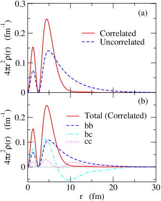
Figure 1: (Upper panel) The correlated (the solid line) and the uncorrelated (the dashed line) one-particle densities obtained with the three-body model for ²⁴O. Only the $s$-wave single-particle states are included in the calculations. In the uncorrelated case, the two valence neutrons occupy the 2$s_{1/2}$ state at $\epsilon=-0.275$ MeV, while they are scattered into the continuum states in the correlated case. A zero-range pairing interaction is employed, which yields the ground state energy of $E_{\rm g.s.}=-2.46$ MeV. (Lower panel) The decomposition of the correlated density into three components. The (bb) component (the dashed line) corresponds to the one in which both of the two valence neutrons occupy the bound 2$s_{1/2}$ state, while in the (bc) component shown by the dot-dashed line, one of them is scattered to a continuum state. The (cc) component shown by the dotted line corresponds to the one in which both of the valence neutrons are scattered into continuum states. The total correlated density is also shown by the solid line.

The upper panel of Fig. 1 shows a one-particle density in the three-body model. To draw this figure, we consider the ²⁴O nucleus (²⁴O = ²²O + $n$ + $n$), and employ a contact pairing interaction, $v_{\rm pair}(\mbox{\boldmath$r$},\mbox{\boldmath$r$}^{\prime})=-g\delta(\mbox{\boldmath$r$}-\mbox{\boldmath$r$}^{\prime})$, with $g=1374$ MeV fm³, together with the cutoff energy of $E_{\rm cut}=10$ MeV. The continuum states are discretized with the box boundary condition with the box size of $R_{\rm box}$ = 30 fm. We use a Woods-Saxon potential for the mean-field potential, $V(r)$, with the radius parameter of $R$ = 3.5 fm and the diffuseness parameter of $a$ = 0.67 fm HS05 . The depth of the Woods-Saxon potential is somewhat arbitrarily chosen to be $V_{0}$ = $-34.56$ MeV, which has the 2$s_{1/2}$ state at $-0.275$ MeV. For simplicity of the discussion, we include only $l$ = 0 in Eq. (12), for which the 1$s_{1/2}$ state is assumed to be occupied by the core nucleus and is explicitly excluded in the summation. In this model space, there are one bound state, 2$s_{1/2}$, at $\epsilon=-0.275$ MeV, and five discretized $s$-wave continuum states up to 10 MeV. This calculation yields the ground state energy of $E_{\rm g.s.}=-2.46$ MeV.

The dashed line in the figure shows the one-particle density in the absence of the pairing interaction, which is proportional to the square of the 2$s_{1/2}$ wave function, that is, $\rho(r)=|\phi_{2s_{1/2}}(r)|^{2}/4\pi$. Since the 2$s_{1/2}$ state is a weakly bound $s$-wave state, the resultant density has an extended long tail. In contrast, in the correlated density distribution shown by the solid line, the density distribution is considerably shrunk compared to the uncorrelated density. The root-mean-square radii are $\sqrt{\langle r^{2}\rangle}$ = 5.18 and 8.83 fm for the correlated and the uncorrelated cases, respectively. This is a clear manifestation of the pairing anti-halo effect discussed in the previous sub-section.

The lower panel of Fig. 1 shows a decomposition of the correlated density. Here, we decompose it into three components, that is, (i) (bb): both $n$ and $\tilde{n}$ in Eq. (17) belong to the weakly bound state, 2$s_{1/2}$, (ii) (bc): one of them belongs to the bound state while the other belongs to a continuum state, and (iii) (cc): both of them belong to continuum states. The (bb) component in fact has the same radial profile as the uncorrelated density shown in the upper panel, having an extended tail. The (bc) component behaves similarly to the (bb) component inside the potential, while it has the opposite sign to the (bb) component in the tail region. Because of this, the density in the inner part is enhanced while the (bb) and (bc) components are largely canceled out in the outer part. One can thus find that the scattering of a particle to the continuum spectrum due to the pairing interaction plays an essential role in the pairing anti-halo effect. The (cc) component, on the other hand, provides only a small portion of the correlated density, even though it is not negligible. This component is positive in a wide range of radial coordinate, as one can see in the figure.

III Quasi-particle wave function in the three-body model

In order to get a deeper insight into the pairing anti-halo effect in the three-body model, we next re-express the one-particle density in a different form. To this end, we first notice that the two-particle wave function, Eq. (12), is expressed as,

$$\Psi(\mbox{\boldmath$r$}_{1},\mbox{\boldmath$r$}_{2})=\sum_{n^{\prime}}\sum_{l,j}\,[\tilde{\psi}_{n^{\prime}lj}(\mbox{\boldmath$r$}_{1})\psi_{n^{\prime}lj}(\mbox{\boldmath$r$}_{2})]^{J=0},$$ (18)

with

$$\tilde{\psi}_{n^{\prime}ljm}(\mbox{\boldmath$r$})\equiv\sum_{n}C_{nn^{\prime}lj}\,\psi_{nljm}(\mbox{\boldmath$r$}).$$ (19)

The one-particle density, Eqs. (LABEL:rho1-0) and (17), is then given as,

$$\rho(\mbox{\boldmath$r$}) = \sum_{k}\sum_{j,l,m}\frac{1}{2j+1}\,|\tilde{\psi}_{kljm}(\mbox{\boldmath$r$})|^{2},$$ (20)

$$= \frac{1}{4\pi}\,\sum_{k}\sum_{j,l}\left|\frac{\tilde{u}_{klj}(r)}{r}\right|^{2},$$ (21)

where $\tilde{u}_{klj}(r)$ is defined as,

$$\tilde{u}_{klj}(r)\equiv\sum_{n}C_{nklj}\,u_{nlj}(r).$$ (22)

Notice that this is in a similar form to the one-particle wave function in the Hartree-Fock-Bogoliubov approximation, especially if one expands the quasi-particle wave function, $V_{kljm}$, on the Hartree-Fock basis, $\psi_{nljm}$ Gall94 ; Terasaki96 ; HS05-2 . For this reason, we shall call $\tilde{\psi}_{n^{\prime}ljm}(\mbox{\boldmath$r$})$ a “quasi-particle” wave function hereafter. Notice that the quasi-particle wave functions $\tilde{\psi}_{nljm}$ are not orthonormalized, just the same as the HFB wave functions $V_{nljm}$ (see Eq. (6)).

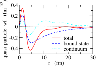
Figure 2: The radial part of the quasi-particle wave function, $\tilde{u}_{2s_{1/2}}(r)$, defined by Eq. (22), for the weakly bound 2$s_{1/2}$ state. The solid line shows the total wave function, while the dashed and the dot-dashed lines denote its bound state and continuum state contributions as defined by Eq. (III), respectively.

The solid line in Fig. 2 shows the radial dependence of the quasi-particle wave function for the weakly-bound 2$s_{1/2}$ state, that is, $\tilde{u}_{klj}(r)$ with $(klj)=2s_{1/2}$, for the three-body Hamiltonian introduced in the previous subsection. The dashed and the dot-dashed lines show its decomposition into the bound state and the continuum state contributions, respectively. They are defined as

$$\tilde{u}_{klj}(r) = \tilde{u}^{(b)}_{klj}(r)+\tilde{u}^{(c)}_{klj}(r),$$

$$= \sum_{n=2s_{1/2}}C_{nklj}\,u_{nlj}(r)+\sum_{n={\rm cont.}}C_{nklj}\,u_{nlj}(r).$$

One can see that the main feature of this quasi-particle wave function is similar to the one-particle density shown in Fig. 1 (b). That is, the bound state and the continuum state contributions are largely canceled with each other outside the potential while the two components contribute coherently in the inner region. We notice that the localization due to a coherent superposition of continuum states is the same mechanism as a formation of a localized wave packet. This is an essential ingredient of the pairing anti-halo effect, that is, a formation of localized wave packet induced by a pairing interaction.

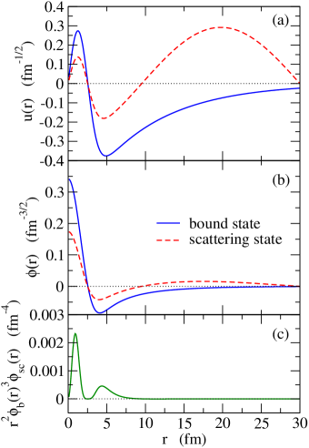
Figure 3: Figs. 3(a) and 3(b): The radial component of the wave functions for the weakly bound 2$s_{1/2}$ state (the solid line) and the lowest discretized $s$-wave state at $\epsilon$ = 0.51 MeV (the dashed line). Fig. 3(b) shows the radial wave function $\phi(r)$ while Fig. 3(a) shows $u(r)\equiv r\phi(r)$. Fig. 3(c): the integrand of the matrix element for the zero-range pairing interaction between the components $[\psi_{b}(\mbox{\boldmath$r$})\psi_{b}(\mbox{\boldmath$r$}^{\prime})]$ and ${\cal A}[\psi_{b}(\mbox{\boldmath$r$})\psi_{c}(\mbox{\boldmath$r$}^{\prime})]$, where ${\cal A}$ is the anti-symmetrizer and $\psi_{b}$ and $\psi_{c}$ are the wave functions for the weakly bound state and the lowest continuum state, respectively.

A question still remains concerning why the superposition is in such a way that the tail part of the bound wave function is suppressed. In order to clarify this point, let us strict ourselves only to two single-particle states, one is the weakly bound 2$s_{1/2}$ state at $\epsilon_{b}=-0.275$ MeV and the other is the lowest discretized $s$-wave continuum state. For the potential given in the previous section, the latter state is at $\epsilon_{c}$ = 0.51 MeV for $R_{\rm box}$ = 30 fm. Figs. 3(a) and 3(b) show the radial part of the wave functions for these states. The solid and the dashed lines correspond to the bound state and the scattering states, respectively. Fig. 3(b) shows the radial wave functions, $\phi(r)$, while Fig. 3(a) shows $u(r)=r\phi(r)$. In the inner part, the two wave functions behave similarly to each other, because the absolute value of the single-particle energies, $|\epsilon|$, is small for both the states, so that $V(r)-\epsilon\sim V(r)$. In the outer region where the potential $V(r)$ disappears, the two wave functions should behave differently. Since they behave similarly in the inner region, the two wave functions have to have opposite sign in the outer region in order to fulfill the orthogonal condition.

With these two single-particle states, we assume, for simplicity, that the two-particle wave function is given by,

$$\Psi(\mbox{\boldmath$r$}_{1},\mbox{\boldmath$r$}_{2})=C_{bb}\,\psi_{b}(\mbox{\boldmath$r$}_{1})\psi_{b}(\mbox{\boldmath$r$}_{2})+C_{bc}\,{\cal A}[\psi_{b}(\mbox{\boldmath$r$}_{1})\psi_{c}(\mbox{\boldmath$r$}_{2})],$$ (25)

where $\psi_{b}$ and $\psi_{c}$ are the bound and the scattering wave functions, respectively, and ${\cal A}$ is the anti-symmetrizer. The coefficients $C_{bb}$ and $C_{bc}$ are obtained by solving the eigen-value equation,

$$\left(\begin{array}[]{cc}\epsilon_{bb}&F\\ F&\epsilon_{bc}\end{array}\right)\left(\begin{array}[]{c}C_{bb}\\ C_{bc}\end{array}\right)=E\left(\begin{array}[]{c}C_{bb}\\ C_{bc}\end{array}\right),$$ (26)

where $\epsilon_{bb}$ and $\epsilon_{bc}$ are the diagonal components of the three-body Hamiltonian including the pairing matrix elements (in the present case, $\epsilon_{bb}$ and $\epsilon_{bc}$ are $-2.16$ and $-0.53$ MeV, respectively). $F$ is the matrix element of the pairing interaction between the two configurations, that is,

$$F=-\frac{g}{4\pi}\int^{\infty}_{0}r^{2}dr\,[\phi_{b}(r)\phi_{b}(r)]^{*}[\phi_{b}(r)\phi_{c}(r)].$$ (27)

The integrand is shown in Fig. 3(c). As one can see, the integrand is positive, except for large values of $r$, for which the contribution is negligibly small, and thus $F$ is negative for an attractive pairing interaction with $g>$ 0.

The eigen-values $E$ and the corresponding eigen-vectors of Eq. (26) read,

$$E_{\pm} = \frac{1}{2}\,\left\{(\epsilon_{bb}+\epsilon_{bc})\pm\sqrt{(\epsilon_{bc}-\epsilon_{bb})^{2}+4F^{2}}\right\},$$

$$\left(\begin{array}[]{c}C_{bb}\\ C_{bc}\end{array}\right) = {\cal N}\left(\begin{array}[]{c}F\\ E_{\pm}-\epsilon_{bb}\end{array}\right),$$ (33)

where ${\cal N}$ is the normalization factor. For the lower eigen-value, $E_{-}$, the quantity $E_{-}-\epsilon_{bb}$ reads

$$E_{-}-\epsilon_{bb}=\frac{1}{2}\,\left\{(\epsilon_{bc}-\epsilon_{bb})-\sqrt{(\epsilon_{bc}-\epsilon_{bb})^{2}+4F^{2}}\right\},$$ (34)

which is apparently negative. Since $F$ and $E_{-}-\epsilon_{bb}$ are both negative, $C_{bb}$ and $C_{bc}$ thus have the same sign to each other (see Eq. (33)), leading to the quasi-particle wave function which has a suppressed tail as shown in Fig. 2. This feature remains the case even when higher continuum states and/or the configuration with $\psi_{c}(\mbox{\boldmath$r$}_{1})\psi_{c}(\mbox{\boldmath$r$}_{2})$ are included in the two-particle wave function.

There is a freedom for the phase of single-particle wave functions to take a positive value or a negative value at the origin. In Fig. 3(b), the two $s_{1/2}$ wave functions are taken to be positive at the origin. We notice that the shrinkage of the halo wave function is independent of the choice of the sign of the wave function. That is, if one takes the negative sign for the continuum wave function at the origin, the sign of the pairing matrix $F$ turns to be positive so that $C_{bb}$ and $C_{bc}$ have a different sign from one another. However, the one particle density as well as the quasi-particle wave function remain the same, since the sign of the amplitude $C_{bb}$ in Eq. (33) and that of the single-particle wave function, $\psi_{c}(\mbox{\boldmath$r$}_{2})$, in Eq. (25) are simultaneously altered, whereas the sign of $C_{bc}$ remains the same.

IV Summary

We have discussed the pairing anti-halo effect from a three-body model perspective. In contrast to the conventional understanding based on a Hartree-Fock-Bogoliubov (HFB) wave function, the present study provides a simple and intuitive concept for the pairing anti-halo effect. Namely, we have found that an essential ingredient of the pairing anti-halo effect is a coherent superposition of a loosely-bound and continuum states due to a pairing interaction, which leads to a localized wave function as a wave packet. The coherence of the wave functions results in an enhancement of one-particle density in the inner region while the long tail of a weakly bound wave function is largely canceled out with continuum wave functions. The present study offers a complementary understanding for the pairing anti-halo effect to the one with the HFB approximation. In fact, we have shown that the one-particle density with a three-body model can be cast into a similar form of the density in the Hartree-Fock-Bogoliubov approximation. We have pointed out that such “quasi-particle” wave functions show the shrinkage effect as a consequence of a coherent superposition of a weakly bound and continuum states.

References

- (1) K. Riisager, A.S. Jensen, and P. Møller, Nucl. Phys. A548, 393 (1992).
- (2) A.S. Jensen, K. Riisager, D.V. Fedorov, and E. Garrido, Rev. Mod. Phys. 76, 215 (2004).
- (3) I. Tanihata et al., Phys. Rev. Lett. 85, 2676 (1985).
- (4) I. Tanihata et al., Phys. Lett. B206, 592 (1988).
- (5) H. Sagawa, Phys. Lett. B286, 7 (1992).
- (6) K. Hagino, I. Tanihata, and H. Sagawa, in 100 Years of Subatomic Physics, ed. by E.M. Henley and S.D. Ellis (World Scientific, Singapore, 2013), p. 231.
- (7) I. Tanihata, H. Savajols, and R. Kanungo, Prog. Part. Nucl. Phys. 68, 215 (2013).
- (8) H. Sagawa and K. Hagino, Eur. Phys. J. A51, 102 (2015).
- (9) J. Dobaczewski, W. Nazarewicz, T.R. Werner, J.F. Berger, C.R. Chinn, and J. Dechargé, Phys. Rev. C53, 2809 (1996).
- (10) G.F. Bertsch and H. Esbensen, Ann. Phys. (N.Y.) 209, 327 (1991).
- (11) H. Esbensen, G.F. Bertsch, and K. Hencken, Phys. Rev. C56, 3054(1997).
- (12) K. Hagino and H. Sagawa, Phys. Rev. C72, 044321 (2005).
- (13) K. Bennaceur, J. Dobaczewski, and M. Ploszajczak, Phys. Lett. B496, 154 (2000).
- (14) K. Hagino and H. Sagawa, Phys. Rev. C84, 011303(R) (2011).
- (15) K. Hagino and H. Sagawa, Phys. Rev. C85, 014303 (2012).
- (16) K. Hagino and H. Sagawa, Phys. Rev. C85, 037604 (2012).
- (17) M. Takechi et al., Phys. Lett. B707, 357 (2012).
- (18) M. Takechi et al., Phys. Rev. C90, 061305(R) (2014).
- (19) S. Sasabe, T. Matsumoto, S. Tagami, N. Furutachi, K. Minomo, Y.R. Shimizu, and M. Yahiro, Phys. Rev. C88, 037602 (2013).
- (20) T. Matsumoto and M. Yahiro, Phys. Rev. C90, 041602(R) (2014).
- (21) Y. Chen, P. Ring, and J. Meng, Phys. Rev. C89, 014312 (2014).
- (22) M. Grasso, S. Yoshida, N. Sandulescu, and Nguyen Van Giai, Phys. Rev. C74, 064317 (2006).
- (23) M. Yamagami, Phys. Rev. C72, 064308 (2005).
- (24) J. Dobaczewski, H. Flocard, and J. Treiner, Nucl. Phys. A422, 103 (1984).
- (25) K. Hagino and H. Sagawa, Phys. Rev. C71, 044302 (2005).
- (26) B. Gall, P. Bonche, J. Dobaczewski, H. Flocard, and P.-H. Heenen, Z. Phys. A348, 183 (1994).
- (27) J. Terasaki, P.-H. Heenen, H. Flocard, and P. Bonche, Nucl. Phys. A600, 371 (1996).