Wigner spectrum and coherent feedback control of continuous-mode single-photon Fock states
Abstract
Single photons are very useful resources in quantum information science. In real applications it is often required that the photons have a well-defined spectral (or equivalently temporal) modal structure. For example, a rising exponential pulse is able to fully excite a two-level atom while a Gaussian pulse cannot. This motivates the study of continuous-mode single-photon Fock states. Such states are characterized by a spectral (or temporal) pulse shape. In this paper we investigate the statistical property of continuous-mode single-photon Fock states. Instead of the commonly used normal ordering (Wick order), the tool we proposed is the Wigner spectrum. The Wigner spectrum has two advantages: 1) it allows to study continuous-mode single-photon Fock states in the time domain and frequency domain simultaneously; 2) because it can deal with the Dirac delta function directly, it has the potential to provide more information than the normal ordering where the Dirac delta function is always discarded. We also show how various control methods in particular coherent feedback control can be used to manipulate the pulse shapes of continuous-mode single-photon Fock states.
pacs:
42.50.Ct, 02.30.Yy, 02.30.Nw, 02.70.Hm-
July 2016
(Some figures may appear in color only in the online journal)
1 Introduction
Single photons are fundamental resources for quantum communication [1, 2], quantum computing [3, Chapter 6.3], [4], quantum metrology [5, 6, 7], and quantum networks [8, 9, 10]. In contrast to single-mode photon states, continuous-mode photon states are closer to a real experimental environment in quantum information processing [11, 12, 13, 14]. Continuous-mode photon states are characterized by a well-defined temporal (or equivalently spectral) modal structure, often called pulse shape [11, 3, 15, 16, 17]. In [18], the authors discussed efficient excitation of a two-level atom by a continuous-mode single-photon Fock state. The effect of various temporal pulse shapes (for example Gaussian, hyperbolic secant, rectangular, rising exponential and decaying exponential) on the excitation probability is studied. Recently, an experiment has been conducted which demonstrated real-time measurement of a rising exponential single-photon wavepacket [17]. Quantum filters for an arbitrary quantum system driven by a continuous-mode single-photon Fock state has been investigated in [19, 20, 21]. The study in [20, 21] are extended in [22] to derive the master equations of an arbitrary quantum system driven by continuous-mode multi-photon Fock wave packets. Lately, based on [21], the quantum filters of an arbitrary quantum system driven by a continuous-mode multi-photon state are derived in [23]. By applying the stochastic master equations to a cavity driven by a continuous-mode single-photon field, the conditional dynamics for the cross phase modulation in a doubly resonant cavity are analyzed in [24].
The statistical properties of continuous-mode single-photon Fock states have been studied, see e.g., [25, 3, 16, 26, 27, 28]. In most of these studies normal ordering is often used. Let be a boson annihilation operator of a travelling field, the normal ordering of the product is That is, the Dirac delta function has been thrown away. As a result, partial information has been lost in the procedure of normal ordering. In this paper we propose an alternative method, the Wigner spectrum, to study the statistical property of continuous-mode single-photon Fock states. We show that the Wigner spectrum can handle the Dirac delta function naturally, thus no information is abandoned. Moreover, the Wigner spectrum allows us to visualize continuous-mode single-photon Fock states in both the time domain and frequency domain simultaneously.
In the input-output formalism, the problem of pulse-shaping of continuous-mode single-photon Fock states has been investigated in [16]. The relation between input and output pulse shapes is derived in the frequency domain when the underlying system is an empty cavity. Based on the cross-phase shift of a coherent state induced by a single-photon state, a weak nonlinearity phase gate is discussed in [29]. The input-output relation of pulse shapes is expressed by transfer function in [26]. The pulse-shaping problem in the case of quantum linear systems has also been discussed. A memory subsystem within a linear network is proposed in [27]. The response of quantum nonlinear systems to single-photon input states is presented in [30]. Particularly, the output states and pulse shapes for quantum two-level systems are derived explicitly in the time and frequency domains. In this paper, we demonstrate how various control methods (direct coupling and coherent feedback control) can be used for pulse-shaping of continuous-mode single-photon Fock states. The effect of control techniques on pulse-shaping is visualized by the Wigner spectrum of the output single-photon states.
2 Wigner spectrum for optical cavity
2.1 Single-photon states
In this paper we study quasi-monochramatic light fields. Such a light field has a frequency profile around its carrier (central) frequency. The bandwidth of the profile is much smaller than the carrier frequency. Let be the boson annihilation operator for mode of the light field. and its adjoint operator satisfy the singular commutation relation
| (1) |
Define an operator in the interaction picture
| (2) |
with a normalized spectral pulse shape , i.e., . A continuous-mode single-photon Fock state is defined to be
| (3) |
is the creation operator of the light field, and thus can be understood as photon generation at frequency , while the probability is given by . So the continuous-mode single-photon Fock state can be interpreted as a photon coherently superposed over a continuum of frequency modes, with probability amplitudes given by the spectral density function . The Fourier transform of (3) gives the time domain expression of the single-photon Fock state, which is
| (4) |
Clearly, the time-domain counterpart of the commutation relation (1) is
| (5) |
It is easy to show that for the continuous-mode single-photon Fock state , the average field amplitude is zero, that is,
| (6) |
Moreover,
| (7) |
Next we discuss continuous-mode single-photon coherent states, which can be defined to be, [11, Eq. (3.1)]
| (8a) | |||||
| (8b) | |||||
where is a complex number. By the Baker-Hausdorff formula, can be re-written as
| (8i) |
Consequently, we may express the continuous-mode single-photon coherent state in terms of continuous-mode number states, that is,
| (8j) |
where
| (8k) |
is a continuous-mode number state. (8j) is similar to Eq. (4.3.1) in [31], with the exception of replacing the bosonic single-mode annihilation operator with the continuous-mode operator and accordingly with .
It is easy to show that the continuous-mode single-photon coherent state is the eigenstate of , that is
| (8l) |
Moreover,
| (8m) |
And the mean photon number is
| (8n) |
This is the reason why is called a single-photon coherent state.
Notice that for any function ,
| (8o) |
where and the subscript “” indicates that the expectation is taken with respect to . Thus, by the characteristic function theory, is a Gaussian state. More discussions on continuous-mode coherent states can be found in, e.g., [11, Eq. (3.1)], [32], and [26, Section II.E]. It should be emphasized that the Mandel’s parameters for single-photon Fock state and coherent state are different. The Mandel’s parameter for Fock state is less than , which indicates the sub-Poissonian statistics. While coherent states have a Poissonian photon-number statistics for which , [11].
Remark 1
In fact, for the continuous-mode single-photon coherent state, plays the same role as in [11, Eq. (3.1)]. For the continuous-mode single-photon Fock state , (3) is also defined in Section III-B in [11, Eq. (3.1)], [25, Eq. (3)], [3, Chapter 6], [16, Eq. (9)], [15, Chapter 5], [18, Eq. (19)], [20, Eq. (17)], [26, Eq. (34)].
2.2 Wigner distribution function and Wigner spectrum
Due to the singular commutation relations (1) and (5), for the continuous-mode single-photon Fock state , we have
| (8p) |
(8p) shows the non-stationarity of the single-photon state . The presence of the Dirac delta function is cumbersome for the statistical analysis of the single-photon state . So normal ordering is often used. For example, the normal ordering of is
| (8q) |
Notice that in this case,
| (8r) |
That is, the Dirac delta function is removed. Because of this, time ordering is commonly used in quantum optics, see e.g., [31]. In this paper, we adopt an alternative method for analyzing the statistical properties of input and output quantum signals. The method we use belongs to the time-frequency analysis. Let be a quantum variable, e.g., , or , define the two-time autocorrelation function
| (8s) |
where the subscript “” indicates that the expectation is taken with respect to the single-photon state . Clearly, by (8p) we have
| (8t) |
Similarly, by normal ordering,
| (8u) |
Applying the Fourier transform to the two-time autocorrelation function with respect to the time variable , yields
| (8v) |
Define
| (8w) |
Clearly, by (8s), (8v), and (8w) we have
| (8x) |
In the literature, is called the Wigner-Ville distribution function, or simply Wigner function, and accordingly the Wigner spectrum, [33], [34], [35]. Notice that
| (8y) |
Comparing (8t) and (8y), we see that the Dirac delta function does not appear in the Wigner spectrum . Motivated by this, in this paper we use Wigner spectrum to analyze the statistical properties of quantum signals, instead of resorting to normal ordering.
2.3 Optical cavity
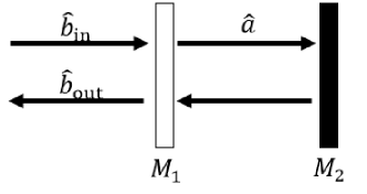
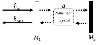
An optical cavity is a system which consists of totally reflecting and/or partially transmitting mirrors [36], [37, Chapter 5.3], [38, Chapter 7], [39]. A widely used type of optical cavities is the so-called Fabry-Perot cavity, as depicted in Fig. 1. In this figure, the electromagnetic filed inside the cavity is mathematically modelled by the bosonic annihilation operator . The right-hand mirror () is totally reflecting, while the left-hand mirror () is partially transmitting. The left-hand mirror () allows the incident light (denoted by its annihilation operator ) to enter into the cavity. After bouncing inside the cavity for a while, the electromagnetic field leaves the cavity from the partially transmitting mirror , and together with the directly reflected light, forms the outgoing electromagnetic field, as represented by in Fig. 1. The coupling between the cavity and the external electromagnetic field is denoted by . Moreover, let the de-tuning between the cavity mode and the carrier frequency of the incident light field be , the dynamics of the Fabry-Parot cavity is, [31, Chapter 5.3], [38, Chapter 7], [36, Section III],
| (8za) | |||||
| (8zb) | |||||
The impulse response function for system is given by
| (8zaa) |
while when . Let be a continuous-mode single-photon Fock state
| (8zab) |
with an exponentially decaying pulse shape
| (8zac) |
The state can describe a single-photon field emitted from an optical cavity with damping rate [38, 3]. Then the input covariance function is
| (8zaf) | |||||
| (8zak) |
On the other hand, by the input-output relation [26], the steady-state output single-photon state has the pulse shape
| (8zal) |
The steady-state output covariance function is
| (8zam) |
By (8v) and (8zak), the Wigner spectrum of the input covariance function can be expressed in terms of both time and frequency
| (8zan) |
Similarly, by (8v) and (8zam), we can get the Wigner spectrum of the output covariance function
| (8zao) |
where
| (8zapa) | |||
| (8zapb) | |||
If we let decay rate , then the following equation holds
| (8zapaq) |
That is, the output single-photon state is identical to the input single-photon state.
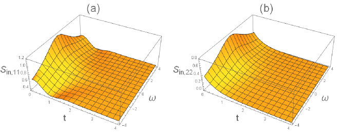
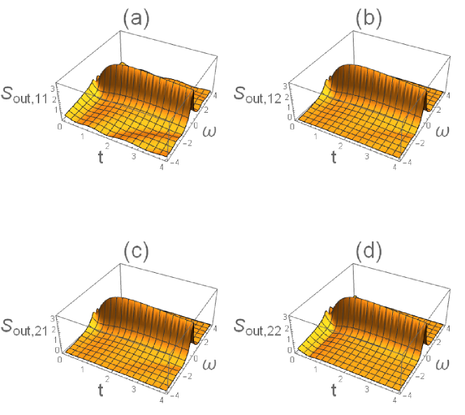
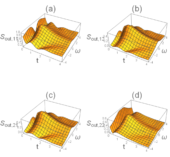
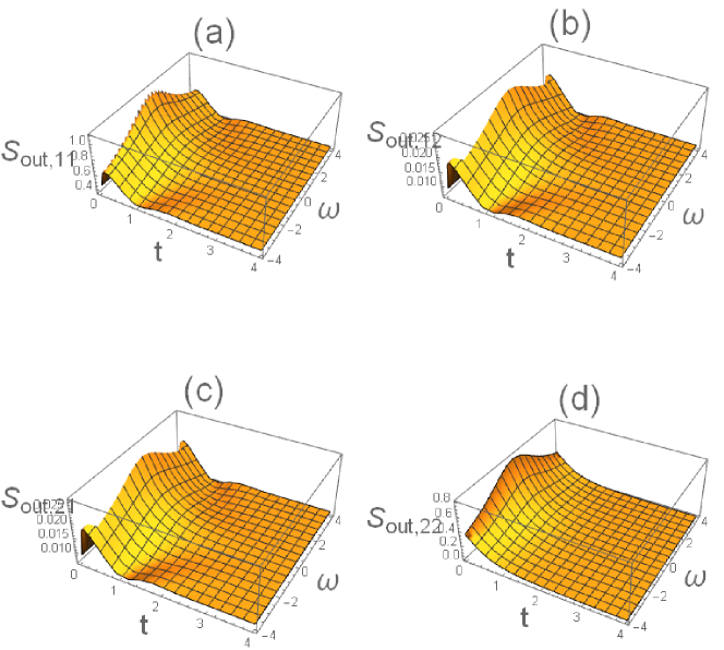
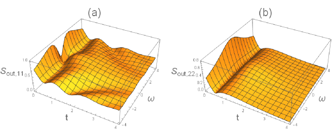
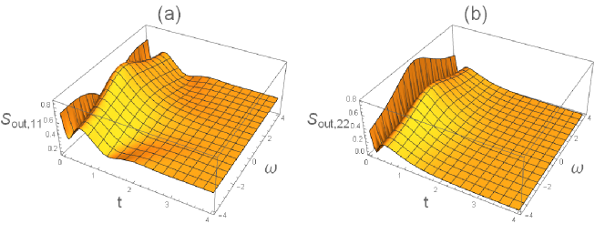
It should be noted that throughout the paper the quantities plotted are all dimensionless. In the following we fix damping rate . In Fig. 2, (a) and (b) are the diagonal entries of the input Wigner spectrum respectively and both of them are exponentially decaying with respect to time . Fig. 3, Fig. 4 and Fig. 5 are the output Wigner spectra with different decay rates and the same de-tuning . Fig. 6, Fig. 7 and Fig. 8 are the output Wigner spectra with same decay rate and different de-tunings .
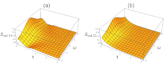
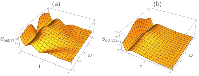
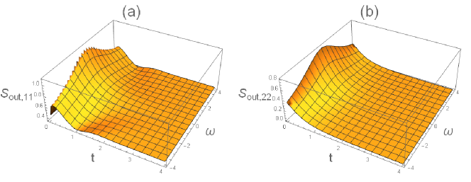
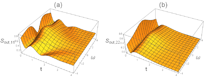
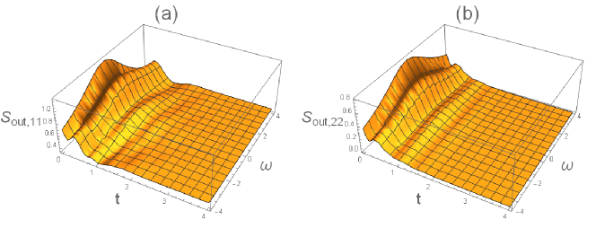
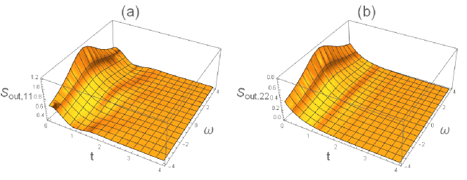
By comparing these figures, we can see that there exist five cases. : the output Wigner spectrum will be close to the input when the decay rate is very small (compare Fig. 2 and Fig. 3); this can be explained by comparing (8zan) and (8zao) directly. : the output Wigner spectrum will also be close to the input when the decay rate is very large (compare Fig. 2 and Fig. 5). Since the impulse response function when , the output state will be close to the input state. : the output Wigner spectrum would be much similar to the input when the de-tuning is very large since the optical cavity has little influence on the photons, see Fig. 8. : it can be seen from Fig. 4 that the output Wigner spectrum is quite different from the input one when is not very large or small. Moreover, (a) (for ) and (b) (for ) are quite different. : The output Wigner spectrum would change a lot with a small de-tuning since there exists a strong interaction between the photon and system (compare Figs. 2 and 6). Therefore, with Wigner spectrum, we are able to observe the changes of the system’s response to the input signals in the time and frequency domains simultaneously. To the best knowledge of the authors, this has not been done before in the single-photon setting.
3 Wigner spectrum for degenerate parametric amplifier
A degenerate parametric amplifier (DPA) is an open oscillator that is able to amplify a quadrature of the cavity mode and produce squeezed output fields, see Fig 9 [31, Chapter 6.3], [38, Chapter 7.6], [37, Chapter 6.3], [39]. A model for a DPA is [31, 26]
| (8zapari) | |||||
| (8zaparj) | |||||
Driven by a single-photon Fock state, the steady output state is no longer a single-photon state because the DPA has pump and the system is not passive any more. The steady output state belongs to the class of photon-Gaussian states which is defined in [26]. Let the single-photon input Fock state be that defined in (8zac). The output covariance function is
| (8zaparas) |
whose Wigner spectrum is
| (8zaparat) |
Here, the explicit forms of output covariance function and Wigner spectrum are given in A. Similar with the cavity case, if we let decay rate , (8zapaq) also holds for the DPA case, which is consistent with the simulation result in Fig. 12.
In the following we fix , . The input Wigner spectrum is as same as the optical cavity case in Fig. 2. Figs. 10-12 are simulation results for different decay rates , where , , , are the entries for the output Wigner spectrum in (8zaparat) respectively. Compared with the cavity case, there exists non-zero off-diagonal parts since DPA is a non-passive system. Moreover, it can be seen clearly from Figs. 10 and 11 that the photon-Gaussian state is significantly different from the single-photon state. A photon-Gaussian state is obtained by driving a DPA with a single-photon state, [26]. Intuitively, a photon-Gaussian state is of the form in which is a pulse shape and is a coherent state. Clearly, when , we get a single-photon Fock state.
An optical cavity is a passive system while a DPA is not. By comparing figures for the cavity case and the DPA case, it can be seen that the Wigner spectrum is able to demonstrate such fundamental difference very clearly in terms of the statistical characterization of the input-output relation.
4 Photon pulse shape engineering
In this section, we will discuss how to engineer photon pulse shapes by means of coherent control methods, namely direct coupling (Fig. 14) and coherent feedback (Fig. 15).
4.1 Direct couplings
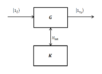
In Fig. 14, two independent systems and may interact by exchanging energy. This energy exchange can be described by an interaction Hamiltonian with the form
| (8zaparau) |
where and are operators on system and respectively. We can denote the directly coupled system by , see [40, 41].
Quantum markovian systems can be conveniently described by the triple formalism, in which is the scattering operator matrix, is the coupling between the system and its environment, and denotes the initial system Hamiltonian, see [42, 43, 44].
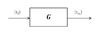
Fig. 13 is an optical cavity with the following parameters,
| (8zaparav) |
where is the system decay rate and denotes the de-tuning for system . is the single-photon input Fock state and is the output state. In Fig. 14, the system is directly coupled with another quantum system with parameters
| (8zaparaw) |
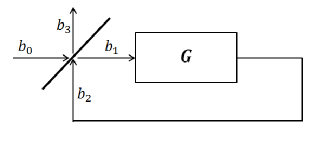
where denotes the de-tuning for system . In this case, the output state is described by . Alternatively, we may use a beamsplitter to form a coherent feedback system, see Fig. 15. In the following, we will derive the explicit forms of output pulse shapes in the frequency domain.
4.2 Photon shape synthesis
Let the pulse shape of a single-photon input Fock state be
| (8zaparaz) |
where is the damping rate. By the Fourier transform, we can get the input pulse shape in the frequency domain
| (8zaparba) |
The transfer function for the original system is given by
| (8zaparbb) |
and the output pulse shape in the frequency domain is
| (8zaparbc) |
Secondly, for the directly coupled system in Fig. 14, we assume that , and . The interaction Hamiltonian is given by
| (8zaparbd) |
Then the Hamiltonian for the whole system is
| (8zaparbe) |
where , .
We get the pulse shape of the output single-photon Fock state for the system , which is
| (8zaparbf) |
4.3 Photon distribution
For the single-photon Fock state we defined before
| (8zaparbi) |
is the creation operator and is the pulse shape which is also known as temporal wave packet. denotes the probability of finding the photon (detection probability) in the interval . In this subsection, we will focus on how the system parameters change the detection probabilities in the control schemes discussed above.
By the inverse Fourier transform, we can get the output temporal wave packets
| (8zaparbj) |
where denotes the -th case we discussed before.
For the direct coupling scheme, Fig. 14, we fix , , . Fig. 16 and Fig. 17 are the detection probabilities for different and respectively. For the coherent feedback control case Fig. 15, detection probabilities for different beamsplitter parameter are given in Fig. 18.
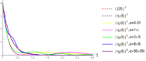
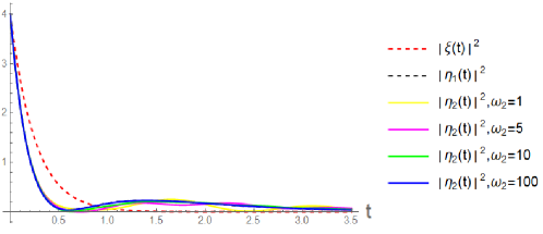
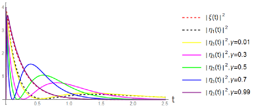
By comparing these three cases, it can be easily seen that the linear quantum feedback network in Fig. 15 has much more influence on the detection probability than the directly coupled system. In addition, the changes of output Wigner spectrum with beamsplitter parameter for quantum feedback network also have been analyzed. In Fig. 19 - Fig. 21, let the decay rate of the optical cavity be and damping rate be , it can be verified that those changes are consistent with the photon distributions in Fig. 18.

On the other hand, we assume the system for the feedback network in Fig. 15 is a DPA with the triple parameters
| (8zaparbk) |
Then the whole feedback network system parameters with beamsplitter are given by
| (8zaparbl) |
So the only change between the feedback network and the original system is . There exist three cases as follows:
1) , the feedback network reduces to the open-loop system .
2) , then , , there is no interaction between field and system.
3) , , the decay rate is always enhanced. However, it is clear that
| (8zaparbm) |
Therefore, by tuning the beamsplitter we can get various output single-photon states. It is worth noting that the same feedback scheme Fig. 15 has been used for optical squeezing, see theoretical [45] and experimental [46].
5 Conclusion
In this article, the Wigner spectrum has been used to analyze the statistical properties of continuous-mode single-photon Fock states. The Wigner spectrum is able to show the significant difference between the statistical nature of the output fields of an optical cavity and a degenerate parametric amplifier (DPA), driven by a continuous-mode single-photon Fock state. Several control schemes are compared for photon pulse-shaping. It has been demonstrated that the coherent feedback control scheme is very effective in photon pulse-shaping.
References
- [1] Beveratos A, Brouri R, Gacoin T, Villing A, Poizat J P and Grangier P 2002 Physical Review Letters 89 187901
- [2] Gisin N and Thew R 2007 Nature photonics 1 165–171
- [3] Loudon R 2000 The quantum theory of light (Oxford university press)
- [4] Knill E, Laflamme R and Milburn G J 2001 nature 409 46–52
- [5] Giovannetti V, Lloyd S and Maccone L 2004 Science 306 1330–1336
- [6] Giovannetti V, Lloyd S and Maccone L 2011 Nature Photonics 5 222
- [7] Leroux I D, Schleier-Smith M H, Zhang H and Vuletić V 2012 Physical Review A 85 013803
- [8] Moehring D, Maunz P, Olmschenk S, Younge K, Matsukevich D, Duan L M and Monroe C 2007 Nature 449 68
- [9] Kimble H J 2008 Nature 453 1023
- [10] Aghamalyan D and Malakyan Y 2011 Physical Review A 84 042305
- [11] Blow K, Loudon R, Phoenix S J and Shepherd T 1990 Physical Review A 42 4102
- [12] Braunstein S L and Van Loock P 2005 Reviews of Modern Physics 77 513
- [13] Furusawa A and Van Loock P 2011 Quantum teleportation and entanglement: a hybrid approach to optical quantum information processing (John Wiley & Sons)
- [14] Brecht B, Reddy D V, Silberhorn C and Raymer M G 2015 Physical Review X 5 041017
- [15] Garrison J and Chiao R 2008 Quantum optics (Oxford University Press)
- [16] Milburn G 2008 The European Physical Journal Special Topics 159 113
- [17] Ogawa H, Ohdan H, Miyata K, Taguchi M, Makino K, Yonezawa H, Yoshikawa J i and Furusawa A 2016 Physical Review Letters 116 233602
- [18] Wang Y, Minář J, Sheridan L and Scarani V 2011 Physical Review A 83 063842
- [19] Gough J E, James M R and Nurdin H I 2011 50th IEEE Conference on Decision and Control and European Control Conference 5570–5576
- [20] Gough J E, James M R, Nurdin H I and Combes J 2012 Physical Review A 86 043819
- [21] Gough J E, James M R and Nurdin H I 2013 Quantum information processing 12 1469
- [22] Baragiola B Q, Cook R L, Brańczyk A M and Combes J 2012 Physical Review A 86 013811
- [23] Song H, Zhang G and Xi Z 2016 SIAM Journal on Control and Optimization 54 1602–1632
- [24] Carvalho A, Hush M and James M 2012 Physical Review A 86 023806
- [25] Gheri K M, Ellinger K, Pellizari T and Zoller P 1998 Fortschritte der Physik 46 401–416
- [26] Zhang G and James M R 2013 Automatic Control, IEEE Transactions on 58 1221
- [27] Yamamoto N and James M R 2014 New Journal of Physics 16 073032
- [28] Qin Z, Prasad A S, Brannan T, MacRae A, Lezama A and Lvovsky A 2015 Light: Science & Applications 4 e298
- [29] Munro W, Nemoto K and Milburn G 2010 Optics Communications 283 741–746
- [30] Pan Y, Zhang G and James M R 2016 Automatica 69 18–23
- [31] Gardiner C and Zoller P 2004 Quantum noise: a handbook of Markovian and non-Markovian quantum stochastic methods with applications to quantum optics vol 56 (Springer Science & Business Media)
- [32] Gough J E 2005 Russian Journal of Mathematical Physics 10 142–148
- [33] Wigner E 1932 Physical Review 40 749
- [34] Ville J d et al. 1948 Cables et transmission 2 61–74
- [35] Sandsten M 2013 Time-Frequency Analysis of Non-Stationary Processes (Lund University, Centre for Mathematical Sciences)
- [36] Yanagisawa M and Kimura H 2003 IEEE Transactions on Automatic control 48 2107–2120
- [37] Bachor H A and Ralph T C 2004 A guide to experiments in quantum optics (Wiley)
- [38] Walls D F and Milburn G J 2007 Quantum optics (Springer Science & Business Media)
- [39] Nurdin H I, James M R and Doherty A C 2009 SIAM Journal on Control and Optimization 48 2686–2718
- [40] Wiseman H M and Milburn G J 1994 Physical review A 49 4110
- [41] Zhang G and James M R 2011 Automatic Control, IEEE Transactions on 56 1535
- [42] Gough J and James M R 2009 Automatic Control, IEEE Transactions on 54 2530
- [43] Gough J E, James M and Nurdin H 2010 Physical Review A 81 023804
- [44] Zhang G and James M R 2012 Chinese Science Bulletin 57 2200
- [45] Gough J E and Wildfeuer S 2009 Physical Review A 80 042107
- [46] Iida S, Yukawa M, Yonezawa H, Yamamoto N and Furusawa A 2012 Automatic Control, IEEE Transactions on 57 2045
Appendix A The explicit form of output Wigner spectrum for DPA
If the single-photon input has the pulse shape defined in (8zac), we can get the pulse shape of output state
Then, the output covariance function is
where
| (8zaparbr) | |||||
| (8zaparbv) | |||||
| (8zaparbw) | |||||
| (8zaparca) |
Thus, the Wigner spectrum of output covariance function for the DPA is
| (8zaparcd) |
where