On the spatio-temporal behavior of magnetohydrodynamic turbulence in a magnetized plasma

Abstract

Using direct numerical simulations of three-dimensional magnetohydrodynamic (MHD) turbulence the spatio-temporal behavior of magnetic field fluctuations is analyzed. Cases with relatively small, medium and large values of a mean background magnetic field are considered. The (wavenumber) scale dependent time correlation function is directly computed for different simulations, varying the mean magnetic field value. From this correlation function the time decorrelation is computed and compared with different theoretical times, namely, the local non-linear time, the random sweeping time, and the Alfvénic time, the latter being a wave effect. It is observed that time decorrelations are dominated by sweeping effects, and only at large values of the mean magnetic field and for wave vectors mainly aligned with this field time decorrelations are controlled by Alfvénic effects.

I Introduction

It is known that in the linear approximation the magnetohydrodynamic (MHD) equations can sustain Alfvén waves. The simplest case corresponds to incompressible MHD with a uniform background magnetic field ${\bf B_{0}}$, for which the linear dispersion relation (in the ideal non-dissipative case) describes waves with frequency $w={\bf k}\cdot{\bf v_{A}}$, for wavevector ${\bf k}$, Alfvén velocity ${\bf v_{A}}={\bf B_{0}}/\sqrt{4\pi\rho}$, and density $\rho$. Also, the complex Fourier components of the velocity ${\bf v}({\bf k})$ and of magnetic field fluctuations ${\bf b}({\bf k})$ are transverse to the wavevector, i.e., ${\bf v}({\bf k})\cdot{\bf k}={\bf b}\cdot{\bf k}=0$. Interestingly, these waves when considered in isolation are exact nonlinear solutions of the MHD equations.

However, when non-linear terms are taken into account, the system can also develop far from equilibrium dynamics, with the waves coexisting with eddies in a fully developed turbulent flow dmitruk_waves_2009 . In this turbulent regime one does not necessarily expect a direct or explicit relation between frequency and wavenumber, such as the dispersion relation for waves. This regime is characterized by interactions of several types, such as local-in-scale nonlinear distortion of eddies monin_statistical_2013 ; kolmogorov_local_1941 ; mccomb_physics_1992 , and non-local effects alexakis_turbulent_2007 ; alexakis_anisotropic_2007 ; teaca_energy_2009 ; mininni_scale_2011 the most extreme of which is transport or “sweeping” of small eddies by large eddies kraichnan_structure_1959 ; tennekes_eulerian_1975 ; chen_sweeping_1989 ; nelkin_time_1990 . Furthermore, for MHD turbulence pouquet_strong_1976 ; zhou_magnetohydrodynamic_2004 , in addition to the global nonlinear time $\tau_{nl}$, there are also time scales associated with scale-dependent (local) nonlinear effects, nonlocal sweeping, and wave propagation zhou_magnetohydrodynamic_2004 .

In the early 70’s, investigation of hydrodynamic turbulence was directed to study the decorrelation time of the velocity field orszag_numerical_1972 ; orszag_analytical_1970 ; tennekes_eulerian_1975 ; heisenberg_zur_1948 ; comte-bellot_simple_1971 . The main conclusion was that the sweeping dominates the temporal decorrelation in the inertial range zhou_non-gaussian_1993 ; sanada_random_1992 . Recently, a similar study has been implemented in magnetohydrodynamics servidio_time_2011 ; matthaeus_eulerian_2010 ; carbone_anisotropy_2011 . One difference with the hydrodynamic case is the presence of other non-local phenomena (besides the sweeping), such as the Alfvénic propagation or Alfvénic distortion, namely “magnetic sweeping”. The main result of Servidio et al. servidio_time_2011 on the temporal decorrelation for isotropic turbulence was that, as in hydrodynamics, the temporal decorrelation in MHD is governed by nonlocal interactions (in this case, sweeping and Alfvén decorrelation). However, they were not able to distinguish between the effect of sweeping and Alfvénic distortion. In this paper, our main objective is to extend this analysis and generalize it to magnetized plasmas at large scales where the MHD approximation is valid.

In this work we study the different decorrelation times through the various scales in the inertial range for MHD turbulence with a guide field. The main objective is to understand the temporal decorrelation of the fluctuations, by studying the relative value of decorrelation times for the different scales. Thus, we will be able to relate the scaling laws of the decorrelation times with the different contributing physical effects: non-linear distorsion, random sweeping and Alfvén wave propagation. In other words, we will study the characteristic memory timescale for each spatial scale, in order to identify the mechanisms of temporal decorrelation and to see whether they are local or non-local. For this purpose, we will consider the fluctuations at more than one length scale, to discern between the different phenomena that are associated with temporal decorrelation, in particular Alfvén wave propagation and random sweeping. This method, based on the computation of spatio-temporal spectra and on correlation functions, was proposed and implemented in rotating fluids by Clark di Leoni et al. clark_di_leoni_quantification_2014 (see also clark_di_leoni_spatio-temporal_2015 for a general description of the method). Meyrand and Galtier recently used the spatio-temporal spectrum to study the transition from weak to strong turbulence in MHD meyrand_direct_2016 , and intermittency in weak MHD turbulence meyrand_weak_2015 . Here we consider the strong turbulent regime, and compute both spectra as well as decorrelation times.

II Equations and numerical simulations

II.1 The MHD equations

The incompressible MHD equations (momentum and induction equations) in dimensionless units are

$$\frac{\partial{\bf v}}{\partial t}+{\bf v}\cdot\nabla{\bf v}=-\frac{1}{\rho}\nabla p+{\bf j}\times{\bf B}+\frac{1}{R}\nabla^{2}{\bf v},$$ (1)

$$\frac{\partial{\bf b}}{\partial t}=\nabla\times({\bf v}\times{\bf B})+\frac{1}{R_{m}}\nabla^{2}{\bf b},$$ (2)

where ${\bf v}$ is the plasma velocity; ${\bf B}={\bf b}+{\bf B_{0}}$ the magnetic field, with a fluctuating part ${\bf b}$ and a mean DC field ${\bf B_{0}}=B_{0}\hat{\mathbf{x}}$; ${\bf j}=\nabla\times{\bf b}$ the current density; $p$ the pressure, and $\rho$ the plasma density. The units are based on a characteristic speed $v_{0}$, which for MHD is chosen to be the typical Alfvén speed of the magnetic field fluctuations, $v_{0}=\sqrt{\langle b^{2}\rangle/(4\pi\rho)}$, where $\langle.\rangle$ denotes a spatial average. The dimensionless parameters appearing in the equations are the kinetic and magnetic Reynolds numbers, $R=v_{0}L/\nu$ and $R_{m}=v_{0}L/\mu$ respectively, with $\nu$ the kinematic viscosity, $\mu$ the magnetic diffusivity and $L$ the characteristic length scale (the simulation box side length is defined as $2\pi L$). The unit time is $t_{0}=L/v_{0}$, which for MHD becomes the Alfvén crossing time based on magnetic field fluctuations.

II.2 Wavenumber-frequency spectrum and correlation functions

From Eqs. (1-2) and simple scaling arguments, one can estimate different characteristic times. The local eddy turnover time can be defined as $\tau_{nl}\sim\left[kv(k)\right]^{-1}$, where $k$ is the wave number and $v(k)$ is the amplitude of velocity due to fluctuations at scale $\sim 1/k$. For a Kolmogorov-type prediction of the velocity scaling, $v\sim v_{rms}\left(kL\right)^{-1/3}$, the nonlinear time scales in the inertial range can be approximately written as $\tau_{nl}=C_{nl}\left[v_{rms}L^{-1/3}\left(\sqrt{k^{2}_{\perp}+k^{2}_{\parallel}}\right)^{2/3}\right]^{-1}$, where $C_{nl}$ is a dimensionless constant of order unity. In the latter, $v_{rms}=\left\langle|{\bf v}|^{2}\right\rangle^{1/2}$ is a global quantity, typically dominated by contributions from the large scales.

The physics of time decorrelation depends on other effects and therefore other available MHD time scales. One example is the sweeping characteristic time at scale $\sim 1/k$, which may be expressed as $\tau_{sw}=C_{sw}\left(v_{rms}\sqrt{k^{2}_{\perp}+k^{2}_{\parallel}}\right)^{-1}$. This time corresponds to the advection of small scale structures by the large scale flow. Analogously, a characteristic Alfvén time can be defined as $\tau_{A}=C_{A}\left(B_{0}k_{\parallel}\right)^{-1}$. Here, $C_{sw}$ and $C_{A}$ are other dimensionless constants of order unity. All these timescales depend on the wave vector, and assuming the shortest timescale dominates the dynamics, different regions in $k$-space in the energy spectrum can be defined.

The statistics of, for example, the magnetic field may be characterized by the spatio-temporal two-point autocorrelation function

$$R({\bf r},\tau)=\left\langle{\bf b}({\bf x},t)\cdot{\bf b}({\bf x}+{\bf r},t+\tau)\right\rangle/\left\langle{\bf b}^{2}\right\rangle.$$ (3)

Note that this expression contains both the energy spectrum and the Eulerian frequency spectrum (Wiener-Khinchin theorem); however, it contains much more information which allows us to make a more subtle analysis of the spatio-temporal relations. Fourier transforming in $r$ leads to a time-lagged spectral density which may be further factorized as $S({\bf k},\tau)=S({\bf k})\Gamma({\bf k},t)$, where ${\bf k}$ is the wave vector. The function $\Gamma({\bf k},\tau)$, the scale-dependent (or filtered) correlation function heisenberg_zur_1948 ; comte-bellot_simple_1971 ; orszag_numerical_1972 , represents the dynamical decorrelation effects describing the time decorrelation of each spatial mode ${\bf k}$.

The function $\Gamma({\bf k},\tau)$ is thus the temporal correlation function of the Fourier mode ${\bf k}$. Using this, we will be able to identify the characteristic decorrelation time for each mode ${\bf k}$ and therefore the loss of memory of 3D-fluctuations whose characteristics lengths are of order $k_{x}^{-1}$, $k_{y}^{-1}$ and $k_{z}^{-1}$. When there is no guide field we usually expect the flow to be isotropic both in real space and in Fourier space, and therefore it is sufficient to study the function $\Gamma(k,\tau)$ that depends only on $k=|{\bf k}|$. On the other hand, in the presence of a guide field, the turbulence is anisotropic; therefore, it is reasonable to use $\Gamma=\Gamma(k_{\perp},k_{\parallel},\tau)$ where $k_{\perp}$ and $k_{\parallel}$ are the perpendicular and parallel (to the mean magnetic field) Fourier wave numbers.

The function $\Gamma(k_{\perp},k_{\parallel},\tau)$ can help us to understand the dynamics of different regions in Fourier space. For example, the function $\Gamma(k_{\perp}=0,k_{\parallel},\tau)$ give us information about fluctuations that vary only in the parallel direction. In the same way $\Gamma(k_{\perp},k_{\parallel}=0,\tau)$ gives information about fluctuations that vary only in the perpendicular direction. Also of interest is the information obtained from the $\Gamma(k_{\perp}=k_{0},k_{\parallel},\tau)$ and the $\Gamma(k_{\perp},k_{\parallel}=k_{0},\tau)$ functions, when one of the Fourier wavenumbers (the parallel or the perpendicular) is set to a fixed value $k_{0}$. For example, studying the decorrelation time for $\Gamma(k_{\perp}=k_{0},k_{\parallel},\tau)$ as a function of $k_{\parallel}$ would be useful to see the memory loss over time of fluctuations whose perpendicular characteristic length is $\sim k_{0}^{-1}$ (a fixed selected length), as a function of its parallel scale $\sim k_{\parallel}^{-1}$. This would give us information on two important issues: how the memory in one direction affects the other, and more importantly, how to distinguish between random sweeping and Alfvén propagation.

II.3 Numerical simulations

We use a standard pseudospectral code to solve numerically the incompressible three-dimensional MHD equations with a guide field gomez_parallel_2005 ; gomez_mhd_2005 . All results reported here are from runs with resolution of $N^{3}=512^{3}$ grid points. A second-order Runge-Kutta time integration scheme is used. We use weak, moderate and strong external magnetic fields, $B_{0}=0.25$, $1$ and $8$ (in units of the initial r.m.s. magnetic fluctuations value). We also consider the case $B_{0}=0$ for reference with previous studies servidio_time_2011 . Periodic boundary conditions are assumed in all directions of a cube of side $2\pi L$ (where $L=1$ is the initial correlation length of the fluctuations, defined as the unit length). Aliasing is removed by a two-thirds rule truncation method. The initial state consists of nonzero amplitudes for the ${\bf v}({\bf k})$ and ${\bf b}({\bf k})$ fields, equipartioned in the wave numbers within shells $1.1\leq k\leq 4$, with $k=|{\bf k}|$ (in units of $2\pi L/\ell$ with $\ell$ the wavelength). Random phases have been chosen for both fields. To achieve a statistically steady state we consider a driving which consists of forcing terms added to Eqs. (1-2) in a fixed set of Fourier modes in the band $0.9\leq k\leq 1.8$. The forcing has a random and a time-coherent component, so that the correlation time of the forcing is $\tau_{f}\approx 1$ (of the order of the unit time $t_{0}$).

The temporal range used to analyze the results is over $20$ unit times for $B_{0}=0$ and $B_{0}=0.25$, over $25$ unit times for $B_{0}=1$, and over $10$ unit times for $B_{0}=8$. All these time spans are considered after the system reached a turbulent steady state, and we verified that they were enough to ensure convergence of spectra and correlation functions.

III Results

III.1 Energy spectra and dominant time scales

The axisymmetric energy spectrum $e(|\mathbf{k_{\perp}}|=\sqrt{k_{y}^{2}+k_{z}^{2}},k_{\parallel}=k_{x},t)$, defined as

$$\begin{split}e(k_{\perp},k_{\parallel},t)=\sum_{\begin{subarray}{c}k_{\perp}\leq|\mathbf{k}\times\hat{\mathbf{x}}|<k_{\perp}+1\\ k_{\parallel}\leq k_{x}<k_{\parallel}+1\end{subarray}}|\hat{\mathbf{u}}(\mathbf{k},t)|^{2}+|\hat{\mathbf{b}}(\mathbf{k},t)|^{2}=\\ =\int\left(|\hat{\mathbf{u}}(\mathbf{k},t)|^{2}+|\hat{\mathbf{b}}(\mathbf{k},t)|^{2}\right)|\mathbf{k}|\sin\theta_{k}~{}d\phi_{k},\end{split}$$ (4)

provides information on the anisotropy of the turbulence relative to the the guide field mininni_isotropization_2012 . In this study, the guide field is chosen along the $x$ axis, and thus the wave vector components $k_{\parallel}$ and $k_{\perp}$, and the polar angles in Fourier space $\theta_{k}$ and $\phi_{k}$, are relative to this axis. In other words, in Eq. (4) $\theta_{k}=\arctan(k_{\perp}/k_{\parallel})$ is the co-latitude in Fourier space with respect to the axis with unit vector $\hat{\mathbf{x}}$ (that is, in the direction of the guide field), and $\phi_{k}$ is the longitude with respect to the $y$-axis. The first expression involving the summation in Eq. (4) is the definition of the axisymmetric energy spectrum for a discrete Fourier space (i.e., as used in the simulations), while the second expression with the integral corresponds to the continuum limit. In the following we treat both expressions as equivalent, replacing integrals by summations when required for the numerics.

From the axisymmetric spectrum above, one can define the time averaged reduced perpendicular energy spectrum $E(k_{\perp})$ mininni_isotropization_2012 as

$$E\left(k_{\perp}\right)=\frac{1}{T}\int\int e(|\mathbf{k_{\perp}}|,k_{\parallel},t)\,dk_{\parallel}~{}dt,$$ (5)

where we integrated over parallel wave numbers to obtain a spectrum that depends only on $k_{\perp}$. Equivalently, the isotropic energy spectrum $E(k)$ can be obtained from Eq. (4) by integrating over $\theta_{k}$ in Fourier space. Figure 1 shows the isotropic energy spectrum $E(k)$ for the run with $B_{0}=0$, and the reduced perpendicular energy spectrum $E(k_{\perp})$ for the runs with non-zero guide field.

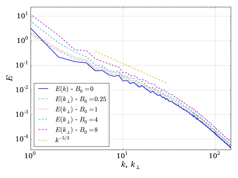
Figure 1: Reduced perpendicular energy spectra $E(k_{\perp})$ for the simulations with $B_{0}=0.25$, $1$, $4$, and $8$, and isotropic energy spectrum $E(k)$ for the simulation with $B_{0}=0$. Kolmogorov scaling, $\sim k_{\perp}^{-5/3}$, is shown as reference.

Figure 2 shows contour plots of $e(k_{\perp},k_{\parallel})/\sin(\theta_{k})$, that is, the axisymmetric spectrum (averaged in time), for the runs with $B_{0}=0$, $B_{0}=0.25$, $B_{0}=1$, $B_{0}=4$, and $B_{0}=8$ respectively. For an isotropic flow ($B_{0}=0$, see Fig. 2), contours of $e(k_{\perp},k_{\parallel})/\sin(\theta_{k})$ are circles as expected mininni_isotropization_2012 . As the guide field intensity increases, energy becomes more concentrated near the axis with $k_{\parallel}=0$, evidencing the formation of elongated structures in the direction of the guide field (or, in other words, of the relative decrease of parallel gradients of the fields with respect to perpendicular gradients).

The characteristic times defined in the Introduction, $\tau_{A}$, $\tau_{sw}$, and $\tau_{nl}$, divide the Fourier space in Fig. 2 in regions depending on how the time scales are ordered:

$$\tau_{A}<\tau_{sw}\hskip 1.42271pt\Rightarrow\hskip 1.42271ptk_{\perp}<\left(\sqrt{\left(\frac{B_{0}}{v_{rms}}\right)^{2}\cdot\left(\frac{C_{sw}}{C_{A}}\right)^{2}-1}\right)k_{\parallel},$$ (6)

$$\tau_{A}<\tau_{nl}\hskip 1.42271pt\Rightarrow\hskip 1.42271ptk_{\perp}<\left(\sqrt{\left(\frac{B_{0}}{v_{rms}}\right)^{3}\left(\frac{C_{nl}}{C_{A}}\right)^{3}Lk_{\parallel}-1}\right)k_{\parallel},$$ (7)

$$\tau_{nl}<\tau_{sw}\hskip 1.42271pt\Rightarrow\hskip 1.42271pt\left(k_{\perp}^{2}+k_{\parallel}^{2}\right)^{1/6}<\frac{C_{sw}}{C_{nl}L^{1/3}}.$$ (8)

In Figure 2 we indicate the curves corresponding to the modes that satisfy the relations $\tau_{A}\lesssim\tau_{sw}$ and $\tau_{A}\lesssim\tau_{nl}$, respectively for $B_{0}=0$, $0.25$, $1$, $4$, and $8$ (assuming, to plot all curves, that $C_{sw}\approx C_{nl}\approx C_{A}\approx 1$; this choice will be later confirmed by the analysis of the correlation functions).

As we can see from Eq. (8), the region where $\tau_{nl}\leq\tau_{sw}$ is a small circle around the origin, where $k_{\perp}^{2}+k_{\parallel}^{2}\leq(C_{sw}/L^{1/3}C_{nl})^{6}\approx 1$, and is not shown in the figure. Modes outside the region with $\tau_{nl}<\tau_{sw}$ should decorrelate with the sweeping time or the Alfvén time, depending on which one is fastest. Equation (6) tells us that in the area to the left of the curve $\tau_{A}\sim\tau_{sw}$ we have $\tau_{A}<\tau_{sw}$, while Eq. (7) tells us that in the area to the left of the curve $\tau_{A}\sim\tau_{nl}$ we have $\tau_{A}<\tau_{nl}$ (see Fig. 2d). For the largest value of $B_{0}$ considered (i.e., the simulation with $B_{0}=8$), most of the modes have the Alfvén period as the fastest time (i.e., the largest area in the plot is above and to the left of the curve $\tau_{A}\sim\tau_{sw}$), although a significant fraction of the energy in the system is not in these modes as it concentrates instead near the axis with $k_{\parallel}=0$.

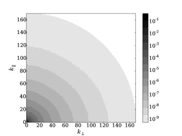
(a) $B_{0}=0$

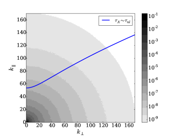
(b) $B_{0}=0.25$

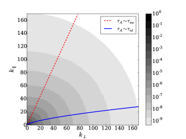
(c) $B_{0}=1$

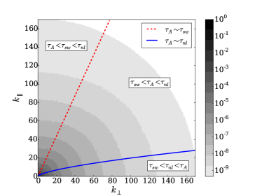
(d) $B_{0}=1$ with explanation

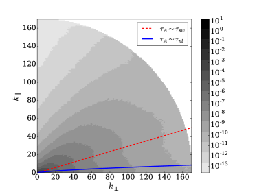
(e) $B_{0}=4$

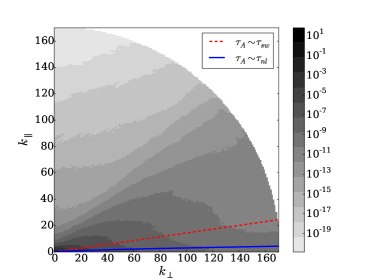
(f) $B_{0}=8$

Figure 2: Isocontours of the axisymmetric energy spectrum $e(k_{\perp},k_{\parallel})$ for different values of $B_{0}$. Dark means larger energy density (in logarithmic scale). The lines indicate the modes for which sweeping time or local non-linear time become equal to the Alfvén time. For large $B_{0}$ the isocontours change shape as they cross each of these lines. Note also the stronger anisotropy of the spectrum as $B_{0}$ increases, as well as the increase in the surface covered by modes which have the Alfvén period as the fastest time.

III.2 Spatio-temporal spectra

Figure 3 (for the simulation with $B_{0}=0.25$), Fig. 4 ($B_{0}=1$), and Fig. 5 ($B_{0}=8$) show the wave vector and frequency spectrum $E(\mathbf{k},\omega)/E(\mathbf{k})$ for modes $\mathbf{k}$ with $k_{\perp}=0$, where

$$E(\mathbf{k})=\int E(\mathbf{k},\omega)d\omega$$ (9)

is the total energy spectrum. With this choice for the normalization, the frequencies that concentrate most of the energy for each $\mathbf{k}$ are more clearly visible. For $B_{0}=0.25$ (Fig. 3) we observe a spread of the energy concentration clearly below the sweeping relation line (i.e., we see excitations in all modes with frequency equal or smaller than $\omega=v_{rms}k_{\parallel}$, indicating small scale structures are advected by all velocities equal and smaller than $v_{rms}$). A weak accumulation near the Alfvénic dispersion relation $\omega=B_{0}k_{\parallel}$ is also visible for small wavenumbers $k_{\parallel}$, although the broad spectrum (in the frequency domain) suggests sweeping is dominant in this case.

As the mean field increases to $B_{0}=1$ (Fig. 4), some of the energy is concentrated above the sweeping line and starts to follow the Alfvénic dispersion relation, although the spectrum is still broad in frequencies, with a large fraction of the energy below the sweeping relation. This behavior changes drastically for larger values of $B_{0}$. In Figure 5 ($B_{0}=8$) we can see energy clearly concentrating around the dispersion relation of Alfvén waves, with the power sharply peaked around the wave modes up to $k_{\parallel}\approx 10$, and then suddenly broadening towards the sweeping relation for larger wavenumbers. Note that this indicates a competition between the magnetohydrodynamic sweeping time and the Alfvén time, with the former becoming dominant at large scales for large values of $B_{0}$. These results support and enhance the ones obtained by Dmitruk and Matthaeus dmitruk_waves_2009 , and are compatible for small wavenumber and large $B_{0}$ with those recently obtained in meyrand_direct_2016 ; meyrand_weak_2015 . In particular, meyrand_direct_2016 also reported a transition from a narrow wave spectrum to a broader spectrum, although the scale and mechanism responsible for the transition was not clear. As will be confirmed next from the correlation functions, the competition between sweeping and the Alfvén time as the dominant decorrelation time is responsible for the change observed in the behavior of the spectrum.

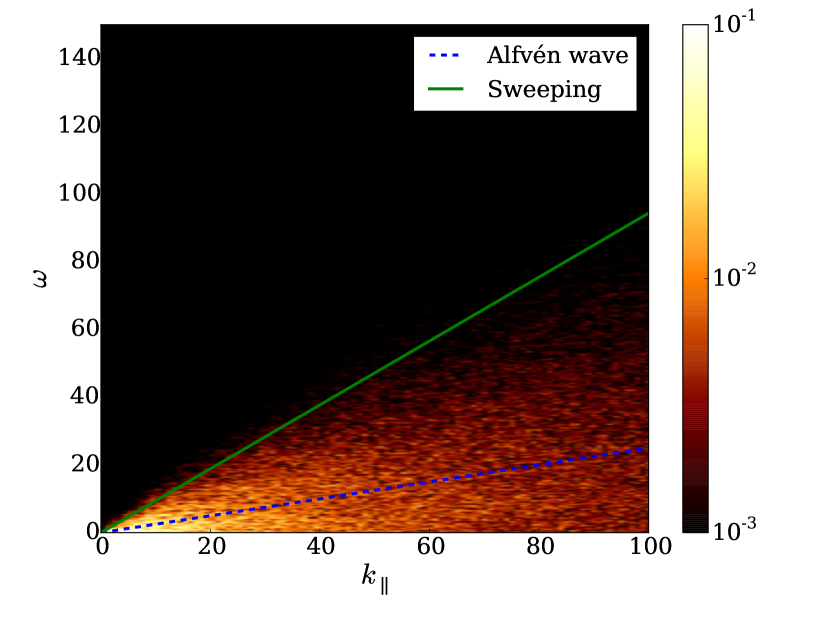
Figure 3: Normalized wave vector and frequency spectrum $E({\bf k},\omega)/E({\bf k})$ for the run with ${\bf B_{0}}=0.25$, for modes with $k_{\perp}=0$, and thus as a function of $k_{\parallel}$. Lighter regions indicate larger energy density. The spectrum corresponds to the power in the time and space Fourier transform of the fields, such that accumulation of energy in modes near the dispersion relation (or in all modes below the sweeping curve) indicates dominance of a physical effect (i.e., of its associated frequency) in the dynamics of a given scale $\sim 1/k_{\parallel}$. The dashed (blue) line indicates the dispersion relation for Alfvén waves, and the continuous (green) line indicates the sweeping relation. A broad excitation of modes is observed for all modes with $\omega\leq v_{rms}k_{\parallel}$ (sweeping), while only a very weak accumulation at small $k_{\parallel}$ can be seen for $\omega=B_{0}k_{\parallel}$ (Alfvén).

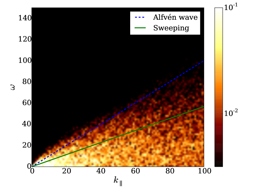
Figure 4: Normalized wave vector and frequency spectrum $E({\bf k},\omega)/E({\bf k})$ for the run with $B_{0}=1$, for modes with $k_{\perp}=0$, and thus as a function of $k_{\parallel}$ and $\omega$. Lighter regions indicate larger energy density. The dashed (blue) line indicates the dispersion relation for Alfvén waves and the continuous (green) line indicates the sweeping relation.

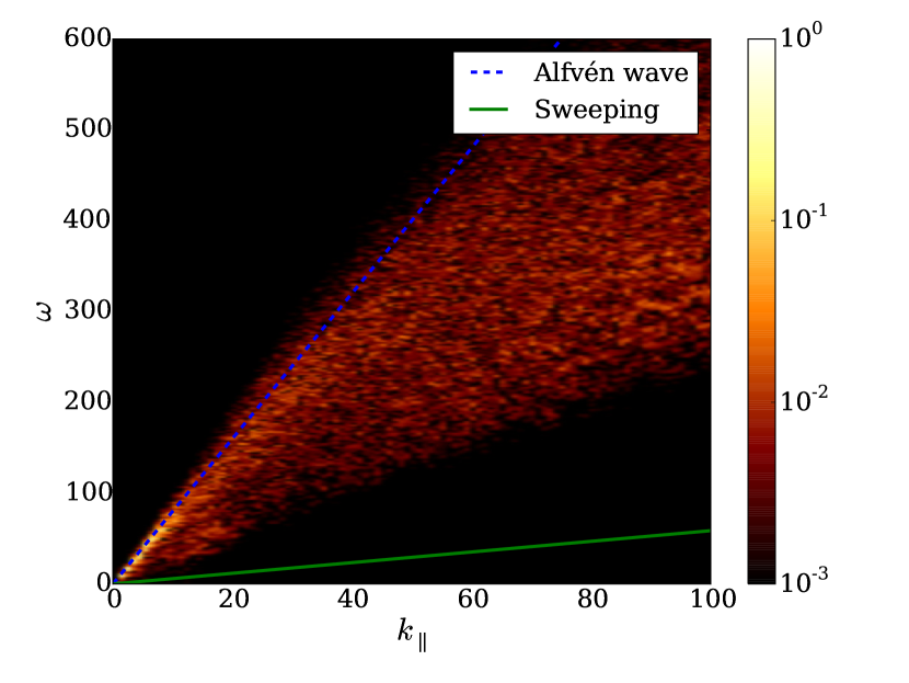
Figure 5: Normalized wave vector and frequency spectrum $E({\bf k},\omega)/E({\bf k})$ for the run with $B_{0}=8$, for modes with $k_{\perp}=0$, and thus as a function of $k_{\parallel}$ and $\omega$. Lighter regions indicate larger energy density. The dashed (blue) line indicates the dispersion relation for Alfvén waves and the continuous (green) line indicates the sweeping relation. Note in this case power is concentrated in a narrow region near the wave dispersion relation up to $k_{\parallel}\approx 10$, corresponding to Alfvénic excitations.

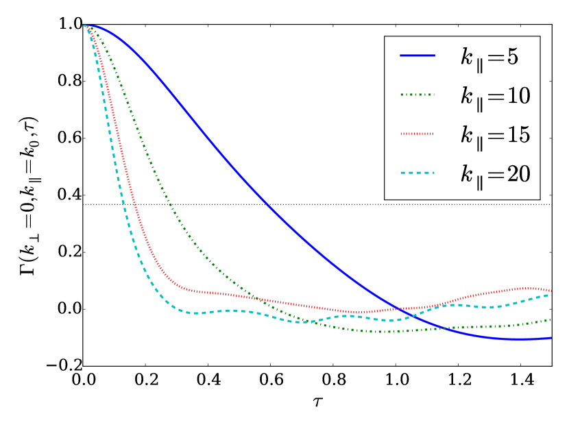
(a) $\Gamma(k_{\perp}=0,k_{\parallel}=k_{0},\tau)$

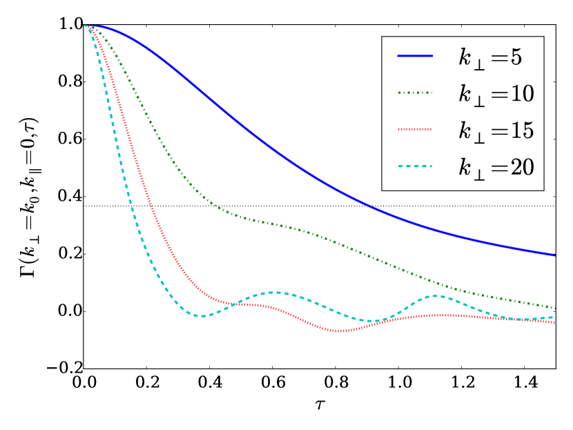
(b) $\Gamma(k_{\perp}=k_{0},k_{\parallel}=0,\tau)$

Figure 6: Correlation functions $\Gamma(k_{\perp}=0,k_{\parallel}=k_{0},\tau)$ and $\Gamma(k_{\perp}=k_{0},k_{\parallel}=0,\tau)$ as a function of the lag time $\tau$, for $k_{0}=5$, 10, 15, and 20, in the simulation with $B_{0}=1$. The value of $\tau$ for which $\Gamma=1/e$ (horizontal dotted line) corresponds to the decorrelation time $\tau_{D}$ for each value of $\mathbf{k}$.

III.3 Correlation functions and decorrelation times

In order to discern between the different phenomena (and relevant time scales) acting in magnetohydrodynamic turbulence, we studied the correlation functions $\Gamma(\mathbf{k},\tau)$ as explained in detail before in Sec. II.2. Since we focus on turbulence with a guide magnetic field, we use $\Gamma(k_{\perp},k_{\parallel},\tau)$ and consider several values of $(k_{\perp},k_{\parallel})$ to study the decorrelation as a function of the time lag $\tau$ at different scales. In Fig. 6, the correlation functions $\Gamma(k_{\perp}=0,k_{\parallel}=k_{0},\tau)$ and $\Gamma(k_{\perp}=k_{0},k_{\parallel}=0,\tau)$ are shown for different values of $k_{0}$ for the moderate external magnetic field $B_{0}=1$. Here we can see the typical behavior of correlation functions, with the largest scales (smallest $k$) taking longer time to decorrelate. Similar results were found for the other external magnetic field considered, $B_{0}=0$, $0.25$, $4$, and $8$.

To understand which of the different times (non-linear time, random sweeping, and Alfvén propagation) are controlling the temporal decorrelation, we need to compare the scaling of the decorrelation time with the theoretical scale dependence expected for each physical process. In order to do this, we use the fact that the mode with wave vector $\mathbf{k}$ should be decorrelated after a time $\tau_{D}(\mathbf{k})$ following an approximate exponential decay

$$\Gamma(\mathbf{k},\tau)\sim e^{-\tau/\tau_{D}(\mathbf{k})}.$$ (10)

For simplicity, we will evaluate $\tau_{D}(\mathbf{k})$ as the time at which the function $\Gamma$ decays to $1/e$ of its initial value.

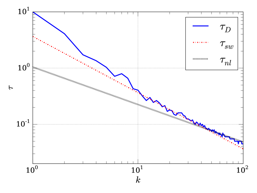
Figure 7: Decorrelation times as a function of $k=|\mathbf{k}|$ for the isotropic case $B_{0}=0$. The straight lines indicate the theoretical predictions corresponding to the sweeping time and the nonlinear time. Except at the largest wavenumbers, the decorrelation time seems to be dominated by sweeping.

As a first example, Fig. 7 shows the decorrelation time $\tau_{D}$ obtained from $\Gamma(k,\tau)$ in the isotropic case with $B_{0}=0$. We can see that the decorrelation time scales in good agreement with the sweeping time, except perhaps at the largest wavenumbers (smallest scales). These results are consistent with the ones obtained by Servidio et al servidio_time_2011 in the isotropic case.

As mentioned before, in the general case it can be difficult to differentiate between the effects of sweeping and Alfvén propagation, as both timescales vary as $k^{-1}$. However, in the anisotropic case (i.e., in the presence of the guide field) we can use the scaling observed with respect to parallel and perpendicular wavenumbers to make the distinction possible. In Fig. 8 we employ results from the $B_{0}=0.25$ run to compute decorrelation times for Fourier modes as a function of $k_{\parallel}$, for several fixed values of $k_{\perp}$. Already for this relatively small value of $B_{0}$ it can be seen that the observed correlation times are closer to the theoretically expected sweeping time than to all the other times (local nonlinear time or Alfvénic time). This is consistent with the results of the wavenumber and frequency energy spectrum shown previously in Fig. 3. A complementary view of the same run with $B_{0}=0.25$ is given in Fig. 9, which shows the decorrelation time $\tau$ as a function of $k_{\perp}$ for several fixed values of $k_{\parallel}$. The conclusion is once again that the sweeping time is controlling $\tau_{D}$ at all but the largest scales, as only for $k_{\perp}=0$ and for $k_{\parallel}$ between $\approx 1$ and $\approx 4$ $\tau_{D}$ is closer to the Alfvén time.

The tendency for time decorrelation to be controlled by sweeping is again seen in the run with the somewhat stronger mean field $B_{0}=1$. These results for the correlation time are shown in in Figs. 10 and 11. Again, only at low values of $k_{\parallel}$ and for $k_{\perp}=0$ it can be seen that the decorrelation time is closer to the Alfvénic time. This tendency was also observed in the wavenumber and frequency spectrum of Fig. 4.

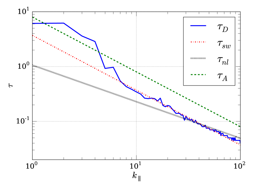
(a) $k_{\perp}=0$

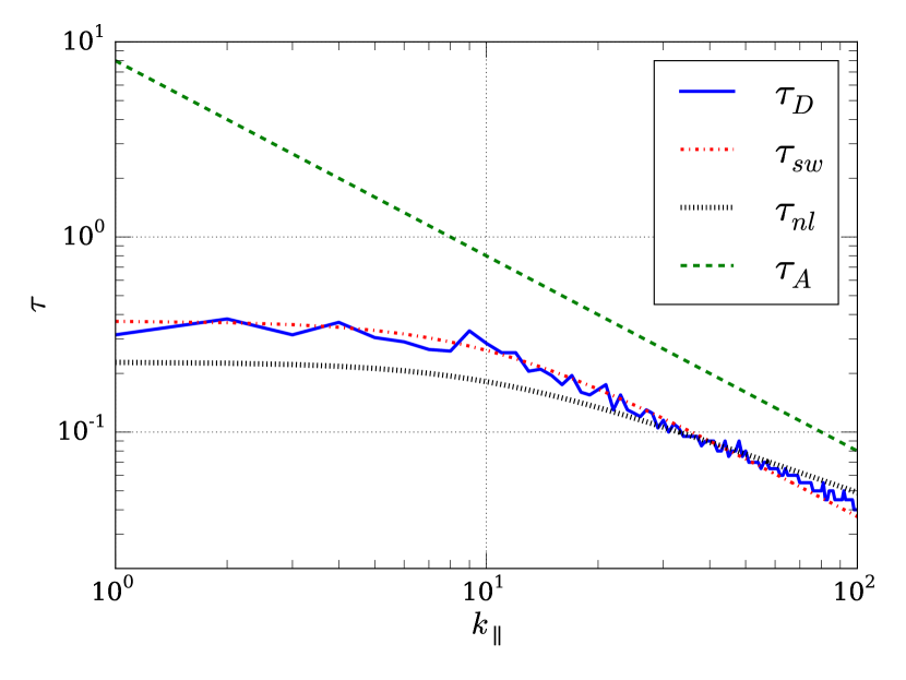
(b) $k_{\perp}=10$

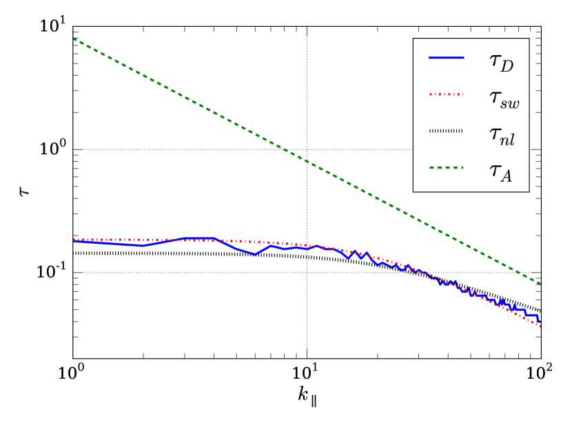
(c) $k_{\perp}=20$

Figure 8: Decorrelation times $\tau_{D}$ for the run with $B_{0}=0.25$. In each panel $k_{\perp}$ is held constant and $k_{\parallel}$ is varied; (a) $k_{\perp}=0$, (b) $k_{\perp}=10$, and (c) $k_{\perp}=20$. The lines indicate theoretical predictions for the scaling of several physical time scales. The measured value of $\tau_{D}$ is always close to $\tau_{sw}$, except for $k_{\perp}=0$ and $k_{\parallel}$ between $\approx 1$ and 5 for which the dominant time scale is the Alfvén time.

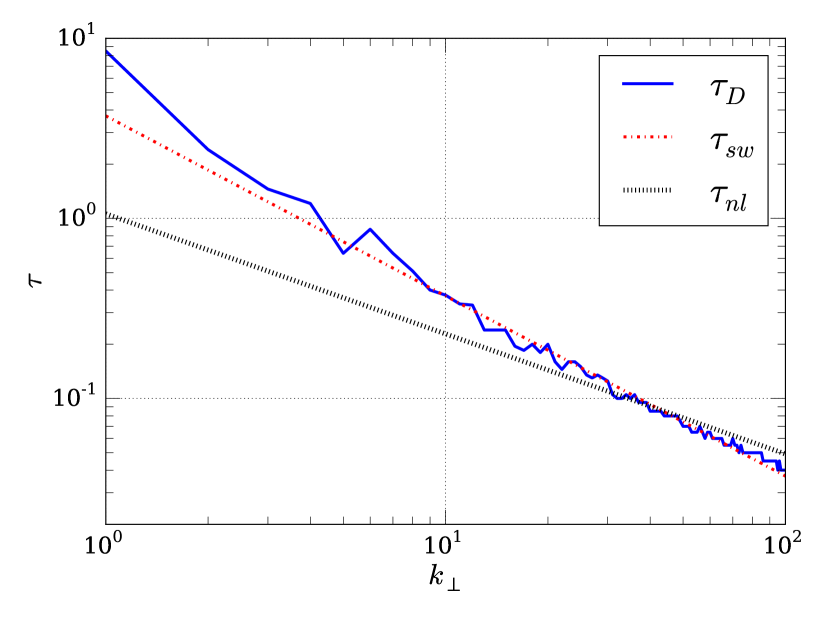
(a) $k_{\parallel}=0$

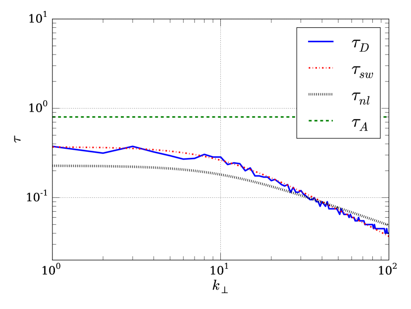
(b) $k_{\parallel}=10$

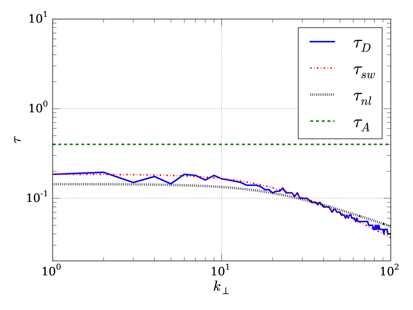
(c) $k_{\parallel}=20$

Figure 9: Decorrelation times $\tau_{D}$ for the run with $B_{0}=0.25$. In each panel $k_{\parallel}$ is held constant and $k_{\perp}$ is varied; (a) $k_{\parallel}=0$, (b) $k_{\parallel}=10$, and (c) $k_{\parallel}=20$. The straight lines indicate theoretical predictions for the scaling of the relevant physical time scales. The measured value of $\tau_{D}$ is always close to $\tau_{sw}$.

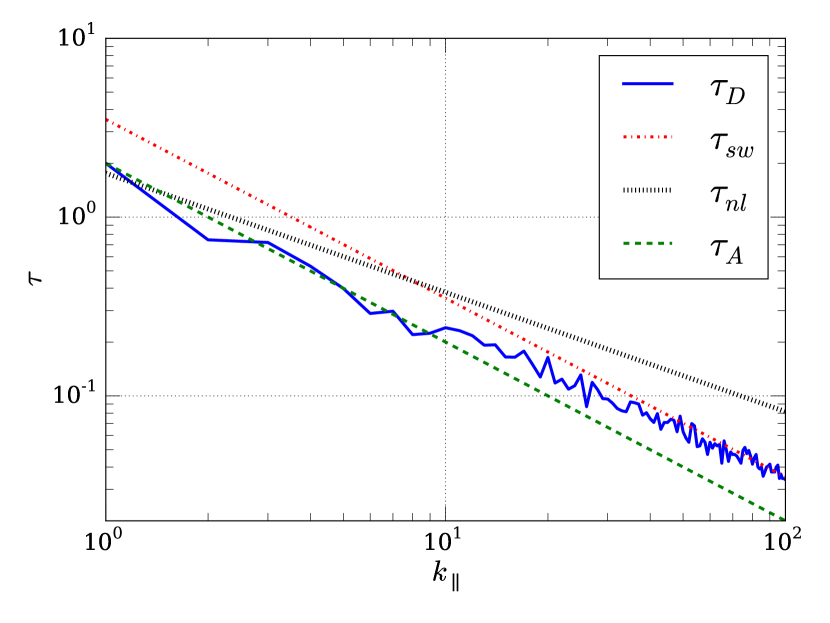
(a) $k_{\perp}=0$

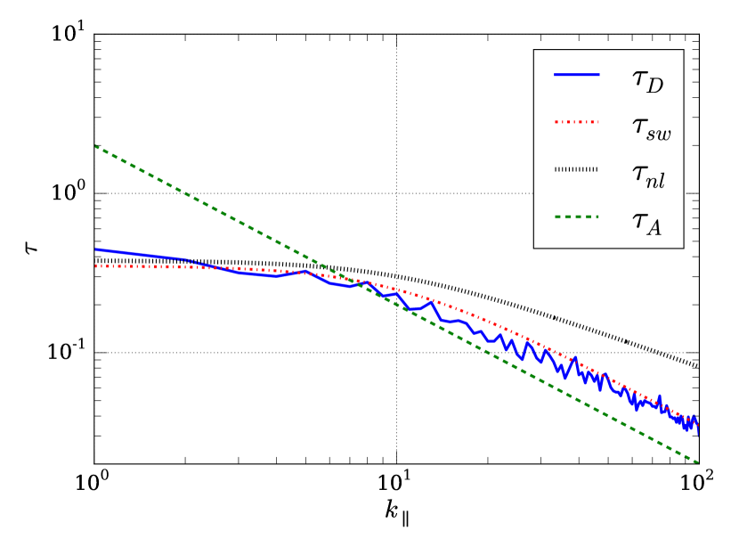
(b) $k_{\perp}=10$

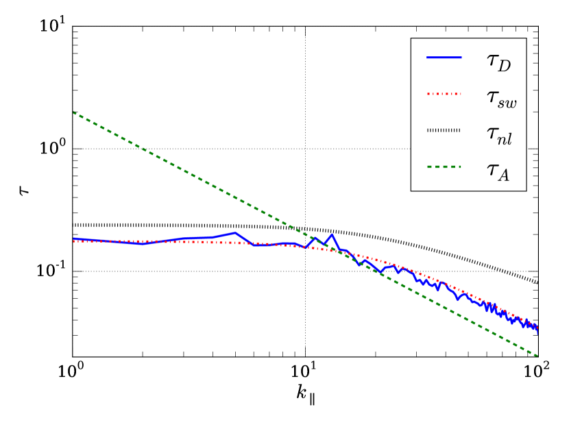
(c) $k_{\perp}=20$

Figure 10: Decorrelation times $\tau_{D}$ for the run with $B_{0}=1$. In each panel $k_{\perp}$ is held constant and $k_{\parallel}$ is varied; (a) $k_{\perp}=0$, (b) $k_{\perp}=10$, and (c) $k_{\perp}=20$. The straight lines indicate theoretical predictions for the scaling of the relevant physical time scales.

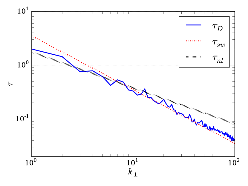
(a) $k_{\parallel}=0$

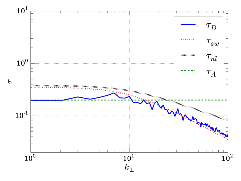
(b) $k_{\parallel}=10$

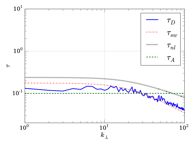
(c) $k_{\parallel}=20$

Figure 11: Decorrelation times $\tau_{D}$ for the run with $B_{0}=1$. In each panel $k_{\parallel}$ is held constant and $k_{\perp}$ is varied; (a) $k_{\parallel}=0$, (b) $k_{\parallel}=10$, and (c) $k_{\parallel}=20$. The straight lines indicate theoretical predictions for the scaling of the relevant physical time scales.

Finally, we analyze the behavior of the decorrelation time $\tau$ for the run with the largest mean magnetic field value that we considered, $B_{0}=8$. The results are presented in Figs. 12 and 13, analyzed in the same way as in the previous two cases. For low values of $k_{\perp}$ one finds that the Alfvénic time dominates the decorrelations (approximately up to $k_{\parallel}=10$, see Fig. 13). For larger values of $k_{\perp}$, however, the decorrelation time departs from the Alfvén time and slowly approaches the sweeping time scale. This is consistent with the spatio-temporal spectrum in Fig. 5, which concentrated energy near the Alfvén dispersion relation for small wavenumbers, but broadened towards the sweeping frequencies for large wave numbers. As a result, it is the competition between these two time scales that for large values of $B_{0}$ seems to be responsible for the broadening of the spatio-temporal spectrum. As long as the Alfvén time is much faster than other time scales in the system, the flow excites Alfvén waves which dominate the mode decorrelation. But as other time scales approach the time scale of the waves (or become faster, as it happens for smaller values of $B_{0}$), the system switches the dominant time scale in the decorrelation.

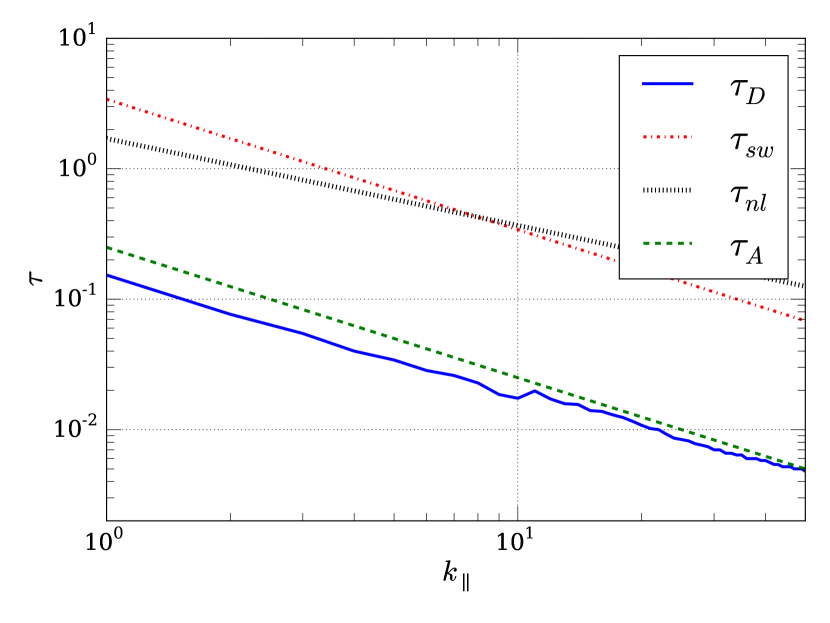
(a) $k_{\perp}=0$

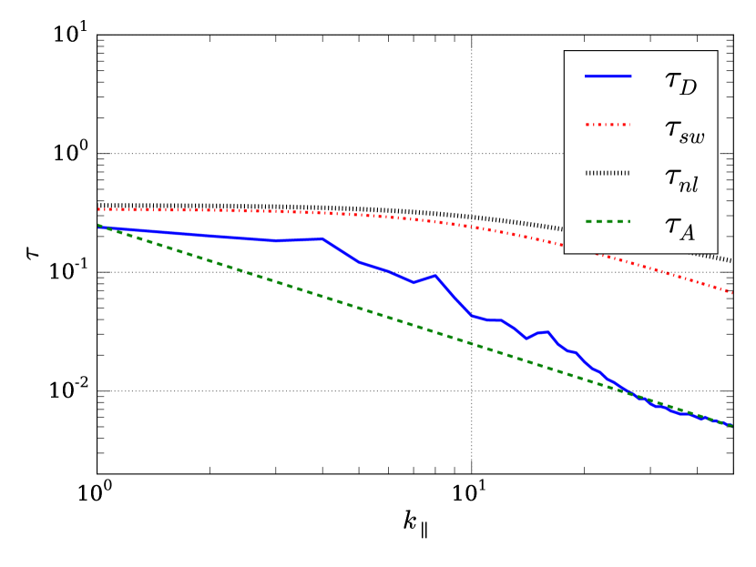
(b) $k_{\perp}=10$

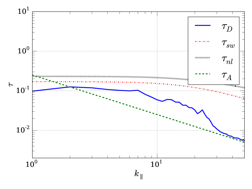
(c) $k_{\perp}=20$

Figure 12: Decorrelation times $\tau_{D}$ for the run with $B_{0}=8$. In each panel $k_{\perp}$ is held constant and $k_{\parallel}$ is varied; (a) $k_{\perp}=0$, (b) $k_{\perp}=10$, and (c) $k_{\perp}=20$. The straight lines indicate theoretical predictions for the scaling of the relevant physical time scales. In this case the Alfvén time controls the decorrelation at multiple wavenumbers.

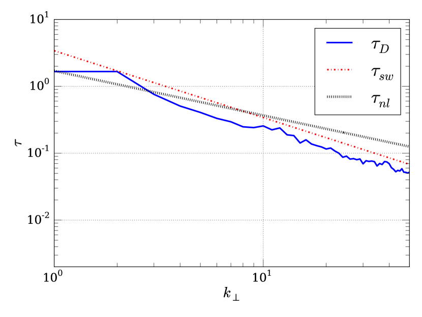
(a) $k_{\parallel}=0$

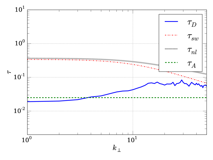
(b) $k_{\parallel}=10$

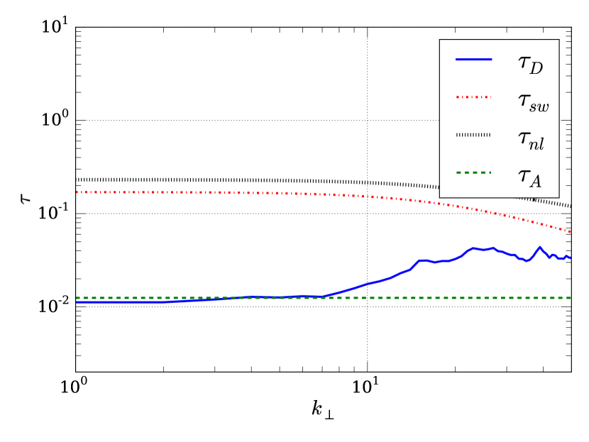
(c) $k_{\parallel}=20$

Figure 13: Decorrelation times $\tau_{D}$ for the run with $B_{0}=8$. In each panel $k_{\parallel}$ is held constant and $k_{\perp}$ is varied; (a) $k_{\parallel}=0$, (b) $k_{\parallel}=10$, and (c) $k_{\parallel}=20$. The straight lines indicate theoretical predictions for the scaling of the relevant physical time scales. The Alfvén time controls the decorrelation up to $k_{\parallel}\approx 10$.

IV Conclusions

In this paper we have studied the time correlations that enter into magnetohydrodynamics in the incompressible approximation. Even in the simpler case of hydrodynamics one expects both space and time correlations to be relevant to the physics of turbulence, as these independent properties can be embodied in the two point, two time correlation $R_{ij}({\bf r},t)$ tensor, e.g., a straightforward generalization of Eq. (3). Analogous correlations may also be written for the components of vector fluid velocity ${\bf u}$ and other quantities. The spatial transform of the correlation (or, equivalently the second order spatial structure functions) at zero time lag $\tau$ provides information about the spatial distribution of energy over scales. Accordingly the zero spatial lag correlation, evaluated at varying time and transformed to frequency, provides analogous information about the distribution of energy over time scales. Here we studied the correlations in time for a given wavenumber or spatial scale for the magnetohydrodynamics model.

The MHD case is more complex than hydrodynamics because two basic fields are involved – velocity and magnetic field. Also because a mean magnetic field is not removed by a Galilean transform, while a mean velocity can be removed in this way. The mean magnetic field therefore imposes a preferred direction. In addition, MHD possesses a new and anisotropic wave mode, the Alfvén mode, that introduces the possibility of spectral and correlation anisotropy, as well as a new times scale, the Alfvén time. Because of these effects the analysis of time decorrelation also become more complex, with at least three time scales to examine – Alfvén, sweeping and nonlinear scales – as well as potential for anisotropy of the decorrelation rate.

Both random sweeping and Alfvénic correlation are non-local effects, in the sense that they couple the large scales with relatively smaller length scales. The results shown here support the conclusion that non-local effects (in spectral space) play an important role in MHD turbulence (in agreement with studies considering shell-to-shell transfers alexakis_turbulent_2007 ; alexakis_anisotropic_2007 ; teaca_energy_2009 ; mininni_scale_2011 ), and that decorrelations are mainly dominated by the sweeping and Alfvénic interactions, confirming previous studies of isotropic MHD servidio_time_2011 . However, compared with the previous studies, the analysis presented here can further distinguish between sweeping and Alfvénic effects, and the results support the conclusion that the sweeping interaction dominates the decorrelation for moderate values of $B_{0}$, while for large values of the mean field $B_{0}$ and at large scales (low perpendicular wavenumbers) the decorrelations are more controlled by the Alfvénic interactions. The relevant interactions are the Alfvén waves, and as such it can be concluded that waves are still present in MHD turbulence and dominate the decorrelations essentially for parallel wavenumbers (aligned with the mean field, see also meyrand_direct_2016 ; meyrand_weak_2015 ). Our results further indicate that the system selects, in effect, the shortest decorrelation time available. A simple and relevant construct is that the rate of decorrelation is the sum of the rates associated with each relevant time scale (see, e.g., zhou_magnetohydrodynamic_2004 ). As a result, even for large values of the guide field $B_{0}$, for sufficiently small scales in which the sweeping time becomes faster than the Alfvénic time, after a broad range of scales dominated by Alfvén waves the system transitions to a sweeping dominated behaviour.

It is of interest to recall that the relevant time decorrelation associated with energy transfer in turbulence is not the Eulerian time correlation that we have considered (fixed spatial point, varying time), but rather the Lagrangian time decorrelation, computed following a material fluid element. In this regard, it is well known that neither sweeping nor Alfvénic wave propagation can directly produce spectral transfer in idealized homogeneous models. In part due to these complications, no complete theory exists at present that links the spatial correlation and the time correlations in MHD or hydrodynamic turbulence. On the other hand it is clear that in MHD, both sweeping and Alfvén wave propagation contribute to the total time variation at a point (Eulerian frequency spectrum), and are therefore influential in limiting prediction. These time scales are also important features in understanding the scattering of charged test particles, such as low energy cosmic rays bieber_proton_1994 , as well as in accounting for the distribution of accelerations, which is related to intermittency nelkin_time_1990 .

The observed behavior of MHD time decorrelation, exemplified by the new results presented here, thus have applications in a number of subjects, including charged particle scattering theory schlickeiser_cosmic-ray_1993 ; nelkin_time_1990 , interplanetary magnetic field and magnetospheric dynamic miller_critical_1997 , and interpretation of spacecraft data from historical and future missions matthaeus_ensemble_2016 . Looking towards future prospects, we note that there has been some success in establishing empirical connections between the sweeping time scale to the observed Eulerian time decorrelation in hydrodynamics chen_sweeping_1989 . Similar ideas for MHD (e.g., matthaeus_dynamical_1999 ) might be exploited to better understand, or at least empirically model, the relationship in MHD between spatial structure and time decorrelation, an effort that would directly benefit from the novel results presented here.

V Acknowledgments

R.L., P.D., and P.D.M. acknowledge support from the grants UBACyT No. 20020110200359 and 20020100100315, and PICT No. 2011-1529, 2011-1626, and 2011-0454.

W.H.M. is partially supported by NASA LWS-TRT grant NNX15AB88G, NASA Grant NNX14AI63G (Heliophysics Grand Challenge Theory), and the Solar Probe Plus mission through the Southwest Research Institute ISOIS project D99031L.

References

- (1) P. Dmitruk and W. H. Matthaeus. Waves and turbulence in magnetohydrodynamic direct numerical simulations. Physics of Plasmas (1994-present), 16(6):062304, June 2009.
- (2) A. S. Monin and A. M. Yaglom. Statistical Fluid Mechanics, Volume II: Mechanics of Turbulence. Courier Corporation, July 2013.
- (3) A. N. Kolmogorov. The Local Structure of Turbulence in Incompressible Viscous Fluid for Very Large Reynolds Numbers. C. R. Acad. Sci. URSS, 30(4):301–305, 1941.
- (4) W. D. McComb. The Physics of Fluid Turbulence. Clarendon Press, February 1992.
- (5) A. Alexakis, P. D. Mininni, and A. Pouquet. Turbulent cascades, transfer, and scale interactions in magnetohydrodynamics. New J. Phys., 9(8):298, 2007.
- (6) A. Alexakis, B. Bigot, H. Politano, and S. Galtier. Anisotropic fluxes and nonlocal interactions in magnetohydrodynamic turbulence. Phys. Rev. E, 76(5):056313, November 2007.
- (7) B. Teaca, M. K. Verma, B. Knaepen, and D. Carati. Energy transfer in anisotropic magnetohydrodynamic turbulence. Phys. Rev. E, 79(4):046312, April 2009.
- (8) P. D. Mininni. Scale Interactions in Magnetohydrodynamic Turbulence. Annual Review of Fluid Mechanics, 43(1):377–397, 2011.
- (9) R. H. Kraichnan. The structure of isotropic turbulence at very high Reynolds numbers. Journal of Fluid Mechanics, 5(04):497–543, May 1959.
- (10) H. Tennekes. Eulerian and Lagrangian time microscales in isotropic turbulence. Journal of Fluid Mechanics, 67(03):561–567, February 1975.
- (11) S. Chen and R. Kraichnan. Sweeping decorrelation in isotropic turbulence. Physics of Fluids A: Fluid Dynamics (1989-1993), 1(12):2019–2024, December 1989.
- (12) M. Nelkin and M. Tabor. Time correlations and random sweeping in isotropic turbulence. Physics of Fluids A: Fluid Dynamics (1989-1993), 2(1):81–83, January 1990.
- (13) A. Pouquet, U. Frisch, and J. Léorat. Strong MHD helical turbulence and the nonlinear dynamo effect. Journal of Fluid Mechanics, 77(02):321–354, September 1976.
- (14) Y. Zhou, W. H. Matthaeus, and P. Dmitruk. Magnetohydrodynamic turbulence and time scales in astrophysical and space plasmas. Rev. Mod. Phys., 76(4):1015–1035, December 2004.
- (15) S. A. Orszag and G. S. Patterson. Numerical Simulation of Three-Dimensional Homogeneous Isotropic Turbulence. Phys. Rev. Lett., 28(2):76–79, January 1972.
- (16) S. A. Orszag. Analytical theories of turbulence. Journal of Fluid Mechanics, 41(02):363–386, April 1970.
- (17) W. Heisenberg. Zur statistischen Theorie der Turbulenz. Z. Physik, 124(7-12):628–657, July 1948.
- (18) G. Comte-Bellot and S. Corrsin. Simple Eulerian time correlation of full-and narrow-band velocity signals in grid-generated, turbulence. Journal of Fluid Mechanics, 48(02):273–337, July 1971.
- (19) Y. Zhou, A. A. Praskovsky, and G. Vahala. A non-Gaussian phenomenological model for higher-order spectra in turbulence. Physics Letters A, 178(1):138–142, July 1993.
- (20) T. Sanada and V. Shanmugasundaram. Random sweeping effect in isotropic numerical turbulence. Physics of Fluids A: Fluid Dynamics (1989-1993), 4(6):1245–1250, June 1992.
- (21) S. Servidio, V. Carbone, P. Dmitruk, and W. H. Matthaeus. Time decorrelation in isotropic magnetohydrodynamic turbulence. EPL, 96(5):55003, 2011.
- (22) W. H. Matthaeus, S. Dasso, J. M. Weygand, M. G. Kivelson, and K. T. Osman. Eulerian Decorrelation of Fluctuations in the Interplanetary Magnetic Field. ApJ, 721(1):L10, 2010.
- (23) F. Carbone, L. Sorriso-Valvo, C. Versace, G. Strangi, and R. Bartolino. Anisotropy of Spatiotemporal Decorrelation in Electrohydrodynamic Turbulence. Phys. Rev. Lett., 106(11):114502, March 2011.
- (24) P. Clark di Leoni, P. J. Cobelli, P. D. Mininni, P. Dmitruk, and W. H. Matthaeus. Quantification of the strength of inertial waves in a rotating turbulent flow. Physics of Fluids (1994-present), 26(3):035106, March 2014.
- (25) P. Clark di Leoni, P. J. Cobelli, and P. D. Mininni. The spatio-temporal spectrum of turbulent flows. Eur. Phys. J. E, 38(12):136, December 2015.
- (26) R. Meyrand, S. Galtier, and K. H. Kiyani. Direct Evidence of the Transition from Weak to Strong Magnetohydrodynamic Turbulence. Phys. Rev. Lett., 116(10):105002, March 2016.
- (27) R. Meyrand, K. H. Kiyani, and S. Galtier. Weak magnetohydrodynamic turbulence and intermittency. Journal of Fluid Mechanics, 770:R1 (11 pages), May 2015.
- (28) D. O. Gómez, P. D. Mininni, and P. Dmitruk. Parallel Simulations in Turbulent MHD. Phys. Scr., 2005(T116):123, 2005.
- (29) D. O. Gómez, P. D. Mininni, and P. Dmitruk. MHD simulations and astrophysical applications. Advances in Space Research, 35(5):899–907, 2005.
- (30) P. D. Mininni, D. Rosenberg, and A. Pouquet. Isotropization at small scales of rotating helically driven turbulence. Journal of Fluid Mechanics, 699:263–279, May 2012.
- (31) J. W. Bieber, W. H. Matthaeus, C. W. Smith, W. Wanner, MB Kallenrode, and G. Wibberenz. Proton and electron mean free paths: The Palmer consensus revisited. The Astrophysical Journal, 420:294–306, January 1994.
- (32) R. Schlickeiser and U. Achatz. Cosmic-ray particle transport in weakly turbulent plasmas. Part 1. Theory. Journal of Plasma Physics, 49(01):63–77, February 1993.
- (33) J. A. Miller, P. J. Cargill, A. G. Emslie, G. D. Holman, B. R. Dennis, T. N. LaRosa, R. M. Winglee, S. G. Benka, and S. Tsuneta. Critical issues for understanding particle acceleration in impulsive solar flares. J. Geophys. Res., 102(A7):14631–14659, January 1997.
- (34) W. H. Matthaeus, J. M. Weygand, and S. Dasso. Ensemble Space-Time Correlation of Plasma Turbulence in the Solar Wind. Phys. Rev. Lett., 116(24):245101, June 2016.
- (35) W. H. Matthaeus and J. W. Bieber. Dynamical scattering theory and observations of particle diffusion in the heliosphere. In AIP Conference Proceedings, volume 471, pages 515–518. AIP Publishing, June 1999.