Clustering determines the dynamics of complex contagions in multiplex networks

Abstract

We present the mathematical analysis of generalized complex contagions in clustered multiplex networks for susceptible-infected-recovered (SIR)-like dynamics. The model is intended to understand diffusion of influence, or any other spreading process implying a threshold dynamics, in setups of interconnected networks with significant clustering. The contagion is assumed to be general enough to account for a content-dependent linear threshold model, where each link type has a different weight (for spreading influence) that may depend on the content (e.g., product, rumor, political view) that is being spread. Using the generating functions formalism, we determine the conditions, probability, and expected size of the emergent global cascades. This analysis provides a generalization of previous approaches and is specially useful in problems related to spreading and percolation. The results present non trivial dependencies between the clustering coefficient of the networks and its average degree. In particular, several phase transitions are shown to occur depending on these descriptors. Generally speaking, our findings reveal that increasing clustering decreases the probability of having global cascades and their size, however this tendency changes with the average degree. There exists a certain average degree from which on clustering favours the probability and size of the contagion. By comparing the dynamics of complex contagions over multiplex networks and their monoplex projections, we demonstrate that ignoring link types and aggregating network layers may lead to inaccurate conclusions about contagion dynamics, particularly when the correlation of degrees between layers is high.

PACS numbers

I Introduction

The study of dynamical processes on real-world complex networks has been an active research area over the past decade. Some of the most widely studied problems include cascading failures in interdependent networks Buldyrev et al. (2010); Vespignani (2010); Yağan et al. (2012); Brummitt et al. (2012a); Radicchi and Arenas (2013); Reis et al. (2014), simple contagions (e.g., diffusion of information, disease propagation in human and animal populations Albert et al. (2000); Cohen et al. (2000, 2002); Leicht and D’Souza (2009); Nagler et al. (2011); Murray (2002); Son et al. (2011); Baxter et al. (2012); Dickison et al. (2012); Anderson and May (1991); Sahneh et al. (2013); Yağan et al. (2013); Valdez et al. (2013); Zhao and Bianconi (2013); Cellai et al. (2013); Azimi-Tafreshi et al. (2014); Bianconi and Dorogovtsev (2014); Radicchi (2015), etc.), and complex contagions (e.g., diffusion of influence, beliefs, norms, and innovations in social networks Gleeson (2008); Watts (2002); Yağan and Gligor (2012)). Recently, the attention was shifted from single, isolated networks to multiplex and multi-layer networks Hackett et al. (2016); Sahneh et al. (2013); Yağan et al. (2013); Yağan and Gligor (2012); Zhuang and Yağan (2016); Brummitt et al. (2012b); Kivelä et al. (2014); De Domenico et al. (2014, 2013); Min et al. (2014); Serrano et al. (2015); Granell et al. (2013); Baxter et al. (2014); De Domenico et al. (2016); Wu et al. (2016); Boccaletti et al. (2014); Cellai and Bianconi (2016). This shift is primarily driven by the observation that links in a network might be categorized according to the nature of the relationship they represent (e.g., friends, family, office-mates) as well as according to the social network they belong (e.g., Google+ vs. Facebook links), and each link type might play a different role in the dynamical process.

In this work, we focus on the analysis of complex contagion processes that take place on multiplex (or, multi-layer) networks. In doing so, we adopt the content-dependent linear threshold model of social contagions proposed by Yağan and Gligor Yağan and Gligor (2012). Their framework is a generalization of the linear threshold model introduced by Watts Watts (2002) and is based on individuals adopting a behavior when their perceived proportion of active neighbors exceed a certain threshold; the key to that modeling framework is that one’s perceived influence depends on the types of the relationships they have and the context in which diffusion is being considered. More precisely, each individual in the network can be in one of the two states, active or inactive. Each link type-$i$ is associated with a content-dependent weight $c_{i}$ in $[0,\infty]$ that encodes the relative importance of this link type in spreading the given content. Then, an inactive node with $m_{i}$ active neighbors and $d_{i}-m_{i}$ inactive neighbors via type-$i$ links turns active only if

$$\frac{\sum_{i}c_{i}m_{i}}{\sum_{i}c_{i}d_{i}}\geq\tau$$

where $\tau$ is the node’s threshold drawn from a distribution $P(\tau)$. Once active, a node stays active forever.

Yağan and Gligor analyzed Yağan and Gligor (2012) the content-dependent linear threshold model in multiplex networks and derived the conditions, probability, and expected size of global cascades, i.e., cases where activating a randomly selected node leads to activation of a positive fraction of the population in the limit of large system sizes. However, their multiplex network model was formed by combining independent layers of networks (one for each link type), where each layer is generated by the configuration model Newman et al. (2001); Newman (2003). Although a good starting point, configuration model is known to generate networks that can not accurately capture some important aspects of real-world social networks, most notably the property of high clustering Watts and Strogatz (1998); Serrano and Boguñá (2006). Informally known as the phenomenon that “friends of our friends” are likely to be our friends, clustering has been shown to affect the dynamics of various diffusion processes Newman (2009); Gleeson et al. (2010); Hackett et al. (2011a, b); Huang et al. (2013); Colomer-de Simón and Boguñá (2014); Zhuang and Yağan (2016); Cozzo et al. (2015) significantly.

With this in mind, our main contribution in this paper is to provide a thorough analysis of influence diffusion process (a complex contagion) in clustered multiplex networks. In particular, we study the content dependent linear threshold model in a multiplex network model where each link type (or, network layer) is formed by the clustered random network model proposed by Newman Newman (2009) and Miller Miller (2009). We solve for the critical threshold, probability, and expected size of global cascades and confirm our analytical results via extensive simulations. The main observation from our results is that clustering has a double-faceted impact on the probability and expected size of global cascades. Namely, we show that clustering decreases the probability and size of cascades when average degree in the network is small, whereas after a certain value of average degree, clustering is shown to facilitate cascades.

We also compare the dynamics of complex contagions over multiplex networks and their monoplex projections. There has been recent interest Hackett et al. (2016) in understanding whether monoplex projection of a multiplex network (obtained by ignoring the colors of edges and aggregating the layers) can still capture the essential properties (e.g., cascade threshold and size) of a diffusion process. In the affirmative, this would eliminate the need for considering the full multiplex structure of real-world systems in tackling similar problems. We show that even in the simplest case where all link types have the same influence weight (i.e., $c_{1}=c_{2}=\cdots$), monoplex theory may not be able to capture contagion dynamics accurately, reinforcing the need for studying multiplex networks in its correct setup. We demonstrate that the accuracy of monoplex theory in capturing cascade dynamics over multiplex networks depends tightly on the assortativity (i.e., correlation between the degrees of connected pairs) of the network. For instance, when assortativity is negligible, monoplex theory is seen to predict cascade dynamics very well, while in highly assortative cases its ability to predict contagion behavior diminishes significantly.

Finally, we proof the possibility of an unforeseen behavior in the dynamics of complex contagions in multiplex networks, i.e., that of observing more than two phase transitions in the cascade size as the mean degrees in network layers increase. It has been reported Watts (2002); Yağan et al. (2013) many times that threshold models of complex contagion exhibit two phase transitions as the average degree increases; a second-order transition at low degrees marking the formation of a giant component of vulnerable nodes and a first-order transition at high degrees due to increased local stability of nodes. Here, we consider a multiplex where one layer has degree distribution $\textrm{Poi}(\lambda)$ while the degree in the second layer follows $\textrm{Poi}(\lambda/\alpha)$ with probability $\alpha$ and is zero with probability $1-\alpha$. In this setting, we observe that in general there exist two intervals of $\lambda$ for which cascades are possible, amounting to four phase transitions as opposed to two; also, it is seen that only the first transition is second-order while the remaining ones are first order. However, depending on the value of $\alpha$, these regions may overlap (with overlap starting when $\alpha$ exceeds a critical value) resulting again with only two phase transitions; see Section VI.3 for details.

The paper is organized as follows. We give details of the models applied in this study and the problem to be considered in Section II. In Sections III and IV we present the main results of this work, and confirm it through extensive computer simulations in Section V. In Section VI, we make a comparison between complex contagions in monoplex networks and multiplex networks, and also demonstrate the new phenomenon about the number of phase transitions. Finally, Section VII summarizes our work and gives future directions.

II Model: structure and dynamics

II.1 Random Graphs with Clustering

Our goal is to study complex contagion processes in synthetic networks that capture some important aspects of real-world networks but otherwise are generated randomly. It is known Newman et al. (2001); Newman (2003) that the widely used configuration model Newman et al. (2001) generates tree-like graphs with number of cycles approaching to zero as the number of nodes gets large. However, most social networks exhibit high clustering, informally known as the propensity of a “friend of a friend” to be one’s friend. Put differently, real-world social networks are usually not tree-like and instead have considerable number of cycles, particularly of size three; i.e., triangles. With this in mind, Miller Molloy and Reed (1995) and Newman Newman (2003) proposed a modification on the configuration model to enable generating random graphs with given degree distributions and tunable clustering.

The model proposed in Molloy and Reed (1995); Newman (2003) is often referred to as random networks with clustering and is based on the following algorithm. Given a joint degree distribution $\{p_{st}\}_{s,t=0}^{\infty}$ that gives the probability that a node has $s$ single edges and $t$ triangles, each node will be given $s$ stubs labeled as single and $2t$ stubs labeled as triangles with probability $p_{st}$, for any $s,t=0,1,\ldots$. Then, stubs that are labeled as single are randomly joined to form single edges that are not part of a triangle, whereas pairs of triangle stubs from three nodes are randomly matched to form triangles between the three participating nodes; the total degree of a node is then distributed by $p_{k}=\sum_{s,t:s+2t=k}p_{st}$. As in the standard configuration model, it can be shown that the number of cycles formed by single edges goes to zero as $n$ gets large, and so does the number of cycles of length larger than three Newman et al. (2001).

We quantify the level of clustering using the widely recognized global clustering coefficient Newman (2003), defined via

$$C_{\textrm{global}}=\frac{3\times(\text{number of triangles in network})}{\text{number of connected triples}}.$$

Here, “connected triples” means a single vertex connected by edges to two others. It was shown in Newman et al. (2001) that $C_{\textrm{global}}$ is positive in the random clustered network model, while it approaches to zero with increasing network size in the standard configuration model.

Figure 1: Illustration of multi-layer and multiplex network representations of our model. In (a), we see a multilayer network (e.g., a Physical communication layer and a Facebook layer) with overlapping vertex sets; vertical dashed lines represent nodes corresponding to the same individual. In (b), we see the equivalent representation of this model by a multiplex network. Edges from Facebook are shown in red and edges from the physical network are shown in blue.

II.2 Multi-layer and Multiplex Network Models

In this paper, we consider a multiplex network where links are classified into different types, or colors. For ease of exposition, we consider the case with only two colors, red and blue, but the discussion can easily be extended to arbitrary number of colors. Let ${\mathbb{R}}$ and ${\mathbb{B}}$ denote the sub-networks formed by red and blue edges, respectively. A possible motivation is that ${\mathbb{R}}$ models the kinship contact network among individuals, while the network ${\mathbb{B}}$ stands for the colleagueship network. Alternatively, we can think of ${\mathbb{B}}$ modeling the physical (e.g., face-to-face) relationships among human beings while ${\mathbb{R}}$ models connections through an online social network (e.g., Facebook).

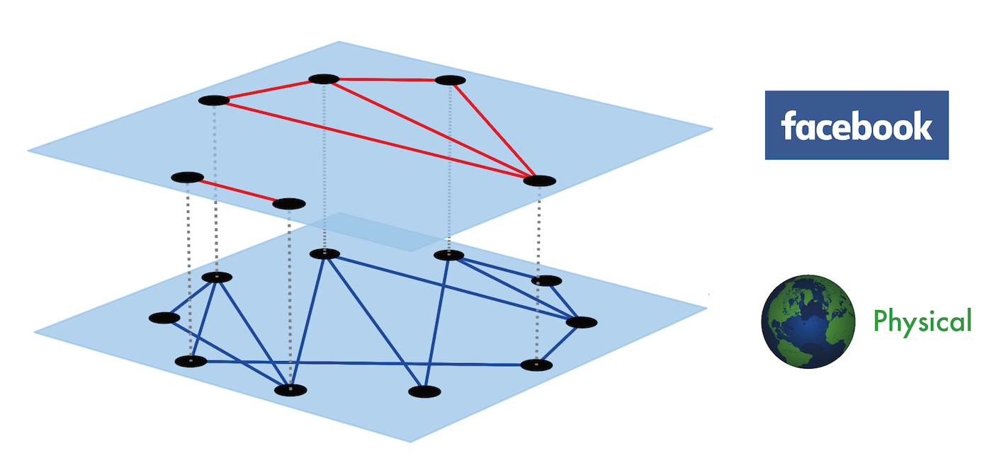
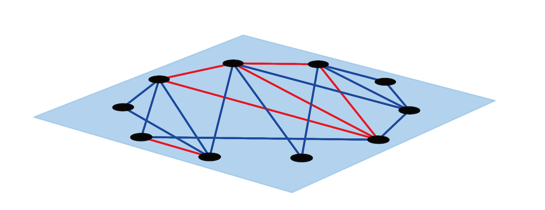
In line with the second motivation, we assume that network ${\mathbb{B}}$ is defined on the vertices $\mathcal{N}=\{1,\dots,n\}$, while ${\mathbb{R}}$ contains only a subset of the nodes in $\mathcal{N}$ to account for the fact that not every individual participates in online social networks; e.g., we assume that each vertex in $\mathcal{N}$ participates in ${\mathbb{R}}$ independently with probability $\alpha\in(0,1]$, meaning that the set of vertices of ${\mathbb{R}}$ constitutes $\alpha$-fraction of the whole population. We illustrate in Figure 1 two equivalent representations of this model, first shown as a multi-layer network with overlapping vertex sets, and second as a multiplex network.

We generate both ${\mathbb{R}}$ and ${\mathbb{B}}$ from the generalized configuration model described in Section II.1; i.e., both are random networks with clustering. In particular, we let $\{p_{st}^{r},s,t=0,1,\dots\}$ and $\{p_{st}^{b},s,t=0,1,\dots\}$ denote the joint distributions for single edges and triangles for ${\mathbb{R}}$ and ${\mathbb{B}}$, respectively. Then both networks are generated independently according to the algorithm described in Section II.1, and they are denoted respectively by ${\mathbb{R}}={\mathbb{R}}(n;\alpha,p_{st}^{r})$ and ${\mathbb{B}}={\mathbb{B}}(n;p_{st}^{b})$. We define the overall network ${\mathbb{H}}$ over which influence spreads as the disjoint union ${\mathbb{H}}={\mathbb{R}}\coprod{\mathbb{B}}$ and represent it by ${\mathbb{H}}(n;\alpha,p_{st}^{r},p_{st}^{b})$. Here, the disjoint union operation implies that we still distinguish ${\mathbb{R}}$-edges from ${\mathbb{B}}$-edges in ${\mathbb{H}}$, meaning that it is a multiplex network.

We denote the colored degree $\mathbf{d}$ of a node in ${\mathbb{H}}$ by

$$\mathbf{d}=(d_{rs},2n_{rt},d_{bs},2n_{bt})$$ (1)

meaning that it has $d_{rs}$ single edges and $2n_{rt}$ triangle edges in network ${\mathbb{R}}$, and $d_{bs}$ single edges and $2n_{bt}$ triangle edges in network ${\mathbb{B}}$; here $n_{rt}$ and $n_{bt}$ are defined as the number of triangles assigned to this node in ${\mathbb{R}}$ and ${\mathbb{B}}$, respectively. The distribution of this colored degree is denoted by $p_{\mathbf{d}}$ and can be computed directly from $p_{st}^{r}$, $p_{st}^{b}$ and $\alpha$.

Figure 2: Illustration of three cases that would be counted as $m_{rs}$, $m_{rt1}$, and $m_{rt2}$, respectively for the number of active nodes. Nodes shown in filled (green) circles are active while those shown in non-filled circles are inactive.

II.3 Content-dependent Linear Threshold Model for Social Contagion

The classical linear threshold model by Watts Watts (2002) is based on indviduals adopting a behavior when the fraction of their active neighbors exceed a certain threshold. Namely, an inactive node $i$ with $m_{i}$ active neighbors and $d_{i}-m_{i}$ inactive neighbors will become active only if $m_{i}/d_{i}$ exceeds $\tau_{i}$ drawn from a distribution $P(\tau)$; once active, a node can not be deactivated. A major concern with this model is that it assumes all links in the network have the same importance, irrespective of the context that the spreading is being considered. However, in real world contagion processes, each link type (e.g., co-workership vs. family or physical links vs. online social network links) may play a different role in different cascade processes. For example, in the spread of a new consumer product amongst the population, a video game would be more likely to be promoted among high school classmates rather than among family members; the situation would be exactly the opposite in the case of a new cleaning product Tang et al. (2011).

To address the aforementioned drawbacks, Yağan and Gligor Yağan and Gligor (2012) proposed a content-dependent linear threshold model for social contagion in multiplex networks. In this model, each link type is associated with a content dependent parameter $c_{i}$ in $[0,\infty]$ that measures the relative bias type-$i$ links have in spreading the content. Then, an inactive node with $m_{i}$ active neighbors and $d_{i}-m_{i}$ inactive neighbors through link type-$i$ will turn active if $\frac{\sum_{i}c_{i}m_{i}}{\sum_{i}c_{i}d_{i}}\geq\tau$.

In this work, we will analyze complex contagions in ${\mathbb{H}}$ under the content-dependent threshold model introduced in Yağan and Gligor (2012). Consider a node with colored degree ${{\mathbf{d}}}=\left(d_{rs},2n_{rt},d_{bs},2n_{bt}\right)$ and active-degree

$${{\mathbf{m}}}=\left(m_{rs},m_{rt1},m_{rt2},m_{bs},m_{bt1},m_{bt2}\right),$$

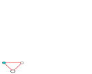
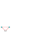
where $m_{rs}$ (resp. $m_{bs}$) gives the number of active neighbors connected through red single edges (resp. blue single edges), and $m_{rt1}$ and $m_{rt2}$ (resp. $m_{bt1}$ and $m_{bt2}$) give the number of red (resp. blue) triangles with one and two active neighbors, respectively; see Figure 2 for demonstration of three cases counted as $m_{rs}$, $m_{rt1}$, and $m_{rt2}$, respectively. Next, for a given content to spread over ${\mathbb{H}}$, let $c_{r}$ and $c_{b}$ denote the weight of $red$- and $blue$-edges, respectively, in spreading this content. Without loss of generality, we set $c:=\frac{c_{r}}{c_{b}}$. Then, the probability that an inactive node with degree ${{\mathbf{d}}}$ and active-degree ${{\mathbf{m}}}$ turns active is given by

$$F({{\mathbf{m}}},{{\mathbf{d}}})$$ (2)

$$={\mathbb{P}}\left[\frac{c\left(m_{rs}+m_{rt1}+2m_{rt2}\right)+m_{bs}+m_{bt1}+2m_{bt2}}{c\left(d_{rs}+2n_{rt}\right)+d_{bs}+2n_{bt}}\geq\tau\right]$$

Hereafter, the function $F({{\mathbf{m}}},{{\mathbf{d}}})$ will be referred to as the neighborhood response function Dodds and Watts (2004); Hackett et al. (2011b).

II.4 The Problem

We consider the diffusion of influence over ${\mathbb{H}}$ that is initiated by a randomly selected node. Our main goal is to derive the conditions, probability, and expected size of global cascades, i.e., cases where influence starts from a single individual and reaches a positive fraction of the population in the large $n$ limit. Of particular interest will be to reveal the effect of clustering coefficient $C_{\textrm{global}}$ and content parameter $c$ on these quantities.

III Condition and Probability of Global Cascades

In this section, we derive the condition and probability of global cascades in clustered multiplex networks; expected size of global cascades is handled separately in Section IV. As mentioned in Section II.2, we restrict our attention to networks with only two link types, labeled as blue and red edges, respectively. Distinguishing further the edges based on whether or not they are part of a triangle, we obtain four types of edges in our clustered multiplex network model, labeled as red single edges, red triangles edges, blue single edges, and blue triangle edges; these are denoted by $rs-$, $rt-$, $bs-$, and $bt-$, respectively.

To analyze the influence diffusion process, we consider a branching process Athreya and Ney (2012) that starts by activating a node selected randomly from among all nodes. Starting with the neighbors of the seed node, we explore and identify all nodes that are reached and activated, continuing recursively until the branching process stops. Let $H(x)$ denote the generating function Wilf (2013) for the “finite number of nodes that are reached and influenced” by the branching process Athreya and Ney (2012) initiated by a randomly selected node. We will derive an expression for $H(x)$ using $h_{rs}(x)$, $h_{rt}(x)$, $h_{bs}(x)$, and $h_{bt}(x)$, where $h_{rs}(x)$ (resp. $h_{bs}(x)$) stands for the generating function for the “finite number of nodes reached by following a randomly selected red single (resp. blue single) edge”; $h_{rt}(x)$ and $h_{bt}(x)$ are defined similarly for red triangle and blue triangle edges, respectively. Then, $H(x)$ takes the form

$$H(x)=x\sum_{{{\mathbf{d}}}}{p_{\mathbf{d}}}D(d_{rs},n_{rt},d_{ws},n_{wt}),$$ (3)

where

$$D(y,z,m,\ell):=h_{rs}(x)^{y}h_{rt}(x)^{z}h_{bs}(x)^{m}h_{bt}(x)^{\ell}$$ (4)

The validity of (3) can be seen as follows. The term $x$ stands for the node that is selected randomly and set active to initiate the cascade. This node has a degree ${{\mathbf{d}}}=\left(d_{rs},2n_{rt},d_{bs},2n_{bt}\right)$ with probability ${p_{\mathbf{d}}}$. The number of nodes reached by each of its $d_{rs}$ (resp. $d_{bs}$) red single edges (resp. blue single edges) has a generating function $h_{rs}(x)$ (resp. $h_{bs}(x)$). Considering its triangle edges in a similar manner, we see from the powers property of generating functions Newman et al. (2001) that when the initial node has degree ${{\mathbf{d}}}$ the number of nodes influenced in this process has a generating function $h_{rs}(x)^{d_{rs}}h_{rt}(x)^{n_{rt}}h_{bs}(x)^{d_{bs}}h_{bt}(x)^{n_{bt}}$. Averaging over all possible degrees ${{\mathbf{d}}}$ of the initial node, we get (3).

For (3) to be useful, we shall derive expressions for the generating functions $h_{rs}(x)$, $h_{rt}(x)$, $h_{bs}(x)$, and $h_{bt}(x)$. As will become apparent soon, there are no explicit equations defining these functions. Instead, we should seek to derive recursive equations to define each generating function in terms of the others. These steps are taken in the next sections where we first focus on deriving $h_{rs}(x)$ and $h_{bs}(x)$ (Section III.1) followed by derivations of $h_{rt}(x)$ and $h_{bt}(x)$ (Section III.2).

Given that random networks with clustering are free of cycles of size larger than three, it is clear that the initial stages of the branching process will expand largely because of vulnerable nodes that can get activated either by one or two active neighbors. In our formulation, the multiplex nature of the network calls for defining the notion of the vulnerability with respect to link types as well Yağan and Gligor (2012). Throughout, we say that a node is ${\mathbb{R}}$-vulnerable (resp. ${\mathbb{B}}$-vulnerable) if it gets activated by a single active connection through a red link (resp. blue link). We define $\rho_{{{\mathbf{d}}},rs}$ and $\rho_{{{\mathbf{d}}},bs}$ as the probability that a node is ${\mathbb{R}}$-vulnerable and ${\mathbb{B}}$-vulnerable, respectively. We also define $\rho_{{{\mathbf{d}}},rt}$ (resp. $\rho_{{{\mathbf{d}}},bt}$) as the probability that a node gets activated by having two active neighbors via red (resp. blue) edges. In other words, $\rho_{{{\mathbf{d}}},rt}$ (resp. $\rho_{{{\mathbf{d}}},bt}$) gives the probability that a node gets activated by having a red (resp. blue) triangle with both neighbors being active; see Figure 2. More precisely, we set $\rho_{{{\mathbf{d}}},rs}=F\left[\left(1,0,0,0,0,0\right),{{\mathbf{d}}}\right]$, $\rho_{{{\mathbf{d}}},rt}=F\left[\left(0,0,1,0,0,0\right),{{\mathbf{d}}}\right]$, $\rho_{{{\mathbf{d}}},bs}=F\left[\left(0,0,0,1,0,0\right),{{\mathbf{d}}}\right]$, and $\rho_{{{\mathbf{d}}},bt}=F\left[\left(0,0,0,0,0,1\right),{{\mathbf{d}}}\right]$.

III.1 Influence Propagation via Red Single Edges

We start by deriving recursive equations for $h_{rs}(x)$ and $h_{bs}(x)$ by focusing on the number of nodes reached and influenced by following one end of a single edge in ${\mathbb{R}}$ and ${\mathbb{B}}$, respectively. In what follows, we only derive $h_{rs}(x)$ since the computation of $h_{bs}(x)$ follows in a very similar manner. In order to compute $h_{rs}(x)$, consider picking a red single edge uniformly at random (among all red single edges in $\mathbb{H}$) and assume that it is connected at one end to an active node. Then, we compute the generating function for the number of nodes influenced by following the other end of the edge, and obtain the following expression for the generating function $h_{rs}(x)$:

$$h_{rs}(x) =x\sum_{{{\mathbf{d}}}}\frac{d_{rs}{p_{\mathbf{d}}}}{<d_{rs}>}\rho_{{{\mathbf{d}}},rs}D(d_{rs}-1,n_{rt},d_{bs},n_{bt})$$

$$~{}~{}~{}~{}+x^{0}\sum_{{{\mathbf{d}}}}\frac{d_{rs}{p_{\mathbf{d}}}}{<d_{rs}>}\left(1-\rho_{{{\mathbf{d}}},rs}\right)$$ (5)

where $D$ is as defined at (4).

We now explain each term appearing at (5) in turn. The explicit factor $x$ stands for the initial vertex that is arrived at by following the randomly selected red single-edge. The term $\frac{d_{rs}{p_{\mathbf{d}}}}{<d_{rs}>}$ gives the normalized probability that the arrived vertex has colored degree ${{\mathbf{d}}}$. Since the arrived node is reached by a red link, it needs to be red-vulnerable to be added to the vulnerable component. If the arrived node is indeed red-vulnerable, which happens with probability $\rho_{{{\mathbf{d}}},rs}$, it can activate other nodes via its remaining $d_{rs}-1$ red single edges, $d_{bs}$ blue single edges, $n_{rt}$ red triangles, and $n_{bt}$ blue triangles. Because the number of vulnerable nodes reached by each of its red single edges and triangles (resp. blue single edges and triangles) are generated in turn by $h_{rs}(x)$ and $h_{rt}(x)$ (resp. $h_{bs}(x)$ and $h_{bt}(x)$) respectively, we obtain the term $h_{rs}(x)^{d_{rs}-1}h_{rt}(x)^{n_{rt}}h_{bs}(x)^{d_{bs}}h_{bt}(x)^{n_{bt}}$ by the powers property of generating functions. Averaging over all possible colored degrees ${{\mathbf{d}}}$ gives the first term in (5). The second term with the factor $x^{0}$ accounts for the possibility that the arrived node is not red-vulnerable and thus is not included in the cluster. An analogous expression can be obtained for $h_{bs}(x)$ via similar arguments.

III.2 Influence Propagation via Red Triangles

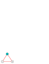
We now derive $h_{rt}(x)$, i.e., the generating function for the number of nodes influenced by following a red triangle selected at random; similar arguments hold for $h_{bt}(x)$. We demonstrate this situation in Figure 3, where the top vertex $u$ is active, and we are interested in computing the generating function for the number of nodes that will be influenced by nodes $v$ and $w$. We will compute the generating function $h_{rt}(x)$ by conditioning on the following events:

Figure 3: Assume that the top vertex $u$ is active in network ${\mathbb{R}}$. Whether it will activate the other two nodes will depend on whether $v$ and/or $w$ are ${\mathbb{R}}$-vulnerable.

• If neither of nodes $v$ and $w$ is ${\mathbb{R}}$-vulnerable, then the number of nodes influenced will be zero. Node $v$ has degree ${{\mathbf{d}}}$ with normalized probability $\frac{n_{rt}{p_{\mathbf{d}}}}{<n_{rt}>}$, in which case it is not ${\mathbb{R}}$-vulnerable with probability $1-\rho_{{{\mathbf{d}}},rs}$. Similarly, the probability that node $w$ has degree ${{\mathbf{d}}}^{\prime}$ and not ${\mathbb{R}}$-vulnerable is $(\frac{n_{rt}^{\prime}{p_{\mathbf{d^{\prime}}}}}{<n_{rt}^{\prime}>})(1-\rho_{{{\mathbf{d^{\prime}}}},rs})$. Summing over all possible cases, we obtain the first term in (7) with $x^{0}$ (meaning that zero nodes will be influenced by following the red triangle in this case).

• Consider the case where only one of $v$ and $w$ is influenced, leading to a term with the factor $x^{1}$ in (7). Without loss of generality, consider the case where $v$ is activated while $w$ is not. If node $v$ has degree ${{\mathbf{d}}}$, then it is ${\mathbb{R}}$-vulnerable with probability $\rho_{{{\mathbf{d}}},rs}$, and can influence other nodes in the usual manner. Then, the event that node $w$, with degree ${{\mathbf{d^{\prime}}}}$, will not be activated despite having two active neighbors (nodes $u$ and $v$) has probability $1-\rho_{{{\mathbf{d^{\prime}}}},rt}$. By symmetry and exchangeability of nodes $v$ and $w$, an equivalent term will be obtained for the case where $w$ is activated but $v$ is not. Summing over all possibilities we obtain the second term in (7).

• Finally, we consider the case where both $v$ and $w$ become active giving rise to term with factor $x^{2}$. There are two possible scenarios:

  • Both of $v$ and $w$ are $actived$ by $u$. The probability that $v$ is $actived$ by $u$ is $\rho_{{{\mathbf{d}}},rs}$ as already discussed during the computation of the first term. By symmetry, the probability for $w$ is the same as for $v$. Multiplying the two probabilities leads to the third term in (7).

  • Only one of $v$ and $w$ is made active immediately by $u$ while the other is not; e.g., say $v$ is activated but not $w$. However, $w$ also gets activated by the joint influence from $u$ and $v$. With ${{\mathbf{d}}}$ and ${{\mathbf{d^{\prime}}}}$ denoting the degree of $v$ and $w$, this happens with probability $(\rho_{{{\mathbf{d}}},rs})(\rho_{{{\mathbf{d^{\prime}}}},rt}-\rho_{{{\mathbf{d^{\prime}}}},rs})$. Here, the second term accounts for the fact that $w$ gets activated only if it has two (or, more) active neighbors. Summing over all possibilities as before, and multiplying by two for the case where $v$ and $w$ are replaced, we obtain the last term in (7).

III.3 Deriving the Condition for Global Cascades

The discussion given in Section III.1 and III.2 leads to a set of recursive equations for $h_{rs}(x)$, $h_{rt}(x)$, $h_{bs}(x)$, and $h_{bt}(x)$. Recursions for $h_{rs}(x)$ and $h_{rt}(x)$ are given in (6) and (7), respectively; the expressions for $h_{bs}(x)$ and $h_{bt}(x)$ are very similar and omitted here for brevity. With these four recursive equations in place, it is possible to determine the characteristic function $H(x)$ of the finite number of nodes activated in the contagion process. Namely, for a given $x$, we shall find a fixed-point of these recursive equations, and then use the resulting values of $h_{rs}(x)$, $h_{rt}(x)$, $h_{bs}(x)$, and $h_{bt}(x)$ in (3) to get $H(x)$.

$$h_{rs}(x) =x\sum_{{{\mathbf{d}}}}\frac{d_{rs}{p_{\mathbf{d}}}}{<d_{rs}>}\rho_{{{\mathbf{d}}},rs}D(d_{rs}-1,n_{rt},d_{bs},n_{bt})+x^{0}\sum_{{{\mathbf{d}}}}\frac{d_{rs}{p_{\mathbf{d}}}}{<d_{rs}>}\left(1-\rho_{{{\mathbf{d}}},rs}\right)$$ (6)

$$h_{rt}(x) =x^{0}\sum_{{{\mathbf{d}}}}\sum_{{{\mathbf{d^{\prime}}}}}\frac{n_{rt}{p_{\mathbf{d}}}}{<n_{rt}>}\left(1-\rho_{{{\mathbf{d}}},rs}\right)\frac{n_{rt}^{\prime}{p_{\mathbf{d^{\prime}}}}}{<n_{rt}^{\prime}>}(1-\rho_{{{\mathbf{d^{\prime}}}},rs})$$ (7)

$$~{}~{}~{}~{}+2x\sum_{{{\mathbf{d}}}}\sum_{{{\mathbf{d^{\prime}}}}}\frac{n_{rt}{p_{\mathbf{d}}}}{<n_{rt}>}\rho_{{{\mathbf{d}}},rs}D(d_{rs},n_{rt}-1,d_{bs},n_{bt})\frac{n_{rt}^{\prime}{p_{\mathbf{d^{\prime}}}}}{<n_{rt}^{\prime}>}\left(1-\rho_{{{\mathbf{d^{\prime}}}},rt}\right)$$

$$~{}~{}~{}~{}+x^{2}\sum_{{{\mathbf{d}}}}\sum_{{{\mathbf{d^{\prime}}}}}\left(\frac{n_{rt}{p_{\mathbf{d}}}}{<n_{rt}>}\rho_{{{\mathbf{d}}},rs}D(d_{rs},n_{rt}-1,d_{bs},n_{bt})\right)\left(\frac{n_{rt}^{\prime}{p_{\mathbf{d^{\prime}}}}}{<n_{rt}^{\prime}>}\rho_{{{\mathbf{d^{\prime}}}},rs}D(d_{rs}^{\prime},n_{rt}^{\prime}-1,d_{bs}^{\prime},n_{bt}^{\prime})\right)$$

$$~{}~{}~{}~{}+2x^{2}\sum_{{{\mathbf{d}}}}\sum_{{{\mathbf{d^{\prime}}}}}\left(\frac{n_{rt}{p_{\mathbf{d}}}}{<n_{rt}>}\rho_{{{\mathbf{d}}},rs}D(d_{rs},n_{rt}-1,d_{bs},n_{bt})\right)\left(\frac{n_{rt}^{\prime}{p_{\mathbf{d^{\prime}}}}}{<n_{rt}^{\prime}>}\left(\rho_{{{\mathbf{d^{\prime}}}},rt}-\rho_{{{\mathbf{d^{\prime}}}},rs}\right)D(d_{rs}^{\prime},n_{rt}^{\prime}-1,d_{bs}^{\prime},n_{bt}^{\prime})\right)$$

By conservation of probability and the definition of generating functions, we know that $H(1)=1$ only if final number of activated nodes is finite with probability one. In other words, global cascades that lead to a positive fraction of influenced nodes are possible only if $H(1)<1$. This prompts us to seek a fixed point of the recursive equations when $x=1$. For notational convenience, we define $h_{1}:=h_{rs}(1)$, $h_{2}:=h_{rt}(1)$, $h_{3}:=h_{bs}(1)$, and $h_{4}:=h_{bt}(1)$. From (3), this gives

$$H(1)=\sum_{{{\mathbf{d}}}}{p_{\mathbf{d}}}h_{1}^{d_{rs}}h_{2}^{n_{rt}}h_{3}^{d_{bs}}h_{4}^{n_{bt}},$$ (8)

while the recursions take the form

$$h_{i}=g_{i}(h_{1},h_{2},h_{3},h_{4}),\quad i=1,2,3,4.$$ (9)

Here the functions $g_{1},g_{2}$ are easily obtained from (6) and (7), and similarly $g_{3}$ and $g_{4}$ can be obtained from the recursions for $h_{bs}(x)$, and $h_{bt}(x)$. To give an example, we have

$$g_{3}(h_{1},h_{2},h_{3},h_{4})$$

$$=\sum_{{{\mathbf{d}}}}\frac{d_{bs}{p_{\mathbf{d}}}}{<d_{bs}>}\left(\rho_{{{\mathbf{d}}},bs}h_{1}^{d_{rs}}h_{2}^{n_{rt}}h_{3}^{d_{bs}-1}h_{4}^{n_{bt}}+1-\rho_{{{\mathbf{d}}},bs}\right)$$

It is clear that the recursions (9) have a trivial fixed point $h_{1}=h_{2}=h_{3}=h_{4}=1$ which yields $H(1)=1$, meaning that cascades will die out without reaching a positive fraction of the population with high probability. However, the trivial solution is the physical solution only if it is a stable fixed point. To check its stability, we linearize the recursive equations (9) around $x=1$, and compute the corresponding Jacobian matrix $\mathbf{J}$ via

$$\mathbf{J}(i,j)=\frac{\partial g_{i}(h_{1},h_{2},h_{3},h_{4})}{\partial h_{j}}\Bigg{|}_{h_{1}=h_{2}=h_{3}=h_{4}=1}$$ (10)

for each $i,j=1,2,3,4$; the exact expression for the four by four matrix $\mathbf{J}$ is not give here in order to save space. Now, the trivial solution $h_{1}=h_{2}=h_{3}=h_{4}=1$ is stable if and only if the largest eigenvalue in absolute value of $\mathbf{J}$, denoted $\sigma(\mathbf{J})$, is less than or equal to one. Otherwise, if $\sigma(\mathbf{J})>1$, then there exists another fixed point for the recursion with $h_{1},h_{2},h_{3},h_{4}<1$, leading to $H(1)<1$. In that case, the probability deficit $1-H(1)>0$ gives the probability that the contagion process reaches infinitely many nodes, i.e., a global spreading event takes place. Collecting, we conclude that the condition of global cascades is given by $\sigma(\mathbf{J})>1$, while the probability of global cascade equals $P_{trig}=1-H(1)$.

IV Expected Cascade Size

Next, we are interested in computing the expected size of global cascades when they take place. Put differently, we will analyze the expected fraction of nodes that will eventually become active as we randomly pick a node in the network and set it active. We follow the approach used in Gleeson and Cahalane (2007); Hackett et al. (2011b); Yağan and Gligor (2012), which has been proven to be an effective way to analyze expected cascade size in networks.

First, consider the network $\mathbb{H}$ as a tree-structure with an arbitrary node selected as the root. Then, label the levels of the tree from $\ell=0$ at the bottom to $\ell=+\infty$ at the top of the tree. Similar to Hackett et al. (2011b); Yağan and Gligor (2012), we assume that nodes begin updating their states starting from the bottom of the tree and proceeding to the top. In other words, we assume that a node at level $\ell$ updates its state only after all nodes at the lower levels $0,1,\dots,\ell-1$ finish updating. We define $q_{rs,\ell}$ as the probability that a node at level $\ell$ of a tree, which is connected to its unique parent by a red single edge, is active given that its parent at level $\ell+1$ is inactive. Then, we consider a pair of nodes at level $\ell$ that together with their parent at level $\ell+1$ form a red triangle. Given that the parent is inactive, we let $q_{rt1,\ell}$ (resp. $q_{rt2,\ell}$) denote the probability that only one (resp. both) of the two child nodes of this triangle is active. We define $q_{bs,\ell}$, $q_{bt1,\ell}$, and $q_{bt2,\ell}$ for blue edges in the same manner.

According to our model, an active node is never deactivated, meaning that $q_{rs,\ell}$, $q_{rt1,\ell}$, $q_{rt2,\ell}$, $q_{bs,\ell}$, $q_{bt1,\ell}$, $q_{bt2,\ell}$ are all non-decreasing. Therefore, they will converge to $q_{rs,\infty}$, $q_{rt1,\infty}$, $q_{rt2,\infty}$, $q_{bs,\infty}$, $q_{bt1,\infty}$, $q_{bt2,\infty}$. Then, the expected cascade size (i.e., the fraction of active individuals) $S$ is given by the probability that the arbitrary selected node at the top of the tree becomes active. In order to computer $S$, we first derive recursive relations for $q_{rs,\ell}$, $q_{rt2,\ell}$, $q_{rt2,\ell}$, $q_{bs,\ell}$, $q_{bt2,\ell}$, $q_{bt2,\ell}$. We have

$$q_{rs,\ell+1} =\sum_{{{\mathbf{d}}}}\frac{d_{rs}{p_{\mathbf{d}}}}{<d_{rs}>}\sum_{i=0}^{d_{rs}-1}\sum_{j=0}^{n_{rt}}\sum_{x=0}^{j}\sum_{m=0}^{d_{bs}}\sum_{n=0}^{n_{bt}}\sum_{y=0}^{n}Q_{\ell}\left[\left(i,j,x,m,y,n\right),(d_{rs}-1,n_{rt},d_{bs},n_{bt})\right]F\left[(i,x,j-x,m,y,n-y),{{\mathbf{d}}}\right]$$

$$q_{rt1,\ell+1} =2\sum_{{{\mathbf{d}}},{{\mathbf{d^{\prime}}}}}\frac{n_{rt}{p_{\mathbf{d}}}}{n_{rt}}\frac{n_{rt}^{\prime}{p_{\mathbf{d^{\prime}}}}}{<n_{rt}^{\prime}>}\sum_{i,i^{\prime}=0}^{d_{rs},d^{\prime}_{rs}}\sum_{j,j^{\prime}=0}^{n_{rt}-1,n^{\prime}_{rt}-1}\sum_{x,x^{\prime}=0}^{j,j^{\prime}}\sum_{m,m^{\prime}=0}^{d_{bs},d^{\prime}_{bs}}\sum_{n,n^{\prime}=0}^{n_{bt},n_{bt}^{\prime}}\sum_{y,y^{\prime}=0}^{n,n^{\prime}}Q_{\ell}\left[\left(i,j,x,m,y,n\right),(d_{rs},n_{rt}-1,d_{bs},n_{bt})\right]$$

$$~{}~{}~{}~{}Q_{\ell}\left[\left(i^{\prime},j^{\prime},x^{\prime},m^{\prime},y^{\prime},n^{\prime}\right),(d^{\prime}_{rs},n^{\prime}_{rt}-1,d^{\prime}_{bs},n^{\prime}_{bt})\right]F\left[(i,x,j-x,m,y,n-y),{{\mathbf{d}}}\right]$$

$$~{}~{}~{}~{}(1-F\left[(i^{\prime},x^{\prime}+1,j^{\prime}-x^{\prime},m^{\prime},y^{\prime},n^{\prime}-y^{\prime}),{{\mathbf{d^{\prime}}}}\right])$$

$$q_{rt2,\ell+1} =\sum_{{{\mathbf{d}}},{{\mathbf{d^{\prime}}}}}\frac{n_{rt}{p_{\mathbf{d}}}}{n_{rt}}\frac{n_{rt}^{\prime}{p_{\mathbf{d^{\prime}}}}}{<n_{rt}^{\prime}>}\sum_{i,i^{\prime}=0}^{d_{rs},d^{\prime}_{rs}}\sum_{j,j^{\prime}=0}^{n_{rt}-1,n^{\prime}_{rt}-1}\sum_{x,x^{\prime}=0}^{j,j^{\prime}}\sum_{m,m^{\prime}=0}^{d_{bs},d^{\prime}_{bs}}\sum_{n,n^{\prime}=0}^{n_{bt},n_{bt}^{\prime}}\sum_{y,y^{\prime}=0}^{n,n^{\prime}}Q_{\ell}\left[\left(i,j,x,m,y,n\right),(d_{rs},n_{rt}-1,d_{bs},n_{bt})\right]$$

$$~{}~{}~{}Q_{\ell}\left[\left(i^{\prime},j^{\prime},x^{\prime},m^{\prime},y^{\prime},n^{\prime}\right),(d^{\prime}_{rs},n^{\prime}_{rt}-1,d^{\prime}_{bs},n^{\prime}_{bt})\right]\bigg{(}F\left[(i,x,j-x,m,y,n-y),{{\mathbf{d}}}\right]F\left[(i^{\prime},x^{\prime}+1,j^{\prime}-x^{\prime},m^{\prime},y^{\prime},n^{\prime}-y^{\prime}),{{\mathbf{d^{\prime}}}}\right]$$

$$~{}~{}~{}~{}+\big{(}F\left[(i,x+1,j-x,m,y,n-y),{{\mathbf{d}}}\right]-F\left[(i,x,j-x,m,y,n-y),{{\mathbf{d}}}\right]\big{)}F\left[(i^{\prime},x^{\prime},j^{\prime}-x^{\prime},m^{\prime},y^{\prime},n^{\prime}-y^{\prime}),{{\mathbf{d^{\prime}}}}\right]\bigg{)}$$

where we define

$$Q_{\ell}\left[\left(i,j,x,m,n,y\right),(d_{1},d_{2},d_{3},d_{4})\right] ={d_{1}\choose i}q_{rs,\ell}^{i}(1-q_{rs,\ell})^{d_{1}-i}{d_{2}\choose j}{j\choose x}q_{rt1,\ell}^{x}q_{rt2,\ell}^{j-x}(1-q_{rt1,\ell}-q_{rt2,\ell})^{d_{2}-j}{d_{3}\choose m}q_{bs,\ell}^{m}$$

$$~{}~{}~{}~{}~{}~{}~{}(1-q_{bs,\ell})^{d_{3}-m}{d_{4}\choose n}{n\choose y}q_{bt1,\ell}^{y}q_{bt2,\ell}^{n-y}(1-q_{bt1,\ell}-q_{bt2,\ell})^{d_{4}-n}$$ (11)

In words, $Q_{\ell}\left[\left(i,j,x,m,n,y\right),(d_{1},d_{2},d_{3},d_{4})\right]$ gives the probability that a node at level $\ell$ with colored degree $(d_{1},2d_{2},d_{3},2d_{4})$ has

• $i$ (resp. $d_{1}-i$) of the $d_{1}$ neighbors connected through red single edges as active (resp. inactive). Similarly, $m$ (resp. $d_{3}-m$) of the $d_{3}$ neighbors connected through blue single edges as active (resp. inactive)

• of the $d_{2}$ red-triangles it participates in, $x$ has one active node, $j-x$ has two active nodes, and $d_{2}-j$ has no active node. Similarly, of the $d_{4}$ blue-triangles it participates in, $y$ has one active node, $n-y$ has two active nodes, and $d_{4}-n$ has no active node

Hence, multiplying $Q_{\ell}\left[\left(i,j,x,m,n,y\right),(d_{1},d_{2},d_{3},d_{4})\right]$ with $F\left[(i,x,j-x,m,y,n-y),{{\mathbf{d}}}\right]$ and summing over all possibilities for ${{\mathbf{d}}}$ and $i,j,x,m,n,y$ gives the probability that the node under consideration turns active. This confirms the first expression above. Second and third terms consider simultaneously a pair of nodes that are part of a red triangle (where the top, i.e., parent, vertex is inactive). Therefore, we first condition on the degrees of these two nodes being ${{\mathbf{d}}}$ and ${{\mathbf{d^{\prime}}}}$ respectively, and consider all possibilities concerning the states (active vs. inactive) of these neighbors. Then for $q_{rt1,\ell+1}$, we realize by symmetry that the desired expression is two times the probability that the node with degree ${{\mathbf{d}}}$ turns active, and despite having one extra active neighbor, the node with degree ${{\mathbf{d^{\prime}}}}$ does not turn active. The fact that first node turns active is incorporated in the expression $(1-F\left[(i^{\prime},x^{\prime}+1,j^{\prime}-x^{\prime},m^{\prime},y^{\prime},n^{\prime}-y^{\prime}),{{\mathbf{d^{\prime}}}}\right])$ by the term $x^{\prime}+1$. For $q_{rt2,\ell+1}$, we proceed similarly and realize that for both nodes to turn active there are two possibilities. The node with degree ${{\mathbf{d}}}$ either turns active regardless of the state of the node with degree ${{\mathbf{d^{\prime}}}}$ (in which case the node with degree ${{\mathbf{d^{\prime}}}}$ will turn active with probability $F\left[(i^{\prime},x^{\prime}+1,j^{\prime}-x^{\prime},m^{\prime},y^{\prime},n^{\prime}-y^{\prime}),{{\mathbf{d^{\prime}}}}\right]$), or it turns active only after the node with degree ${{\mathbf{d^{\prime}}}}$ does.

With the above recursion in place, we compute the final cascade size via

$$S=\sum_{{{\mathbf{d}}}}{p_{\mathbf{d}}}\sum_{i=0}^{d_{rs}}\sum_{j=0}^{n_{rt}}\sum_{x=0}^{j}\sum_{m=0}^{d_{bs}}\sum_{n=0}^{n_{bt}}\sum_{y=0}^{n}Q_{\infty}\left[\left(i,j,x,m,n,y\right),(d_{rs},n_{rt},d_{bs},n_{bt})\right]F\left[(i,x,j-x,m,y,n-y),{{\mathbf{d}}}\right]$$ (12)

Namely, we first solve for the values of $q_{rs,\infty}$, $q_{rt1,\infty}$, $q_{rt2,\infty}$, $q_{bs,\infty}$, $q_{bt1,\infty}$, $q_{bt2,\infty}$ using the recursive equations, and then substitute them into (12) to obtain the expected size of global cascades.

V Numerical Results

V.1 Networks with Doubly Poisson Distributions

In our first simulation study, we use doubly Poisson distribution for the number of single edges and triangles in both networks. Namely, we set

$$p_{st}^{r} =e^{-\lambda_{r,1}}\frac{(\lambda_{r,1})^{s}}{s!}e^{-\lambda_{r,2}}\frac{(\lambda_{r,2})^{t}}{t!},\mbox{ \ s, t = 0, 1, \ldots},$$

$$p_{st}^{b} =e^{-\lambda_{b,1}}\frac{(\lambda_{b,1})^{s}}{s!}e^{-\lambda_{b,2}}\frac{(\lambda_{b,2})^{t}}{t!},\mbox{ \ s, t = 0, 1, \ldots},$$

where $s$ and $t$ are the number of single edges and triangles in the corresponding networks, respectively. Thus, $\lambda_{r,1}$ and $\lambda_{r,2}$ (resp. $\lambda_{b,1}$ and $\lambda_{b,2}$) denote the mean number of single edges and triangles, respectively in ${\mathbb{R}}$ (resp. in ${\mathbb{B}}$).

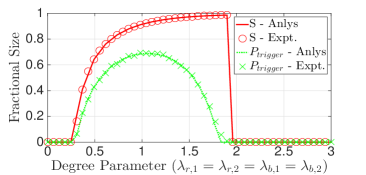
We consider $n=1\times 10^{5}$ nodes in the population and $\alpha=0.5$ for the size of network ${\mathbb{R}}$. We let $\tau=0.18$ and $c=0.25$ for the threshold and content parameters, respectively. The results are shown in Figure 4 where the curves stand for the theoretical results of probability $P_{trig}$ and expected size $S$ of cascades (obtained from our discussion in Section III and IV), as a function of $\lambda_{r,1}=\lambda_{r,2}=\lambda_{b,1}=\lambda_{b,2}$. The markers stand for the empirical results for the same quantities, and are obtained by averaging over 5,000 independent experiments. We see a very good agreement between the analytical and experimental results confirming the validity of our analysis. The slight discrepancy observed in $P_{trig}$ is due to the limited number of experiments, and can be mitigated by increasing the number of realizations.

Figure 4: Simulations for doubly Poisson degree distributions. In (a), we set the content parameter $c=0.25$, the threshold as $\tau=0.18$, and $\alpha=0.5$, and vary the degree parameters. In (b), we fix $\tau=0.18$, $\lambda_{r,1}=\lambda_{r,2}=\lambda_{b,1}=\lambda_{b,2}=0.3$, and $\alpha=0.5$ while varying content parameter $c$.

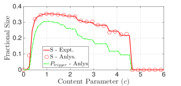
Next, we change our experimental set-up to demonstrate the effect of content parameter on the probability and size of cascades. To that end, we fix all network parameters and observe the quantities of interest as the content parameter $c$ varies. In particular, we set $\lambda_{r,1}=\lambda_{r,2}=\lambda_{b,1}=\lambda_{b,2}=0.3$ and $\tau=0.18$. We see that the probability and expected size of global cascades vary greatly as $c$ changes. This can be taken as an indication that our model can capture the real-world phenomenon that over the same population certain contents can become widespread while others die out quickly. In the setting used here, we see that global cascades take place when the content parameter $c$ is not too small or large. The reason is that with a too small or large content parameter, the connectivity of the conjoined network is dominated by only one of the two networks. So, if neither of them has enough connectivity to trigger a global cascade by their own, then there will be no global cascades in the conjoined network. When the $c$ is neither too large nor too small (e.g., close to unity), both networks will contribute to the connectivity together and it becomes possible to trigger a global cascade. For other values of $\lambda_{r}$ and $\lambda_{b}$ a completely different situation might occur, e.g., with very small or very large $c$ promoting cascades; e.g., see (Yağan and Gligor, 2012, Fig. 2) for a few such examples.

Figure 5: Illustration of the effect of clustering coefficient on the expected cascade and probability of global cascades. We fix $\tau=0.18$, $c=0.25$, and $\alpha=0.5$, then vary the degree parameter $\lambda$ defined in Table 1. We see (a) the probability to trigger a global cascade; (b) the global clustering coefficient introduced in Section II.1; and (c) the expected cascade size.

V.2 How does Clustering Affect the Cascade Size?

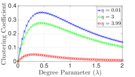
Our next goal is to reveal the impact of clustering on the influence propagation process. In order to control the level of clustering while keeping the mean total degree fixed, we use Poisson distributions for the number of single and triangle edges in two networks with parameters given in Table 1. Obviously, the clustering coefficient in ${\mathbb{R}}$ is fixed while with $\eta\in[0,4]$ the clustering of ${\mathbb{B}}$ varies between the two extremes: i) when $\eta=4$, ${\mathbb{B}}$ will have no single-edges and consist only of triangles resulting with a clustering coefficient close to one; and ii) with $\eta=0$, there will be no triangles in ${\mathbb{B}}$ and hence its clustering coefficient will be close to zero. Collecting, we see that the clustering coefficient of ${\mathbb{B}}$ and thus of ${\mathbb{H}}$ increases with increasing $\eta$ in this setting.

	Network ${\mathbb{R}}$	Network ${\mathbb{B}}$
Distribution of single-edges	Poi($2\lambda$)	2 Poi$(\frac{4-\eta}{2}\lambda)$
Distribution of triangles	Poi($\lambda$)	Poi$\left(\frac{\eta}{2}\lambda\right)$

Table 1: Parameters of the doubly Poisson distribution. This choice ensures that the mean and variance of the total degree distribution (single plus triangle edges) in ${\mathbb{B}}$ are independent of $\eta$, while its clustering varies greatly as $\eta$ varies in $(0,4)$. In Figure 4 we set $\lambda=0.5$.

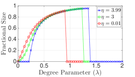
With these in mind, we first demonstrate the impact of clustering on the probability of triggering a global cascade. Figure 5(a) shows the probability of triggering a global cascade as a function of $\lambda$ for three different $\eta$ values. The resulting clustering coefficients are plotted in Figure 5(b) where we clearly see that clustering increases with increasing $\eta$. The main observation from Figure 5(a) is that increasing the clustering (i.e., increasing $\eta$), shifts the interval of $\lambda$ for which global cascades are possible to the right. This leads to a double-faceted conclusion that clustering decreases the probability of global cascades when average degrees are small, whereas after a certain value of average degree, clustering increases the probability of cascades.

The double-faceted impact of clustering on cascade probability can be explained as follows. It is known Watts (2002); Yağan et al. (2013) that threshold models of complex contagion exhibit two phase transitions as the average degree increases, a second-order transition at low degrees that marks the formation of a giant vulnerable component and a first-order transition at high degrees due to increased local stability of nodes; namely, due to the increased difficulty of activating high-degree nodes. Given that clustering is known to decrease the size of giant component Zhuang and Yağan (2016), we expect that it will be more difficult for a clustered network to contain a giant vulnerable cluster. This is why the lower phase transition in complex contagions appear later (i.e., at larger degrees) as clustering increases. On the other hand, the cycles of size three (i.e., triangles) that are common in clustered networks can help trigger cascades when average degree is higher. For instance, in a tree-like network a single active node can only activate its vulnerable connections. However, in a triangle, an active node may first activate one of its vulnerable connections, making it possible for the third node to be activated (which now has two active neighbors) even if it is not vulnerable. This is what pushes the second phase transition to higher degrees.

Next, we explore the impact of clustering on the expected cascade size in Figure 4(c). Here again, we see the double-faceted impact of clustering with small average degrees favoring low clustering, while high degrees favoring high clustering in terms of having a larger cascade size. In fact, we see the existence of a critical average degree (around $\lambda=0.6$ in Figure 4(c)) such that when $\lambda$ is smaller (resp. larger) than the critical value, expected cascade size decreases (resp. increases) with increasing clustering.

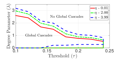
Finally, we consider the impact of clustering on the average degree-cascade threshold plane. For each parameter pair $(\lambda,\tau)$, the curves in Figure 6 separate the region where global cascade can take place (areas inside the boundaries) from the region where they cannot (areas outside the boundaries). Once again, we confirm that increasing the clustering coefficient shifts the interval where cascades are possible up (i.e., to higher degrees) for any threshold $\tau$.

Figure 6: We show the cascade regions in the Degree Parameter-Threshold plane when $\alpha=0.5$, $\tau=0.18$, and both networks follow doubly Poisson distributions as described in Table 1. Clustering increases as $\eta$ increases.

VI Comparison between monoplex and Multiplex Networks

In what follows, we will compare the dynamics of complex contagions over a monoplex network with that over a multiplex network. Of particular interest will be to find out whether the projection of a multiplex network into a monoplex network leads to any significant differences in the dynamics that would warrant the separate analyses of multiplex networks as conducted here.

To identify the factors affecting complex contagions, we consider two different degree distributions to generate the networks. In Section VI.1, we use a setting similar to previous sections, with the resulting networks having almost no degree-degree correlations; e.g., assortativity defined as the Pearson correlation coefficient between the degrees of pairs of linked nodes Newman (2002). In Section VI.2 and VI.3, we use a different setting that leads to (tunable) assortativity for multiplex networks. In order to keep the focus on the comparison between monoplex and multiplex networks, we shall consider only non-clustered networks in the following discussion.

VI.1 Multiplex Networks with Limited Assortativity

First we consider the limited assortativity case and use the following degree distribution to assign blue and red stubs to each node:

$$p_{k}^{b} =e^{-\lambda_{b}}\frac{\lambda_{b}^{k}}{k!},\quad\mbox{ \ k = 0, \ldots},$$ (13)

$$p_{k}^{r} =\alpha e^{-\lambda_{r}}\frac{\lambda_{r}^{k}}{k!}+(1-\alpha)\mathbf{1}[k=0],\quad\mbox{ \ k = 0, \ldots}.$$

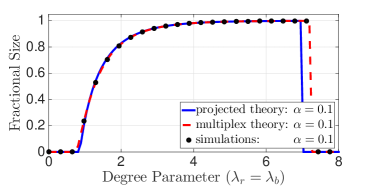
A multiplex network is generated using the colored configuration model Söderberg (2003, 2002) where stubs that are of the same color are matched randomly. The monoplex projected theory ignores the color of the edges and matches all stubs randomly with each other. An important question is whether we lose any significant information about contagion dynamics when the monoplex projected theory is used instead of the multiplex theory developed here and in Yağan and Gligor (2012). For convenience and fair comparison, we set $\lambda_{b}=\lambda_{r}$ and use $c=1$ as the content parameter.

In Figure 7, we set $\alpha=0.99$. We see nearly no difference between the theoretical cascade sizes obtained from monoplex and multiplex theories, and they both match the simulation results well. However, when $\alpha$ is reduced to 0.1 in Figure 7, we clearly see a difference between the two theories and only multiplex theory matches the simulation results. This shows that even in the simplest case where both link types have the same influence factor (i.e., $c=1$), monoplex theory may be unable to capture certain properties of cascade dynamics, reinforcing the need for studying cascades using the multiplex theory.

We now explain why the two cases, $\alpha=0.1$ and $\alpha=0.99$, lead to different conclusions regarding the accuracy of the monoplex theory in capturing contagion dynamics over multiplex networks. One of the key differences between the two cases is the resulting assortativity. In the former case with $\alpha=0.1$, only $10\%$ of the nodes has red stubs, each of which shall be connected with other red stubs in the multiplex network case. Put differently, in this setting a small fraction of the population will have statistically higher degrees than the rest, and the additional links they have can only connect nodes with high degrees together. This leads to a positive correlation (i.e., assortativity) between the degrees of pairs of connected nodes. However, in the monoplex projection, the additional edges can be used to connect any two nodes, resulting with very little to no assortativity in the network. Obviously, when $\alpha$ is close to one, almost every node will have the additional edges and the above phenomenon will not be observed. Our simulation results confirm this intuition as we see that assortativity is negligible ($\sim 10^{-4}$) in both monoplex and multiplex cases when $\alpha=0.99$, while with $\alpha=0.1$, assortativity varies (as $\lambda_{r}=\lambda_{b}$ increases) from $0.05$ to $0.2$ in the multiplex case while still being negligible in the monoplex case.

The impact of assortativity on the comparison between monoplex and multiplex theories is investigated further in the forthcoming discussion.

Figure 7: Comparison between monoplex networks and multiplex networks with limited assortativity. In (a) and (b), we fix the threshold $\tau=0.15$, the content parameter $c=1$, then vary the degree parameters in (13). For the networks obtained by projected theory and the networks in multiplex theory with $\alpha=0.99$, assortativity is negligible. However, when $\alpha=0.1$, the assortativity coefficient of the networks in the multiplex theory become significant; e.g., it can be up to 0.21.

VI.2 Multiplex Networks with Assortativity

In this section, we change the setting slightly to generate multiplex networks with high assortativity. To that end, we use the degree distributions given at (13), but instead of setting $\lambda_{r}=\lambda_{b}$, we enforce

$$\alpha\lambda_{r}=\lambda_{b}$$ (14)

for any $\alpha\in(0,1)$. This setting allows us to tune assortativity without changing the mean degree in the network. In particular, assortativity will increase as $\alpha$ decreases (by virtue of a small fraction of nodes forming a highly-connected cluster) Zhuang and Yağan (2016). In addition, this setting allows us to compare the contagion dynamics in multi-layer networks when the upper layer is i) small but densely connected (small $\alpha$) versus ii) large but loosely connected (large $\alpha$); see Zhuang and Yağan (2016) for relevant results for bond percolation processes.

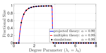
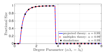
Using the above degree distributions, we generate monoplex and multiplex networks as in Section VI.1 and analyze the complex contagion process. In Figure 8, we see that when $\alpha=0.99$, which leads to very limited assortativity, the difference between monoplex and multiplex networks is negligible. This is in parallel with what we observed in Section VI.1. However, decreasing $\alpha$ to 0.1 leads to two interesting observations in Figure 8. First, instead of the commonly reported two phase transitions Watts (2002); Yağan et al. (2013), we observe four phase transitions in the cascade size as $\alpha\lambda_{r}=\lambda_{b}$ increases. Secondly we see a significant difference between the monoplex projected theory and multiplex theory, with multiplex theory matching the simulations perfectly. Once again, this shows that monoplex theory is unable to capture the cascade dynamics under certain settings.

Figure 8: Comparison between monoplex networks and multiplex networks with assortativity. Similar with the observation in Figure 7, networks in the projected theory and in the multiplex theory with $\alpha=0.99$ have negligible assortativity coefficients. However, for the networks of multiplex theory with $\alpha=0.1$, assortativity coefficient ranges from $0.19$ to $0.79$. In general, assortativity increases with increasing $\lambda_{r}$ and $\lambda_{b}$ in the multiplex theory.

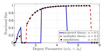
The emergence of four phase transitions in Figure 8, which to the best of our knowledge was not reported before, can be explained as follows. When $\alpha=0.1$, only ten percent of the nodes have red edges, but the the mean number of red edges for those nodes equals $10\lambda_{b}$ (see (14)). Therefore, the first couple of phase transitions taking place at very small $\lambda_{b}$ values can be attributed mainly to red-edges. First, $\lambda_{b}$ becomes large enough (e.g., gets to around 0.1) that the sub-network induced only on the red-edges contains a giant vulnerable cluster, giving rise to global cascades; note that at this point $\lambda_{b}$ is so small that blue edges do not create enough local stability to prevent cascades from happening. However, after $\lambda_{b}$ reaches a certain level (around $0.65$), the subgraph on red-edges, having average degree of $10\lambda_{b}$, reaches the second phase transition point where cascades stop due to the increased local connectivity of nodes. These first two transitions being second- and first-order, respectively, also confirms that they are primarily due to the red-edges.

As $\lambda_{b}$ increases further we observe an interval where there are no global cascades due to either colors of edges; nodes with red and blue-edges are highly stubborn while nodes with only blue edges are not connected enough to trigger a cascade. This interval is then followed by a region where $\lambda_{b}$ is large enough that the sub-graph on blue edges has a giant vulnerable cluster. However, the emergence of a second-order transition in the whole network is prevented here due to some of these nodes turning stubborn as a result of their red-edges. Eventually, however, $\lambda_{b}$ becomes large enough that even with occasional stubborn nodes present, a giant vulnerable cluster emerges. This point is reached much later in monoplex networks as compared to the multiplex networks. This is because in the former case stubborn nodes (with red edges) are equally likely to be connected with any other node, while in the latter case they are mostly connected with each other; thus in the latter case they are less likely to inhibit the emergence of a giant vulnerable cluster on blue edges.

Finally, the system goes through a fourth transition when $\lambda_{b}$ becomes large enough that even nodes with only blue edges become highly connected and hence stubborn. We see that this final transition point is reached much later in multiplex networks than monoplex networks meaning that cascades take place over a broader range of $\lambda_{b}$ values in the former case. Again, this can be attributed to the high assortativity seen in multiplex networks that leads to extremely stubborn nodes (that have both blue and red edges) being isolated from those that are mildly stubborn (that have only blue edges). On the other hand, in monoplex networks, every node is able to connect with the extremely stubborn nodes, and thus the critical value of $\lambda_{b}$ at which cascades become impossible due to high local stability is reached much earlier than that in multiplex networks.

VI.3 Two vs. Four Phase Transitions

In Section VI.2, we have observed the possibility of having more than two phase transitions in the cascade size. As discussed there, multiple phase transitions occur mainly due to the setting (14) that, with small $\alpha$, ensures a small fraction of nodes having significantly higher connectivity than the rest, while also being mostly connected with each other. Since the existence of more than two transitions has not been reported in previous studies, we are interested in exploring it further. In particular, we now investigate the impact of $\alpha$ on the number of phase transitions as well as transition points. Of particular interest will be to find the critical $\alpha$ value that separates the cases where four phase transitions occur from those with only two transitions; e.g., the $\alpha$ value for which the two cascade regions overlap. For simplicity we only consider multiplex networks in this section.

Figure 9: Demonstration of multiple phase transitions.

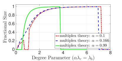
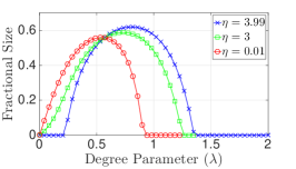
Figure 9 shows the expected size of global cascades under (13)-(14) for three different values of $\alpha$. We see that global cascades take place over a single interval of $\alpha\lambda_{r}=\lambda_{b}$ when $\alpha$ is large (e.g., $\alpha=0.99$) while over two disjoint intervals when $\alpha$ is small (e.g., $\alpha=0.1$). When $\alpha$ is somewhere in between (e.g., case $\alpha=0.166$ ) it is possible to have the cascade intervals partially overlap. In such cases, we only see a single interval where global cascades take place. However, an additional transition point appears, manifested by a shift of slope in cascade size, marking possibly the overlapping point of (what would be) the two cascade intervals.

Figure 9 allows us to comment also on the impact of the size and density of the overlaying social network in facilitating influence propagation. With (14) in effect, a small $\alpha$ corresponds to a social network with few but densely connected individuals, while large $\alpha$ corresponds to a social network with many subscribers, each with few connections on average. In all cases, the total number of edges in the social network is fixed by virtue of (14). We see from Figure 9 that the comparison between the three cases leads to a multi-faceted picture as the mean number of links $\alpha\lambda_{r}$ varies. For instance, the large but loosely connected case of $\alpha=0.99$ leads to the largest expected global cascade size over a certain interval, but it has the smallest cascade interval among all three. The intermediate case of $\alpha=0.166$ seems like a stretched version (over the $x$-axis) of the case with $\alpha=0.99$. In particular, this case leads to the largest interval where global cascades are possible, though the expected cascade size is smaller than that obtained with $\alpha=0.99$ (and also with $\alpha=0.1)$ over certain intervals. Finally, the case of a small but densely connected overlay (i.e., with $\alpha=0.1$), falls right under the case with $\alpha=0.166$ for most values of $\alpha\lambda_{r}$, though it gives the largest size of all three in small intervals where $\alpha\lambda_{r}$ is very small or very large.

VII Conclusion and Future Work

We studied the diffusion of influence in clustered multiplex networks. We solved analytically for the condition, probability, and expected size of global cascades, and confirmed our results via extensive computer simulations. One of our key findings is to show how clustering affects the probability and expected size of global cascades. We also compared several interesting properties of complex contagions on a multiplex network and its monoplex projection. We demonstrate that ignoring link types and aggregating network layers may lead to inaccurate conclusions about contagion dynamics, particularly when assortativity is high. Finally, we show for the first time that linear threshold models do not necessarily exhibit two phase transitions as previously reported. Depending on assortativity, we show that both in monoplex and multiplex cases (with two link types) it is possible to observe four phase transitions.

Our analysis and modeling framework subsumes some previous studies. For instance, by setting $h_{rt}(x)=h_{bt}(x)=1$ in the recursive relations, we ensure that ${\mathbb{R}}$ and ${\mathbb{B}}$ are non-clustered random networks. So, our analysis corresponds to complex contagions in non-clustered networks, which was studied in Yağan and Gligor (2012). Similarly, if we let $h_{rs}(x)=h_{rt}(x)=1$ in the recursions and set the content parameter $c=1$, then our analysis corresponds to complex contagions in clustered monoplex networks, which was studied in Hackett et al. (2011b).

Future work may consider in more details the impact of assortativity or other topological features on the cascade dynamics. It would also be interesting to compare multiplex networks and their monoplex projections in terms of other dynamical processes; e.g., site percolation, transport processes, etc.

References

- Buldyrev et al. (2010) S. V. Buldyrev, R. Parshani, G. Paul, H. E. Stanley, and S. Havlin, Nature 464, 1025 (2010).
- Vespignani (2010) A. Vespignani, Nature 464, 984 (2010).
- Yağan et al. (2012) O. Yağan, D. Qian, J. Zhang, and D. Cochran, IEEE Transactions on Parallel and Distributed Systems 23, 1708 (2012), arXiv:1201.2698v2.
- Brummitt et al. (2012a) C. D. Brummitt, R. M. D’Souza, and E. Leicht, Proceedings of the National Academy of Sciences 109, E680 (2012a).
- Radicchi and Arenas (2013) F. Radicchi and A. Arenas, Nature Physics 9, 717 (2013).
- Reis et al. (2014) S. D. Reis, Y. Hu, A. Babino, J. S. Andrade Jr, S. Canals, M. Sigman, and H. A. Makse, Nature Physics 10, 762 (2014).
- Albert et al. (2000) R. Albert, H. Jeong, and A.-L. Barabási, nature 406, 378 (2000).
- Cohen et al. (2000) R. Cohen, K. Erez, D. Ben-Avraham, and S. Havlin, Physical review letters 85, 4626 (2000).
- Cohen et al. (2002) R. Cohen, D. Ben-Avraham, and S. Havlin, Physical Review E 66, 036113 (2002).
- Leicht and D’Souza (2009) E. Leicht and R. M. D’Souza, arXiv preprint arXiv:0907.0894 (2009).
- Nagler et al. (2011) J. Nagler, A. Levina, and M. Timme, Nature Physics 7, 265 (2011).
- Murray (2002) J. D. Murray, Mathematical Biology, 3rd ed. (Springer, New York (NY), 2002).
- Son et al. (2011) S.-W. Son, P. Grassberger, and M. Paczuski, Physical review letters 107, 195702 (2011).
- Baxter et al. (2012) G. Baxter, S. Dorogovtsev, A. Goltsev, and J. Mendes, Physical review letters 109, 248701 (2012).
- Dickison et al. (2012) M. Dickison, S. Havlin, and H. E. Stanley, Physical Review E 85, 066109 (2012).
- Anderson and May (1991) R. M. Anderson and R. M. May, Infectious Diseases of Humans (Oxford University Press, Oxford (UK), 1991).
- Sahneh et al. (2013) F. Sahneh, C. Scoglio, and P. Van Mieghem, Networking, IEEE/ACM Transactions on 21, 1609 (2013).
- Yağan et al. (2013) O. Yağan, D. Qian, J. Zhang, and D. Cochran, IEEE Journal on Selected Areas in Communications 31, 1038 (2013).
- Valdez et al. (2013) L. D. Valdez, P. A. Macri, H. E. Stanley, and L. A. Braunstein, Physical Review E 88, 050803 (2013).
- Zhao and Bianconi (2013) K. Zhao and G. Bianconi, Journal of Statistical Mechanics: Theory and Experiment 2013, P05005 (2013).
- Cellai et al. (2013) D. Cellai, E. López, J. Zhou, J. P. Gleeson, and G. Bianconi, Physical Review E 88, 052811 (2013).
- Azimi-Tafreshi et al. (2014) N. Azimi-Tafreshi, J. Gómez-Gardeñes, and S. Dorogovtsev, Physical Review E 90, 032816 (2014).
- Bianconi and Dorogovtsev (2014) G. Bianconi and S. N. Dorogovtsev, Physical Review E 89, 062814 (2014).
- Radicchi (2015) F. Radicchi, Nature Physics 11, 597 (2015).
- Gleeson (2008) J. P. Gleeson, Physical Review E 77, 046117 (2008).
- Watts (2002) D. J. Watts, Proceedings of the National Academy of Sciences 99, 5766 (2002).
- Yağan and Gligor (2012) O. Yağan and V. Gligor, Physical Review E 86, 036103 (2012).
- Hackett et al. (2016) A. Hackett, D. Cellai, S. Gómez, A. Arenas, and J. P. Gleeson, Phys. Rev. X 6, 021002 (2016).
- Zhuang and Yağan (2016) Y. Zhuang and O. Yağan, IEEE Transactions on Network Science and Engineering PP, 1 (2016).
- Brummitt et al. (2012b) C. D. Brummitt, K.-M. Lee, and K.-I. Goh, Physical Review E 85, 045102 (2012b).
- Kivelä et al. (2014) M. Kivelä, A. Arenas, M. Barthelemy, J. P. Gleeson, Y. Moreno, and M. A. Porter, Journal of complex networks 2, 203 (2014).
- De Domenico et al. (2014) M. De Domenico, A. Solé-Ribalta, S. Gómez, and A. Arenas, 111, 8351 (2014).
- De Domenico et al. (2013) M. De Domenico, A. Solé-Ribalta, E. Cozzo, M. Kivelä, Y. Moreno, M. A. Porter, S. Gómez, and A. Arenas, Physical Review X 3, 041022 (2013).
- Min et al. (2014) B. Min, S. Do Yi, K.-M. Lee, and K.-I. Goh, Physical Review E 89, 042811 (2014).
- Serrano et al. (2015) M. Á. Serrano, L. Buzna, and M. Boguñá, New Journal of Physics 17, 053033 (2015).
- Granell et al. (2013) C. Granell, S. Gómez, and A. Arenas, Physical review letters 111, 128701 (2013).
- Baxter et al. (2014) G. J. Baxter, S. N. Dorogovtsev, J. F. F. Mendes, and D. Cellai, Physical Review E 89, 042801 (2014).
- De Domenico et al. (2016) M. De Domenico, C. Granell, M. A. Porter, and A. Arenas, arXiv preprint arXiv:1604.02021 (2016).
- Wu et al. (2016) H. Wu, A. Arenas, and S. Gómez, arXiv preprint arXiv:1606.01688 (2016).
- Boccaletti et al. (2014) S. Boccaletti, G. Bianconi, R. Criado, C. I. Del Genio, J. Gómez-Gardeñes, M. Romance, I. Sendiña-Nadal, Z. Wang, and M. Zanin, Physics Reports 544, 1 (2014).
- Cellai and Bianconi (2016) D. Cellai and G. Bianconi, Physical Review E 93, 032302 (2016).
- Newman et al. (2001) M. E. Newman, S. H. Strogatz, and D. J. Watts, Physical review E 64, 026118 (2001).
- Newman (2003) M. E. Newman, SIAM review 45, 167 (2003).
- Watts and Strogatz (1998) D. J. Watts and S. H. Strogatz, Nature 393, 440 (1998).
- Serrano and Boguñá (2006) M. A. Serrano and M. Boguñá, Phys. Rev. E 74, 056114 (2006).
- Newman (2009) M. E. J. Newman, Physical review letters 103, 058701 (2009).
- Gleeson et al. (2010) J. P. Gleeson, S. Melnik, and A. Hackett, Physical Review E 81, 066114 (2010).
- Hackett et al. (2011a) A. Hackett, J. P. Gleeson, and S. Melnik, Int. J. Complex Systems in Science 1, 25 (2011a).
- Hackett et al. (2011b) A. Hackett, S. Melnik, and J. P. Gleeson, Physical Review E 83, 056107 (2011b).
- Huang et al. (2013) X. Huang, S. Shao, H. Wang, S. V. Buldyrev, H. E. Stanley, and S. Havlin, EPL (Europhysics Letters) 101, 18002 (2013).
- Colomer-de Simón and Boguñá (2014) P. Colomer-de Simón and M. Boguñá, Physical Review X 4, 041020 (2014).
- Cozzo et al. (2015) E. Cozzo, M. Kivelä, M. De Domenico, A. Solé-Ribalta, A. Arenas, S. Gómez, M. A. Porter, and Y. Moreno, New Journal of Physics 17, 073029 (2015).
- Miller (2009) J. C. Miller, Physical Review E 80, 020901 (2009).
- Molloy and Reed (1995) M. Molloy and B. Reed, Random structures & algorithms 6, 161 (1995).
- Tang et al. (2011) S. Tang, J. Yuan, X. Mao, X.-Y. Li, W. Chen, and G. Dai, in Proceedings of IEEE INFOCOM 2011 (2011) pp. 2291 –2299.
- Dodds and Watts (2004) P. Dodds and D. J. Watts, Phys. Rev. Lett. 92, 218701 (2004).
- Athreya and Ney (2012) K. B. Athreya and P. E. Ney, Branching processes, Vol. 196 (Springer Science & Business Media, 2012).
- Wilf (2013) H. S. Wilf, generatingfunctionology (Elsevier, 2013).
- Gleeson and Cahalane (2007) J. P. Gleeson and D. J. Cahalane, Physical Review E 75, 056103 (2007).
- Newman (2002) M. E. Newman, Physical review letters 89, 208701 (2002).
- Söderberg (2003) B. Söderberg, Physical Review E 68, 015102 (2003).
- Söderberg (2002) B. Söderberg, Physical review E 66, 066121 (2002).