Flocking dynamics with voter-like interactions

Abstract

We study the collective motion of a large set of self-propelled particles subject to voter-like interactions. Each particle moves on a two-dimensional space at a constant speed in a direction that is randomly assigned initially. Then, at every step of the dynamics, each particle adopts the direction of motion of a randomly chosen neighboring particle. We investigate the time evolution of the global alignment of particles measured by the order parameter $\varphi$, until complete order $\varphi=1.0$ is reached (polar consensus). We find that $\varphi$ increases as $t^{1/2}$ for short times and approaches exponentially fast to $1.0$ for long times. Also, the mean time to consensus $\tau$ varies non-monotonically with the density of particles $\rho$, reaching a minimum at some intermediate density $\rho_{\mbox{\tiny min}}$. At $\rho_{\mbox{\tiny min}}$, the mean consensus time scales with the system size $N$ as $\tau_{\mbox{\tiny min}}\sim N^{0.765}$, and thus the consensus is faster than in the case of all-to-all interactions (large $\rho$) where $\tau=2N$. We show that the fast consensus, also observed at intermediate and high densities, is a consequence of the segregation of the system into clusters of equally-oriented particles which breaks the balance of transitions between directional states in well mixed systems.

1 Introduction

Imitation is one of the a fundamental social mechanisms implemented in most statistical physics models of opinion formation [1]. By means of local pairwise interactions between agents, the imitation mechanism generates an ordering dynamics that allows to study how a population of individuals reaches consensus, i e., a state where all individuals share the same opinion. Among the most studied opinion formation models, the so-called voter model (VM) is the most basic model that introduces social imitation in a simple way. In its original formulation [2, 3], each individual or voter is located at the site of a $d$-dimensional lattice and can take one of two possible opinions represented by an up or a down spin ($S=\uparrow$ or $\downarrow$). At each time step of the dynamics, a voter chosen at random simply adopts the opinion of a randomly chosen nearest neighbor. This local alignment dynamics leads to the formation of same-spin domains that growth in size until one domain takes over the entire lattice and the system reaches consensus in a time that scales as $N^{2}$, $N\ln N$ and $N$ in one, two and three dimensions, respectively [4, 5]. This ultimate state is frozen as spins cannot longer evolve. The macroscopic dynamic behavior of the VM can be understood in terms of its associated Langevin equation for the magnetization field [6, 7], whose Ginzburg-Landau potential is zero. The VM with an arbitrary number of opinion states (the multi-state Voter Model) has recently been studied in [8, 9], where the authors found interesting properties on the evolution of the number of different opinions and the consensus times. The VM has also been applied to the study of other processes like kinetics of heterogeneous catalysis [4, 5], species competition [2] and ecological diversity [10, 11, 12]. Several extensions of the VM have been investigated in the literature, including the presence of zealots or inhomogeneities [13], constrained interactions [14], non-equivalent states [15], asymmetric transitions or bias [16], noise [17] and memory effects [18, 19, 20, 21], among others.

While all these works assumed that agents are fixed in space, some recent works have considered the case in which agents are allowed to move. In reference [22] Sousa et al. introduced mobility in the Sznadj Model for opinion formation and found that consensus is always reached given that agents’ diffusion remove the typical frustrations observed in the static case. Terranova et al. [23] studied a multi-state opinion model with moving individuals and showed that low motility enhances the tendency of the population to adopt moderate states. Lipowska and Lipowski [24] explored the influence of migrations in language formation by means of a model called Naming Game in which agents move diffusively on a two-dimensional (2D) lattice, finding that the language of agents with lowest mobility is favored and that consensus is slower than in systems without motility.

The models described above assume that the direction of motion of a given particle is independent on its opinion or language state. However, in some other social phenomena like the flocking behavior of large groups of animals such as bird flocks, fish schools or insects swarm (see [25, 26, 27] for recent reviews), the direction of motion of each individual is given by its opinion or decision. For instance, Couzin et al. [28] combined experiments and theory to study collective decision making in fish schools. In these experiments, a group of fish is released in a pool and then each fish decides whether to go to a yellow or a blue target. Starting from a minority group trained to have a strong preference for a given target and that is able to persuade the majority group, they showed that the addition of a large enough group of uninformed individuals can promote democratic consensus, returning the control to the majority. In one of the seminal works that connected the field of swarming behavior with that of opinion formation [29] the authors introduced an non-spatial adaptive network approach to model swarming experiments with locusts on a ring-shaped arena [30]. Agents were endowed with one of two possible states (right or left) representing the two possible moving directions of each locust (clockwise and anti-clockwise), and updated their states by interacting with their neighbors in the network. The model reproduced qualitatively the collective properties observed in the experiment, such as a spontaneous symmetry breaking and a density-driven order-disorder transition.

In this article we explore the mechanism of social imitation in flocking dynamics, where the direction of motion of each particle is associated to its opinion state. We propose and study a simple two-dimensional flocking model with voter-like interactions in which, in a single iteration step, each particle adopts the direction of one particle chosen at random within its interacting neighborhood. Unlike the models studied in [28] and [29] and other related models [31], where the possible moving options are binary, all possible directions in the range $(-\pi,\pi]$ are allowed in our model. Besides, interactions are not of mean-field type as in [29], but rather take into account the distance between nearby particles in an euclidean $2D$ space. If we think in the example of a flock of birds, the imitation rule can be interpreted as each bird copying the direction of one close-by bird even if it is able to see a group of, for instance, $10$ birds around. Some recent works have also implemented other types of social interactions to study flocking, like the majority rule dynamics explored in [32], where interactions are not pairwise as in our model but they include a group of neighbors as in the Standard Vicsek Model (SVM) [33]. Also, the model proposed by Chou and Ihle [34] considered the low density limit of the SVM where particles interact by pairs and both take their average orientations, unlike in our model where only one of the two particles updates its direction. We want to note as well that the flocking voter model (FVM) proposed here can be framed as a particular type of coevolving network model [35, 36, 37], in which the network of interactions evolve as particles enter and leave the interaction range of other particles.

We show in this article that the ordering dynamics of the FVM is much slower than that in the SVM. Also, the interplay between the interaction pattern and the alignment dynamics leads to a relaxation to the final ordered state that largely deviates from the one observed in mean-field, as well as in lattices with static particles. As a consequence, the mean time to reach full polar order (consensus) exhibits a non-monotonic dependence with the density of particles. The motion appears to accelerate the polar consensus by a non-trivial mechanism that breaks the equivalence between particle states typically observed in the voter dynamics, introducing a net drift from minority to majority states.

The article is organized as follows. We introduce the model and its dynamics in section 2. In section 3 we explore the ordering dynamics. We analyze the consensus times to the final ordered state in section 4. Finally, we discuss the results and state the conclusions in section 5.

2 The Model

We consider a set of $N$ particles that move on a continuous two-dimensional space $[0,L]^{2}$ with periodic boundary conditions. The density of particles $\rho=N/L^{2}$ is conserved at all times. At a given time $t$, the position of particle $i$ is denoted by $\vec{r_{i}}^{t}=(x_{i}^{t},y_{i}^{t})$ and its velocity by $\vec{v_{i}}^{t}=(v\cos\theta_{i}^{t},v\sin\theta_{i}^{t})$, with speed $|\vec{v_{i}}|=v$ and direction $\theta_{i}^{t}$, for $i=1,..,N$. That is, all particles move at the same speed $v$ but not necessarily in the same direction. At each time step of length $\Delta t=1$, each particle $i$ selects a random neighboring particle $j$ inside a circular region of radius $R=1$ centered at $\vec{r_{i}}$, and updates its position and direction according to

$$\vec{r_{i}}^{t+1} = r_{i}^{t}+\vec{v_{i}}^{t}\Delta t,$$ (1a)

$$\theta_{i}^{t+1} = \theta_{j}^{t},$$ (1b)

where $\theta_{j}^{t}$ is the direction of the particle $j$ at time $t$. In case particle $i$ has no neighbors inside the interaction range $R$, then its direction is not changed. At $t=0$, positions of particles are assigned randomly with a uniform distribution inside the box $[0,L]^{2}$, while their directions are randomly chosen from the interval $(-\pi,\pi]$. Then, each particle moves at a constant speed following a given straight path and can update its direction at integer times $t=1,2,3,...$, by adopting the direction of a neighbor chosen at random. We mention that we are choosing in our model the updating rule used in the original version of the Vicsek model [33], which is known under the name of backward update. In the backward update the velocity at time $t$ is used to obtain the position of a particle at the next time $t+1$ (Eq. 1a), whereas in the forward update that position is obtained using the velocity at time $t+1$. This ambiguity in the selection of the position update and their consequences in the dynamics of the Vicsek model were discussed in some works (see for instance [38]). However, we expect the qualitative behavior of the FVM to be the same under both updates at low speeds. Qualitative differences may appear at high speeds where the difference between moving a particle before or after adopting a direction could be very large in some cases.

3 Ordering dynamics

Voter-like interactions in the dynamics of the model tend to align the direction of neighboring particles. This leads to a local order in the short run, and to global or macroscopic polar order in the long run, as it happens in flocking models with ferromagnetic interactions like the SVM. The ordering properties in these systems are characterized by the parameter $\varphi$, defined as

$$\varphi\equiv\frac{1}{v\,N}\left|\sum_{i=1}^{N}\vec{v_{i}}\right|,$$ (1b)

which is the absolute value of the normalized mean velocity of all particles. The order parameter $\varphi$ can vary from $0$ (total disorder) to $1.0$ (full order).

Figure 1: (Color online) Time evolution of the average order parameter $\left<\varphi\right>$ in a system with $N=4000$ particles, with speed $v=0.1$. Blue (upper) symbols correspond to results of the SVM at zero noise for particle densities $\rho=21$ (triangles) and $\rho=5$ (diamonds). Red (lower) symbols are results for the FVM with densities $\rho=5$ (squares) and $\rho=21$ (circles). The solid line is the theoretical approximation Eq. (1j), while the dashed lines are guides to the eye with slope $1/2$.

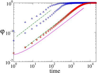
In Fig. 1 we show the temporal behavior of the average value of the order parameter $\left<\varphi\right>$ for speed $v=0.1$, and two different densities. Averages were done over $10^{4}$ independent realizations of the dynamics, as in most plots shown the article unless stated. The two lower curves correspond to the FVM. We also show, for comparison, $\left<\varphi\right>$ for the SVM at zero noise (two upper curves). We observe that, in all cases, full order $\varphi=1.0$ is eventually achieved in the long run. In this final ordered state all particles move in the same direction, thus no more direction updates are possible. Although this final state is not frozen because particles continue moving, it is analogous to the consensus state in the VM. The ordering in the FVM is characterized by an initial increase of $\left<\varphi\right>$ as a power law in time, with an exponent close to $1/2$ (lower dashed line) and a final exponential approach to $1.0$. Even though the approach to complete order in the FVM is much slower than that in the noiseless SVM, we see that the SVM also exhibits an initial algebraic increase of $\left<\varphi\right>$ with time, with an exponent similar to $1/2$ (upper dashed line).

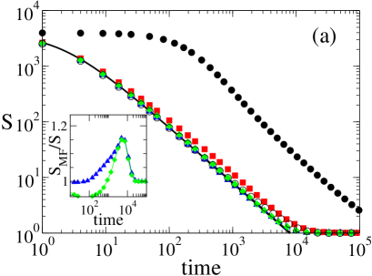
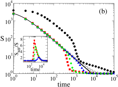
As we see below, the behavior of $\varphi$ is closely related to that of the mean number of different directions $S(t)$ at time $t$ shown in Fig. 2. Initially, all directions are different as they are randomly assigned, and thus $S(t=0)=N$. Then, for densities $\rho\geq 2$ we see that $S$ decreases very slowly during an initial transient of order $N$, as

$$S(t)\simeq\frac{N}{1+t/2},$$ (1c)

represented by a solid line in Fig. 2. This result was derived analytically in [8] following a Master Equation approach and in [9] using generating functions, for the multi-state voter model under sequential update on a complete graph (all-to-all interactions). In the synchronous version of the model that we use here time is rescaled by a factor $1/2$. In the final regime $S$ relaxes exponentially fast to $1.0$, corresponding to the single direction of full order (see Fig. 2). We note that the decrease of $S$ is monotonic at all times. This is because some directions may not be copied by any particle in a single step (mainly those directions followed by few particles), and thus these directions disappear from the system. Then, given that new directions are never created in the voter dynamics, $S$ just decreases monotonically with time.

Solid lines in Fig. 2 correspond to Eq. (1c), which reproduces quite well the evolution of $S$ from simulations on a fully-connected system (all-to-all interactions), represented by empty circles. We also see that these mean-field (MF) curves agree very well with simulations on 2D for large particle densities. Indeed, as the box’s length $L=\sqrt{N/\rho}$ decreases with $\rho$, the MF limit of all-to-all interactions is achieved as $\rho\to\infty$, independent on $v$, because $L$ approaches the interaction range $R=1$. Deviations from MF are evident for very low values of $\rho$ (see $\rho=0.06$ curve), where the number of neighbors is very small and local interactions rule the dynamics. We also observe that for low speed $v=0.1$ [Fig. 2(a)] the agreement between MF and 2D is quite good for $\rho\geq 2$, but for high speeds $v=20$ [Fig. 2(b)] 2D results depart from the MF curve at a time around $10^{3}$. We shall discuss this fast decay of $S$ for large speeds in section 4.

Figure 2: Mean number of different directions $S$ vs time for a system of $N=4000$ particles, speeds $v=0.1$ (a) and $v=20$ (b), and densities $\rho=0.06$ (circles), $2$ (squares), $5$ (diamonds) and $50$ (triangles). Empty circles correspond to numerical results of $S$ on a fully-connected system ($S_{\mbox{\tiny MF}}$), while solid lines are the analytical expression Eq. (1c). Insets: Plots of $\frac{S_{\mbox{\tiny MF}}(t)}{S(t)}$ as function of time for densities $\rho=5$ and $50$ in panel (a), and $\rho=2$, $5$ and $50$ in panel (b). The peaks of the curves make evident the departure of the FVM dynamics from the mean field case.

An approximate expression for the relation between $\varphi$ and $S$ can be obtained by assuming that the directions of particles are randomly distributed at all times, as we describe below. Even though this assumption is only strictly valid at $t=0$ we shall see that it also works reasonable well for longer times. Let’s consider that, at a given time $t$, there are $S(t)$ different independent directions in the system of particles, drawn uniformly in the $(-\pi,\pi]$ range. The number of different directions at time $t$ may vary between realizations, but here we assume that they are all equal to its mean number $S(t)$. Then, we can rewrite the order parameter at time $t$ from Eq. (1b) in the form

$$\varphi(t)=\frac{1}{v\,N}\left|\sum_{k=1}^{S(t)}n_{k}(t)\,\vec{v_{k}}\right|,$$ (1d)

where the sum is over the different particles’ directions $\theta_{k}^{t}$ labeled by the index $k$, which runs from $1$ to its total number $S(t)$. The number of particles moving in the direction $\theta_{k}^{t}$ is denoted by $n_{k}(t)$ and is normalized at all times $\left(\sum_{k=1}^{S(t)}n_{k}(t)=N\right)$. As particles are initially assigned random directions, we have that $S(0)=N$ and $n_{k}(0)=1$ for all $k=1,..,N$. The evolution of the occupation numbers $n_{k}$ is not trivial, thus we make an approximation and assume that at all times $t>0$ they are all equal to its mean value $n_{k}(t)\simeq N/S(t)$ ($k=1,..,S$). Therefore, Eq. (1d) can be written as

$$\varphi(t)\simeq\frac{1}{v\,S(t)}\left|\sum_{k=1}^{S(t)}\vec{v_{k}}\right|=|\vec{V}|,$$ (1e)

where we have defined the resulting vector $\vec{V}\equiv\frac{1}{v\,S(t)}\sum_{k=1}^{S(t)}\vec{v_{k}}$. Given the assumption that all velocities $\vec{v_{k}}$ are independent and uniformly distributed in $(-\pi,\pi]$, the respective $x$ and $y$ components of $\vec{V}$, $V_{x}$ and $V_{y}$, are uncorrelated. Then, from the central limit theorem we know that, in the $S\gg 1$ limit, $V_{x}$ and $V_{y}$ are normally distributed with zero mean ($\langle V_{x}\rangle=\langle V_{y}\rangle=0$)

$$P(V_{x})=\frac{1}{\sqrt{2\pi}\sigma_{x}}e^{-\frac{V_{x}^{2}}{2\sigma_{x}^{2}}},~{}~{}~{}~{}P(V_{y})=\frac{1}{\sqrt{2\pi}\sigma_{y}}e^{-\frac{V_{y}^{2}}{2\sigma_{y}^{2}}},$$ (1f)

and equal variance $\sigma_{x}^{2}=\sigma_{y}^{2}=\sigma^{2}=1/(2S)$, and thus $|\vec{V}|$ is characterized by the Rayleigh distribution

$$P(|\vec{V}|)=\frac{|\vec{V}|}{2\pi\sigma^{2}}e^{-\frac{|\vec{V}|^{2}}{2\sigma^{2}}}.$$ (1g)

Now, we can calculate the average value of the order parameter by implementing polar coordinates as

$$\langle\varphi(t)\rangle=\langle|\vec{V}|\rangle=\int_{-\pi}^{\pi}d\theta\int_{0}^{\infty}d|\vec{V}|~{}\frac{|\vec{V}|^{2}}{2\pi\sigma^{2}}e^{-\frac{|\vec{V}|^{2}}{2\sigma^{2}}}=\sqrt{\frac{\pi}{2}}\,\sigma.$$ (1h)

Finally, using $\sigma=1/\sqrt{2S}$ we arrive to

$$\left<\varphi\right>\simeq\frac{\sqrt{\pi}}{2}S^{-1/2}.$$ (1i)

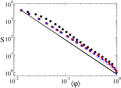
In Fig. 3 we plot $\langle\varphi\rangle$ vs $S$ obtained from computational simulations on a fully-connected system (empty circles) and on a 2D system for $v=0.1$ and different densities, and compare with the behavior predicted by Eq. (1i) (solid line). At $t=0$ ($S=N$) the expression from Eq. (1i) works very well because all velocities are actually randomly distributed, and thus the occupation number distribution is uniform ($n_{k}=1$ for all $k=1,..,N$). Then, as groups of particles start to have the same direction the $n_{k}$ distribution deviates from uniform, and thus the assumption $n_{k}(t)\simeq N/S(t)$ for all $k$ implemented above does not hold any more. However, for short times –or large values of $S$– the uniform approximation still works quite well, and the relation between $\varphi$ and $S$ for 2D systems is well described by Eq. (1i), as we can see in Fig. 3.

Figure 3: Average number of different directions $S$ vs average order parameter $\langle\varphi\rangle$ for a system of $N=4000$ particles, speed $v=0.1$, and densities $\rho=0.06$ (filled circles), $5$ (squares) and $50$ (triangles). Empty circles correspond to numerical results on a fully-connected system, while the solid line is the analytical estimation from Eq. (1i).

Combining Eqs. (1c) and (1i) we arrive to the following approximate expression for the time dependence of $\langle\varphi\rangle$

$$\left<\varphi\right>\simeq\frac{\sqrt{\pi}}{2}\left(\frac{1+t/2}{N}\right)^{1/2},$$ (1j)

indicated by a solid line in Fig. 1. Even though there are discrepancies between the numerics and the analytical expression Eq. (1j) for $t>1$, the algebraic increase $\left<\varphi\right>\sim\sqrt{t}/N$ for intermediate times (dashed line) predicted by Eq. (1j) seems to hold quite well for both particle densities. In Fig. 3 we can see that for a fixed value of $S$, 2D simulations (filled symbols) show more orientational order than the corresponding MF simulation (empty circles), as $\langle\varphi\rangle$ is larger in the former case. This is a consequence of the fact that in 2D the different directions of particles at a given time are not uniformly distributed in the $(-\pi,\pi]$ interval. Instead, longer lasting directions tend to be similar. This happens because orthogonal directions quickly tend to annihilate each other, given that interactions (and alignments) are more frequent between particles with high relative cross section. This can be seen in the $time=6800$ frame of Fig. 7 where the two largest clusters move almost parallel to each other.

4 Consensus times

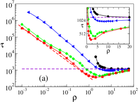
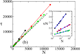
A magnitude of interest in models that exhibit a complete order is the time to reach the final ordered state or consensus time. In Fig. 4(a) we plot the mean consensus time $\tau$ over many realizations as a function of the particle density $\rho$, for a system of $N=600$ particles and different speeds. We need to mention that there was a very small fraction of realizations that did not reach consensus, specially at low densities. Those realizations were not considered in the calculation of $\tau$. In the static case scenario $v=0$ (circles) $\tau$ decreases with $\rho$ and approaches the MF value ($\tau_{\mbox{\tiny MF}}\simeq 2N=1200$) for large $N$ [8, 9] (horizontal dashed line). As discussed in section 3, the MF limiting case is obtained when $L\leq\sqrt{2}$ and thus each particle falls in the interaction range of any other particle. Therefore, for $N=600$ this happens when $\rho$ overcomes the value $N/2=300$. However, already for $\rho\simeq 50$ is $\tau\simeq\tau_{\mbox{\tiny MF}}$ and the system behaves as in MF. In Fig. 4(b) we show the dependence of $\tau$ with the number of particles for $v=0$ and different densities. For high densities, $\tau$ approaches the MF linear behavior $\tau_{\mbox{\tiny MF}}\simeq 2N$ (dashed line), but for low densities there are logarithmic deviations consistent with the 2D behavior $\tau\sim N\ln N$ [4, 5]. This crossover between 2D and MF can be better seen in the inset of Fig. 4(b), where we show $\tau/N$ vs $N$ on a log-linear scale to capture logarithmic corrections. We observe that data points fall on a straight line with density dependent $y$-coordinate $A(\rho)$ and slope $B(\rho)$. As $\rho$ increases, $B$ goes to zero and $A$ approaches $2.0$, recovering the MF behavior.

Figure 4: (a) Mean consensus time $\tau$ vs particle density $\rho$ for a system of $N=600$ particles and speeds $v=0$ (circles), $v=0.1$ (triangles), $v=5$ (diamonds) and $v=20$ (squares). The horizontal dashed line denotes the mean field consensus time $\tau_{\mbox{\tiny MF}}\simeq 2N=1200$, while the upper dashed line is the approximation from Eq. (1k). Inset: Same data on a linear-log scale showing the non-monotonic behavior regime. (b) $\tau$ vs $N$ for $v=0$ and densities $\rho=5$ (circles), $\rho=10$ (squares) and $\rho=21$ (diamonds). The dashed line is the expression $\tau=2N$. Inset: $\tau/N$ vs $N$ on a log-linear scale. Solid lines are the best linear fits $A(\rho)+B(\rho)\ln N$, with coefficients $A=1.285,1.668$ and $1.817$ and slopes $B=0.170,0.069$ and $0.032$ for densities $\rho=5,10$ and $21$, respectively.

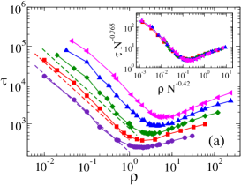
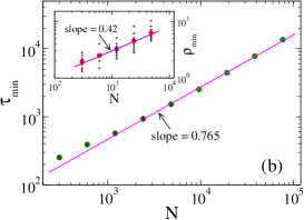
The dynamic case scenario $v>0$ is different from the static case $v=0$, as $\tau$ exhibits a non-monotonic behavior with $\rho$. The mean consensus time $\tau$ is much larger than $\tau_{\mbox{\tiny MF}}$ for low densities, but it decays to values smaller than $\tau_{\mbox{\tiny MF}}$ as $\rho$ increases and, after reaching a minimum value $\tau_{\mbox{\tiny min}}$, increases and saturates at the MF value. As expected, $\tau$ becomes independent of $v$ at high densities. The behavior of $\tau$ with the system size $N$ also shows interesting properties, as we see in Fig. 5(a) where we plot $\tau$ vs $\rho$ for a fixed speed $v=20$ and several values of $N$. The shape of all curves are non-monotonic, and the location of the minimum $\rho_{\mbox{\tiny min}}$ and its value $\tau_{\mbox{\tiny min}}$ increase with $N$. When the data corresponding to each size $N$ is shifted by the factors $N^{0.42}$ and $N^{0.765}$ on the $x$ and $y$ axis, respectively, all curves collapse into a single curve [see inset of Fig. 5(a)]. To obtain these scaling exponents we first selected a set of data points $(\rho_{\mbox{\tiny min}},\tau_{\mbox{\tiny min}})$ around the minimum of each curve, over an interval of $\rho$ where the curve $\tau(\rho)$ is approximately flat. The sets $(\tau_{\mbox{\tiny min}},N)$ and $(\rho_{\mbox{\tiny min}},N)$ which consisted on $43$ points each are plotted by dots in Fig. 5(b) and its inset, respectively, while circles correspond to average values for each $N$. By doing a linear regression analysis on a double logarithmic scale, $\ln(\rho_{\mbox{\tiny min}})=\alpha+\beta\ln(N)$, we obtained the estimators $\hat{\beta}=0.42$ and $\hat{\alpha}=-1.83$ that provide the best fit to the $(\rho_{\mbox{\tiny min}},N)$ data, and their associated error bars given by the $95\%$ confidence intervals $\beta=0.42\pm 0.09$ and $\alpha=-1.83\pm 0.64$, respectively. Then, we used the power-law best fit $\rho_{\mbox{\tiny min}}\simeq 0.16\,N^{0.42}$ to estimate $\rho_{\mbox{\tiny min}}$ for larger values of $N$ (up to $N=76800$) and calculated $\tau_{\mbox{\tiny min}}$ for those estimated minima. The results are plotted in Fig. 5(b) where we observe that $\tau_{\mbox{\tiny min}}$ follows an asymptotic power law in the interval $2400\lesssim N\lesssim 76800$, with an exponent $\gamma=0.765\pm 0.018$ (error bars were estimated using $25$ data points for $N=2400,4800,9600,19200,38400$ and $76800$). We note that the scaling $\tau_{\mbox{\tiny min}}\sim N^{0.765}$ is consistent with a consensus that is reached faster than in MF, where $\tau$ grows linearly with $N$.

Figure 5: (a) $\tau$ vs $\rho$ for speed $v=20$ and system sizes $N=300$ (circles), $600$ (squares), $1200$ (diamonds), $2400$ (up triangles) and $4800$ (left triangles). Dashed lines are the analytic approximation $2N/\pi\rho$ at low densities [Eq. (1k)], for $N=1200$, $600$ and $300$ (from top to bottom). Inset: Rescaled $\tau$ vs rescaled $\rho$ showing the collapse of the curves. (b) Auxiliary plots showing the regression lines with the exponents $\gamma=0.765\pm 0.018$ and $\beta=0.42\pm 0.09$ used in the inset of panel (a). Dots in the main plot and the inset correspond to the set of points $(\rho_{\mbox{\tiny min}},\tau_{\mbox{\tiny min}})$ around the minima of the $\tau$ vs $\rho$ curves of panel (a), while circles represent respective average values for each $N$. Main: Minimum mean consensus time $\tau_{\mbox{\tiny min}}$ vs $N$. The straight line is the power-law fitting function $\tau_{\mbox{\tiny min}}=2.378\,N^{0.765}$ for the range $2400\leq N\leq 76800$. Inset: Density at the minimum value of $\tau$, $\rho_{\mbox{\tiny min}}$, vs $N$. The straight line is the best fit $\rho_{\mbox{\tiny min}}=0.16\,N^{0.42}$ to the data.

The peculiar shape of $\tau$ vs $\rho$ is a consequence of the non-trivial interplay between particles’ speed and the propagation of directions over the space. We understand that the approach to consensus depends on the relation between the time scales associated to these two processes –convection and diffusion–, which vary with $\rho$ and $v$. Below we explore in more detail the origin of the non-monotonic behavior of $\tau$ with $\rho$. We first provide some scaling arguments that explain the behavior of $\tau$ in the limit of small densities and large speeds, and then study the clustering dynamics at intermediate and high densities.

4.1 Limit of small densities and high speeds

Let us consider the case where particles move fast, and so they travel such a long distance in each time step that their distribution remains nearly uniform over the box. This is so because the backward update [38] used in simulations involves two consecutive events: each particle first aligns its direction with a neighboring particle and then moves a distance $v$ with the old direction. As a consequence, for large speeds ($v\gtrsim L$) aligned particles could be at any distance from each other, leading to a quite uniform spatial pattern. Therefore, we can assume that the system remains well mixed at high speeds and thus interactions are as in MF. Then, at each time step, direction updates take place only among those particles that have at least one neighboring particle inside their interaction range. For each particle this happens with probability $p=1-(1-\pi\rho/N)^{N-1}\simeq\pi\rho$ for $\pi\rho\leq 1\ll N$, assuming that particles are uniformly distributed. The fact that particles not always update their directions at every time step introduces a time delay in the alignment dynamics, which rescales the MF consensus time $\tau_{\mbox{\tiny MF}}\simeq 2N$ by a factor of $1/p$ (the mean number of attempts between interactions). Therefore, we arrive to

$$\tau\simeq\frac{2N}{\pi\rho}~{}~{}~{}\mbox{for $\rho\leq\frac{1}{\pi}$}.$$ (1k)

We observe in Fig. 4(a) that the expression from Eq. (1k) (dashed line) gives a reasonable estimation of $\tau$ for high speed $v=20$ in the limit of low densities. The power-law decay $\tau\sim\rho^{-1}$ at low $\rho$ is also observed for speed $v=5$. Figure 5(a) shows how Eq. (1k) performs as the system size is varied (dashed lines). We see that for densities in the range $0.01<\rho<0.5$ the approximation is very good for $N=300$ (bottom line), but it becomes worst for larger system sizes $N=600$ (middle line) and $N=1200$ (top line). This is because by increasing $N$, while keeping $\rho$ and $v$ fixed, the box’s length $L=\sqrt{N/\rho}$ increases and thus the ratio $v/L$ eventually becomes small. Therefore, we expect that for large enough system sizes the well-mixed system assumption $v\gtrsim L$ does not hold any more, and thus the MF approximation is not longer valid. We also speculate that, for a fixed $N$, the agreement becomes better as $\rho$ decreases and gets far from the minimum, as we can see for the $N=600$ curve of Figs. 4(a) and 5(a). We observe as well that Eq. (1k) underestimates the numerical data at intermediate densities, where the formation of clusters plays an important role, as we show in the next subsection.

4.2 Clustering dynamics at intermediate and high densities

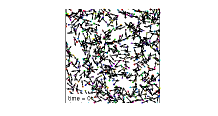
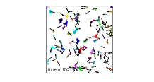
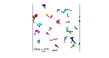
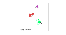
For intermediate densities, the consensus turns to be faster than in MF. This is consistent with the behavior of the number of different directions $S$ in Fig. 2. There we can see that $S$ decays as in MF ($S\sim N/t$) during an initial transient, but then it starts to decay faster (exponentially), leading to a consensus time that is smaller than $\tau_{\mbox{\tiny MF}}$. This effect is more pronounced for large speeds [see Fig. 2(b)]. As we explain below, the departure observed in $S$ from a power law to an exponential decay is caused by a dynamic reordering of the spatial pattern of interactions, from a well mixed system to structures localized in space. To explore this in more detail, we studied the time evolution of the mean number of neighbors $\left<k\right>$ (mean degree). Results are shown in Fig. 6 for $N=4000$ (the same as in Fig. 2), $v=20$ and various densities, where we observe that $\left<k\right>$ starts to increase very slowly from its initial value $\pi\rho$ –corresponding to a uniform distribution of particles– until it saturates for long times when the system reaches consensus. This increase in the number of neighbors suggests that particles aggregate into spatial clusters. Indeed, when two particles are less than a distance $R=1$ apart they can align their directions and then move together until one of them changes direction by interacting with a third particle. Thus, one can see that alignment implies the “sticking” of nearby particles, forming large sets of particles that move together in the same direction. These structures can be seen in Fig. 7 for a system of $N=600$ particles, with $v=0.1$ and $\rho=0.1$. The panels represent snapshots of the system at different times, showing the transition from a uniform distribution of particles moving in random directions at $t=0$ (a), to a spatial segregation into clusters of particles with the same direction at $t=150$ (b) and $t=470$ (c), and to a quasi-consensus state at $t=6800$. The segregation occurs for higher densities as well, but clusters may overlap when densities are very high.

Figure 6: Time evolution of the mean number of interacting neighbors $\left<k\right>$, for $N=4000$, speed $v=20$ and densities $\rho=0.06$ (circles), $\rho=2$ (squares), $\rho=5$ (diamonds) and $\rho=50$ (triangles).

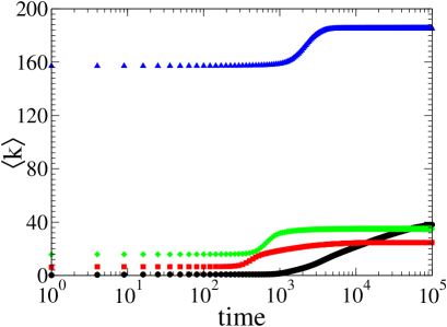
By comparing Fig. 2(b) with Fig. 6, we observe that the deviation of $S$ from the MF value starts approximately when $\langle k\rangle$ starts to be significantly larger than its initial value $\pi\rho$; for instance at time $t\simeq 400$ for $\rho=2$. This indicates that the formation of clusters speeds up the dynamics and the approach to consensus. It turns out that spatial segregation induces a drift in the transitions between directions, from directions followed by small clusters to directions of large clusters. In other words, large clusters are more likely to gain particles while small clusters tend to loose particles. This might seem obvious in a typical coarsening dynamics like the one in the Ising model, where smaller clusters tend to vanish and the average size of clusters increases with time. However, ordering in the original voter dynamics is quite different because same-state domains gain and loose particles at the same rate, independent on their size, and thus coarsening is only driven by fluctuations. This is due to the fact that all opinion states are equivalent in the VM on regular topologies [39] and, as consequence, the average fraction of particles in each state is conserved at all times. Therefore, the drift or net flow of particles between any two states is zero in the VM.

Figure 7: (Color online) Snapshots showing the configuration of the system at different times, composed by $N=600$ particles with a density $\rho=0.1$ and speed $v=0.1$. Particles are depicted by filled circles of radius $1.0$, thus interacting particles overlap in this scale. Arrows indicate the direction of motion of each cluster, shown in a particular color.

To study whether the transitions to a given direction $\alpha$ are correlated with the number of particles with direction $\alpha$ (mass $m_{\alpha}$), we define the drift from direction $\beta$ to direction $\alpha$ at time $t$ as

$$D(\beta\to\alpha,t)\equiv\sum_{i=1/\theta_{i}=\beta}^{N}p(\theta_{i}\to\alpha,t),$$ (1l)

where the sum is over all particles with direction $\theta_{i}=\beta$, and $p(\theta_{i}\to\alpha,t)$ is the probability that particle $i$ adopts the direction $\alpha$ at time $t$, calculated as the fraction of $i$’s neighbors with direction $\alpha$. Then, the net drift from small to large clusters is defined as

$$D(t)=\sum_{\alpha}\sum_{\beta}\mbox{sign}(m_{\alpha}-m_{\beta})\,D(\beta\to\alpha,t),$$ (1m)

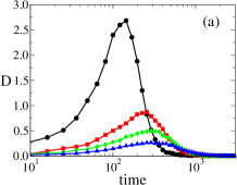
where sign($x$) is a function that takes the value $1$ ($-1$) for $x>0$ ($x<0$), and $0$ for $x=0$, thus it assigns a positive weight to drifts towards larger clusters, and a negative weight to drifts towards smaller clusters. Therefore, a positive (negative) value of $D$ means that, in average, the net drift in the system is from smaller (larger) to larger (smaller) clusters. In Fig. 8(a) we show the time evolution of $D$ averaged over $3\times 10^{4}$ realizations, on a system with $N=600$ particles moving at speed $v=5$ and for various densities. We observe that $D$ is larger than zero for all times, showing that there is a net drift from small to large clusters. This generates a positive feedback in which large clusters tend to increase their size while small clusters tend to shrink, and is in contrast with the MF behavior, where no direction has a prevalence on the others and thus $D=0$ at all times. Therefore, the presence of a positive drift breaks the symmetry of the system and speeds up the evolution towards consensus, as compared to MF. We can check that the MF limit is achieved as $\rho$ increases, where we see that $D$ decreases and is already very small for $\rho=31$.

Figure 8: Time evolution of four different magnitudes: (a) the net drift $D$ from small to large clusters, (b) the time derivative of the mean number of neighbors $\langle k\rangle$, (c) the ratio between the mean number of directions in MF ($S_{MF}$) and in 2D ($S$) as defined in Fig. 2, and (d) the covariance $\mbox{cov}(m,\langle k\rangle)$ between the size of a cluster and its mean degree. Simulations correspond to systems with $N=600$ particles, speed $v=5$ and densities $\rho=2$ (circles), $\rho=9$ (squares), $\rho=16$ (diamonds) and $\rho=31$ (triangles).

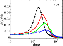
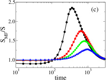
As we can see in Fig. 8(b), the shape of the time derivative of $\langle k\rangle$ agrees quite well with the shape of $D(t)$, showing a direct relationship between clustering and drift. Also, $D$ reaches a maximum when $S$ starts to deviate from the MF curve [see Fig. 8(c)], indicating that the drift accelerates the evolution towards consensus. Figure 8 shows only the case of $v=5$, but we found similar results for $v=0.1$ and $v=20$ as well. We speculate that the reason why larger clusters tend to increase their size more rapidly than smaller clusters is because particles that belong to larger clusters have, in average, a larger number of neighbors. And, it is known that in disordered topologies of interactions like complex networks, the weighted magnetization ($m=\sum_{i=1}^{N}S_{i}k_{i}/N$, with $S_{i}$ and $k_{i}$ the state and degree of node $i$, respectively) is conserved in the voter dynamics [39], rather than the state magnetization. This means that nodes are more likely to copy the opinion state of other nodes with large degrees, breaking the equivalence between states.

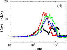
To check the relation between cluster size and mean degree we calculated the time evolution of the covariance $\mbox{cov}(m,\langle k\rangle)$ between the mass $m$ of a given cluster and the mean degree $\langle k\rangle$ of the particles that belong to that cluster, regardless whether the neighbors belong to the same or to a different cluster. The evolution of the covariance averaged over many realizations is shown in Fig. 8(d). We observe a positive covariance between $m$ and $\langle k\rangle$ which shows that, indeed, larger clusters have more neighbors, increasing their chances to gain more particles. A similar result was obtained in the SVM for which bigger clusters have larger mean degrees as well [40]. The fact that larger clusters tend to have a larger mean degree and grow faster, breaks the symmetry of the FVM.

5 Discussion and conclusions

We proposed and studied a flocking model in which self-propelled particles interact via a simple dynamics of velocity imitation. We studied the ordering dynamics of the system and its approach to the fully ordered state (consensus) $\langle\varphi\rangle=1$. We found that the dynamics is characterized by an algebraic increase with time ($\langle\varphi\rangle\sim t^{1/2}$) during an initial transient, and a final exponential approach to the ordered state. Interestingly, a similar ordering behavior is observed in the SVM model at zero noise, although the initial algebraic increase happens earlier, and thus the approach to order is much faster than in the FVM. We suspect that the scaling exponent $1/2$ found in the noiseless SVM might be related to the coarsening exponents found in the ordered phase of the SVM with noise [41, 42]. The ordering in the FVM is related to the decreasing number of different directions of motion in the system, which is well explained by the MF theory of the multi-state voter model during a first stage. On a second stage, and for high enough particle density $\rho$, the ordering dynamics is faster than in MF due to a break in the symmetry of directional states that speeds up the dynamics. As a consequence, the mean time to reach consensus $\tau$ is non-monotonic with $\rho$, that is, there is an optimal density for which the system reaches full order in the shortest time. The shape of the $\tau$ vs $\rho$ curve can be qualitatively explained in terms of three main mechanisms that act on different density scales. At low densities, the dynamics is limited by the sporadic encounters between particles that introduce a delay in the interactions and lead to large consensus times. At intermediate densities, the dynamics undergoes a breaking in the symmetry of transitions between directions, induced by the spatial segregation of particles into same-direction clusters. This symmetry breaking is enhanced by the motion of particles, generating a net mass drift from small to large clusters and accelerating the approach to consensus respect to the MF behavior. The sublinear scaling of the mean consensus time with $N$ at the minimum of the $\tau$ vs $\rho$ curve ($\tau_{\mbox{\tiny min}}\sim N^{0.765}$) is consistent with a consensus that is faster than in MF. Finally, at high densities the MF case of all-to-all interactions is recovered.

We explored a voter-like dynamics acting on self-propelled agents subject to metric interactions, which by definition occur when two particles are less than a predefined cutoff distance apart. This type of interactions was adopted for its simplicity. Nevertheless, it is known that some social living organisms, like birds or humans, may interact in a different way, for instance by considering the first $k$ closest neighbors regardless of the distance to them [43]. It would be worthwhile to study a system with voter-like interactions in this context. In particular, the density dependence of the dynamics could turn out to be very different with respect to the one found in this article, as it happens with the Vicsek model where the dynamics is essentially independent of the density in the case of non-metric interactions [44, 45]. Finally, a natural extension of the model would consist on the introduction of noise perturbing the direction of motion of particles as in the SVM. We plan to study this extended version of the FVM in a future work.

References

- [1] Castellano C, Fortunato S and Loreto V 2009 Rev. Mod. Phys. 81 591–646.
- [2] P. Clifford, and A. Sudbury, Biometrika 60, 581 (1973).
- [3] R. Holley and T. M. Liggett, Ann. Probab. 4, 195 (1975).
- [4] P. L. Krapivsky, Phys. Rev. A 45, 1067 (1992).
- [5] L. Frachebourg, and P. L. Krapivsky, Phys. Rev. E 53, 3009(R) (1996).
- [6] O. Al Hammal, H. Chaté, I. Dornic, and M. A. Muñoz, Phys. Rev. Lett. 94, 230601 (2005).
- [7] F. Vazquez and C. López, Phys. Rev. E 78, 061127 (2008).
- [8] M. Starnini, A. Baronchelli, and R. Pastor-Satorras, J. Stat. Mech. 2012, 10027 (2012).
- [9] W. Pickering and C. Lim, Phys. Rev. E 93, 032318 (2016).
- [10] Durrett R and Levin S A 1996 J. Theor. Biol. 179 119.
- [11] Chave J and Leigh E G 2002 Theor. Popul. Biol. 62 153.
- [12] Zillio T, Volkov I, Banavar J R, Hubbell S P and Maritan A 2005 Phys. Rev. Lett. 95.
-
[13]
Mobilia M 2003 Phys. Rev. Lett. 91
028701.
Mobilia M and Georgiev I T 2005 Phys. Rev. E 71 046102.
Mobilia M, Petersen A and Redner S 2007 J. Stat. Mech. P08029. -
[14]
Vazquez F, Krapivsky P L and Redner S 2003
J. Phys. A: Math. Gen. 36 L61.
Vazquez F and Redner S 2004 J. Phys. A: Math. Gen. 37 8479-94. - [15] Castelló X, Eguíluz V M and San Miguel M 2006 New J. Phys. 8 308; Stauffer D, Castelló X, Eguíluz V M and San Miguel M 2007 Physica A 374 835-42.
- [16] Antal T, Redner S and Sood V 2006 Phys. Rev. Lett. 96 188104.
- [17] Medeiros N G F, Silva A T C and Moreira F G B 2006 Phys. Rev. E 73 046120.
- [18] Dall’Asta L. and Castellano C., Europhys. Lett. 77 60005 (2007).
- [19] H.-U. Stark, C. J. Tessone, and F. Schweitzer, Physical Review Letters 101, 018701 (2008).
- [20] Naoki Masuda, N. Gibert, and S. Redner Phys. Rev. E 82, 010103 (2010).
- [21] Anthony Woolcock, Colm Connaughton, Yasmin Merali, and Federico Vazquez, Phys. Rev. E 96, 032313 (2017).
- [22] Sousa A. O., Yu-Song T. and Ausloos M., Eur. Phys. J. B, 66 (2008) 115.
- [23] Eur. Phys. Lett. 105, (2014) 30007.
- [24] Phys. Rev. E 95, 052308 (2017).
- [25] T. Vicsek, and A. Zafiris, Phys. Rep. 517, 71 (2012).
- [26] M. C. Marchetti, J. F. Joanny, S. Ramaswamy, T. B. Liverpool, J. Prost, Madan Rao, and R. Aditi Simha, Rev. Mod. Phys, 85, 1143, (2013).
- [27] A. M. Menzel, Phys. Rep. 554, 1 (2015).
- [28] I. D. Couzin, C. C. Ioannou, G. Demirel, T. Gross, C. J. Torney, A. Hartnett, L. Conradt, S. a. Levin, and N. E. Leonard, Science 334, 1578 (2011).
- [29] C. Huepe, G. Zschaler, A.-L. Do, T. Gross, New J. Phys. 13, 073022 (2011).
- [30] Buhl J, Sumpter D J T, Couzin I D, Hale J J, Despland E, Miller E R and Simpson S J 2006 Science 312 1402–6.
- [31] R. Martínez-García, C. López, and F. Vazquez, Phys. Rev. E 91, 022117 (2015).
- [32] M. Aldana, V. Dossetti, C. Huepe, V.M. Kenkre and H. Larralde, Phys. Rev. Lett., 98, 095702 (2007).
- [33] T. Vicsek, A. Czirók, E. Ben-Jacob, I. Cohen, and O. Shochet, Phys. Rev. Lett. 75, 1226 (1995).
- [34] Yen-Liang Chou and Thomas Ihle, Phys. Rev. E 91, 022103 (2015).
- [35] P. Holme and M. E. J. Newman, Phys. Rev. E 74, 056108 (2006).
- [36] F. Vazquez, V. M. Eguíluz, and M. San Miguel, Phys. Rev. Lett. 100, 108702 (2008).
- [37] F. Vazquez, Opinion dynamics on coevolving networks. Dynamics On and Of Complex Networks, Volume 2, Modeling and Simulation in Science, Engineering and Technology, pages 89-107. Springer New York, (2013).
- [38] G. Baglietto, and E. V. Albano, Phys. Rev. E 80, 050103(R) (2009).
- [39] K. Suchecki, V. M. Eguíluz and M. San Miguel , Europhys. Lett. 69, 228 (2005).
- [40] G. Baglietto, E. V. Albano, and J. Candia, J. Stat, Phys. 153, 270 (2013).
- [41] H. Chaté, F. Ginelli, G. Grégoire, and F. Raynaud, Phys. Rev. E 77, 046113 (2008).
- [42] S. Dey, D. Das, and R. Rajesh, Phys. Rev. Lett. 108, 238001 (2012).
- [43] M. Ballerini, N. Cabibbo, R. Candelier, A. Cavagna, E. Cisbani, I. Giardina, V. Lecomte, A. Orlandi, G. Parisi, A. Procaccini, M. Viale, and V. Zdravkovic, PNAS 105, 1232 (2008).
- [44] F. Ginelli and H. Chaté, Phys. Rev. Lett. 105 168103 (2010).
- [45] A. Peshkov, S. Ngo, E. Bertin, H. Chaté, and F. Ginelli, Phys. Rev. Lett. 109, 098101 (2012).