Lorentz symmetry violating low energy dispersion relations from a dimension-five photon scalar mixing operator

Abstract

Dimension-5 photon ($\gamma$) scalar ($\phi$) interaction terms usually appear in the bosonic sector of unified theories of electromagnetism and gravity. In these theories the three propagation eigenstates are different from the three field eigenstates. Dispersion relation, in an external magnetic field shows, that for a non-zero energy ($\omega$) out of the three propagating eigenstate one has superluminal phase velocity $v_{p}$. During propagation, another eigenstate undergoes amplification or attenuation, showing signs of an unstable system. The remaining one maintains causality. In this work, using techniques from optics as well as gravity, we identify the energy ($\omega$) interval outside which $v_{p}\leq c$ for the field eigenstates $~{}|\gamma_{\parallel}>$ and $|\phi>$, and stability of the system is restored. The behavior of group velocity $v_{g}$, is also explored in the same context. We conclude by pointing out its possible astrophysical implications.

Scalar $\phi(x)$ photon $\gamma$ interaction through dimension five operator originates in many theories beyond the standard model of particle physics, usually in the unified theories of electromagnetism and gravity duff . The scalars involved can be moduli fields of string theory, Kaluza-Klein (KK) particles from extra dimension, scalar component of the gravitational multiplet in extended supergravity models etc., to name a few [Schmutzer -Fischbach ].
Usually these models predict optical activity where the vacuum is turned into a birefringent and dichroic oneraffelt . As a polarized light beam passes through such a medium, its plane of polarization gets rotated. This particular aspect has been explored and exploited extensively in the literature to explain and predict many interesting physical phenomena Jain .
In this work we point out other interesting aspects of such interactions encountered in the low energy sector of the theory, in a magnetized background of field strength $\cal{B}$. The theory under consideration has a tree-level interaction term $g_{\phi\gamma\gamma}\phi F_{\mu\nu}F^{\mu\nu}$, where $g_{\phi\gamma\gamma}$ is a dimensionful coupling constant between $\phi$ and Electro Magnetic (EM) field. This term is Lorentz Invariant (LI) and remains invariant under charge conjugation (C), parity transformation (P) and time reversal (T) symmetry transformations. Renormalizability of the theory is compromised because of the presence of dimensionful coupling constant $g_{\phi\gamma\gamma}$. However, in the presence of an external background magnetic field, all the good (both continuous and discrete (i.e. LI and CPT)) symmetries of the theory get compromised. Since theories violating CPT are known to violate Lorentz invariance greenberg hence causality; therefore, the explicit violation of both in a nontrivial background introduces modifications to the dispersion relations affecting phase velocity ($v_{p}$) and group velocity ($v_{g}$). The same also introduces presence of unstable modes in a certain energy ($\omega$) domain. Some of these issues are explored below.
The theory under consideration has three propagation eigenstates, a scalar $|\phi\rangle$ and two transversely polarized photons $|\gamma_{||,\perp}\rangle$. ​​ One of the eigenstate, $|\gamma_{||}\rangle$ has polarization vector parallel and the other one, $|\gamma_{\perp}\rangle$ has the same orthogonal to the background magnetic field $\cal{B}$.
We point out in this note the two interesting possibilities that may emerge from the solutions of the two eigenstates, $|\phi\rangle$ and $|\gamma_{\parallel}\rangle$, (i) their phase velocity may become superluminal, (ii) their respective amplitudes may undergo attenuation or amplification, provided their energies lie in a certain interval. Within this energy interval the amplitudes of $|\gamma_{\parallel}\rangle$ and $|\phi\rangle$ may get amplified or damped, thus they are non-propagating modes.
Naively, though this phenomena seem to get ameliorated, only at energy $\omega=\infty$, but through a careful analysis we show that there exists a finite energy interval outside which, the individual field states $|\gamma_{\parallel}\rangle$ and $|\phi\rangle$ are cured of this malady. In other words outside that interval, the solutions of the same are well behaved as far as their stability and the magnitudes of the phase velocities (i.e., $v_{p}$ for $|\phi\rangle$ and $|\gamma_{\parallel}\rangle$, both ) are concerned.
The same however can not be endorsed for the group velocity $v_{g}$ for these two states. The same (i.e., $v_{g}$) for $|\phi\rangle$ and $|\gamma_{\parallel}\rangle$ reach luminal limit at $\omega=\infty$ only.
We note in the passing that, the phase velocities of $|\phi\rangle\pm|\gamma_{\parallel}\rangle$ do exhibit velocity selection rules as had been discussed in shore .
The other eigenstate $|\gamma_{\perp}\rangle$, is free from any pathological problems. It posses a stable solution as well as causal group and phase velocities, i.e., $v_{g}\!=\!v_{p}\!=\!c,~{}\forall x,t\mbox{~{}and~{}}\omega$.
In this article we analyze the issues involved, from three different angles, (a) using differential geometric arguments involving the properties of a metric ($g^{\mu\nu}_{(eff)}(\omega)$ in our context ) related to the stability of a manifold, as used in the context of relativity, (b) analyzing the Dispersion Relations (DR), and (c) by explicit evaluation of the phase velocities ($v_{p}$) from the solutions of the eigenstates, $|\gamma_{||,\perp}\rangle$ and $|\phi\rangle$, using principles of optics born-wolf .
A critical analysis of the DR actually conforms with the findings, obtained from the stability analysis of the effective metric, $g^{\mu\nu}_{(eff)}(\omega)$. The interesting part however is, $v_{p}$ turns out to be complex exactly in the same energy domain, as is predicted from the stability analysis of $g^{\mu\nu}_{(eff)}(\omega)$ as well as the dispersion relations. This indicates the system to be in an unstable state in the relevant energy domain. A detailed further analysis reveals that, outside this energy range, some of the Lorentz Invariance Violating (LIV) pieces in the expression of $v_{p}$, cancel out giving a LI and causal result. We conclude by pointing out the possible implications of this result in astrophysical or cosmological contexts.

Equations of motion: The action for coupled scalar photon system, in four dimensional flat space, is given by:

$$\!\!\!\!\!\!S\!=\!\!\!\int\!\!\!d^{4}x\!\!\left[\frac{1}{2}\partial{{}_{\mu}}\phi\partial^{\mu}\phi\!-\!\frac{1}{4}g_{\phi\gamma\gamma}\phi F_{\mu\nu}F^{\mu\nu}\!-\!\frac{1}{4}F_{\mu\nu}F^{\mu\nu}\!\right].$$ (1)

The equations of motion can be obtained from eqn.[1] by employing the usual variational principles. However, in what follows, we would rewrite eqn.[1] by decomposing the EM field tensor $F_{\mu\nu}$ into two parts, a slowly varying Background Mean Field ${\bar{F}_{\mu\nu}}$, and an infinitesimal fluctuation $f_{\mu\nu}$ (i.e.,​​​ :​​​ $F_{\mu\nu}={\bar{F}_{\mu\nu}}+f_{\mu\nu}$), and then derive the equations of motion from the modified action. And without loss of generality, we would consider a local inertial frame, where, the only nonzero component of $\bar{F}^{\mu\nu}$, is $\bar{F}^{12}={\cal{B}}$. ​​Assuming the magnitude of the scalar field to be of the order of the fluctuating EM field $f_{\mu\nu}$, one can linearize the resulting equations. The resulting equations of motion for the EM and the scalar fields turn out to be,

$$\partial_{\mu}f^{\mu\nu}=-g_{\phi\gamma\gamma}\partial_{\mu}\phi\bar{F}^{\mu\nu},$$ (2)

$$\partial_{\mu}\partial^{\mu}\phi=-\frac{1}{2}g_{\phi\gamma\gamma}\bar{F}^{\mu\nu}f_{\mu\nu}.$$ (3)

Equation [2] describes the evolution of the two degrees of freedom associated with the gauge fields and eqn. [3] describes the same for the scalar field. Since eqn. [2] provides four equations for two degrees of freedom of the gauge fields, so one has to get rid of the extra relations by fixing a gauge and using the constraint equation.
However, there is another way, i.e., by working in terms of the field strength tensors and making use of the Bianchi identity. In this work we will follow the second method. We will start with the Bianchi identity $\partial_{\mu}f_{\nu\lambda}+\partial_{\nu}f_{\lambda\mu}+\partial_{\lambda}f_{\mu\nu}=0$ and multiply the same by $\bar{F}^{\nu\lambda}$; after this we operate $\partial^{\mu}$ on the resulting expression, to arrive at:

$$\partial_{\mu}\partial^{\mu}(f_{\lambda\rho}\bar{F}^{\lambda\rho})=-2\partial^{\lambda}\partial_{\mu}(f^{\mu\rho}\bar{F}_{\rho\lambda}).$$ (4)

Next we can multiply eqn.[2] by ${\bar{F}}_{\nu\lambda}$, and subsequently operate ${\partial}^{\lambda}$ on the same to obtain,

$$\partial^{\lambda}\partial_{\mu}(f^{\mu\nu}{\bar{F}}_{\nu\lambda})=-g_{\phi\gamma\gamma}\partial^{\lambda}\partial_{\mu}\phi{\bar{F}}^{\mu\nu}{\bar{F}}_{\nu\lambda}.$$

Now using the relation given by eqn.[4], on the last equation, we find the equation for the eigenstate $|\gamma_{||}\rangle$, given by:

$$\partial_{\mu}\partial^{\mu}\left(f_{\rho\sigma}\bar{F}^{\rho\sigma}/2\right)=g_{\phi\gamma\gamma}\partial^{\lambda}\partial_{\alpha}\phi(\bar{F}^{\alpha\nu}\bar{F}_{\nu\lambda}).$$ (5)

The equation for the eigenstate $|\gamma_{\perp}\rangle$, can be obtained by performing the same steps leading to eqn.[5], except the multiplication of eqn.[2] by the factor $\bar{F}_{\nu\lambda}$. In this step, instead of $\bar{F}_{\nu\lambda}$ we have to use the multiplicative factor $\tilde{\bar{F}}_{\nu\lambda}$. This would lead us to:

$$\partial_{\mu}\partial^{\mu}(f_{\nu\lambda}\tilde{\bar{F}}^{\nu\lambda}/2)=0,$$ (6)

It is easy to perform a consistency check on eqn.[6] using eqn.[5]. If we replace $\bar{F}_{\nu\lambda}$ by ${\tilde{\bar{F}}}_{\nu\lambda}$ in eqn.[5] then we immediately recover eqn.[6], because the right hand side of eqn.[5] vanishes; since $\bar{F}^{\alpha\nu}\tilde{\bar{F}}_{\nu\lambda}=0$, because of our assumption that, for the background EM field, only $\bar{F}^{12}\neq 0$. Hence eqn.[6] is consistent.
Now we introduce the new set of variables, $\psi\!=\!\frac{f_{\nu\lambda}\bar{F}^{\nu\lambda}}{2}$ and $\tilde{\psi}\!=\!\frac{f_{\nu\lambda}\tilde{\bar{F}}^{\nu\lambda}}{2}$, and use them in eqns.[5,6], and subsequently go to momentum space, to obtain the dispersion relations. Those are given by:

$$k^{2}\psi-g_{\phi\gamma\gamma}\left(k_{\alpha}\bar{F}^{\alpha\nu}\bar{F}_{\nu\lambda}k^{\lambda}\right)\phi=0,~{}~{}k^{2}\tilde{\psi}=0~{}~{}\mbox{~{}and~{}}~{}~{}k^{2}\phi-g_{\phi\gamma\gamma}\psi=0.$$ (7)

Since we have assumed, that only $\bar{F}^{12}\!\!=\!\!{\cal{B}}\!\!=\!\!\tilde{\bar{F}}^{03}\!\!\neq\!\!0$, then it follows from there, that:​​​ $\left(\bar{F}^{\mu\nu}\bar{F}_{\mu\nu}\right)\!\!=\!\!2{\cal{B}}^{2}$ and $\left(k_{\alpha}\bar{F}^{\alpha\nu}\bar{F}_{\nu\lambda}k^{\lambda}\!\right)\!\!=\!\!k^{2}_{\perp}\!{\cal{B}}^{2}$. Furthermore, if the angle between ${\cal{B}}$ and $\vec{K}$ is $\Theta$, then the component of ${\vec{K}}$ normal to $\cal{B}$ is: $\vec{k}_{\perp}=\vec{K}\rm{sin}~{}\Theta$. Hence, using the same one can denote:

$$k^{2}_{\perp}{\cal{B}}^{2}=K^{2}sin^{2}\Theta{\cal{B}}^{2}\simeq\left(\omega{\cal{B}}sin\Theta\right)^{2}.$$ (8)

While rewriting the eqn. [8], it was assumed that, $\omega\simeq K$ to zeroth order in the coupling constant $g_{\phi\gamma\gamma}$. From now on, for the sake of brevity, we may denote ${\cal{B}}sin\Theta={\cal{B}}_{T}$, at times.
In order to make the mass dimension of $\psi,{\tilde{\psi}}$ and $\phi$ same, we can multiply eqn.[7] by $\omega{\cal{B}}sin\Theta$ and redefine $\Phi=\omega{\cal{B}}sin\Theta\phi$. Upon doing the same, the coupled dispersion relations can be cast as a matrix equation:

$$\left[\begin{matrix}&k^{2}&0&0\cr&0&k^{2}&-g_{\phi\gamma\gamma}\left(\omega{\cal{B}}_{T}\right)\cr&0&-g_{\phi\gamma\gamma}\left(\omega{\cal{B}}_{T}\right)&k^{2}\end{matrix}\right]\!\!\!\left[\begin{matrix}{\tilde{\psi}}\cr\psi\cr\Phi\end{matrix}\right]=0.$$ (9)

The real symmetric matrix, in eqn.[9], can be diagonalized by a orthogonal rotation through angle $\theta$, in the $\psi$-$\Phi$ plane.

Propagation Eigenstates: We already have explained, that, ${\tilde{\psi}}$ and $\psi$ have their respective polarization vectors $\perp$ and $\parallel$ to ${\cal{B}}$. The off-diagonal elements in eqn. [9] make $\psi$ and $\Phi$ to mix during their space-time evolution; while $\tilde{\psi}$ remains unaffected. Next we diagonalize eqn.[9], by the orthogonal transformation discussed before, and express the same as:

$$\!\!\!\!\left(\begin{matrix}&\!\!\!k^{2}&\!\!\!0&\!\!\!0\cr&\!\!\!\!0&\!\!k^{2}-g_{\phi\gamma\gamma}{\cal{B}}_{T}\omega&\!\!\!0\cr&\!\!\!\!0&\!\!\!0&\!\!\!\!\!\!\!\!\!\!k^{2}+g_{\phi\gamma\gamma}{\cal{B}}_{T}\omega\end{matrix}\right)\!\!\!\left(\begin{matrix}\tilde{\psi}\cr\frac{\Phi+\psi}{\sqrt{2}}\cr\frac{\Phi-\psi}{\sqrt{2}}\end{matrix}\right)\!\!\!=\!0.$$ (10)

It is easy to see from eqn. [10] that, the propagating eigenstates $\tilde{\psi}$, $\frac{\Phi+\psi}{\sqrt{2}}$ and $\frac{\Phi-\psi}{\sqrt{2}}$ satisfy the following dispersion relations,

$$\omega = K$$ (11)

$$\omega_{+} = \pm\sqrt{K^{2}+g_{\phi\gamma\gamma}{\cal{B}}_{T}\omega}$$ (12)

$$\omega_{-} = \pm\sqrt{K^{2}-g_{\phi\gamma\gamma}{\cal{B}}_{T}\omega}.$$ (13)

We point out that the dispersion relations obtained from eqns.[9,10] are identical to those obtained in [Iacopini ; Miani ; Ganguly3 ], provided appropriate limits are taken.
Upon dividing eqns.[12,13] by $K$, we arrive at the expressions for the phase velocities, $v^{\pm}_{p}={\sqrt{1\pm g_{\phi\gamma\gamma}\cal{B}_{T}/\omega}}$, corresponding to the propagation eigenstates, $[\frac{\Phi\pm\Psi}{\sqrt{2}}]$. It is easy to verify that, for $g_{\phi\gamma\gamma}\cal{B}_{T}>\omega$, the magnitude of $v^{+}_{p}>1$ that is, phase velocity of the eigenstate $[\frac{\Phi+\Psi}{\sqrt{2}}]$ propagates with superluminal speed, and $v^{-}_{p}$ is complex so the amplitude of the corresponding eigenstate $[\frac{\Phi+\Psi}{\sqrt{2}}]$ would be attenuated or damped, as was mentioned in the beginning.

Effective metric: To understand more about the Lorentz Invariance Violating (LIV) dispersion relation in the magnetized vacuum for the mixed propagation eigenstate $\left[\frac{\Psi+\Phi}{\sqrt{2}}\right]$, we note that the dispersion relation for the same can be written as $g^{\mu\nu}_{(eff)}(\omega)k_{\mu}k_{\nu}=0$, where, $g^{\mu\nu}_{(eff)}(\omega)=diag\left(\left[1-\frac{g_{\phi\gamma\gamma}{\cal{B}}sin\Theta}{\omega}\right],-1,-1,-1\right)$ and $k_{\mu}$ is the usual wave 4-vector. The form of the effective metric given above is similar to the ones discussed in the context of Doubly Special Relativity (DSR) kimberly . We clarify at the outset that the same has been obtained, here, by demanding that the dispersion relation can be written as a quadratic of $k_{\mu}$’s, like the same for mass-less particles. One may interpret this effective metric as, the metric of the underlying spacetime over which $\left[\frac{\Psi+\Phi}{\sqrt{2}}\right]$ is propagating. The inverse of the same is $g_{\mu\nu(eff)}(\omega)$ is given by, $g_{\mu\nu(eff)}(\omega)=diag\left(\frac{1}{\left[1-\frac{g_{\phi\gamma\gamma}{\cal{B}}sin\Theta}{\omega}\right]},-1,-1,-1\right)$. Next we would perform stability analysis of the system using this metric.

Stability Analysis Using $\mathbf{g_{\mu\nu(eff)}(\omega)}$: It has been pointed out in LL , that, for a space-time to be stable, the determinant of it’s metric must be negative, else the system is unstable and would decay to a stable ground state. The purpose of writing the effective metric was to find out if there exists a bound or interval over which determinant of the same is negative indicating possibility of attenuation or growth of the amplitudes of the eigenmodes.
If we take a critical look at $g_{\mu\nu(eff)}(\omega)$, it is clearly seen that unless $\omega>g_{\phi\gamma\gamma}{\cal{B}}sin\Theta=\omega_{c}$ the value of $Det|g_{\mu\nu(eff)}(\omega)|>0$, hence there would be growth (instability) or damping (attenuation) in the system. Now if we go back to eqn. [12] one can verify that, the same can be recast in the following form, $\left(\omega-\frac{g_{\phi\gamma\gamma}{\cal{B}}sin\Theta}{2}\right)^{2}-\left(\frac{g_{\phi\gamma\gamma}{\cal{B}}sin\Theta}{2}\right)^{2}=K^{2}$. Accordingly, for $\omega<\omega_{c}$, wave vector $K$ becomes imaginary, signaling attenuation or growth of amplitude. Therefore, we are tempted to conclude that the deductions of LL , holds even for the effective metric $g_{\mu\nu(eff)}(\omega)$.

Causal Stability: It has been pointed out in hawking ; astro-2 ; novello that the stability of causal manifolds are governed by two conditions, (a) the underlying metric has to be Lorenzian and (b) there should exist a scalar time-like function $T(x)$, i.e. continuous and infinitely differentiable every where on the manifold; and covariant derivative of $T(x)$ i.e., $D_{\mu}T(x)\neq 0$, and $g^{\mu\nu}_{(eff)}(\omega)D_{\mu}T(x)D_{\nu}T(x)>0$ Klinkhammer ; klinkhammer2 . In our case both the conditions are satisfied, provided, we take $T(x)=t$ as the time coordinate (i.e., illustrating the absence of closed time like or space like curves).

Inhomogeneous Wave Equations: It is possible to get the solutions for the propagating eigenstates $\tilde{\psi}$, $\frac{\Phi+\psi}{\sqrt{2}}$ and $\frac{\Phi-\psi}{\sqrt{2}}$ from the dispersion relations given by eqns.[11,12,13], that follows from eqn.[10].
Sometimes, presenting results in its full generality, becomes a fruitful and instructive exercise in many areas of exact science. It helps in pointing out potential sources of new scientific features. Keeping this philosophy in mind we express the solutions of the coupled set of equations, as an explicit function of the rotation angle $\theta$, in the $\psi-\Phi$ plane. They have the following form,

$$\left(\begin{matrix}\tilde{\psi}\cr cos\theta~{}\psi+sin\theta~{}\Phi\cr-sin\theta~{}\psi+cos\theta~{}\Phi\end{matrix}\right)=\left(\begin{matrix}A_{0}e^{i\left(\omega t-k.x\right)}\cr A_{1}e^{i\left(\omega_{+}t-k.x\right)}\cr A_{2}e^{i\left(\omega_{-}t-k.x\right)}\end{matrix}\right)$$ (14)

It is not difficult to see, that for $\theta=\pi/4$, one recovers, back the expressions for propagating eigen states, $\frac{\Phi\pm\psi}{\sqrt{2}}$. We would like to mention here that, we would not consider, $\theta=\frac{\pi}{4}$, till we reach an appropriate point.
The constants, $A_{0},~{}A_{1}$  and $A_{2}$ appearing in eqn.[14], are to be derived from the boundary conditions one imposes on the dynamical degrees of freedom. The solutions for the dynamical variables, from eqn.[14], turn out to be,

$$\!\!\!\tilde{\psi}(t,x)\!=\!\!A_{0}e^{i\left(\omega t-k.x\right)},\psi(t,x)\!\!=\!\!\left[A_{1}cos\theta e^{i\omega_{+}t}\!-\!\!A_{2}sin\theta e^{i\omega_{-}t}\right]\!e^{-ikx}\mbox{~{}and~{}}\Phi(t,x)\!=\!\!\left[A_{1}sin\theta e^{i\omega_{+}t}\!+\!A_{2}cos\theta e^{i\omega_{-}t}\!\right]\!e^{-ik.x}\!.$$ (15)

In the following we consider the boundary conditions, $\Phi(0,0)=0$ and $\psi(0,0)=1$. With these boundary conditions, we have, $\frac{A_{2}}{sin\theta}=-1$ and the solution for $\psi$ turns out to be,

$$\!\!\!\!\psi(t,x)\!\!=\!\left[cos^{2}\theta\,\,e^{i\left(\omega_{+}t-k.x\right)}\!\!+\!\!sin^{2}\theta\,\,e^{i\left(\omega_{-}t-k.x\right)}\right].$$ (16)

Defining, $a^{2}_{x}(t)=\left({\rm{\cal{R}}}e\left[\psi(t,0)\right]\right)^{2}+\left(\rm{\cal{I}}m\left[\psi(t,0)\right]\right)^{2}$, we get the following form for $\psi\left(t,x\right)$,

$$\!\!\!\psi(t,x)\!\!=\!\!a_{x}(t)e^{\!i\!\left(tan^{-1}\!\left[\frac{cos^{2}\theta sin\omega_{+}t+sin^{2}\theta\,sin\omega_{-}t}{cos^{2}\theta\,cos\omega_{+}t+sin^{2}\theta\,cos\omega_{-}t}\right]-kx\!\!\right)}$$ (17)

A wave equation of this type is usually called inhomogeneous wave equation born-wolf . The phase velocity for such a system, where the solution is represented by, $a(t)e^{i(\varphi(t)-k.x)}$ is defined by, $v_{p}=\frac{1}{K}\frac{\partial\varphi(t)}{\partial t}$.
In more complicated physical situations, when medium effects, polarization effects due to strong external fields etc., are taken into account, the angle $\theta$ would depend on those parameters. Hence $\varphi(t)$ may become a complicated function of time. As a result, the phase velocity, $v_{p}$ may become a function of time with varied physical implications.
However, for the simple case in hand, substituting $\theta=\frac{\pi}{4}$ in eqn. [17], followed by some algebra, it is easy to demonstrate that, $\varphi(t)=\frac{\left(\omega_{+}+\omega_{-}\right)t}{2}$. Now using the same in the expression for phase velocity $v_{p}$ yields,

$$v_{p}=\left(\frac{\omega_{+}+\omega_{-}}{2K}\right)$$ (18)

Using eqns. [12] and [13] in eqn.[18] and considering the dispersion relation to zeroth order in $g_{\phi\gamma\gamma}$, i.e., $\omega\simeq K$, we obtain,

$$v_{p}\!=\!\frac{1}{2}\!\!\left[\!\sqrt{\!\!\left(\!\!1\!\!-\frac{g_{\phi\gamma\gamma}\cal{B}_{T}}{\omega}\!\!\right)}\!+\!\sqrt{\!\!\left(\!\!1\!\!+\!\frac{g_{\phi\gamma\gamma}\cal{B}_{T}}{\omega}\right)}\right]$$ (19)

The expression for phase velocity, as given by eqn. [19], provides an interesting limit for $\omega$; in order to have a real phase velocity, one must have $\omega\geq g_{\phi\gamma\gamma}\cal{B}_{T}$. So in principle one can define an expansion parameter $\delta=\frac{g_{\phi\gamma\gamma}\cal{B}_{T}}{\omega}$, and perform an all order expansion of $\left(1\pm\frac{g_{\phi\gamma\gamma}\cal{B}_{T}}{\omega}\right)^{1/2}$, in powers of $\delta$, for $\delta<1$, and be convinced that the magnitude of $v_{p}$ stays less than $c$, i.e. phase velocity is causal.

Group velocity: Group velocity for the situation under consideration is given by, $v_{g}=|\frac{\partial\dot{\varphi}}{\partial K}|$. Using the expression for $\dot{\varphi}$, in the last relation, we obtain the expression for group velocity in terms of $\delta$,

$$\hskip-28.45274ptv_{g}\!=\!\frac{1}{2}\!\left[\!\frac{1-\frac{\delta}{2}}{\sqrt{1-\delta}}+\frac{1+\frac{\delta}{2}}{\sqrt{1+\delta}}\!\right]\!,$$ (20)

Expanding the right-hand side of eqn.(20) in powers of $\delta$ (assuming $\delta<1$), one finds that $v_{g}>1$, even when, $0<\delta<1$. Of course the problem of having complex $v_{g}$ is avoided by considering $\delta<1$, however the issue of superluminality remains. We believe, that this is an artifact of the special background that violates Lorentz and CPT invariance. The presence of this special background may be responsible for making $v_{g}$ of the $|\gamma_{\parallel}\rangle$ state superluminal.

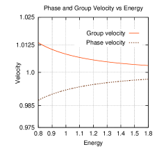
Figure 1: Plot of Velocity vs Energy. Energy is plotted in units of $10^{-15}$ GeV. The other parameters being $g_{\phi\gamma\gamma}=(10^{-11}\rm{GeV})^{-1}$ and ${\cal B}$=$10^{9}$ Gauss.

In Fig.[1], we have plotted $v_{g}$ and $v_{p}$, for various values of $\omega$. As can be seen from the plots, that as energy, $\omega\to\infty$ the group (phase) velocity, $v_{g(p)}\to 1$.
The solution for $|\phi\rangle$, is similar to $|\gamma_{\parallel}\rangle$ modulo a constant phase factor. It seems that, for $\omega<\omega_{c}$, there is energy exchange between these two modes. A detailed understanding of the physics of energy transfer as well as how the system behaves once the back-reaction of the propagating modes on the background is taken into account, following [cooper and boyanovsky ], seems to be an important issue. However addressing the same are beyond the aim and the scope of the current article and would not be dealt with any further here.

Signature: In astrophysical situations synchrotron or curvature radiation is the most common process of non-thermal emission. As is well known, from Ginzburg , that such radiations are always polarized along and orthogonal to the ${\mathcal{B}}-V$ plane. Where $V$ is the instantaneous velocity vector of the radiating charged particle. The synchrotron amplitudes of the electromagnetic radiation for these two polarized states are given by,

$$A_{\perp}=\frac{\sqrt{3}\gamma^{2}_{f}\theta_{e}}{\omega_{r}}\sqrt{1+\gamma^{2}_{f}\theta^{2}_{e}}K_{1/3}\left(\frac{\omega}{2\omega_{r}}\right),$$

$$\vspace{-2em}A_{\parallel}=i\frac{\sqrt{3}\gamma_{f}}{\omega_{r}}\left(1+\gamma^{2}_{f}\theta^{2}_{e}\right)K_{2/3}\left(\frac{\omega}{2\omega_{r}}\right).$$ (21)

In eqns. [21], $\gamma_{f}$ is the Lorentz factor, $\omega_{r}=\frac{3\gamma^{3}_{f}}{\rho}$ is the cutoff frequency and $\rho$ is the radius of curvature of the trajectory of the radiating particle. Lastly $\theta_{c}=\frac{1}{\gamma_{f}}$ is the opening angle of the radiating cone.
Since for $\omega<\omega_{c}$, the only evolving polarized state is $|\gamma_{\perp}\rangle$ when dimension-5, $\phi F_{\mu\nu}F^{\mu\nu}$ interaction is present, therefore, to a far away observer, the synchrotron radiation would appear to be linearly polarized.
So, the differential intensity spectrum per unit energy, per unit solid angle at the source for the $|\gamma_{\perp}\rangle$ state, following eqn.[21], is given by: $\frac{d^{2}I}{d\omega d\Omega}=\frac{(e\omega)^{2}}{4\pi^{2}}\left(|A_{\perp}|^{2}\right)$. Further more, if all the astrophysical absorption mechanisms are negligible, then the magnitude of $\frac{d^{2}I}{d\omega d\Omega}$, at the source, as well as, at the observation point would remain the same. Therefore, the differential intensity spectrum for two different energies $(\omega_{1},\omega_{2}<\omega_{c})$, would be related to the respective energies, $\omega_{1}$ and $\omega_{2}$ by,

$$\!\!\!\!\!\!\!\!\!\frac{\frac{d^{2}I(\omega_{1})}{d\omega_{1}d\Omega}}{\frac{d^{2}I(\omega_{2})}{d\omega_{2}d\Omega}}\!\!=\!\!\left[\frac{\omega_{1}K_{\frac{1}{3}}\!\!\left(\frac{\omega_{1}}{2\omega_{c}}\right)}{\omega_{2}K_{\frac{1}{3}}\!\!\left(\frac{\omega_{2}}{2\omega_{c}}\right)}\right]^{2}\!\!\!\!\!\rm{~{},implying,~{}~{}}\!\!\frac{\omega_{2}}{\omega_{1}}\!\!=\!\!\left[\frac{\frac{d^{2}I(\omega_{1})}{d\omega_{1}d\Omega}}{\frac{d^{2}I(\omega_{2})}{d\omega_{2}d\Omega}}\right]^{\frac{3}{4}}\!\!\!.$$ (22)

This is the intensity – energy relation. While deriving the same (i.e., eqn. [22]), we have used eqn.[21] and expanded $K_{1/3}(x)$ in decending powers of $x$.
Next we would like to relate this intensity – energy relation (eqn. [22]) with the rotation measure.
Since the intervening media between the source and the far-away observer is magnetized and composed of nonrelativistic, degenerate electrons; the Plane Of Polarization (POP) of a polarized light (of energy $\omega$) passing through the same would undergo Faraday Rotation (FR), given by GKP ,

$$\varphi=\frac{\alpha\pi\left({\cal{B}}\cos{\Theta}\right)}{\omega^{2}m_{e}}nl+\zeta.$$ (23)

Here, $\zeta$ is the angle between POP and ${\hat{\cal B}}$ at source and $l$ is the length of the path travelled. Rest of the symbols in eqn. [23] have their usual meaning.
Since the net rotation measure ($\varphi-\zeta$) due to FR goes as $\frac{1}{\omega^{2}}$; therefore, for a multi-frequency plane polarized light beam, the ratio of the two rotation measures at two distinct energies ($\omega_{1}$ and $\omega_{2}$), will be given by the following relation,

$$\omega_{2}/\omega_{1}=\sqrt{\left(\varphi_{1}-\zeta\right)/\left(\varphi_{2}-\zeta\right)}~{}.$$ (24)

Eqn.[24] may henceforth be termed as Energy-Dependent-Rotation Measure (EDRM).
Now we can use eqns. [22] and [24], to arrive at a relation between the rotation measure and the differential intensity spectrum, for $\tilde{\psi}$ ( i.e., the solution for $|\gamma_{\perp}\rangle$ state), and the same is:

$$\frac{\left(\varphi_{1}-\zeta\right)}{\left(\varphi_{2}-\zeta\right)}=\left[\frac{d^{2}I(\omega_{1})}{d\omega_{1}d\Omega}\div\frac{d^{2}I(\omega_{2})}{d\omega_{2}d\Omega}\right]^{\frac{3}{2}}.$$ (25)

For magnetic field strength at source, ${\cal{B}}\sim 10^{9}$ Gauss, and $g_{\phi\gamma\gamma}\sim\left(10^{11}GeV\right)^{-1}$, we have $\omega_{c}\sim 10^{-5}eV$ which lies in the radio range.
So, the polarization versus (differential) intensity distribution pattern, for plane polarized light, in the energy range, $0<\omega<10^{-5}eV$, from distant astrophysical objects (with dominant synchrotron source), should behave according to eqns. [22] and [25].

Conversely, for $\omega$ above $\omega_{c}$, both, $\tilde{\psi}$ and $\psi$ would propagate in space-time. And $\psi$ would undergo amplitude modulation because of mixing with $\Phi$. Hence, the emerging light beam may bear some appropriate polarimetric mybook and dispersive signatures of $g_{\phi\gamma\gamma}\phi\bar{F}_{\mu\nu}F^{\mu\nu}$ interaction, when the Faraday and the mixing effects are considered together, provided, the same is realized in nature.
Similar signatures from different astrophysical radio sources were reported in cfj and TJ sometimes back. They may have some implications for the situation we have discussed in this note. However one should work with the new data sets before coming to a definite conclusion.

Acknowledgment: We would like to thank the referee for his constructive criticism and suggestions.

References

- (1) M. J. Duff, B. E. W. Nilsson and C. N. Pope, Phys. Rep. 130, 1, (1986).
- (2) E. Schmutzer, in Unified Field Theories of More Than 4 Dimensions, edited by E. Schmutzer and V. De Sabbata (World Scientific, Singapore, 1983), p. 81.
- (3) J. Scherk, in Supergravity, edited by P. van Nieuwenhuizen and D. Z. Freedman (North-Holland, Amsterdam, 1979), p. 43.
- (4) P. G. Bergmann, Int. J. Theor. Phys. 1, 25 (1968).
- (5) M. Gasperini, Gen. Relativ. Gravit. 16, 1031 (1984) .
- (6) P. G. Roll, R. Krotkov and R. H. Dicke, Ann. Phys. (N.Y.) 26, 442 (1964).
- (7) V. B. Braginsky and V. I. Panov, Zh. Eksp. Teor. Fiz. 61, 873 (1971) [Sov. Phys. JETP 34, 463 (1972)].
- (8) G. W. Gibbons and B. F. Whiting, Nature (London) 291, 636 (1981).
- (9) E. Fischbach, D. Sudarsky, A. Szafer, C. Talmadge and S. H. Aronson, Phys. Rev. Lett. 56, 3 (1986).
- (10) G. Raffelt and L. Stodolsky, Phys. Rev D37,1237 (1988).
- (11) A. K. Ganguly, P. Jain and S. Mandal, Phys.Rev. D79, 115014, (2009); N. Agarwal, P. Jain, D. W. McKay, J. P. Ralston, Phys.Rev. D78, 085028, (2008); S. Das, P. Jain, J. P. Ralston, R. Saha, JCAP 0506, 002 (2005).
- (12) O. W. Greenberg, Phys. Rev. Lett. 89,231602 (2002).
- (13) G. Shore, Nucl.Phys. B717, 86 (2005).
- (14) M. Born, & E Wolf, Principles of Optics,(1980) sixth edn. (Pergamon Press).
- (15) E. Iacopini and E. Zavattini, Phys. Lett. 85B, 151 (1979).
- (16) L. Maiani, R. Petronzio and E. Zavattini, Phys. Lett. B 175, 359 (1986)
- (17) L. Miani, R. Petronzio and E. Zavattini, Phys. Lett. B175 359 (1986). M. Gasperini, Phys. Rev. D36, 2318 (1987). A. K. Ganguly and R. Parthasarathy, Phys. Rev. D68, 106005 (2003).
- (18) D. Kimberly, J. Magueijo and J. Medeiros, Phys. Rev. D70, 084007 (2004).
- (19) L.D. Landau, E.M. Lifshitz (1975). The Classical Theory of Fields. Vol. 2 (4th ed.). ( Pergamon Press ); S. W. Hawking, Phys. Rev. D46, 603 (1992); A. Yahalom, (2006) Preprint gr-qc/0611124.; C. J. de Matos, Class. and Quantum Grav. 24, 1693 (2007).
- (20) S. W. Hawking, G. F. R. Ellis, The Large scale Structure of space time, Cambridge University Press, Cambridge (1973).
- (21) S. Liberati, S. Sonego and M. Visser, Ann. Phys, 298 167 (2002); S. Dubovsky et. al., Phys. Rev D 77,084016 (2008).
- (22) M. Novello, J. M. Salim, Phys.Rev. D63 083511 (2001); M. Novello, Santiago E. Perez Bergliaffa, J.M. Salim, Class.Quant.Grav. 17 3821 (2000); M. Novello, J.M. Salim, Phys.Rev. D20 377 (1979); M. Novello, V.A. De Lorenci and J.M. Salim and R. Klippert, Phys.Rev. D61 045001 (2000).
- (23) F. R. Klinkhamer, M. .Schreck, Nucl. Phys B 848, 90, (2011).
- (24) C. Adam and F. R. Klinkhamer, Phys. Lett. B 513, 245, (2001).
- (25) Y.Kluger, J.M. Eisenberg, B. Svetitsky, F. Cooper and E.Mottola, Phys. Rev. D45, 4649 (1992); F. Cooper, J.M. Eisenberg, Y.Kluger,E.Mottola and B. Svetitsky, Phys. Rev. D48, 190 (1993).
- (26) D. Boyanovsky H. J. de veha, R. Holman and S. Prem Kumar, Phys. Rev D56, 3929 (1997).
- (27) V. L. Ginzburg,S. I. Syrovatskii,: Annual Review of Astronomy and Astrophysics, V3, 297 (1965); O. Mena, S. Razzaque, F. Villaescusa-Navarro, arXiv:1101.1903; G. B. Rybicki and A. P. Lightman, “Radiative Processes in Astrophysics,” New York: Wiley, 179 (1979).
- (28) A. K. Ganguly, S. Konar and P. B. Pal, Phys.Rev. D60, 105014 (1999); A. K. Ganguly, P.K. Jain and S. Mandal Phys.Rev. D79, 115014 (2009).
- (29) A. K. Ganguly (2012),Introduction to Axion Photon Interaction in Particle Physics and Photon Dispersion in Magnetized Media, Particle Physics, Eugene Kennedy (Ed.), ISBN: 978-953-51-0481-0, InTech, http://www.intechopen.com/books/particle-physics/introduction-to-axion-photon-interaction-in-particle-physics-and-photon-dispersion-in-magnetized-media.
- (30) S. M. Carroll, G. B. Field and R. Jackiw, Phys. Rev. D 41, 1231 (1990).
- (31) P. Tiwari and P. Jain, arXiv: 1201.5180.