Robustness of the Gaussian concentration inequality
and the Brunn-Minkowski inequality

1. introduction

In recent years there has been an increasing interest in the stability of concentration type inequalities (see [5, 3, 7, 8, 9, 10, 12]). In this paper we establish sharp stability estimates for the Gaussian concentration inequality and the Brunn-Minkowski inequality.

The Gaussian concentration inequality is one of the most important examples of concentration of measure phenomenon, and a basic inequality in probability. It states that the measure of the $r$-enlargement of a set $E$ is larger than the measure of the $r$-enlargement of a half-space $H$ having the same volume than $E$. Moreover, the measures are the same only if $E$ itself is a half-space. We recall that the $r$-enlargement of a given set $E$ is the Minkowski sum between the set and the ball of radius $r$. We refer to [14, 15] for an introduction to the subject.

A natural question is the stability of the Gaussian concentration inequality: can we control the distance between $E$ and $H$ with the gap of the Gaussian concentration inequality (the difference of the measures of the enlargements of $E$ and $H$)? We measure the distance between $E$ and $H$ by the Fraenkel asymmetry which is the measure of their symmetric difference. We prove that the gap of the Gaussian concentration inequality controls the square of the Fraenkel asymmetry. This extends the stability of the Gaussian isoperimetric inequality [1]. Our proof is based on the simple observation that the $r$-enlargement of a half-space $H$ can never completely cover the $r$-enlargement of the set $E$ (see Lemma 2). This fact, which is essentially due to the convexity of the half-space, enables us to directly relate the problem to the stability of the Gaussian isoperimetric inequality.

Our approach can be also adapted to the Euclidean setting for the enlargement with a given convex set $K$. The Euclidean concentration inequality can be written as the Brunn-Minkowski inequality in the case of the Minkowski sum between a convex set and a generic one. Our interest in refining the Brunn-Minkowski inequality is motivated by the fact that it is one of the most fundamental inequalities in analysis. We refer to the beautiful monograph [13] for a survey on the subject. As for the Gaussian concentration inequality, also in the Euclidian case we prove that the concentration gap controls the square of the asymmetry. As a corollary we obtain the sharp quantitative Brunn-Minkowski inequality when one of the set is convex.

In order to state our result on the Gaussian concentration more precisely, we introduce some notation. Throughout the paper we assume $n\geq 2$. Given a measurable set $E\subset\mathbb{R}^{n}$, its Gaussian measure is defined as

$$\gamma(E):=\frac{1}{(2\pi)^{\frac{n}{2}}}\int_{E}e^{-\frac{|x|^{2}}{2}}dx.$$

Moreover, given $\omega\in\mathbb{S}^{n-1}$ and $s\in\mathbb{R}$, $H_{\omega,s}$ denotes the half-space

$$H_{\omega,s}:=\{x\in\mathbb{R}^{n}\text{ : }\langle x,\omega\rangle<s\},$$

while $B_{r}$ denotes the open ball of radius $r$ centered at the origin. We define also the function $\phi:\mathbb{R}\rightarrow(0,1)$ as the Gaussian measure of $H_{\omega,s}$, i.e.,

$$\phi(s):=\frac{1}{\sqrt{2\pi}}\int_{-\infty}^{s}e^{-\frac{t^{2}}{2}}dt.$$

The concentration inequality states that, given a set $E$ with mass $\gamma(E)=\phi(s)$, for any $r>0$ one has

$$\gamma(E+B_{r})\geq\phi(s+r),$$ (1)

and the equality holds if and only if $E=H_{\omega,s}$ for some $\omega\in\mathbb{S}^{n-1}$. We have used the notation

$$E+B_{r}=\{x+y\colon x\in E,\,\,y\in B_{r}\}$$

for the $r$-enlargement of the set $E$. In other words $E+B_{r}$ is the set of all points which distance to $E$ is less than $r$. In order to study the stability of inequality (1) we introduce the Fraenkel asymmetry, which measures how far a given set is from a half-space. Given a measurable set $E$ with $\gamma(E)=\phi(s)$ we define

$$\alpha_{\gamma}(E):=\min_{\omega\in\mathbb{S}^{n-1}}\gamma(E\triangle H_{\omega,s}),$$

where $\triangle$ stands for the symmetric difference between sets.

Here is our result for the stability of the Gaussian concentration.

Theorem 1.

There exists an absolute constant $c>0$ such that for every $s\in\mathbb{R}$, $r>0$, and for every set $E\subset\mathbb{R}^{n}$ with $\gamma(E)=\phi(s)$ the following estimate holds:

$$\gamma(E+B_{r})-\phi(s+r)\geq c\,\left(e^{s^{2}}e^{-\frac{(|s|+r+4)^{2}}{2}}\right)\,r\,\alpha_{\gamma}^{2}(E).$$ (2)

The result is sharp in the sense that $\alpha_{\gamma}^{2}(E)$ cannot be replaced by any other function of $\alpha_{\gamma}(E)$ converging to zero more slowly. Previously in [3, Theorem 1.2] a similar result was proved with $\alpha_{\gamma}^{4}(E)$ on the right-hand side. Another important feature of (2) is that the dimension of the space does not appear in the inequality. Finally we remark that since the left-hand side of (2) converges to zero as $r$ goes to infinity, so the right-hand side has to do. However, we do not known the optimal dependence on $s$ and $r$, or how they are coupled.

Recently, a different asymmetry has been proposed in [6]:

$$\beta(E):=\min_{\omega\in\mathbb{S}^{n-1}}\big{|}b(E)-b(H_{\omega,s})\big{|},$$

where $b(E):=\int_{E}x\,d\gamma$ is the (non-renormalized) barycenter of the set $E$. We call $\beta(E)$ strong asymmetry since it controls the Fraenkel one (see [1, Proposition 4]). It would be interesting to replace in (2) the Fraenkel asymmetry with this stronger one.

Moving on the Euclidean setting, we assume $K\subset\mathbb{R}^{n}$ to be an open, bounded, and convex set which contains the origin. The Euclidean concentration inequality states that for a measurable set $E$ with $|E|=|K|$ it holds

$$|E+rK|\geq|(1+r)K|$$ (3)

for every $r>0$. Note that since $K$ is convex, it holds $K+rK=(1+r)K$. This is a special case of the Brunn-Minkowski inequality which states that for given two measurable, bounded and non-empty sets $E,F\subset\mathbb{R}^{n}$ such that also $E+F:=\{x+y\colon x\in E,\,y\in F\}$ is measurable, it holds

$$|E+F|^{1/n}\geq|E|^{1/n}+|F|^{1/n}.$$ (4)

The concentration inequality (3) follows from the Brunn-Minkowski inequality by choosing $F=rK$. However, when $F$ is convex then (3) is equivalent to (4). We define the Fraenkel asymmetry of a set $E$ with respect to $K$ as the quantity

$$\alpha(E)=\inf_{x\in\mathbb{R}^{n}}|(E+x)\triangle sK)|,\qquad\text{where }\,s=(|E|/|K|)^{1/n}.$$

Here is our result for the stability of the Euclidian concentration.

Theorem 2.

There exists a dimensional constant $c_{n}>0$ such that for every $r>0$ and for every set $E\subset\mathbb{R}^{n}$ with $|E|=|K|$ the following estimate holds:

$$|E+rK|-|(1+r)K|\geq c_{n}\,\max\{r^{n-1},r\}\,\frac{\alpha^{2}(E)}{|E|}.$$ (5)

Also in this case the quadratic exponent on $\alpha(E)$ is sharp. This result was recently proved in [10] in the case when $K$ is a ball.

Finally we use Theorem 2 to prove a sharp quantitative version of the Brunn-Minkowski inequality (4) when $F$ is convex. Let us define

$$\alpha(E,F):=\inf_{x\in\mathbb{R}^{n}}|(E+x)\triangle sF|,\;\text{ where }s=(|E|/|F|)^{1/n}.$$

Corollary 1.

Let $E,F\subset\mathbb{R}^{n}$ be two measurable, bounded and not empty sets. Assume that $F$ is convex. Then,

$$|E+F|^{1/n}-|E|^{1/n}-|F|^{1/n}\geq c_{n}\,\min\{|E|,|F|\}^{1/n}\,\frac{\alpha^{2}(E,F)}{|E|^{2}}.$$ (6)

This result was proved in [11, Theorem 1.2] (see also [12, Theorem 1]) in the case when both the sets are convex. In [3, Theorem 1.1] the above result was proved with $\alpha^{4}(E,F)$. For two general sets the best result to date has been provided in [8] (see also [9]), but it is not known if the exponent on the asymmetry is optimal. The sharp stability of the Brunn-Minkowski inequality for general sets is one of the main open problems in the field. Also the optimal dimensional dependence in inequalities (5) and (6) is not known (see Remark 2).

2. The Gaussian concentration

In this section we provide a proof of Theorem 1. The symbol $c$ will denote a positive absolute constant, whose value is not specified and may vary from line to line.

Let us recall the definition and some basic results for the Gaussian perimeter. For an introduction to sets of finite perimeter we refer to [16]. If $E$ is a set of locally finite perimeter, its Gaussian perimeter is defined as

$$P_{\gamma}(E):=\frac{1}{(2\pi)^{\frac{n-1}{2}}}\int_{\partial^{*}E}e^{-\frac{|x|^{2}}{2}}d\mathcal{H}^{n-1}(x),$$

where $\mathcal{H}^{n-1}$ is the $(n-1)$-dimensional Hausdorff measure and $\partial^{*}E$ is the reduced boundary of $E$. If $E$ is an open set with Lipschitz boundary, then

$$P_{\gamma}(E)=\sqrt{2\pi}\,\lim_{r\rightarrow 0^{+}}\frac{\gamma(E+B_{r})-\gamma(E)}{r}.$$ (7)

In particular, from the concentration inequality (1) one obtains the Gaussian isoperimetric inequality: given an open set $E$ with measure $\gamma(E)=\phi(s)$,

$$P_{\gamma}(E)\geq e^{-\frac{s^{2}}{2}},$$

and the equality holds if and only if $E=H_{\omega,s}$ for some $\omega\in\mathbb{S}^{n-1}$ [2]. On the other hand, it is not difficult to see that the isoperimetric inequality implies the concentration inequality (1). Our proof of Theorem 1 is based on the robust version of the Gaussian isoperimetric inequality: for every $s\in\mathbb{R}$ and for every set $E\subset\mathbb{R}^{n}$ of locally finite perimeter with $\gamma(E)=\phi(s)$ it holds

$$P_{\gamma}(E)-e^{-\frac{s^{2}}{2}}\geq c\,\frac{e^{\frac{s^{2}}{2}}}{1+s^{2}}\,\alpha_{\gamma}^{2}(E).$$ (8)

This estimate has been recently proved in [1, Corollary 1] (see also [4, 6, 17, 18]). Note that letting $r\to 0$ in (2) we obtain (8) by (7) (with a slightly worse dependence on $s$). Therefore since the exponent on the Fraenkel asymmetry in (8) is sharp (see [4]), also the exponent in (2) is sharp.

First we need a simple lemma, which proof is a modification of [3, Lemma 2.1].

Lemma 1.

Let $r>0$ and let $E$ be a measurable set. Then

$$\gamma(E+B_{r})\geq\gamma(E)+\frac{1}{\sqrt{2\pi}}\int_{0}^{r}P_{\gamma}(E+B_{\rho})\,d\rho.$$

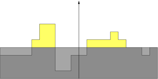
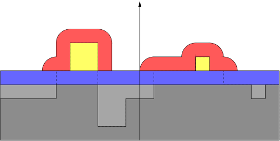
Figure 1. In dark gray the set $E\cap H_{\omega,s}$, in light gray the set $H_{\omega,s}\setminus E$, and in yellow the set $E\setminus H_{\omega,s}$.

Figure 2. In blue the set $H_{\omega,s+r}\setminus H_{\omega,s}$, and in red and yellow the set $(E+B_{r})\setminus H_{\omega,s+r}$.

We need also a second lemma, which is a crucial point in the proof of Theorem 1. The lemma states that the $r$-enlargement of a half-space $H_{s}$ cannot completely cover the $r$-enlargement of the set $E$, as depicted in Figures 2-2. This simple geometric fact is essentially due to the convexity of the half-space and therefore it is not surprising that a similar result holds also in the Euclidian case for the enlargement with a given convex set $K$ (see Lemma 4 in the next section).

Lemma 2.

For every $\omega\in\mathbb{S}^{n-1}$, $s\in\mathbb{R}$, $r\in(0,1]$, and for every subset $E\subset\mathbb{R}^{n}$ such that $\gamma(E)=\phi(s)$ the following estimate holds:

$$\gamma((E+B_{r})\setminus H_{\omega,s+r})\geq\frac{e^{-s^{+}}}{5}\,\gamma(E\setminus H_{\omega,s}).$$

Here $s^{+}=\max\{s,0\}$.

Proof.

We split the set $E$ in two parts: $E^{+}:=\{x\in E\colon\langle x,\omega\rangle\geq s+r\}$ and $E^{-}:=E\setminus E^{+}$. Of course

$$(E^{+}+B_{r})\setminus H_{\omega,s+r}\supset E^{+}\setminus H_{\omega,s+r}=E^{+}.$$ (9)

On the other hand, $E^{-}+B_{r}\supset E^{-}+r^{\prime}\omega$ for any $r^{\prime}\in(0,r)$ and

$$\begin{split}\gamma((E^{-}+r^{\prime}\omega)\setminus H_{\omega,s+r^{\prime}})&=\frac{1}{(2\pi)^{\frac{n}{2}}}\int_{(E^{-}+r^{\prime}\omega)\setminus H_{\omega,s+r^{\prime}}}e^{-\frac{|x|^{2}}{2}}dx\\ &=\frac{1}{(2\pi)^{\frac{n}{2}}}\int_{(E^{-})\setminus H_{\omega,s}}e^{-\frac{|x+r^{\prime}\omega|^{2}}{2}}dx\\ &\geq\frac{1}{(2\pi)^{\frac{n}{2}}}e^{-\frac{(3+2s^{+})}{2}}\int_{(E^{-})\setminus H_{\omega,s}}e^{-\frac{|x|^{2}}{2}}dx\\ &\geq\frac{e^{-s^{+}}}{5}\,\gamma(E^{-}\setminus H_{\omega,s}),\end{split}$$

since $|x+r^{\prime}\omega|^{2}\leq|x|^{2}+3+2s^{+}$ in $E^{-}$. Therefore, letting $r^{\prime}\to r$, we have

$$\gamma((E^{-}+B_{r})\setminus H_{\omega,s+r})\geq\frac{e^{-s^{+}}}{5}\,\gamma(E^{-}\setminus H_{\omega,s}).$$ (10)

Finally, from (9) and (10) we get

$$\begin{split}\gamma((E+B_{r})\setminus H_{\omega,s+r})=&\gamma((E^{+}+B_{r})\setminus H_{\omega,s+r})+\gamma((E^{-}+B_{r})\setminus H_{\omega,s+r})\\ \geq&\gamma(E^{+})+\frac{e^{-s^{+}}}{5}\,\gamma(E^{-}\setminus H_{\omega,s})\\ \geq&\frac{e^{-s^{+}}}{5}\,\gamma(E\setminus H_{\omega,s}).\end{split}$$

∎

Proof of Theorem 1.

Let us first show that we may assume

$$\gamma(E+B_{r})\leq\phi(s+r+1).$$ (11)

To this aim we first estimate

$$\phi(s+r+1)-\phi(s+r)=\frac{1}{\sqrt{2\pi}}\int_{s+r}^{s+r+1}e^{-\frac{t^{2}}{2}}\,dt\geq\frac{1}{\sqrt{2\pi}}e^{-\frac{(|s|+r+1)^{2}}{2}}.$$ (12)

On the other hand

$$\begin{split}\frac{\alpha_{\gamma}(E)}{2}\leq\phi(-|s|)&=\frac{1}{\sqrt{2\pi}}\int_{|s|}^{\infty}e^{-\frac{t^{2}}{2}}\,dt\\ &=\frac{1}{\sqrt{2\pi}}\left(\int_{|s|}^{|s|+1}e^{-\frac{t^{2}}{2}}\,dt+\int_{|s|+1}^{\infty}e^{-\frac{t^{2}}{2}}dt\right)\\ &\leq\frac{1}{\sqrt{2\pi}}\left(e^{-\frac{s^{2}}{2}}+\int_{|s|+1}^{\infty}te^{-\frac{t^{2}}{2}}dt\right)\\ &\leq\frac{1}{\sqrt{2\pi}}\left(e^{-\frac{s^{2}}{2}}+e^{-\frac{(|s|+1)^{2}}{2}}\right)\leq\frac{2}{\sqrt{2\pi}}e^{-\frac{s^{2}}{2}}.\end{split}$$ (13)

Assume now that (11) does not hold. Then we have by (12) and (13) that

$$\begin{split}\gamma(E+B_{r})-\phi(s+r)&\geq\phi(s+r+1)-\phi(s+r)\\ &\geq\frac{1}{\sqrt{2\pi}}e^{-\frac{(|s|+r+1)^{2}}{2}}\\ &\geq c\,e^{s^{2}}e^{-\frac{(|s|+r+1)^{2}}{2}}\alpha_{\gamma}^{2}(E).\end{split}$$

Hence if (11) does not hold then (2) is true.

Because of the non-monotonicity of the quantity $\gamma(E+B_{r})-\phi(s+r)$, we have to divide the rest of the proof in several steps. We first prove the theorem when $r\in(0,1]$. We divide this part of the proof in two cases.

Case 1. We first assume that for all $\rho\in(0,r]$ it holds

$$\gamma(E+B_{\rho})-\phi(s+\rho)\leq\varepsilon\,e^{\frac{s^{2}}{2}}e^{-3|s|}\alpha_{\gamma}^{2}(E),$$ (14)

where $\varepsilon>0$ is a small number to be chosen later.

We define an auxiliary function $f:(0,r)\to\mathbb{R}$ by

$$f(\rho):=P_{\gamma}(E+B_{\rho})-e^{-(s+\rho)^{2}/2}.$$

Then by Lemma 1

$$\gamma(E+B_{r})-\phi(s+r)\geq\frac{1}{\sqrt{2\pi}}\int_{0}^{r}f(\rho)d\rho.$$

Therefore in order to prove (2), it is enough to estimate $f(\rho)$. Let us fix $\rho\in(0,r)$. Let $\hat{\rho}>0$ be such that $\gamma(E+B_{\rho})=\phi(s+\hat{\rho})$. Note that by the concentration inequality $\hat{\rho}\geq\rho$. Moreover (11) implies that $\hat{\rho}\leq 2$.

Let $\omega_{\rho}\in\mathbb{S}^{n-1}$ be a direction that realizes $\min_{\omega\in\mathbb{S}^{n-1}}\gamma((E+B_{\rho})\triangle H_{\omega,s+\hat{\rho}})$, and let $s^{-}=-\min\{s,0\}$. By the stability of the Gaussian isoperimetric inequality (8) and by Lemma 2 we have

$$\begin{split}f(\rho)&=\left(P_{\gamma}(E+B_{\rho})-e^{-\frac{(s+\hat{\rho})^{2}}{2}}\right)+e^{-\frac{(s+\hat{\rho})^{2}}{2}}-e^{-\frac{(s+\rho)^{2}}{2}}\\ &\geq c\,\frac{e^{\frac{(s+\hat{\rho})^{2}}{2}}}{1+(s+\hat{\rho})^{2}}\,\gamma((E+B_{\rho})\triangle H_{\omega_{\rho},s+\hat{\rho}})^{2}+e^{-\frac{(s+\hat{\rho})^{2}}{2}}-e^{-\frac{(s+\rho)^{2}}{2}}\\ &\geq c\,\frac{e^{\frac{s^{2}}{2}}e^{-2s^{-}}}{(1+s^{2})}\,\bigl{(}\gamma((E+B_{\rho})\setminus H_{\omega_{\rho},s+\rho})-\gamma(H_{\omega_{\rho},s+\hat{\rho}}\setminus H_{\omega_{\rho},s+\rho})\bigr{)}^{2}+e^{-\frac{(s+\hat{\rho})^{2}}{2}}-e^{-\frac{(s+\rho)^{2}}{2}}\\ &\geq c\,\frac{e^{\frac{s^{2}}{2}}e^{-2s^{-}}}{(1+s^{2})}\,\Bigl{(}\frac{e^{-s^{+}}}{10}\alpha_{\gamma}(E)-\gamma(H_{\omega_{\rho},s+\hat{\rho}}\setminus H_{\omega_{\rho},s+\rho})\Bigr{)}^{2}+e^{-\frac{(s+\hat{\rho})^{2}}{2}}-e^{-\frac{(s+\rho)^{2}}{2}}.\end{split}$$

By the definition of $\hat{\rho}$, by (14) and by (13) we have

$$\begin{split}\gamma(H_{\omega_{\rho},s+\hat{\rho}}\setminus H_{\omega_{\rho},s+\rho})&=\gamma(E+B_{\rho})-\phi(s+\rho)\\ &\leq\varepsilon\,e^{\frac{s^{2}}{2}}e^{-3|s|}\alpha_{\gamma}^{2}(E)\leq\frac{e^{-3|s|}}{20}\alpha_{\gamma}(E)\end{split}$$

when $\varepsilon$ is small enough. We use (14) to estimate

$$\begin{split}e^{-\frac{(s+\hat{\rho})^{2}}{2}}-e^{-\frac{(s+\rho)^{2}}{2}}&=-\int_{s+\rho}^{s+\hat{\rho}}te^{-\frac{t^{2}}{2}}dt\geq-(|s|+2)\int_{s+\rho}^{s+\hat{\rho}}e^{-\frac{t^{2}}{2}}dt\\ &=-\sqrt{2\pi}\,(|s|+2)\left(\gamma(E+B_{\rho})-\phi(s+\rho)\right)\\ &\geq-\varepsilon\,\sqrt{2\pi}\,(|s|+2)e^{\frac{s^{2}}{2}}e^{-3|s|}\alpha_{\gamma}^{2}(E).\end{split}$$

Therefore by the previous three estimates we have

$$\begin{split}f(\rho)&\geq c\,\frac{e^{\frac{s^{2}}{2}}e^{-2|s|}}{(1+s^{2})}\,\alpha_{\gamma}^{2}(E)-\varepsilon\,\sqrt{2\pi}\,(|s|+2)e^{\frac{s^{2}}{2}}e^{-3|s|}\alpha_{\gamma}^{2}(E).\\ &\geq c\,e^{\frac{s^{2}}{2}}e^{-3|s|}\,\alpha_{\gamma}^{2}(E)\end{split}$$

when $\varepsilon$ is small enough. Thus we have the claim (2) in this case.

Case 2. In this case we assume that there is $\rho\in(0,r]$ such that

$$\gamma(E+B_{\rho})-\phi(s+\rho)\geq\varepsilon\,e^{\frac{s^{2}}{2}}e^{-3|s|}\alpha_{\gamma}^{2}(E).$$ (15)

Let $\hat{\rho}>0$ be such that

$$\gamma(E+B_{\rho})=\phi(s+\hat{\rho}).$$

The concentration inequality implies

$$\gamma(E+B_{r})\geq\phi(s+\hat{\rho}+r-\rho).$$ (16)

Note that (11) gives $\hat{\rho}\leq 2$. We may therefore estimate

$$\begin{split}\phi(s+\hat{\rho}+r-\rho)-\phi(s+r)&=\frac{1}{\sqrt{2\pi}}\int_{s+r}^{s+\hat{\rho}+r-\rho}e^{-\frac{t^{2}}{2}}\,dt=\frac{1}{\sqrt{2\pi}}\int_{s+\rho}^{s+\hat{\rho}}e^{-\frac{(t+r-\rho)^{2}}{2}}\,dt\\ &\geq c\,e^{-s^{+}}\int_{s+\rho}^{s+\hat{\rho}}e^{-\frac{t^{2}}{2}}\,dt=c\,e^{-s^{+}}(\phi(s+\hat{\rho})-\phi(s+\rho)).\end{split}$$

We deduce from (16), from the definition of $\hat{\rho}$ and from (15) that

$$\gamma(E+B_{r})-\phi(s+r)\geq c\,e^{-s^{+}}(\gamma(E+B_{\rho})-\phi(s+\rho))\geq c\,\varepsilon\,e^{\frac{s^{2}}{2}}e^{-4|s|}\alpha_{\gamma}^{2}(E),$$

which proves the claim (2).

We are left to prove the claim (2) when $r>1$. Since we have already proved the result for $r=1$ we have that

$$\gamma(E+B_{1})-\phi(s+1)\geq c_{1}\,e^{\frac{s^{2}}{2}}e^{-\frac{(|s|+5)^{2}}{2}}\alpha_{\gamma}^{2}(E),$$

for an absolute constant $c_{1}>0$. The rest of the proof is the same as in the Case 2 above. Let $\hat{\rho}\geq 1$ be such that

$$\gamma(E+B_{1})=\phi(s+\hat{\rho}).$$

The concentration inequality implies

$$\gamma(E+B_{r})\geq\phi(s+\hat{\rho}+r-1).$$

Note that (11) and the above inequality give $\hat{\rho}\leq 2$ and we may estimate as before

$$\begin{split}\phi(s+\hat{\rho}+r-1)-\phi(s+r)&=\frac{1}{\sqrt{2\pi}}\int_{s+r}^{s+\hat{\rho}+r-1}e^{-\frac{t^{2}}{2}}\,dt\\ &\geq\frac{1}{\sqrt{2\pi}}\,e^{-(|s|+1)(r-1)}\,e^{-\frac{r^{2}}{2}}\int_{s+1}^{s+\hat{\rho}}e^{-\frac{t^{2}}{2}}\,dt\\ &=e^{-(|s|+1)(r-1)}\,e^{-\frac{r^{2}}{2}}(\phi(s+\hat{\rho})-\phi(s+1)).\end{split}$$

The four estimates above yield

$$\gamma(E+B_{r})-\phi(s+r)\geq c_{1}\,e^{s^{2}}e^{-\frac{(|s|+5)^{2}}{2}}e^{-(|s|+1)(r-1)}e^{-\frac{r^{2}}{2}}\,\alpha_{\gamma}^{2}(E)$$

and the claim (2) follows. ∎

Remark 1.

The best known value for the constant $c$ in the isoperimetric estimate (8) is $c_{\text{iso}}=1/(48\sqrt{2\pi})$, obtained by a slightly refinement of the argument in [1]. A careful study of the proof of Theorem 1 shows that one can take the value for the constant $c$ in (2) to be $c_{\text{iso}}/2000$. In both the cases the values are not optimal.

3. The Euclidean concentration

In this section we provide a proof of Theorem 2. The symbol $c_{n}$ will denote a positive constant depending on $n$, whose value is not specified and which may vary from line to line.

The proof of Theorem 2 is based on the quantitative Wulff inequality provided in [11]. Let us briefly introduce some notation. We set

$$||\nu||_{*}=\sup_{x\in K}\langle x,\nu\rangle,\qquad\nu\in\mathbb{S}^{n-1}$$

and define the anisotropic perimeter for a set $E$ with locally finite perimeter as

$$P_{K}(E)=\int_{\partial^{*}E}||\nu||_{*}\,d\mathcal{H}^{n-1},$$

where $\partial^{*}E$ denotes the reduced boundary of $E$. When $E$ is open with Lipschitz boundary we have

$$P_{K}(E)=\lim_{r\to 0}\frac{|E+rK|-|E|}{r}.$$

The result in [11] states that for every set $E$ of locally finite perimeter with $|E|=|sK|$ it holds

$$P_{K}(E)-P_{K}(sK)\geq\frac{c_{n}}{|K|}\frac{1}{s^{n+1}}\alpha^{2}(E).$$ (17)

The following lemma is the counterpart of Lemma 1 in the Euclidean case.

Lemma 3.

Let $r>0$ and let $E$ be a measurable set such that $|E+rK|<\infty$. Then

$$|E+rK|\geq|E|+\int_{0}^{r}P_{K}(E+\rho K)\,d\rho.$$

Similarly to Lemma 2, the measure of $E\setminus K$ is increasing along the growth.

Lemma 4.

Let $E\subset\mathbb{R}^{n}$ be a measurable set such that $|E|=|K|$. Then for every $r>0$ it holds

$$|(E+rK)\setminus(1+r)K|\geq|E\setminus K|.$$

Proof.

Let $r_{0}\geq 1$ be such that $|E\cup K|=|r_{0}K|$. Then

$$|E\setminus K|=|E\cup K|-|K|=(r_{0}^{n}-1)|K|.$$ (18)

By the concentration inequality (3) it holds

$$|(E\cup K)+rK|\geq|(r_{0}+r)K|.$$

Since $[(E+rK)\setminus(1+r)K]\cup(1+r)K=(E\cup K)+rK$, one has

$$|(E\cup K)+rK|-|(1+r)K|=|(E+rK)\setminus(1+r)K|.$$

These together yield

$$\begin{split}|(E+rK)\setminus(1+r)K|&\geq|(r_{0}+r)K|-|(1+r)K|\\ &=((r+r_{0})^{n}-(1+r)^{n})|K|\geq(r_{0}^{n}-1)|K|,\end{split}$$

where the last inequality follows from the fact that $t\mapsto((t+r_{0})^{n}-(1+t)^{n})$ is nondecreasing. The claim then follows from (18). ∎

Proof of Theorem 2.

By scaling we may assume that $|K|=1$. Let us first prove the claim when $r\in(0,1]$. We may assume that $|E+rK|\leq|3K|$. Indeed if $|E+rK|>|3K|$ then

$$|E+rK|-|(1+r)K|>|3K|-|2K|=3^{n}-2^{n}\geq\frac{3^{n}-2^{n}}{4}\alpha^{2}(E).$$

Let us define $f:(0,r)\to\mathbb{R}$,

$$f(\rho)=P_{K}(E+\rho K)-P_{K}((1+\rho)K).$$

By Lemma 3 we have that $f(\rho)<\infty$ for almost every $\rho$. By the concentration inequality (3) it holds $|E+\rho K|\geq|(1+\rho)K|$ for every $\rho\in(0,r)$. Let us fix $\rho<r$ and let $\hat{\rho}\geq\rho$ be such that $|(1+\hat{\rho})K|=|E+\rho K|$. Then by $|E+rK|\leq|3K|$ we have $\hat{\rho}\leq 2$. By the stability of the Wulff inequality (17) and recalling that $P_{K}(\lambda K)=n\lambda^{n-1}|K|$ for every $\lambda>0$, we have

$$\begin{split}f(\rho)&=\left[P_{K}(E+\rho K)-P_{K}((1+\hat{\rho})K)\right]+\left[P_{K}((1+\hat{\rho})K)-P_{K}((1+\rho)K)\right]\\ &\geq c_{n}\Bigl{(}\inf_{x\in\mathbb{R}^{n}}|((E+\rho K)+x)\triangle(1+\hat{\rho})K|\Bigr{)}^{2}+n\left((1+\hat{\rho})^{n-1}-(1+\rho)^{n-1}\right).\end{split}$$

We estimate the last term by

$$(1+\hat{\rho})^{n-1}-(1+\rho)^{n-1}\geq\frac{(1+\hat{\rho})^{n}-(1+\rho)^{n}}{2+\rho+\hat{\rho}}\geq\frac{1}{5}\left(|(1+\hat{\rho})K|-|(1+\rho)K|\right).$$

Thus it holds

$$\begin{split}f(\rho)&\geq c_{n}\left(\inf_{x\in\mathbb{R}^{n}}|((E+\rho K)+x)\triangle(1+\hat{\rho})K|\right)^{2}+\frac{n}{5}\left(|(1+\hat{\rho})K|-|(1+\rho)K|\right)\\ &\geq c_{n}\left(\inf_{x\in\mathbb{R}^{n}}|((E+\rho K)+x)\setminus(1+\hat{\rho})K|\right)^{2}+c_{n}\left(|(1+\hat{\rho})K|-|(1+\rho)K|\right)^{2}\\ &\geq c_{n}\left(\inf_{x\in\mathbb{R}^{n}}|((E+\rho K)+x)\setminus(1+\rho)K|\right)^{2},\end{split}$$

where the last inequality is a simple consequence of

$$|((E+\rho K)+x)\setminus(1+\rho)K|\leq|((E+\rho K)+x)\setminus(1+\hat{\rho})K|+|(1+\hat{\rho})K\setminus(1+\rho)K|.$$

Now we use Lemma 4 and deduce that for every $\rho\in(0,r)$ it holds

$$\inf_{x\in\mathbb{R}^{n}}|(E+\rho K)+x)\setminus(1+\rho)K|\geq\frac{\alpha(E)}{2}.$$

Hence we conclude that

$$f(\rho)\geq c_{n}\,\alpha^{2}(E)$$

for every $\rho\in(0,r)$ and the result follows by Lemma 3.

Let us assume $r>1$. By the previous argument we have

$$|E+K|-|2K|\geq c_{n}\,\alpha^{2}(E).$$ (19)

By choosing $c_{n}\leq 1/4$ we may assume that $c_{n}\,\alpha^{2}(E)\leq 1$. Thus we have the elementary inequality $2^{n}+c_{n}\,\alpha^{2}(E)\geq(2+c_{n}\,\alpha^{2}(E)/(n3^{n}))^{n}$. Therefore, by (19) we have $|E+K|\geq|(2+c_{n}\,\alpha^{2}(E))K|$ for a possibly smaller $c_{n}$. Using this estimate and the concentration inequality (3) we get

$$|(E+K)+(r-1)K|\geq|(1+r+c_{n}\,\alpha^{2}(E))K|.$$

Thus we conclude that

$$|E+rK|-|(1+r)K|\geq|(1+r+c_{n}\,\alpha^{2}(E))K|-|(1+r)K|\geq c_{n}(1+r)^{n-1}\alpha^{2}(E).$$

∎

Remark 2.

The constant $c_{n}$ in the isoperimetric estimate (17) decays at most like $n^{-13}$ as $n\to\infty$. Instead, a careful study of the proof of Theorem 2 shows that the value for the constant $c_{n}$ in (5) decays at most like $9^{-n}$. Both these decays do not seem optimal. In particular, for (17) we conjectured that the constant $c_{n}$ is in fact independent of the dimension.

Proof of Corollary 1.

We may assume that $|E+F|\leq 3^{n}\max\{|E|,|F|\}$, since otherwise (6) is trivially true. Let $s>0$ be such that $|E|=|sF|$. The concentration inequality (3) implies $|E+F|\geq|(1+s)F|$. Therefore,

$$\begin{split}|E+F|^{1/n}-|E|^{1/n}-|F|^{1/n}&=|E+F|^{1/n}-|(1+s)F|^{1/n}\\ &\geq\frac{1}{n|E+F|^{(n-1)/n}}[|E+F|-|(1+s)F|]\\ &\geq c_{n}\left(\frac{1}{\max\{|E|,|F|\}}\right)^{(n-1)/n}[|E+F|-|(1+s)F|].\end{split}$$

Assume first $|E|\geq|F|$. By (5) with $K=sF$ and $r=1/s$ we get,

$$\begin{split}|E+F|^{1/n}-|E|^{1/n}-|F|^{1/n}&\geq\frac{c_{n}}{s|E|^{(n-1)/n}}\,\frac{\alpha^{2}(E,F)}{|E|}\\ &=c_{n}\,|F|^{1/n}\,\frac{\alpha^{2}(E,F)}{|E|^{2}}.\end{split}$$

On the other hand when $|F|\geq|E|$, the same argument yields

$$\begin{split}|E+F|^{1/n}-|E|^{1/n}-|F|^{1/n}&\geq\frac{c_{n}}{s^{n-1}|F|^{(n-1)/n}}\,\frac{\alpha^{2}(E,F)}{|E|}\\ &=c_{n}\,|E|^{1/n}\,\frac{\alpha^{2}(E,F)}{|E|^{2}}.\end{split}$$

∎

References

- [1] M. Barchiesi, A. Brancolini & V. Julin. Sharp dimension free quantitative estimates for the Gaussian isoperimetric inequality. Ann. Probab., 45, 668–697 (2017).
- [2] E. A. Carlen & C. Kerce. On the cases of equality in Bobkov’s inequality and Gaussian rearrangement. Calc. Var. Partial Differential Equations 13, 1–18 (2001).
- [3] E. Carlen & F. Maggi. Stability for the Brunn-Minkowski and Riesz rearrangement inequalities, with applications to Gaussian concentration and finite range non-local isoperimetry. To appear in Canadian J. Math., DOI: 10.4153/CJM-2016-026-9
- [4] A. Cianchi, N. Fusco, F. Maggi & A. Pratelli. On the isoperimetric deficit in Gauss space. Amer. J. Math. 133, 131–186 (2011).
- [5] M. Christ. Near equality in the Brunn-Minkowski inequality. Preprint (2012), http://arxiv.org/abs/1207.5062
- [6] R. Eldan. A two-sided estimate for the Gaussian noise stability deficit. Invent. Math. 201, 561–624 (2015).
- [7] R. Eldan & B. Klartag. Dimensionality and the stability of the Brunn-Minkowski inequality. Ann. Sc. Norm. Super. Pisa Cl. Sci. (5), 13, 975–1007 (2014).
- [8] A. Figalli & D. Jerison. Quantitative stability of the Brunn-Minkowski inequality. To appear in Adv. Math..
- [9] A. Figalli & D. Jerison. Quantitative stability for sumsets in . J. Eur. Math. Soc., 17, 1079–1106 (2015).
- [10] A. Figalli, F. Maggi & C. Mooney. The sharp quantitative Euclidean concentration inequality. Preprint (2016), https://arxiv.org/abs/1601.04100
- [11] A. Figalli, F. Maggi & A. Pratelli. A mass transportation approach to quantitative isoperimetric inequalities. Invent. Math. 182, 167–211 (2010).
- [12] A. Figalli, F. Maggi & A. Pratelli. A refined Brunn-Minkowski inequality for convex sets. Ann. Inst. H. Poincaré Anal. Non Linéaire, 26, 2511–2519 (2009).
- [13] R. J. Gardner. The Brunn-Minkowski inequality. Bull. Amer. Math. Soc. (N.S.), 39, 355–405 (2002).
- [14] M. Ledoux. Isoperimetry and Gaussian analysis. In Lectures on probability theory and statistics, volume 1648 of Lecture Notes in Math., pages 165–294. Springer, Berlin, (2006).
- [15] M. Ledoux. Concentration of measure and logarithmic Sobolev inequalities. In Séminaire de Probabilités XXXIII, volume 1709 of Lecture Notes in Math., pages 120–216. Springer, Berlin, (2006).
- [16] F. Maggi. Sets of finite perimeter and geometric variational problems. An introduction to geometric measure theory. Cambridge Studies in Advanced Mathematics, 135. Cambridge University Press, Cambridge (2012).
- [17] E. Mossel & J. Neeman. Robust Dimension Free Isoperimetry in Gaussian Space. Ann. Probab. 43, 971–991 (2015).
- [18] E. Mossel & J. Neeman. Robust optimality of Gaussian noise stability. J. Eur. Math. Soc. 17, 433–482 (2015).