Geometric adaptive Monte Carlo in random environment

Abstract

Manifold Markov chain Monte Carlo algorithms have been introduced to sample more effectively from challenging target densities exhibiting multiple modes or strong correlations. Such algorithms exploit the local geometry of the parameter space, thus enabling chains to achieve a faster convergence rate when measured in number of steps. However, acquiring local geometric information can often increase computational complexity per step to the extent that sampling from high-dimensional targets becomes inefficient in terms of total computational time. This paper analyzes the computational complexity of manifold Langevin Monte Carlo and proposes a geometric adaptive Monte Carlo sampler aimed at balancing the benefits of exploiting local geometry with computational cost to achieve a high effective sample size for a given computational cost. The suggested sampler is a discrete-time stochastic process in random environment. The random environment allows to switch between local geometric and adaptive proposal kernels with the help of a schedule. An exponential schedule is put forward that enables more frequent use of geometric information in early transient phases of the chain, while saving computational time in late stationary phases. The average complexity can be manually set depending on the need for geometric exploitation posed by the underlying model.

Theodore Papamarkou^1,2, Alexey Lindo², Eric B. Ford^3,4,5,6

¹Department of Mathematics

The University of Manchester, Manchester, M13 9PL, UK

²School of Mathematics and Statistics

University of Glasgow, Glasgow, G12 8QQ, UK

³Department of Astronomy and Astrophysics

525 Davey Laboratory, The Pennsylvania State University, University Park, PA, 16802, USA

⁴Center for Exoplanets and Habitable Worlds

525 Davey Laboratory, The Pennsylvania State University, University Park, PA, 16802, USA

⁵Center for Astrostatistics

525 Davey Laboratory, The Pennsylvania State University, University Park, PA 16802, USA

⁶Institute for Computational and Data Sciences

525 Davey Laboratory, The Pennsylvania State University, University Park, PA 16802, USA

1 Introduction

Geometric Markov chain Monte Carlo (MCMC) dates back to the work of [9], which introduced Hamiltonian Monte Carlo (HMC) to unite MCMC with molecular dynamics. Statistical applications of HMC began with its use in neural network models by [33].

In the meanwhile, the Metropolis-adjusted Langevin algorithm (MALA) was proposed by [39] to employ Langevin dynamics for MCMC sampling. Both HMC and MALA evaluate the gradient of the target density, so they utilize local geometric flow.

[15] introduced new differential geometric MCMC methods. Given a state $\theta\in\mathbb{R}^{n}$, [15] defines a distance between two probability densities $p(\theta)$ and $p(\theta+\delta\theta)$ as the quadratic form $\delta\theta^{T}M(\theta)\delta\theta$ for an arbitrary metric $M(\theta)$. Thus, the position-specific metric $M(\theta)$ induces a Riemann manifold in the space of parameterized probability density functions $\left\{p(\theta):\theta\right\}$. [15] uses $M(\theta)$ to define proposal kernels that explore the state space $\left\{\theta:\theta\in\mathbb{R}^{n}\right\}$ effectively by introducing Riemann manifold Langevin and Hamiltonian Monte Carlo methods.

Computing the geometric entities of differential geometric MCMC methods creates a performance bottleneck that restricts the applicability of the involved methods. For example, manifold MCMC methods require to calculate the metric tensor $M(\theta)$ of choice. Typically, $M(\theta)$ is set to be the observed Fisher information matrix, which equals the negative Hessian of the log-target density at state $\theta$. Consequently, the complexity of manifold MCMC algorithms is dominated by Hessian-related computations, such as the gradient of or the inverse of the Hessian.

[15] constructed the simplified manifold Metropolis-adjusted Langevin algorithm (SMMALA) that is of the same order of complexity per Monte Carlo iteration but faster than MMALA and RMHMC for target distributions of low complexity. The faster speed of SMMALA over MMALA and RMHMC is explained by lower order terms and constant factors appearing in big-oh notation, which are ordinarily omitted but affect runtime in the case of less costly targets.

SMMALA has been used in conjunction with population MCMC for the Bayesian analysis of mechanistic models based on systems of non-linear differential equations, see [5, 45]. Despite the capacity of SMMALA to exploit local geometric information so as to cope with non-linear correlations and modest increase in the complexity of the target density, in case of more expensive targets its computational complexity can render performance inferior to other algorithms such as the Metropolis-adjusted Langevin algorithm (MALA) or adaptive MCMC, see [4].

Various attempts have been made to ameliorate the computational implications of geometric MCMC methods. Along these lines, [29] used Gaussian processes to emulate the Hessian matrix and Christoffel symbols associated with the observed Fisher information $M(\theta)$. [7] developed a stochastic quasi-Newton Langevin Monte Carlo algorithm which takes into account the local geometry, while approximating the inverse Hessian by using a limited history of samples and their gradients. Alternatively, [37] used convex analysis and proximal techniques instead of differential calculus in order to construct a Langevin Monte Carlo method for high-dimensional target distributions that are log-concave and possibly not continuously differentiable.

The present paper serves two purposes. Initially, it studies the computational complexity of geometric Langevin Monte Carlo algorithms. Subsequently, it develops the so-called geometric adaptive Monte Carlo (GAMC) sampling scheme based on a random environment of geometric and adaptive proposal kernels. For expensive targets, a carefully selected random environment of a local geometric Langevin kernel and of adaptive Metropolis kernels can give rise to a sampler with higher sampling efficacy than a sampler based on the local geometric Langevin kernel alone.

2 Background

The role of this section is to provide a brief overview of Langevin Monte Carlo and of adaptive Metropolis, which will be combined in later sections to construct a Monte Carlo sampling method in random environment.

To establish notation, consider a Polish space $E$ equipped with the Borel $\sigma$-algebra $\mathcal{E}$. Let $\{\theta_{k}\}$ be a sequence in $E$ and

$$\theta_{w:z}:=\left(\theta_{w},\theta_{w+1},\ldots,\theta_{z}\right),~{}w\leq z,$$

a subsequence of $\{\theta_{k}\}$, where $k$, $w$ and $z$ denote non-negative integers. Moreover, let $Q\colon E^{z-w+1}\times\mathcal{E}\rightarrow\mathbb{R}_{+}$ be a kernel from $E^{z-w+1}$ to $E$.

It is assumed that for every subsequence $\theta_{w:z}$ of $\{\theta_{k}\}$, measure $Q(\theta_{w:z},\cdot)$ is absolutely continuous with respect to some measure $\nu$ on $(E^{z-w+1},\mathcal{E}^{z-w+1})$. Such an assumption ensures existence of the Radon-Nikodym derivative $q_{\theta_{w:z}}$ so that

$$Q(\theta_{w:z},B)=\int_{B}q_{\theta_{w:z}}d\nu$$ (1)

for any $B\in\mathcal{E}$.

The Radon-Nikodym derivative $q_{\theta_{w:z}}$ is used in the paper as a proposal density in geometric or adaptive Monte Carlo methods to sample from a possibly unnormalized target density $p\colon E\rightarrow\mathbb{R}_{+}$. In the context of Monte Carlo sampling, $\{\theta_{k}\}$ and $Q$ are called chain and proposal kernel, respectively.

2.1 Basics of Langevin Monte Carlo

Langevin Monte Carlo (LMC) is a case of Metropolis-Hastings. The normal proposal density at the $k$-th iteration of LMC is given by

$$g_{\theta_{k}}(\theta^{\star}):=\mathcal{N}(\theta^{\star}|\mu(\theta_{k},M,\epsilon),\Sigma(M,\epsilon)),$$ (2)

where $\theta_{k}$ and $\theta^{\star}$ denote the state at the $k$-th iteration and the proposed state, respectively. $M$ is a positive definite matrix of size $n\cdot n$ and $\epsilon$ refers to a tuning parameter known as the integration stepsize. The location $\mu(\theta_{k},M,\epsilon)$ is a function of $\theta_{k}$, $M$ and $\epsilon$, whereas the covariance $\Sigma(M,\epsilon)$ of the proposal kernel depends on $M$ and $\epsilon$. Both $\mu(\theta_{k},M,\epsilon)$ and $\Sigma(M,\epsilon)$ are defined so that the proposed states admit a Langevin diffusion approximated by a first-order Euler discretization. The Metropolis-Hastings acceptance probability is set to its standard form

$$r_{g}(\theta_{k},\theta^{\star}):=\min\left\{\frac{p(\theta^{\star})g_{\theta^{\star}}(\theta_{k})}{p(\theta_{k})g_{\theta_{k}}(\theta^{\star})},1\right\}$$ (3)

if $p(\theta_{k})g_{\theta_{k}}(\theta^{\star})>0$, and $r_{g}(\theta,\theta^{\star}):=1$ otherwise.

The proposal kernel $G(\theta_{k},\cdot)$ corresponding to the normal density $g_{\theta_{k}}$ of equation (2) is defined by setting $E=\mathbb{R}^{n}$, $w=z=k$, $q_{\theta_{w:z}}=g_{\theta_{k}}$ and $\nu$ to be the Lebesgue measure in equation (1).

The integration stepsize $\epsilon$, also known as drift step, is associated with the first order Euler discretization and significantly affects the rate of state space exploration. If $\epsilon$ is selected to be relatively large, many of the proposed candidates will be far from the current state, and are likely to have a low probability of acceptance, so the chain with proposal kernel $G$ will have low acceptance rate. Reducing $\epsilon$ will increase the acceptance rate, but the chain will take longer to traverse the state space.

In a Bayesian setting, the target is a possibly unnormalized posterior density $p(\cdot|y)$, where $y$ denotes the available data. Replacing $p(\cdot)$ by $p(\cdot|y)$ in (3) makes Langevin Monte Carlo applicable in Bayesian problems.

To fully specify a Langevin Monte Carlo algorithm, the location $\mu(\theta_{k},M,\epsilon)$ and covariance $\Sigma(M,\epsilon)$ of normal proposal (2) need to be defined. In what follows, variations of geometric Langevin Monte Carlo methods are distinguished by their respective proposal location and covariance.

2.2 Metropolis-adjusted Langevin algorithm

If $M$ is not a function of the state $\theta_{k}$, the Metropolis-adjusted Langevin algorithm (MALA) arises as

$$\mu(\theta_{k},M,\epsilon) =\theta_{k}+\frac{\epsilon^{2}}{2}M^{-1}\nabla\log{p(\theta_{k})},$$ (4)

$$\Sigma(M,\epsilon) =\epsilon^{2}M^{-1}.$$ (5)

$M$ is known as the precondition matrix, see [42]. It is typically set to be the identity matrix $M=I$, in which case MALA is defined in its conventional form.

MALA uses the gradient flow $\nabla\log{p(\theta)}$ to make proposals effectively. According to the theoretical analysis of [39], the optimal scaling $\epsilon$ has been found to be the value of $\epsilon$ which yields a limiting acceptance rate of $57.4\%$ in high-dimensional parametric spaces (as $n\rightarrow\infty$).

2.3 Manifold Langevin Monte Carlo

It is possible to incorporate further geometric structure in the form of a position-dependent metric $M(\theta_{k})$, see [15, 51]. The Langevin diffusion is defined on a Riemann manifold endowed by the metric $M(\theta_{k})$. At the $k$-th iteration of the associated manifold Metropolis-adjusted Langevin algorithm (MMALA), candidate states are drawn from a normal proposal density with location and covariance given by

$$\mu(\theta_{k},M(\theta),\epsilon) =\theta_{k}+\displaystyle\frac{\epsilon^{2}}{2}M^{-1}(\theta_{k})\nabla\log{p(\theta_{k})}+\epsilon^{2}\boldsymbol{\gamma}(\theta_{k}),$$ (6)

$$\Sigma(M(\theta_{k}),\epsilon) =\epsilon^{2}M^{-1}(\theta_{k}),$$ (7)

where the $i$-th coordinate $\gamma_{i}(\theta_{k})$ of $\boldsymbol{\gamma}(\theta_{k})\in\mathbb{R}^{n}$ is

$$\begin{split}\gamma_{i}(\theta_{k})&=\displaystyle\frac{1}{2}\sum_{j=1}^{n}\frac{\partial M^{-1}_{ij}(\theta_{k})}{\partial(\theta_{k})_{j}}\\ &=-\displaystyle\frac{1}{2}\sum_{j,h,l=1}^{n}M^{-1}_{ih}(\theta_{k})\frac{\partial M_{hl}(\theta_{k})}{\partial(\theta_{k})_{j}}M^{-1}_{lj}(\theta_{k}).\end{split}$$ (8)

$(\theta_{k})_{j}$, $M_{hl}(\theta_{k})$ and $M^{-1}_{ij}(\theta_{k})$ in (8) denote the respective $j$-th coordinate of $\theta_{k}$, $(h,l)$-th element of $M(\theta_{k})$ and $(i,j)$-th element of $M^{-1}(\theta_{k})$.

As seen from (8), the term $\boldsymbol{\gamma}(\theta_{k})$ increases the computational complexity of operations on the proposal density for target densities with high number $n$ of dimensions or with high correlation between parameters. To reduce the computational cost, $\boldsymbol{\gamma}(\theta_{k})$ can be dropped from (6), simplifying the proposal location to

$$\mu(\theta_{k},M(\theta_{k}),\epsilon)=\theta_{k}+\frac{\epsilon^{2}}{2}M^{-1}(\theta_{k})\nabla\log{p(\theta_{k})}.$$ (9)

The method with location and covariance specified by (9) and (7) is known as simplified Metropolis-adjusted Langevin algorithm (SMMALA).

The optimal stepsize $\epsilon$ for MMALA and SMMALA is empirically suggested by [15] to be set so as to obtain an acceptance rate of around $70\%$; this choice has not been analyzed yet from a theoretical standpoint analogously to the choice of scaling for MALA by [39].

2.4 Synopsis of Langevin Monte Carlo algorithms

The proposal mechanisms of MALA, SMMALA and MMALA define valid MCMC methods that converge to the target distribution. In fact, if the metric $M(\theta_{k})$ is constant, then $\boldsymbol{\gamma}(\theta_{k})$ vanishes, so each of SMMALA and MMALA coincides with pre-conditioned MALA.

Each of the three Langevin Monte Carlo samplers incorporate different amount of local geometry in the proposal mechanism. MALA makes use only of the gradient of the log-target. SMMALA relies additionally on the position-specific metric tensor $M(\theta_{k})$. MMALA takes into account the curvature of the manifold induced by $M(\theta_{k})$, which implies calculating the metric derivatives $\partial M_{hl}(\theta_{k})/\partial(\theta_{k})_{j}$ in (8). Depending on the manifold and its curvature, the proposals of the three Langevin Monte Carlo samplers may exhibit varying efficiency in converging to the target distribution, thus leading to differences in effective sample size.

Increasing inclusion of local geometry in the proposal mechanism escalates computational complexity. More specifically, MALA, SMMALA and MMALA require computing first, second and third order derivatives of the target. It is thus clear that there is a trade-off between geometric exploitation of the target from within the proposal density and associated complexity of the proposal density, which translates to a trade-off between effective sample size and runtime for MALA, SMMALA and MMALA.

2.5 Basics of adaptive Metropolis

Sampling methods that propose samples by using past values of the chain, thus breaking the Markov property, are referred to as adaptive Monte Carlo. The first adaptive Metropolis (AM) algorithm, as introduced by [20], used a proposal kernel based on the empirical covariance matrix of the whole chain at each iteration.

In its first appearance in [20], the AM algorithm was defined for target densities of bounded support to ensure convergence. [41] extended AM to work with targets of unbounded support by suggesting a mixture proposal density also based on the empirical covariance matrix of the whole chain at each iteration.

Several variations of the AM algorithm have appeared. For example, [19] combined adaptive Metropolis and delayed rejection methodology to construct the delayed rejection adaptive Metropolis (DRAM) sampler, which outperforms its constituent methods in certain situations. More recently, [48] introduced the so-called robust adaptive Metropolis (RAM) algorithm, which scales the empirical covariance matrix of the chain to yield a desired mean acceptance rate, typically $23.4\%$ in multidimensional settings. A thorough overview of adaptive Metropolis methods can be found in [18].

The ergodicity properties of adaptive Monte Carlo were studied in [1, 40]. In particular, [40] defined the diminishing adaptation and bounded convergence conditions. Their joint satisfaction ensures asymptotic convergence to the target distribution. Thus, diminishing adaptation and bounded convergence provide a useful machinery for constructing adaptive Monte Carlo algorithms.

2.6 The first adaptive Metropolis algorithm

Consider a chain $\theta_{0:k}$ up to iteration $k$ generated by AM.[20] defined the proposal density of AM for the next candidate state $\theta^{\star}$ to be normal with mean equal to the current point $\theta_{k}$ and covariance $\beta S(\theta_{0:k})+\lambda\beta I$ based on the empirical covariance matrix

$$S(\theta_{0:k})=\frac{1}{k}\left(\sum_{i=0}^{k}\theta_{i}\theta_{i}^{T}-(k+1)\bar{\theta}_{k}\bar{\theta}_{k}^{T}\right)$$ (10)

of the whole history $\theta_{0:k}$. The constant $\lambda$ is set to a small positive value to constrain the empirical covariance within $c_{1}I\leq S(\theta_{0:k})\leq c_{2}I$ for some constants $c_{1},c_{2}>0$, thereby ensuring convergence for target densities of bounded support. The tuning parameter $\beta$, which may only depend on dimension $n$, allows to scale the covariance of the proposal density.

It follows from (10) that the empirical covariance at the $k$-th AM iteration calculates recursively as

$$kS(\theta_{0:k})=\ (k-1)S(\theta_{0:k-1})+\theta_{k}\theta_{k}^{T}-(k+1)\bar{\theta}_{k}\bar{\theta}_{k}^{T}+k\bar{\theta}_{k-1}\bar{\theta}_{k-1}^{T}.$$ (11)

The sample mean in (11) is also calculable recursively according to

$$k\bar{\theta}_{k}=(k-1)\bar{\theta}_{k-1}+\theta_{k}.$$ (12)

The recursive equations (11) and (12) make the empirical covariance and sample mean of the chain computationally tractable for an arbitrarily large chain length.

2.7 Adaptive Metropolis with mixture proposal

[41] initiated AM with proposal density at iteration $k$ given by

$$a_{\theta_{0:k}}(\theta^{\star})=\ (1-\lambda)\mathcal{N}(\theta^{\star}|\theta_{k},\beta S(\theta_{0:k}))+\lambda\mathcal{N}(\theta^{\star}|\theta_{k},\gamma I).$$ (13)

The acceptance probability for AM in [41] is

$$r_{a}(\theta_{k},\theta^{\star}):=\min\left\{\frac{p(\theta^{*})a_{\theta_{0:k}}(\theta_{k})}{p(\theta_{k})a_{\theta_{0:k}}(\theta^{*})},1\right\}$$ (14)

if $p(\theta_{k})a_{\theta_{0:k}}(\theta^{*})>0$, and $r_{a}(\theta_{k},\theta^{\star}):=1$ otherwise.

The proposal kernel $A(\theta_{0:k},\cdot)$ corresponding to the mixture density $a_{\theta_{0:k}}$ of equation (13) is defined by setting $E=\mathbb{R}^{n}$, $w=0$, $z=k$, $q_{\theta_{w:z}}=a_{\theta_{0:k}}$ and $\nu$ to be the Lebesgue measure in equation (1).

The first component of mixture $a_{\theta_{0:k}}$ is updated adaptively using the whole chain history $\theta_{0:k}$ in the calculation of the empirical covariance matrix $S(\theta_{0:k})$ and the second component is introduced to stabilize the algorithm. A small positive constant $\lambda$ in (13) ensures convergence for a large family of target densities of unbounded support, including those that are log-concave outside some arbitrary bounded region. Two tuning parameters appear in (13), namely $\beta$ and $\gamma$, which may only depend on dimension $n$. Each of these parameters allow to scale the covariance of the respective mixture component.

3 Complexity bounds

This section provides upper bounds for the computational complexity of geometric Langevin Monte Carlo. It concludes with a short overview of the computational cost of adaptive Metropolis algorithms.

3.1 Complexity bounds for differentiation

Calculations associated with the proposal and target densities determine the computational cost of Langevin Monte Carlo methods. In brief, the main computational requirements include sampling from and evaluating the proposal, as well as evaluating the target and its derivatives.

According to (5), the proposal covariance $\epsilon^{2}M^{-1}$ of MALA is constant, therefore it is derivative-free. On the other hand, the proposal covariance $\epsilon^{2}M^{-1}(\theta_{k})$ of SMMALA and MMALA introduced in (7) require to compute the negative Hessian of the log-target as the position-specific metric $M(\theta_{k})$. As seen from (4), (9) and (6), the proposal location of MALA, SMMALA and MMALA entail the gradient, Hessian and Hessian derivatives of the log-target. Hence, fully specifying the proposal density of MALA, SMMALA and MMALA requires up to first, second and third order derivatives of the log-target.

Assume an $n$-dimensional log-target $f:=\log{p}$ with complexity $\mathcal{O}(f)$. Considering the highest order of log-target differentiation associated with each sampler, the incurring costs for target-related evaluations in MALA, SMMALA and MMALA grow as $\mathcal{O}(fn)$, $\mathcal{O}(fn^{2})$ and $\mathcal{O}(fn^{3})$, respectively.

3.2 Complexity bounds for linear algebra

Having computed the log-target and its derivatives, the Langevin Monte Carlo normal proposal (2) is available to sample from and evaluate. The major computational cost of evaluating and sampling from the normal proposal (2) is related to linear algebra calculations, namely to the inversion and Cholesky decomposition of the proposal covariance $\epsilon^{2}M^{-1}(\theta_{k})$.

Using the Cholesky approach, a candidate state $\theta^{\star}$ can be sampled from the normal proposal (2) of a Langevin Monte Carlo method with mean $\mu(\theta_{k},M,\epsilon)$ and covariance $\epsilon^{2}M^{-1}(\theta_{k})$ as

$$\theta^{\star}=\mu(\theta_{k},M,\epsilon)+\epsilon\left(M^{-0.5}(\theta_{k})\right)^{{}^{\prime}}\tau,$$

where $M^{-0.5}(\theta_{k})$ denotes the Cholesky factorization

$$\left(M^{-0.5}(\theta_{k})\right)^{{}^{\prime}}M^{-0.5}(\theta_{k})=M^{-1}(\theta_{k})$$

and $\tau\sim\mathcal{N}(0,I)$, see [6]. So, sampling from the proposal has a complexity of $\mathcal{O}(n^{3})$ since it requires the inversion of metric $M(\theta_{k})$ and the Cholesky decomposition of $M^{-1}(\theta_{k})$, each of which are $\mathcal{O}(n^{3})$ operations.

The acceptance probability (3) of SMMALA and MMALA requires to evaluate the normal proposal (2) at $\theta_{k}$. As it has become apparent, a proposal density evaluation has a complexity of $\mathcal{O}(n^{3})$ due to the inversion of $M(\theta_{k})$ needed by the proposal covariance $\epsilon^{2}M^{-1}(\theta_{k})$.

To be precise, the normal proposal density (2) must be evaluated twice, once at $\theta_{k}$ and once at $\theta^{\star}$, due to its appearance both in the numerator and denominator of the acceptance ratio (3). This implies twice the number of log-target differentiations and matrix inversions to compute $M(\theta_{k})$, $M(\theta^{\star})$ and their inverses. Nevertheless, the scaling factor of two can be omitted in big-$\mathcal{O}$ bounds since the numerics associated with the state $\theta_{k}$ are known from iteration $k-1$, with the exception of $M^{-0.5}(\theta_{k})$.

So, SMMALA and MMALA require the Cholesky factorization $M^{-0.5}(\theta_{k})$ to sample $\theta^{\star}$ from the normal proposal $g_{\theta_{k}}$ and the matrix inverse $M^{-1}(\theta^{\star})$ to evaluate the normal proposal $g_{\theta^{\star}}$ at $\theta$. Consequently, the cost of linear algebra computations associated with the normal proposal density (2) is of order $\mathcal{O}(n^{3})$ for each of these two samplers.

The Coppersmith-Winograd algorithm has been optimized to perform matrix multiplication and therefore matrix inversion in $\mathcal{O}(n^{2.373})$ time, see [8], [50] and [12]. Hence, optimized implementations of SMMALA and MMALA can evaluate and sample from their proposal densities in time bounded by $n^{3}+n^{2.373}$, thus reducing computational cost for smaller $n$.

MALA, as opposed to SMMALA and MMALA, relies on a constant preconditioning matrix $M$, therefore $M^{-1}$ and $M^{-0.5}$ are evaluated once and cached at the beginning of the simulation avoiding the $\mathcal{O}(n^{3})$ penalty. Since $M$, $M^{-1}$ and $M^{-0.5}$ are cached upon initializing MALA, the complexity of sampling and evaluating the normal proposal density of MALA is capped by the quadratic form $(\theta^{\star}-\theta_{k})^{\prime}M^{-1}(\theta^{\star}-\theta_{k})$ at $\mathcal{O}(n^{2})$. If $M$ is set to be the identity matrix, then the quadratic form $(\theta^{\star}-\theta_{k})^{\prime}M^{-1}(\theta^{\star}-\theta_{k})$ simplifies to the inner product $\langle\theta^{\star}-\theta_{k},\theta^{\star}-\theta_{k}\rangle$ and the complexity of linear algebra calculations associated with the MALA proposal density further reduces to order $\mathcal{O}(n)$.

3.3 Differentiation versus linear algebra costs

Adding up the differentiation and linear algebra costs yields the order of complexity for Langevin Monte Carlo. Hence, it follows that MALA, SMMALA and MMALA run in $\mathcal{O}(\max{\{fn,n^{2}\}})$, $\mathcal{O}(\max{\{fn^{2},n^{3}\}})$ and $\mathcal{O}(\max{\{fn^{3},n^{3}\}})$ time, respectively. The terms $fn$, $fn^{2}$ and $fn^{3}$ indicate the cost of differentiating log-target $f$, while $n^{2}$ and $n^{3}$ indicate linear algebra costs.

As an example of a computationally cheap model, consider an isotropic normal log-target $f$, which has complexity $\mathcal{O}(f)=\mathcal{O}(n)$. In this case, the differentiation and linear algebra costs for MALA and SMMALA are comparable, and differentiation is more costly than linear algebra for MMALA.

On the other hand, computationally expensive models yield $\mathcal{O}(f)>>\mathcal{O}(n)$. For such models, the cost of computations implicating the log-target is much higher than the cost of proposal-related calculations. In other words, if the log-target is of high complexity, then derivative calculations supersede linear algebra calculations, and this is why the computational cost of manifold MCMC algorithms tends to be reported as a function of the order of derivatives appearing in the algorithm. For instance, the complexity of SMMALA, which scales as $\mathcal{O}(\max{\{fn^{2},n^{3}\}})$, can be simply written as $\mathcal{O}(fn^{2})$ for a computationally intensive model.

An example of a computationally expensive model is a system of non-linear ordinary differential equations (ODEs), where each log-target calculation requires solving the ODE system numerically. It is then expected that the log-target and its derivative evaluations will dominate the cost of Langevin Monte Carlo simulations.

3.4 Complexity bounds for adaptive Metropolis

From this point forward, the term adaptive Metropolis (AM) will refer to the AM algorithm of [41] with mixture proposal (13), as interest is in targets of unbounded support. AM does not evaluate any target-related derivatives. In lieu of differentiation costs, the target-specific complexity of AM is of order $\mathcal{O}(f)$.

The components of mixture density (13) are centered at the current state, and the empirical covariance of the adaptive component is computed recursively. Thus, fully specifying the AM proposal density is computationally trivial given the chain history.

Sampling from and evaluating the fully specified normal mixture (13) of AM incurs the typical linear algebra computational costs encountered in Langevin Monte Carlo, namely a Cholesky decomposition and an inversion of the empirical covariance matrix $S(\theta_{0:k})$. So, linear algebra manipulations of the AM proposal amount to a complexity of order $\mathcal{O}(n^{3})$.

The recursive formula (11) allows to replace the Cholesky factorization of $S(\theta_{0:k})$ by two rank one updates and one rank one downdate, thus reducing the Cholesky runtime bound of AM from $\mathcal{O}(n^{3})$ to $\mathcal{O}(n^{2})$ [14] and [46] elaborate on low rank updates for Cholesky decomposition.

In total, the computational cost of AM is $\mathcal{O}(\max{\{f,n^{3}\}})$. It reduces to $\mathcal{O}(\max\{f,n^{2.373}\})$ if optimized algorithms are chosen to invert $S(\theta_{0:k})$ and if low rank updates are used for factorizing $S(\theta_{0:k})$.

For an isotropic normal log-target $f$, AM has a complexity of $\mathcal{O}(n^{2.373})$, so it is more costly than MALA and cheaper than SMMALA and MMALA. For expensive targets with complexity $\mathcal{O}(f)>>\mathcal{O}(n)$, AM runs in $\mathcal{O}(f)$ time, so it is cheaper than MALA, SMMALA and MMALA.

3.5 Summary of complexity bounds

Table 1 shows the general complexity bounds $\mathcal{O}(f)$ per step of geometric Langevin Monte Carlo and of adaptive Metropolis for any log-target $f$. Moreover, the last two columns of table 1 show the complexity bounds for relatively cheap targets of linear complexity $\mathcal{O}(f)=\mathcal{O}(n)$ and for expensive targets of complexity $\mathcal{O}(f)>>\mathcal{O}(n)$.

Method	General $\mathcal{O}(f)$	Special cases of $\mathcal{O}(f)$
		$\mathcal{O}(f)=\mathcal{O}(n)$	$\mathcal{O}(f)>>\mathcal{O}(n)$
MALA	$\mathcal{O}(\max{\{fn,n^{2}\}})$	$\mathcal{O}(n^{2})$	$\mathcal{O}(fn)$
SMMALA	$\mathcal{O}(\max{\{fn^{2},n^{3}\}})$	$\mathcal{O}(n^{3})$	$\mathcal{O}(fn^{2})$
MMALA	$\mathcal{O}(\max{\{fn^{3},n^{3}\}})$	$\mathcal{O}(n^{4})$	$\mathcal{O}(fn^{3})$
AM	$\mathcal{O}(\max\{f,n^{2.373}\})$	$\mathcal{O}(n^{2.373})$	$\mathcal{O}(f)$

Table 1: General complexity bounds per step of MALA, SMMALA, MMALA and AM samplers, and two special cases of a log-target $f$ with linear complexity $\mathcal{O}(f)=\mathcal{O}(n)$ and of expensive log-targets $f$ with complexity $\mathcal{O}(f)>>\mathcal{O}(n)$.

For relatively cheap targets of linear complexity, MALA has lower order of complexity than AM, which in turn has lower order of complexity than SMMALA and MMALA. For expensive targets, MALA, SMMALA, MMALA and AM share the same order of complexity $\mathcal{O}(f)$, with respective scaling factors $n$, $n^{2}$, $n^{3}$ and $1$. These scaling factors are negligible for very expensive targets, but they affect the total computational cost for a range of targets of modest to high complexity.

4 Geometric adaptive Monte Carlo

Manifold Langevin Monte Carlo pays a higher computational price than adaptive Metropolis to achieve increased effective sample size via geometric exploitation of the target. To get the best of both worlds, the goal is to construct a Monte Carlo sampler that attains fast mixing per step but with less cost per step. Along these lines, the present paper introduces GAMC, a hybrid sampling method that switches between expensive geometric Langevin Monte Carlo and cheap adaptive Metropolis updates.

4.1 Sampling in random environment

GAMC is defined as a discrete-time stochastic process $\{\theta_{k}\}$ in IID random environment. The environment is a sequence $\{B_{k}\}$ of independent random variables admitting a Bernoulli distribution with probability $s_{k}:=P(B_{k}=1)$.

Let $\tau_{k}$ be the last time before iteration $k$ that the geometric kernel was used, defined as the stopping time

$$\tau_{k}:=\begin{cases}\underset{0\leq i<k}{\max}\{i:B_{i}=1\}&\mbox{if such $i$ exists},\\ \;\;0&\mbox{otherwise}.\end{cases}$$

The sequence $\{\tau_{k}\}$ of stopping times induces a sequence of random proposal kernels

$$Q_{k}(\theta_{\tau_{k}:k},\cdot):=\begin{cases}A(\theta_{\tau_{k}:k},\cdot)&\mbox{if }B_{k}=0,\\ G(\theta_{k},\cdot)&\mbox{if }B_{k}=1,\end{cases}$$

switching between adaptive proposal kernels $A(\theta_{\tau_{k}:k},\cdot)$ and geometric proposal kernel $G(\theta_{k},\cdot)$. GAMC provides a general Monte Carlo sampling scheme, which is instantiated depending on the choice of kernels $A(\theta_{\tau_{k}:k},\cdot)$ and $G(\theta_{k},\cdot)$.

It is noted that the dimension $k-\tau_{k}+1$ of the first argument $\theta_{\tau_{k}:k}\in E^{k-\tau_{k}+1}$ in the definition of random kernel $Q_{k}:E^{k-\tau_{k}+1}\times\mathcal{E}\rightarrow\mathbb{R}_{+}$ varies between iterations due to the random stopping time $\tau_{k}$.

For every $\theta_{\tau_{k}:k}\in E^{k-\tau_{k}+1}$, [26] ensures that the Radon-Nikodym derivative $q_{\theta_{\tau_{k}:k}}$ of random measure $Q_{k}(\theta_{\tau_{k}:k},\cdot)$ exists almost surely.

Equation (1) is linked to the Radon-Nikodym derivative $q_{\theta_{\tau_{k}:k}}$ of random measure $Q_{k}(\theta_{\tau_{k}:k},\cdot)$ by setting $E=\mathbb{R}^{n}$, $w=\tau_{k}$, $z=k$, $q_{w:z}=q_{\tau_{k}:k}$ and $\nu$ to be the Lebesgue measure.

Using the proposal density $q_{\theta_{\tau_{k}:k}}$, the Metropolis-Hastings acceptance probability at the $k$-th iteration of GAMC is set to

$$r_{q}(\theta_{k},\theta^{\star}):=\min\left\{\frac{p(\theta^{*})q_{\theta_{\tau_{k}:k}}(\theta_{k})}{p(\theta_{k})q_{\theta_{\tau_{k}:k}}(\theta^{*})},1\right\}$$

if $p(\theta_{k})q_{\theta_{\tau_{k}:k}}(\theta^{*})>0$, and $r_{q}(\theta_{k},\theta^{\star}):=1$ otherwise.

The process $\{\theta_{k}\}$ can be constructed from kernels $\{Q_{k}\}$ by extending the Ionescu Tulcea theorem (see [34]) to processes in random environment.

A framework for generating chains via random proposal kernels is discussed in [40]. Non-Markovian chains in random environment, such as the process $\{\theta_{k}\}$ constructed via $\{Q_{k}\}$, have received less attention than adaptive Monte Carlo methods in the literature.

4.2 Algorithmic formulation

Algorithm 1 provides a pseudocode representation of the proposed GAMC sampler. The sequence $\{s_{k}\}$ of probabilities is deterministic. Section 4.4 provides a condition on $\{s_{k}\}$ that ensures convergence of the GAMC sampler.

Algorithm 1 GAMC

for $k=0$ to $m-1$ do $\triangleright$ $m$: number of iterations

     Sample $B_{k}\sim\mbox{Bernoulli}(s_{k})$

     $\tau_{k}=\begin{cases}\underset{0\leq i<k}{\max}\{i:B_{i}=1\}&\mbox{if such $i$ exists}\\ \;\;0&\mbox{otherwise}\end{cases}$

     if $B_{k}=0$ then $\triangleright$ Use adaptive kernel

         $Q_{k}(\theta_{\tau_{k}:k},\cdot)=A(\theta_{\tau_{k}:k},\cdot)$

     else if $B_{k}=1$ then $\triangleright$ Use geometric kernel

         $Q_{k}(\theta_{\tau_{k}:k},\cdot)=G(\theta_{k},\cdot)$

     end if

     Sample $u\sim\mathcal{U}(0,1)$ $\triangleright$ Uniform density $\mathcal{U}(0,1)$

     Sample $\theta^{*}\sim Q_{k}(\theta_{\tau_{k}:k},\cdot)$

     $r_{q}(\theta_{k},\theta^{\star})=\min\left\{\frac{p(\theta^{*})q_{\theta_{\tau_{k}:k}}(\theta_{k})}{p(\theta_{k})q_{\theta_{\tau_{k}:k}}(\theta^{*})},1\right\}$

     if  $u<r_{q}(\theta_{k},\theta^{\star})$  then

         $\theta_{k+1}=\theta^{\star}$

     else

         $\theta_{k+1}=\theta_{k}$

     end if

end for

At its $k$-th iteration, GAMC uses either AM proposal kernel $A(\theta_{\tau_{k}:k},\cdot)$ dependent on the past $k-\tau_{k}+1$ states $\theta_{\tau_{k}:k}$ as determined by the stopping time $\tau_{k}$ or LMC proposal kernel $G(\theta_{k},\cdot)$ dependent only on the current state $\theta_{k}$.

Algorithm 1 demonstrates that the proposal covariance is based on the position-specific metric $M$ whenever possible and falls back to the empirical covariance $S$ otherwise. Thus, $M$ initializes $S$, and the latter is recursively updated via (11) until the next geometric update re-initializes the empirical covariance.

4.3 Convergence properties

This section establishes the convergence properties of GAMC. Recall that $s_{k}$ is the probability of picking the geometric kernel at the $k$-iteration of GAMC.

Proposition 1.

If $\sum_{k=0}^{\infty}s_{k}<\infty$, then the convergence properties of GAMC are solely determined by the convergence properties of its AM counterpart.

Proof.

Due to the Borel-Cantelli lemma, the assumption $\sum_{k=0}^{\infty}s_{k}<\infty$ implies that the GAMC proposal kernel $Q_{k}$ is set to the geometric proposal kernel $G$ only a finite number of times almost surely. Hence, if the AM algorithm based on the adaptive proposal kernel $A$ of GAMC is ergodic or satisfies the weak law of large numbers, then so does the corresponding GAMC sampler almost surely. ∎

Corollary 1.

If $\sum_{k=0}^{\infty}s_{k}<\infty$ and the adaptive proposal kernel of GAMC is specified via the mixture proposal density (13), then GAMC satisfies the weak law of large numbers.

Proof.

Using the notation of section 2, set $E=\mathbb{R}^{n}$, equipped with the Borel $\sigma$-algebra $\mathcal{E}=\sigma(\mathbb{R}^{n})$. Let $p\colon\mathbb{R}^{n}\rightarrow\mathbb{R}_{+}$ be a possibly unnormalized target density and $\pi\colon\sigma(\mathbb{R}^{n})\rightarrow\mathbb{R}_{+}$ the associated target distribution

$$\pi(B)=\int_{B}pd\nu,\quad B\in\sigma(\mathbb{R}^{n}),$$

where $\nu$ is the Lebesgue measure.

The AM algorithm of [41], as defined by (13) and (14), satisfies the weak law of large numbers. Hence, according to proposition 1, any chain $\{\theta_{k}\}$ generated by GAMC also satisfies

$$\lim_{m\to\infty}\frac{1}{m}\sum_{k=0}^{m}h(\theta_{k})=\int_{\mathbb{R}^{n}}hd\pi$$

in probability for any bounded function $h\colon\mathbb{R}^{n}\rightarrow\mathbb{R}$. ∎

For AM kernels satisfying a set of different conditions (see [44, 2, 20]), AM and consequently GAMC are ergodic.

4.4 Choice of schedule for geometric steps

A design decision to make is how to set the sequence of probabilities $\left\{s_{k}\right\}$ of choosing geometric over adaptive steps. The choice of $\left\{s_{k}\right\}$ affects the convergence properties and the computational complexity of GAMC.

One possibility is to make the frequency of geometric steps more pronounced in early transient phases of the chain and let the computationally cheaper adaptive kernel take over asymptotically in late stationary phases. This possibility is confined by the requirement of convergence, which in turn can be fulfilled by the condition $\sum_{k=0}^{\infty}s_{k}<\infty$ of proposition 1.

An example of a sequence of probabilities $\left\{s_{k}\right\}$ that conform to these practical guidelines and convergence requirements is

$$s_{k}=e^{-rk},$$ (15)

where $r$ is a positive-valued tuning parameter. Larger values of $r$ in (15) yield faster reduction in the probability of using the geometric kernel.

The probabilities $\left\{s_{k}\right\}$ of GAMC play an analogous role as temperature in simulated annealing. Thereby, $\left\{s_{k}\right\}$ can be thought as a schedule for regulating the choice of proposal kernel. There is a rich literature on cooling schedules for simulated annealing [27, 21, 31, 35, 32], some of which can be employed as $\left\{s_{k}\right\}$.

In this paper, GAMC is equipped with the exponential schedule (15). Under schedule (15), GAMC and AM share similar convergence properties and complexity bounds asymptotically. Yet GAMC has faster mixing per step than AM due to exploitation of local geometric information in early phases of the chain. The tuning parameter $r$ in (15) regulates the frequency of geometric steps and therefore the ratio of mixing per step and computational cost per step.

4.5 Expected complexity

The concept of complexity carries three meanings in the context of MCMC. Firstly, MCMC samplers need to be tuned so as to achieve a balance between proposing large enough jumps and ensuring that a reasonable proportion of jumps are accepted. By way of illustration, MALA attains its optimal acceptance rate of $57.4\%$ as $n\rightarrow\infty$ by setting its drift step $\epsilon$ to be in the vicinity of $n^{-1/3}$. Because of this, it is said that the algorithmic efficiency of MALA scales $\mathcal{O}(n^{1/3})$ as the number $n$ of parameters increases.

Secondly, the quality of MCMC methods depends on their rate of mixing per step. Along these lines, the effective sample size (ESS) is used for quantifying the mixing properties of an MCMC method. The ESS of a chain of length $m$ is interpreted as the number of samples in the chain bearing the same amount of variance as the one found in $m$ independent samples.

A third criterion for assessing MCMC algorithms is their computational cost per step. This criterion corresponds to the ordinary concept of algorithmic complexity, as it entails a count of numerical operations performed by an MCMC algorithm. To give an example, the computational complexity of MALA with an identity preconditioning matrix for an isotropic normal target is of order $\mathcal{O}(n^{2})$, as explained in section 3.3.

Of these three indicators of complexity, ESS and computational runtime are the ones typically used for understanding the applicability of MCMC methods. To get a single-number summary, the ratio of ESS over runtime is usually employed.

The present section states the expected complexity per step of GAMC given the selected length $m$ of simulation, while section 5 provides an empirical assessment of GAMC via its ESS and CPU runtime.

Proposition 2.

Denote by $c_{g}$ and $c_{a}$ the computational complexities per geometric and adaptive Monte Carlo step of GAMC, respectively. The expected complexity per step of GAMC for generating an $m$-length chain is

$$\left(\frac{1}{m}\sum_{k=0}^{m-1}s_{k}\right)c_{g}+\left(1-\frac{1}{m}\sum_{k=0}^{m-1}s_{k}\right)c_{a}.$$ (16)

Proof.

The expected number of geometric steps equals

$$E\left(\sum_{k=0}^{m-1}B_{k}\right)=\sum_{k=0}^{m-1}E(B_{k})=\sum_{k=0}^{m-1}s_{k},$$

whence the conclusion follows directly. ∎

Corollary 2.

If the exponential schedule (15) is used for regulating the choice of proposal kernel, then the expected complexity per step of GAMC for generating an $m$-length chain expresses as

$$\dfrac{1-e^{-rm}}{m(1-e^{-r})}c_{g}+\left(1-\dfrac{1-e^{-rm}}{m(1-e^{-r})}\right)c_{a}.$$ (17)

Proof.

Under the exponential schedule (15), observe that

$$\sum_{k=0}^{m-1}s_{k}=\sum_{k=0}^{m-1}e^{-rk}=\frac{1-e^{-rm}}{1-e^{-r}},$$

whence (16) yields (17). ∎

Corollary 3.

As the number $m$ of iterations gets large ($m\rightarrow\infty$), the expected complexity per step of GAMC under the exponential schedule (15) reduces to the complexity of its AM counterpart.

Proof.

Since

$$\lim_{m\rightarrow\infty}\frac{1-e^{-rm}}{m(1-e^{-r})}=0,$$

the bound (17) diminishes asymptotically to $\mathcal{O}\left(c_{a}\right)$. ∎

As an example, consider the GAMC sampler with AM proposal kernels induced by (13) and SMMALA proposal kernel as induced by (2), (9) and (7). For such a configuration of GAMC, as seen from table 1, expensive targets with complexity $\mathcal{O}\left(f\right)>>\mathcal{O}\left(n\right)$ are associated with complexities $c_{g}=$ $\mathcal{O}\left(fn^{2}\right)$ and $c_{a}=\mathcal{O}\left(f\right)$ in (17). So, the expected complexity per step of GAMC for generating an $m$-length chain is

$$\mathcal{O}\left(\max{\left\{\dfrac{1-e^{-rm}}{m(1-e^{-r})}fn^{2},\left(1-\dfrac{1-e^{-rm}}{m(1-e^{-r})}\right)f\right\}}\right)$$ (18)

for expensive targets, which is bounded below by the AM complexity of $\mathcal{O}\left(f\right)$ and above by the SMMALA complexity of $\mathcal{O}\left(fn^{2}\right)$. For instance, setting $m=10^{5}$ and $r=10/m=10^{-4}$ in (18) yields an expected complexity per step of GAMC equal to $\mathcal{O}\left(\max{\{0.1fn^{2},0.9f\}}\right)$. For increasing number $m$ of iterations, the expected complexity per step of GAMC in (18) tends to the lower bound $\mathcal{O}\left(f\right)$ of AM complexity (see corollary 3).

More generally, the convergence properties and computational complexity of GAMC are determined asymptotically by the AM proposal kernel used in GAMC. Despite the shared asymptotic properties of GAMC and AM, the SMMALA steps in early transient phases of GAMC provide an improvement in mixing over AM. For example, setting $m=10^{5}$ and $r=10^{-4}$ in (18) produces an expected $10\%$ of SMMALA steps, which is a potentially sufficient perturbation in early stages of parameter space exploration so as to move to target modes of higher probability mass.

4.6 Analytically intractable geometric steps

In practice, challenges in the implementation of manifold MCMC algorithms might raise additional computational implications. In particular, two notoriously recurring issues relate to the Cholesky decomposition of metric $M^{-1}$ and to the calculation of up to third order derivatives of $M$.

Various factors, such as finite-precision floating point arithmetic, can lead to an indefinite proposal covariance matrix $\epsilon^{2}M^{-1}$. This in turn breaks the Cholesky factorization of $\epsilon^{2}M^{-1}$. Several research avenues have introduced alternative positive definite approximations of indefinite matrices [22, 23, 24] and approximate Riemann manifold metric choices [3, 25, 28], which offer proxies for an indefinite covariance matrix $\epsilon^{2}M^{-1}$.

Non-trivial models can render the analytic derivation of log-target derivatives impossible or impractical. Automatic differentiation (AD), a computationally driven research activity that has evolved since the mid 1950’s, helps compute derivatives in a numerically exact way. Indeed, [16] has shown that AD is backward stable in the sense of [49]. Thus, small perturbations of the original function due to machine precision still yield accurate derivatives calculated via AD.

There are different methods of automatic differentiation that mainly differ in the way they traverse the chain rule; reverse mode AD is better suited for functions $h:\mathbb{R}^{n}\rightarrow\mathbb{R}$, in contrast to forward mode AD that is more suitable for functions $h:\mathbb{R}\rightarrow\mathbb{R}^{m}$ [17]. Consequently, reverse mode AD is utilized for computing derivatives of probability densities, and finds use in statistical inference. Reverse mode AD is not worse than that of the respective analytical derivatives of a target density in terms of complexity, but it poses high memory requirements. Hybrid AD procedures combining elements of forward and backward propagation of derivatives can be constructed for achieving a compromise between execution time and memory usage when differentiating functions of the form $h:\mathbb{R}^{n}\rightarrow\mathbb{R}^{m}$.

5 Simulation study

In this simulation study, GAMC uses the exponential schedule (15) to switch randomly between the AM kernel specified via mixture (13) and the SMMALA kernel. GAMC is compared empirically against its AM and SMMALA counterparts, as well as against MALA, in terms of mixing and cost per step via three examples. The examples revolve around a multivariate t-distribution with correlated coordinates, and two planetary systems, one with a single planet and one with two planets.

Ten chains are generated by each sampler for each example. $1.1\times 10^{5}$ iterations are run for the realization of each chain, of which the first $10^{4}$ are discarded as burn-in, so $m=10^{5}$ samples per chain are retained in subsequent descriptive statistics.

To assess the quality of mixing of a sampler, the ESS of each chain generated by the sampler is computed. The ESS of a coordinate of the vector $\theta\in\mathbb{R}^{n}$ of parameters is defined as $\mbox{ESS}_{m}=n_{m}\hat{\sigma}^{2}_{\mbox{\tiny IID}}/\hat{\sigma}^{2}_{\mbox{\tiny MC}}$, where $\hat{\sigma}^{2}_{\mbox{\tiny IID}}$ and $\hat{\sigma}^{2}_{\mbox{\tiny MC}}$ denote the estimated ordinary and Monte Carlo variance of the chain associated with the parameter coordinate. $\hat{\sigma}^{2}_{\mbox{\tiny MC}}$ is calculated using the initial monotone sequence estimator of [13].

To assess the computational cost of a sampler, the CPU runtime of each chain generated by the sampler is recorded. The ESS per parameter coordinate and CPU runtime are reported by taking their respective means across the set of ten simulated chains.

The computational efficiency of a sampler is defined as the ratio of minimum ESS among all $n$ parameter coordinates over CPU runtime. Finally, the speed-up of a sampler relatively to MALA is set to be the ratio of MALA efficiency over the efficiency of the sampler.

The hyperparameter values $\lambda=0.01$, $\gamma=0.001$ in (13) and $r=10/m=10^{-4}$ in (15) are used across all simulations, as the result of empirical tuning. On the other hand, hyperparameter $\beta$ in (13) is set via empirical tuning in the burn-in phase of each chain separately. Automatic differentiation and the SoftAbs approximation of $\epsilon^{2}M^{-1}$ [3] are used in all three examples.

Table 2 provides numerical summaries, while figures 1 and 2 display visual summaries for the three examples. Table 2 gathers the ESS, runtime, efficiency and speed-up, as these arise after averaging across the ten simulated chains per sampler. Figures 1 and 2 visualize the running mean, autocorrelation and trace of one specimen chain per sampler out of the ten simulated chains.

A package, called GAMCSampler, implements GAMC using the Julia programming language. GAMCSampler is based on Klara, a package for MCMC inference written in Julia by one of the three authors. GAMCSampler is open-source software available at https://github.com/papamarkou/GAMCSampler.jl along with the three examples of this paper. The packages ForwardDiff [38] and ReverseDiff, which are also written in Julia, provide forward and reverse-mode automatic differentiation functionality. Among these two AD packages, ForwardDiff has been put into practice in the simulations due to being more mature and more optimized than ReverseDiff.

Student’s t-distribution
Method	AR	ESS				t	ESS/t	Speed
		min	mean	median	max
MALA	0.59	135	159	145	234	9.33	14.52	1.00
AM	0.03	85	118	117	155	17.01	5.03	0.35
SMMALA	0.71	74	87	86	96	143.63	0.52	0.04
GAMC	0.26	1471	1558	1560	1629	31.81	46.23	3.18
One-planet system
Method	AR	ESS				t	ESS/t	Speed
		min	mean	median	max
MALA	0.55	4	76	18	394	57.03	0.07	1.00
AM	0.08	1230	1397	1279	2035	48.84	25.18	378.50
SMMALA	0.71	464	597	646	658	208.46	2.23	33.45
GAMC	0.30	1260	2113	2151	3032	76.80	16.41	246.59
Two-planet system
Method	AR	ESS				t	ESS/t	Speed
		min	mean	median	max
MALA	0.59	5	52	10	377	219.31	0.02	1.00
AM	0.01	18	84	82	248	81.24	0.22	9.05
SMMALA	0.70	53	104	100	161	1606.92	0.03	1.37
GAMC	0.32	210	561	486	1110	328.08	0.64	26.39

Table 2: Comparison of sampling efficacy between MALA, AM, SMMALA and GAMC for the t-distribution, one-planet and two-planet system. AR: acceptance rate; ESS: effective sample size; t: CPU runtime in seconds; ESS/t: smaller ESS across model parameters divided by runtime; Speed: ratio of ESS/t for MALA over ESS/t for each other sampler. All tabulated numbers have been rounded to the second decimal place, apart from effective sample sizes, which have been rounded to the nearest integer. The minimum, mean, median and maximum ESS across the effective sample sizes of the twenty, six and eleven parameters (associated with the respective t-distribution, one-planet and two-planet system) are displayed.

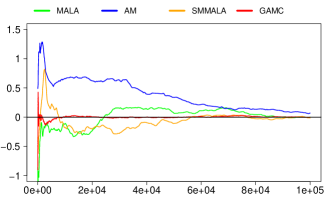
(a)

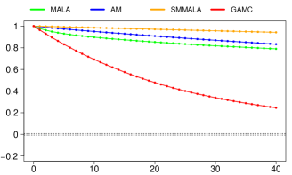
(b)

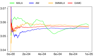
(c)

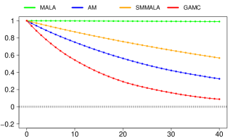
(d)

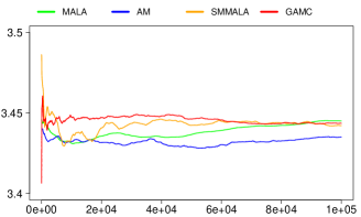
(e)

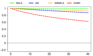
(f)

Figure 1: Overlaid running means as a function of Monte Carlo iteration and overlaid linear autocorrelations of single chains corresponding to one of the twenty, six and eleven parameters of the respective t-distribution, one-planet and two-planet system. The black horizontal line in the t-distribution running mean plot represents the true mode.

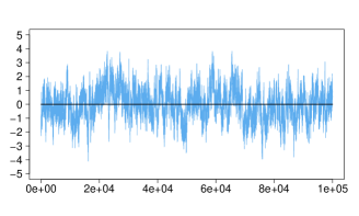
(a)

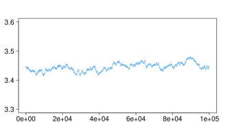
(b)

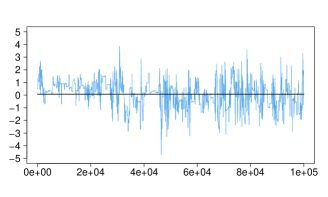
(c)

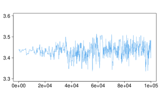
(d)

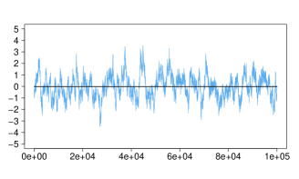
(e)

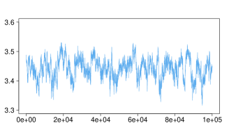
(f)

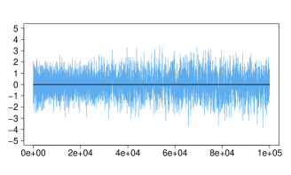
(g)

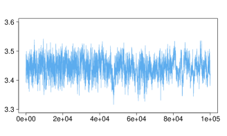
(h)

Figure 2: Trace plots of single chains as a function of Monte Carlo iteration corresponding to one of the twenty and eleven parameters of the respective t-distribution and two-planet system. The same chains were used for generating the trace plots of figure 2 and the associated running means and autocorrelations of figure 1. The black horizontal lines in the t-distribution trace plots represent the true mode.

5.1 Multivariate t-distribution

Monte Carlo samples are drawn from an $n$-dimensional Student-$t$ target $t_{\nu}(0,\frac{\nu-2}{\nu}\Sigma(\xi))$ with $\nu$ degrees of freedom and covariance matrix

$$\Sigma(\xi)=\left(\begin{array}[]{ccccc}1&\xi^{1}&\dots&\xi^{n-2}&\xi^{n-1}\\ \xi^{1}&1&\dots&\xi^{n-3}&\xi^{n-2}\\ \vdots&\vdots&\ddots&\vdots&\vdots\\ \xi^{n-2}&\xi^{n-3}&\dots&1&\xi^{1}\\ \xi^{n-1}&\xi^{n-2}&\dots&\xi^{1}&1\\ \end{array}\right)$$ (19)

for some constant $0<\xi<1$ that determines the level of correlation between parameter coordinates. The elements of the $i$-th diagonal of the $n\cdot n$ covariance matrix $\Sigma(\xi)$ equal $\xi^{i-1},~{}i=1,2,\dots,n$. The scale matrix $\frac{\nu-2}{\nu}\Sigma(\xi)$ of the $t$-distribution scales $\Sigma(\xi)$ by a factor of $\frac{\nu-2}{\nu}$ so that the covariance matrix of the $t$-distribution is $\Sigma(\xi)$.

In this example, the setting is not Bayesian, so there is no prior distribution involved [36]. Instead, MCMC sampling acts as a random number generator to simulate from a $t$-distribution $t_{\nu}(0,\frac{\nu-2}{\nu}\Sigma(\xi))$. The simulated chains are randomly initialized away from the zero mode of the $t$-distribution, and they are expected to converge to zero. In other words, the zero mode of $t_{\nu}(0,\frac{\nu-2}{\nu}\Sigma(\xi))$ is seen as the parameter vector to be estimated.

The dimension of the $t$-target is set to $n=20$, relatively high correlation is induced by selecting $\xi=0.9$ in (19), and some amount of probability mass is maintained in the $t$-distribution tails by choosing $\nu=30$ degrees of freedom. The present example does not reach the realm of a fully-fledged application, especially in terms of log-target complexity, yet it gives a first indication of some common computational costs appearing in more realistic applications, including automatic differentiation and SoftAbs metric evaluations.

Figure 1(a) displays the running means of four chains that correspond to the seventeenth coordinate $\theta_{17}$ of the twenty-dimensional parameter $\theta\sim t_{\nu}(0,\frac{28}{30}\Sigma(0.9))$, with a single chain generated by each of MALA, AM, SMMALA and GAMC. The running mean of the chain simulated using MALA does not appear to converge rapidly to the true mode of zero. This accords with theoretical knowledge. In particular, [43] and [30] have shown that if a target density has tails heavier than exponential or lighter than Gaussian, then a MALA proposal kernel does not yield a geometrically ergodic Markov chain. Furthermore, it can be seen that the chain generated by GAMC converges faster than the chains produced by AM, MALA and SMMALA.

Table 2 reports the minimum, mean, median and maximum ESS of the $n=20$ parameter coordinates. As seen from table 2, GAMC achieves roughly ten times larger ESS in comparison to AM, MALA and SMMALA for the t-distribution example. Figures 1(b), 2(a), 2(c), 2(e) and 2(g) show the autocorrelation and trace plots of the four chains with running means presented by figure 1(a). Figure 1(b) demonstrates that GAMC has the lowest autocorrelation among the four compared samplers. The trace plots provide further circumstantial evidence of the faster mixing of GAMC for the Student-t target. The mixing properties of GAMC in the case of t-distribution come as a surprise, since GAMC was designed to reduce the cost paid for faster mixing rather than to achieve the fastest possible mixing in absolute terms. GAMC has shorter CPU runtime in comparison to SMMALA, but longer runtime than MALA and AM.

With a speed-up of $3.18$, GAMC is about three times more efficient than MALA and orders of magnitude more efficient than AM and SMMALA for the Student-t target $t_{\nu}(0,\frac{28}{30}\Sigma(0.9))$ of this example.

5.2 Radial velocity of a star in planetary systems

The study of exoplanets has emerged as an important area of modern astronomy. While astronomers utilize a variety of different methods for detecting and characterizing the properties of exoplanets and their orbits, each of the prolific methods to date shares several characteristics. First, translating astronomical observations into planet physical and orbital properties requires significant statistical analysis. Second, characterizing planetary systems with multiple planets requires working with high-dimensional parameter spaces. Third, the posterior probability densities are often complex with correlated parameters, non-linear correlations or multiple posterior modes. MCMC has proven invaluable for providing accurate estimates of planet properties and orbital parameters and is now used widely in the field.

For analyzing simple data sets such as one planet detected at high signal-to-noise ratio, the random walk Metropolis-Hastings sampler is effective and the choice of MCMC sampling algorithm is unlikely to be important [10]. For analyzing more complex data sets such as a star with several planets, more care is necessary to avoid poor mixing of the Markov chains. One approach is “artisinal” MCMC, where proposal densities are hand-crafted for a particular problem by making use of physical intuition and validation on simulated data sets [11]. However, it is desirable to identify more sophisticated algorithms that can be efficient with minimal tuning or human intervention. Here, GAMC is applied to simulated radial velocity planet search data sets so as to illustrate the potential of the sampler for future astronomical or other scientific applications.

One prolific method for characterizing the orbits of extrasolar planets is the radial velocity method. Astronomers make a series of precise measurements of the line-of-sight velocity of a target star. The velocity of the star $v(t)$ changes with time $t$ due to the gravitational tug of any planets orbiting it. A basic radial velocity data set consists of a list of $n_{d}$ observation times $t_{i}$, $i=0,1,\dots,n_{d}-1$, and measured velocities $\hat{v}_{i}$.

The observed velocity $\hat{v}_{i}$ of the star at time $t_{i}$ is modelled as the unknown velocity $v(t_{i})$ plus some measurement error $\epsilon_{i}$, as seen in (20). For many planetary systems with $n_{p}$ planets, the stellar line-of-sight velocity $v(t_{i})$ can typically be well approximated by (21). Independent Gaussian measurement errors $\epsilon_{i}$ with variances $\sigma_{i}^{2}$ are assumed according to (22). (20), (21) and (22) introduce the following model for the radial velocity of a star in a planetary system consisting of $n_{p}$ planets:

$$\hat{v}_{i} =v(t_{i})+\epsilon_{i},$$ (20)

$$v(t_{i}) =C\displaystyle\sum_{j=1}^{n_{p}}K_{j}(\cos{(\omega_{j}+T(t_{i},P_{j},e_{j},M_{0,j}))}+e_{j}\cos{(\omega_{j}))},$$ (21)

$$\epsilon_{i} \sim\mathcal{N}(0,\sigma_{i}^{2}).$$ (22)

In (21), $C$ is the systemic line-of-sight velocity of the planetary system, $K_{j}$ is the velocity amplitude induced by the $j$-th planet, $P_{j}$ is the orbital period of the $j$-th planet, $e_{j}$ is the orbital eccentricity of the $j$-th planet, $M_{0,j}$ is the mean anomaly at time $t_{0}=0$ of the $j$-th planet, $\omega_{j}$ is the argument of pericenter of the $j$-th planet, and $T(t_{i},P_{j},e_{j})$ is the true anomaly at time $t_{i}$ of the $j$-th planet.

The true anomaly $T$ is an angle that specifies the location of the planet and star along their orbit at a given time. The true anomaly $T$ is related to the eccentric anomaly $E$ by $\tan(T/2)=\sqrt{\frac{1+e}{1-e}}\tan(E/2)$. The eccentric anomaly $E$ can be calculated from the mean anomaly $M$ from Kepler’s equation, $M=E-E\sin{(E)}$, and an iterative solver. The mean anomaly $M$ increases at a linear rate with time $t$ according to the equation $M(t)=M_{0}+2\pi t/P$.

A parameter vector $(K_{j},P_{j},e_{j},M_{0,j},\omega_{j})$ of length five is associated with the $j$-th planet, as seen from (21). Thus, a total of $n=5n_{p}+1$ model parameters

$$\theta=(C,(K_{1},P_{1},e_{1},M_{0,1},\omega_{1}),\ldots,(K_{n_{p}},P_{n_{p}},e_{n_{p}},M_{0,{n_{p}}},\omega_{n_{p}}))$$

appear in a planetary system with $n_{p}$ planets. The notation $v(t_{i},\theta)$ can be used in place of $v(t_{i})$ to indicate that the stellar line-of-sight velocity (21) of the star depends on the parameters $\theta$.

According to (22), the sum of squares of the normalized measurement errors $\epsilon_{i}/\sigma_{i}$ follow a chi-squared distribution with $n_{d}$ degrees of freedom,

$$\sum_{i=0}^{n_{d}-1}\left(\frac{\epsilon_{i}}{\sigma_{i}}\right)^{2}\sim\chi_{n_{d}}^{2}.$$ (23)

The log-likelihood arises from (23) and (20) as

$$\mathcal{L}(t,\hat{v},\sigma|\theta)=-\frac{1}{2}\sum_{i=0}^{n_{d}-1}\left(\frac{v(t_{i},\theta)-\hat{v}_{i}}{\sigma_{i}}\right)^{2},$$ (24)

where $t=(t_{0},t_{1},\dots,t_{n_{d}-1})$, $\hat{v}=(\hat{v}_{0},\hat{v}_{1},\dots,\hat{v}_{n_{d}-1})$, $\sigma=(\sigma_{0},\sigma_{1},\dots,\sigma_{n_{d}-1})$. It is assumed that the measurement uncertainties $\sigma$ are known, so $t$, $\hat{v}$ and $\sigma$ make up the available data.

For the relatively simple model described by (24) and (21), astronomers commonly use a set of priors elicited during a 2013 SAMSI program on astrostatistics. Modified Jeffreys priors are adopted for the velocity amplitudes $K_{j}$ and orbital periods $P_{j}$. Uniform priors are employed for the orbital eccentricities $e_{j}$, velocity offsets $M_{0,j}$ and angle offsets $\omega_{j}$ according to $e_{j}\sim\mathcal{U}[0,1)$, $\omega_{j}\sim\mathcal{U}[0,2\pi)$, $M_{0,j}\sim\mathcal{U}[0,2\pi)$.

GAMC is benchmarked on two simulated data sets, of which one consists of $n_{p}=1$ planet and the other one comprises $n_{p}=2$ planets. In each case, $n_{d}=50$ observed velocities $\hat{v}\in\mathbb{R}^{50}$ are simulated at time points $t\in\mathbb{R}^{50}$ spread uniformly over two years.

5.2.1 One-planet system

For the one-planet system, the isochronal velocities $\hat{v}_{i}$ are simulated using $C=1.0$, $K_{1}=20m/s$, $P_{1}=50$ days, $e_{1}=0.2$, $M_{0,1}=\pi/4$, $\omega_{1}=\pi/4$ and $\sigma_{i}=2m/s$ for $i=0,1,\dots,49$. The parameter vector for this one-planet system is

$$\theta=(C,K_{1},P_{1},e_{1},M_{0,1},\omega_{1}),$$

so $n=6$ parameters are simulated from the target built upon log-likelihood (24).

Figure 1(c) shows the running means of four chains for the velocity amplitude $K_{1}$ induced by the single planet, with one chain generated by each of the four compared samplers. SMMALA and GAMC seem to converge to the same value, although the latter appears to converge faster.

Table 2 provides the minimum, mean, median and maximum ESS of the $n=6$ astronomical parameters $\theta=(C,K_{1},P_{1},e_{1},M_{0,1},\omega_{1})$. As seen from table 2 and figure 1(d), GAMC exhibits the largest ESS and smallest autocorrelation and therefore appears to have the fastest mixing. In terms of CPU runtime, GAMC is about three times faster than SMMALA, but slower than MALA and AM.

Apart from attaining the fastest mixing, GAMC outperforms MALA by a factor of $246.59$ in terms of speed-up and SMMALA by a factor of even higher order of magnitude. GAMC has the second-best efficiency, with AM being the most efficient by reaching a $378.50$ speed-up in comparison to MALA. The higher efficiency of AM over GAMC for this example is attributed to the relatively small dimension $n=6$ of the parameter space. GAMC might still be preferred over AM for this low-dimensional one-planet system, considering that the former sampler has higher ESS and higher acceptance rate than the latter at a relatively modest additional computational cost.

5.2.2 Two-planet system

For the two-planet system, the isochronal velocities $\hat{v}_{i}$ are simulated using $C=1.0$, $K_{1}=30m/s$, $P_{1}=40$ days, $e_{1}=0.2$, $M_{0,1}=\pi/4$, $\omega_{1}=\pi/4$, $K_{2}=30m/s$, $P_{2}=80.8$ days, $e_{2}=0.2$, $M_{0,2}=\pi/4$, $\omega_{2}=\pi/4$, and $\sigma_{i}=2m/s$ for $i=0,1,\dots,49$. The parameter vector

$$\theta=(C,K_{1},P_{1},e_{1},M_{0,1},\omega_{1},K_{2},P_{2},e_{2},M_{0,2},\omega_{2})$$

is associated with this two-planet system, so $n=11$ parameters are simulated from the target built upon log-likelihood (24).

Figure 1(e) displays the running means of four chains for the velocity amplitude $K_{1}$ induced by planet one of the two-planet system, with one chain generated by each of the four compared samplers. GAMC seems to converge the fastest, followed by SMMALA. AM does not show signs of convergence, which is related to the low acceptance rate of AM in this example.

Table 2 provides the minimum, mean, median and maximum ESS of the eleven parameters. Similarly to the one-planet system, GAMC attains the highest ESS, lowest autocorrelation and most rapidly mixing trace in the case of the two-planet system, as seen from table 2 and figures 1(f), 2(b), 2(d), 2(f) and 2(h).

The MALA trace plot of figure 2(b) is characterized by slow exploration of the state space of parameter $K_{1}$, which is attributed to the small stepsize required for maintaining an acceptance rate close to the optimal rate of $57.4\%$. Although the AM chain of figure 2(d) takes longer proposal steps than its MALA counterpart, AM has a very low acceptance rate of $0.01\%$. SMMALA offers a substantial improvement in mixing over MALA and AM according to figure 2(f), while GAMC appears to have the most rapid mixing among the four samplers (figure 2(h)).

GAMC ranks third in absolute runtime behind AM and MALA for the system of two planets (table 2). However, AM does not work in the case of two planets, since it fails to converge and it has a prohibitively low acceptance rate of $0.01\%$. Besides, MALA does not seem to converge either and it explores the state space very slowly. In fact, the superiority of GAMC in this example is depicted by the largest ESS and highest overall efficiency, with a relative speed-up about $25$ and $20$ times higher than MALA and SMMALA, respectively.

5.3 Synopsis of empirical results from simulations

GAMC has the highest ESS and thus the fastest mixing in all three examples. This empirical finding might indicate that some random proposal kernels or combinations of proposal kernels have better mixing properties than proposal mechanisms based on solitary geometric kernels.

In the two most computationally demanding examples (t-distribution and two-planet system), GAMC manifested its capacity to achieve the highest speed-up among its competing samplers. Thus, combining kernels might help achieve high mixing per step with low computational cost per step for a range of expensive models.

Simulations have led empirically to an optimal acceptance rate between $20\%$ and $40\%$ for GAMC. This might be explained by the fact that AM contributes the majority of Monte Carlo steps to GAMC for relatively small values of the tuning parameter $r$ in (15).

6 Discussion

This paper initiates a conceptually straightforward, yet potentially powerful, approach to the problem of making manifold MCMC algorithms more computationally accessible. The main idea is to combine geometric and non-geometric proposal kernels to find a balance between computational cost and fast mixing. GAMC has been empirically validated on a t-distribution and on astronomical models of planetary systems. The initial simulation studies of this paper, along with applications of GAMC on exoplanet transit timing variation models in [47], reveal the potential of GAMC in terms of sampling efficiency relative to algorithms such as SMMALA.

MCMC algorithms that exploit geometric information about the posterior shape are likely to be more efficient in terms of the absolute number of model evaluations. Manifold MCMC methods could make it practical to generate posterior samples with increased effective sample sizes. Unfortunately, computing partial derivatives for every proposal, as required for MMALA or SMMALA, would be extremely expensive.

GAMC algorithms have the potential to significantly reduce the number of gradient and Hessian evaluations, and are thus expected to accelerate computations by over an order of magnitude relative to SMMALA for expensive models. Exploring ways of injecting local geometric information in adaptive or other non-geometric MCMC methods promises to make manifold MCMC more amenable to realistic applications. GAMC opens up possible avenues of methodological research for building proposal mechanisms based on random proposal kernels.

References

- [1] C. Andrieu and E. Moulines, On the ergodicity properties of some adaptive MCMC algorithms, The Annals of Applied Probability, 16 (2006), 1462–1505.
- [2] Y. Bai, G. O. Roberts and J. S. Rosenthal, On the containment condition for adaptive Markov chain Monte Carlo algorithms, Advances and Applications in Statistics, 21.
- [3] M. Betancourt, A general metric for Riemannian manifold Hamiltonian Monte Carlo, in Proceedings of 1s international conference on Geometric Science of Information (eds. F. Nielsen and F. Barbaresco), Springer, Berlin Heidelberg, 2013, 327–334.
- [4] B. Calderhead, M. Epstein, L. Sivilotti and M. Girolami, Bayesian approaches for mechanistic ion channel modeling, in In silico systems biology (ed. V. M. Schneider), Humana Press, Totowa, NJ, 2013, chapter 13, 247–272.
- [5] B. Calderhead and M. Girolami, Statistical analysis of nonlinear dynamical systems using differential geometric sampling methods, Interface Focus, 1.
- [6] S. Chib and E. Greenberg, Understanding the Metropolis-Hastings algorithm, The American Statistician, 49 (1995), 327–335.
- [7] U. Şimşekli, R. Badeau, A. T. Cemgil and G. Richard, Stochastic quasi-Newton Langevin Monte Carlo, in Proceedings of the 33rd International Conference on Machine Learning (eds. M. F. Balcan and K. Q. Weinberger), Proceedings of Machine Learning Research, 2016, 642–651.
- [8] S. Davie and A. J. Stothers, Improved bound for complexity of matrix multiplication, Proceedings of the Royal Society of Edinburgh, Section: A Mathematics, 143 (2013), 351–369.
- [9] S. Duane, A. Kennedy, B. J. Pendleton and D. Roweth, Hybrid Monte Carlo, Physics Letters B, 195 (1987), 216–222.
- [10] E. B. Ford, Quantifying the uncertainty in the orbits of extrasolar planets, The Astronomical Journal, 129 (2005), 1706–1717.
- [11] E. B. Ford, Improving the efficiency of Markov chain Monte Carlo for analyzing the orbits of extrasolar planets, The Astrophysical Journal, 642 (2006), 505–522.
- [12] F. L. Gall, Powers of tensors and fast matrix multiplication, in Proceedings of the 39th international symposium on symbolic and algebraic computation, Association for Computing Machinery, 2014, 296–303.
- [13] C. J. Geyer, Practical Markov chain Monte Carlo, Statistical Science, 7 (1992), 473–483.
- [14] P. E. Gill, G. H. Golub, W. Murray and M. A. Saunders, Methods for modifying matrix factorizations, Mathematics of Computation, 28 (1974), 505–535.
- [15] M. Girolami and B. Calderhead, Riemann manifold Langevin and Hamiltonian Monte Carlo methods, Journal of the Royal Statistical Society: Series B (Statistical Methodology), 73 (2011), 123–214.
- [16] A. Griewank, On automatic differentiation and algorithmic linearization, Pesquisa Operacional, 34 (2014), 621–645.
- [17] A. Griewank and A. Walther, Evaluating derivatives: principles and techniques of algorithmic differentiation, 2nd edition, no. 105 in Other Titles in Applied Mathematics, SIAM, Philadelphia, PA, 2008.
- [18] J. E. Griffin and S. G. Walker, On adaptive Metropolis-Hastings methods, Statistics and Computing, 23 (2013), 123–134.
- [19] H. Haario, M. Laine, A. Mira and E. Saksman, DRAM: efficient adaptive MCMC, Statistics and Computing, 16 (2006), 339–354.
- [20] H. Haario, E. Saksman and J. Tamminen, An adaptive Metropolis algorithm, Bernoulli, 7 (2001), 223–242.
- [21] B. Hajek, Cooling schedules for optimal annealing, in Open problems in communication and computation (eds. T. M. Cover and B. Gopinath), Springer New York, New York, NY, 1987, 147–150.
- [22] N. J. Higham, Computing a nearest symmetric positive semidefinite matrix, Linear Algebra and its Applications, 103 (1988), 103–118.
- [23] N. J. Higham, Computing the nearest correlation matrix - a problem from finance, IMA Journal of Numerical Analysis, 22 (2002), 329–343.
- [24] N. J. Higham and N. Strabić, Anderson acceleration of the alternating projections method for computing the nearest correlation matrix, Numerical Algorithms, 72 (2016), 1021–1042.
- [25] T. House, Hessian corrections to the Metropolis adjusted Langevin algorithm, arXiv.
- [26] O. Kallenberg, Random measures, theory and applications, Springer, 2017.
- [27] S. Kirkpatrick, C. D. Gelatt and M. P. Vecchi, Optimization by simulated annealing, Science, 220 (1983), 671–680.
- [28] T. S. Kleppe, Adaptive step size selection for Hessian-based manifold Langevin samplers, Scandinavian Journal of Statistics, 43 (2016), 788–805.
- [29] S. Lan, T. Bui-Thanh, M. Christie and M. Girolami, Emulation of higher-order tensors in manifold Monte Carlo methods for Bayesian inverse problems, Journal of Computational Physics, 308 (2016), 81–101.
- [30] S. Livingstone and M. Girolami, Information-geometric Markov chain Monte Carlo methods using diffusions, Entropy, 16 (2014), 3074.
- [31] M. Locatelli, Simulated annealing algorithms for continuous global optimization: convergence conditions, Journal of Optimization Theory and Applications, 104 (2000), 121–133.
- [32] J. F. D. Martin and J. M. R. no Sierra, A comparison of cooling schedules for simulated annealing, Encyclopedia of Artificial Intelligence, 344–352.
- [33] R. M. Neal, Bayesian learning for neural networks, vol. 118, Springer, 1996.
- [34] J. Neveu, Mathematical foundations of the calculus of probability, Holden-Day, Inc, 1965.
- [35] Y. Nourani and B. Andresen, A comparison of simulated annealing cooling strategies, Journal of Physics A: Mathematical and General, 31 (1998), 8373–8385.
- [36] T. Papamarkou, A. Mira and M. Girolami, Monte Carlo methods and zero variance principle, in Current trends in Bayesian methodology with applications (eds. S. K. Upadhyay, U. Singh, D. K. Dey and A. Loganathan), Chapman and Hall/CRC, 2015, chapter 22, 457–476.
- [37] M. Pereyra, Proximal Markov chain Monte Carlo algorithms, Statistics and Computing, 26 (2016), 745–760.
- [38] J. Revels, M. Lubin and T. Papamarkou, Forward-mode automatic differentiation in julia, arXiv.
- [39] G. O. Roberts and J. S. Rosenthal, Optimal scaling of discrete approximations to Langevin diffusions, Journal of the Royal Statistical Society: Series B (Statistical Methodology), 60 (1998), 255–268.
- [40] G. O. Roberts and J. S. Rosenthal, Coupling and ergodicity of adaptive Markov chain Monte Carlo algorithms, Journal of Applied Probability, 44 (2007), 458–475.
- [41] G. O. Roberts and J. S. Rosenthal, Examples of adaptive MCMC, Journal of Computational and Graphical Statistics, 18 (2009), 349–367.
- [42] G. O. Roberts and O. Stramer, Langevin diffusions and Metropolis-Hastings algorithms, Methodology And Computing In Applied Probability, 4 (2002), 337–357.
- [43] G. O. Roberts and R. L. Tweedie, Exponential convergence of Langevin distributions and their discrete approximations, Bernoulli, 2 (1996), 341–363.
- [44] E. Saksman and M. Vihola, On the ergodicity of the adaptive Metropolis algorithm on unbounded domains, The Annals of Applied Probability, 20 (2010), 2178–2203.
- [45] R. Schwentner, T. Papamarkou, M. O. Kauer, V. Stathopoulos, F. Yang, S. Bilke, P. S. Meltzer, M. Girolami and H. Kovar, EWS-FLI1 employs an E2F switch to drive target gene expression, Nucleic Acids Research.
- [46] M. Seeger, Low rank updates for the Cholesky decomposition, Technical report, University of California, Berkeley, 2004.
- [47] N. W. Tuchow, E. B. Ford, T. Papamarkou and A. Lindo, The efficiency of geometric samplers for exoplanet transit timing variation models, Monthly Notices of the Royal Astronomical Society, 484 (2019), 3772–3784.
- [48] M. Vihola, Robust adaptive Metropolis algorithm with coerced acceptance rate, Statistics and Computing, 22 (2012), 997–1008.
- [49] J. H. Wilkinson, Modern error analysis, SIAM Review, 13 (1971), 548–568.
- [50] V. V. Williams, Breaking the Coppersmith-Winograd barrier, 2011.
- [51] T. Xifara, C. Sherlock, S. Livingstone, S. Byrne and M. Girolami, Langevin diffusions and the Metropolis-adjusted Langevin algorithm, Statistics and Probability Letters, 91 (2014), 14–19.