Solid-on-solid single block dynamics under mechanical vibration

Abstract

The suppression of friction between sliding objects, modulated or enhanced by mechanical vibrations, is well established. However, the precise conditions of occurrence of these phenomena is not well understood. Here we address these questions focusing on a simple spring–block model, which is relevant to investigate friction both at the atomistic as well as the macroscopic scale. This allows to investigate the influence on friction of the properties of the external drive, of the geometry of the surfaces over which the block moves, and of the confining force. Via numerical simulations and a theoretical study of the equations of motion we identify the conditions under which friction is suppressed and/or recovered, and evidence the critical role played by surface modulations and by the properties of the confining force.

I Introduction

The frictional force between sliding surfaces is affected by suitable mechanical vibrations, which may facilitate or inhibit their relative motion and the associated stick–slip dynamics heuberger ; rozman ; gao ; capozza2009 . This effect occurs both at the atomistic as well as at the macroscopic scale, as the physics responsible for friction is expected to be largely the same urbakh . Indeed, at the nanoscale vibrations have been experimentally observed to play a relevant role urbakh ; gao ; brace ; diete72 ; capozza2009 ; socoliuc2006 , and are relevant for the design of microscopic devices. Likewise, at the mesoscopic scale numerical aharonov and experimental nasuno ; tsai ; daltonpre2002 ; johnson2005 ; johnson2008 works showed that external perturbations may affect the frictional forces of sheared particulate systems. These results are frequently connected to the geophysical scale scholz72 ; diete79 ; ruina83 where it is possible that earthquakes, a stick–slip frictional instability marone98 ; helmstetter , may be actually triggered by incoming seismic waves Stacey , acting as perturbations. This phenomenon is regularly observed in numerical simulations of seismic fault models PRL2010 ; Griffa .

The reduction of friction due to vibrations can be easily attributed to the induced separation of the sliding surfaces. Accordingly, it is surprising that an increase of the vibrational intensity may also lead to a recovery of the friction coefficient, a phenomenon observed in systems of sheared and vibrated Lennard-Jones particles at zero temperature capozza2009 . In particular, Ref. capozza2009 identified a range of frequencies where friction is suppressed, and related this range to the amplitude of oscillation as well as to the system inertia and damping constant. The decrease of the friction coefficient in sheared particulate systems is qualitatively analogous to the decrease of the viscosity of sheared particulate suspensions, which is known to occur when particles order in planes parallel to the shearing direction tsai . Accordingly, one may suspect that the presence of particles in between the sliding surfaces is essential to reproduce friction suppression and recovery, a question which has not yet been clarified. In addition, the influence of the geometry of the oscillating surface on the effective friction coefficient has not been explicitly investigated. This is an important point, considering that surfaces of macroscopic objects are expected to be rough, while atomistic surfaces are isopotential surfaces, and have a periodicity dictated by the underlying lattice structure.

Here we address these questions via the theoretical and numerical study of three variants of a simple solid–on–solid model, where a block is pulled horizontally by a spring driven at constant velocity. In all cases the block moves along a surface which is vibrated along the vertical direction, and the role of both the amplitude and the frequency of vibration is explored. In model A the surface is flat and the confining stress is vertical; in model B the surface is sinusoidal and the confining stress is vertical; in model C the surface is sinusoidal and the confining stress is normal to the surface.

In the absence of vibrations, spring block models are characterized by a sliding (fluid) phase, and by a stick–slip (solid) phase, and the transition between the two can be analytically obtained Vasconcelos . In the presence of vibrations, these two phases occur in different regions of the vibrational amplitude/vibrational frequency diagram, and depend on model details. In particular, model B results not to be influenced by the vibrations, and its behavior only depends on the driving velocity. Conversely, in models A and C we find the expected transition from the stick-slip to the sliding phase for increasing frequency (or amplitude) of the oscillating plate. This transition occurs when the maximum acceleration of the oscillating plate overcomes gravity (or $P_{l}/m$ in model C, $P_{l}$ being the confining force). This is the only transition observed in model A.

In model C, a further increase of the frequency leads to a second transition whereby the system re–enters the stick–slip phase, analogously to what observed in Ref. capozza2009 . This second transition originates from a balance between dissipative and inertial forces.

The paper is organized as follows: Section II introduces the equations of motion of the three spring–block models, and the order parameter used to study the dynamical properties of the system; Section III reports on results of numerical simulations obtained by changing the control parameters; different dynamical behaviors are discussed and demonstrated through theoretical analysis; conclusions and open questions are outlined in Section IV.

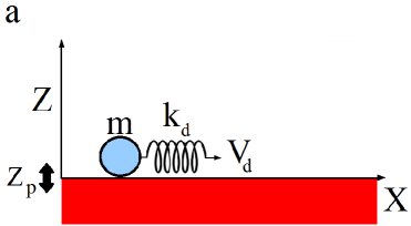
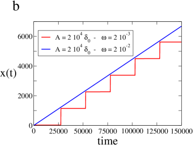
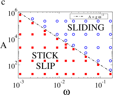
Figure 1: (color online) a) Schematic representation of model A: a point–particle is driven via an elastic spring on an oscillating flat plane. b) Time dependence of the horizontal position $x(t)$ of the block for two different oscillation frequencies $\omega$ of the plate, at fixed oscillation amplitude $A$, in the sick–slip and in the sliding phase. c) Phase diagram of model A. The symbols indicate the different phases of the system and are located in positions defined by the values of the parameters $A$ and $\omega$ used in the simulations. A transition from the stick–slip (squares) to the sliding (circles) phase occurs on increasing $A$ or $\omega$. The transition line (dotted line) is given by $A=g\omega_{1}^{-2}$.

II Single block dynamic

II.1 Models

We have investigated three variants of the usual spring–block model, where a point particle of mass $m$ is driven via a spring of elastic constant $k_{d}$ on a substrate. One extremity of the driving spring is attached to the block, while the other moves with an imposed driving velocity $V_{d}$. The block is considered as a point-like body and interacts with an oscillating plate (see Fig. 1a) through contact forces which give rise to a viscoelastic response.

We denote with $x$ and $z$ the horizontal and vertical positions of the block, respectively, and with $Z_{p}$ the vertical position of the top surface of the plate. This varies in space and time as $Z_{p}(x,t)=A\sin(\omega t)+A_{x}\sin(\omega_{x}x)$, $(A,\omega)$ and $(A_{x},\omega_{x})$ fixing its temporal and spatial oscillations.

In model A, $A_{x}=0$, and the equations of motion along the two directions with respect to a fixed reference system are given by:

$$m\ddot{z}=k_{n}(Z_{p}-z)\Theta(Z_{p}-z)-\gamma_{n}(\dot{z}-\dot{Z_{p}})\Theta(Z_{p}-z)-mg$$ (1)

$$m\ddot{x}=-k_{d}(x-V_{\textrm{d}}t)-\gamma_{t}\dot{x}-k_{t}\mathcal{F}(\dot{x},Z_{p}-z)$$ (2)

where $\Theta$ is the Heaviside step function, $g$ is the gravity, $k_{n,t}$ and $\gamma_{n,t}$ are the elastic and the damping constants respectively, $k_{d}$ is the elastic constant of the external drive. The quantity $k_{t}\mathcal{F}(\dot{x})$ is a frictional term which is only present when the plate and the block are in contact, and this introduces a coupling between the two equations. In particular, following a standard procedure to implement an history dependent friction between sheared macroscopic surfaces materials , we assume this term to be proportional to the shear displacement over the lifetime of the contact, which depends on the vertical motion. If, during the time interval $t$–$t_{0}$, the block is in contact with the plate, then the friction term is given by $\mathcal{F}(\dot{x}(t),Z_{p}-z)=\int_{t_{0}}^{t}\dot{x}(t^{\prime})dt^{\prime}$. The friction term $\mathcal{F}$ is set to zero as soon as the block detaches from the plate. The Coulomb friction is taken into account through the condition $|k_{t}\mathcal{F}|<\mu_{s}N$, where $N$ is the resultant of the normal forces and $\mu_{s}$ is the coefficient of static friction. When the Coulomb condition is violated $\mathcal{F}$ is set to zero.

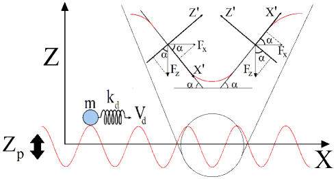
Figure 2: (color online) Models B and C: motion on a plate with a horizontal periodic corrugation. As for the model A, the block is considered as a point-like body interacting with the corrugated plate via contact forces. The magnification shows the reference frame used to study the dynamics of the block. In this frame each force has a vertical and a horizontal component which depends on the angle $\alpha=\arctan\left(\frac{\partial{Z_{p}}}{\partial{x}}\right)$.

In the model B, $A_{x}>0$. In this case it is convenient to write the equations of motion in a frame of reference which moves along with the plate, with the horizontal axis tangential to the plate, see Fig. 2. In this frame the equations of motion are

$$m\ddot{z}^{\prime} = k_{n}(Z_{p}^{\prime}-z^{\prime})\Theta(Z_{p}^{\prime}-z^{\prime})-\gamma_{n}(\dot{z}^{\prime}-\dot{Z_{p}^{\prime}})\Theta(Z_{p}^{\prime}-z^{\prime})+$$ (3)

$$+ k_{d}(x^{\prime}-V_{\textrm{d}}t)\sin(\alpha)-mg\cos(\alpha)$$

$$m\ddot{x}^{\prime} = -k_{d}(x^{\prime}-V_{\textrm{d}}t)\cos(\alpha)-\gamma_{t}\dot{x}^{\prime}-k_{t}\cdot\mathcal{F}(\dot{x}^{\prime},Z^{\prime}_{p}-z^{\prime})-$$ (4)

$$- mg\sin(\alpha),$$

where $\alpha=\arctan\left(\frac{\partial{Z_{p}}}{\partial{x}}\right)$ at fixed time. In the case of friction at atomic level, the periodic corrugation models the atomic lattice capozza2009 whereas, in the case of seismic fault, corrugation represents seismic asperities asperities .

In the model C, we consider the possibility that the mass is not subject to the gravity, but to a confining force $P_{l}$ which is always perpendicular to the surface. This is expected to occur in the atomistic systems, when the block slides over a series of particles periodically arranged on a line, and interacts with them via Lennard–Jones like potentials, as described in Sec. III C. In this case, the equations of motion are

$$m\ddot{z}^{\prime} = k_{n}(Z_{p}^{\prime}-z^{\prime})\Theta(Z_{p}^{\prime}-z^{\prime})-\gamma_{n}(\dot{z}^{\prime}-\dot{Z_{p}^{\prime}})\Theta(Z_{p}^{\prime}-z^{\prime})+$$ (5)

$$+ k_{d}(x^{\prime}-V_{\textrm{d}}t)\sin(\alpha)-P_{l}$$

and

$$m\ddot{x}^{\prime} = -k_{d}(x^{\prime}-V_{\textrm{d}}t)\cos(\alpha)-\gamma_{t}\dot{x}^{\prime}-k_{t}\mathcal{F}(\dot{x}^{\prime},Z^{\prime}_{p}-z^{\prime}).\;\quad$$ (6)

II.2 Order parameter

To differentiate the stick–slip and the flowing phases we introduce an order parameter, defined as

$$\phi=\frac{\langle(\dot{x}-V_{d})^{2}\rangle_{t_{a}}}{V_{d}^{2}}$$ (7)

where the brackets indicate temporal averages over a period $t_{a}$. In the flowing phase, the block moves with the external drive velocity ($\dot{x}=V_{d}$) and therefore $\phi=0$. Conversely, in the stick-slip phase, $\phi$ takes a finite value that depends on the period $t_{a}$ (or the number of occurred slips during $t_{a}$). Indeed, the temporal average in the stick–slip phase includes long stick times with practically zero block velocity, and short slip intervals with very high block velocity. Therefore, the values of $\phi>0$ allow to easily identify the stick-slip phase.

II.3 Units and numerical details

In the following we present results obtained by solving via a first order numerical integration the differential equations (1)-(6). In the simulations, we have monitored the horizontal and vertical positions of the block as a function of the control parameters of the plate, $A$ and $\omega$, while keeping the values of the other parameters fixed to the typical values used in molecular dynamics simulations materials . We choose as numerical units $m=1$, $g=1$ and $k_{n}=1$. This corresponds to express lengths in units of $\delta_{0}=mg/k_{n}$, i.e. the rest position of the block inside the plate in the absence of oscillations, and times in units of $\tau_{0}=\sqrt{m/k_{n}}$. The other parameters are fixed to the values $k_{t}=0.28$, $\gamma_{n}=7\cdot 10^{-2}$, $\gamma_{t}=2.5\cdot 10^{-4}$, $\mu_{s}=0.5$, $k_{d}=5\cdot 10^{-4}$ and $V_{d}=2\cdot 10^{-5}$, unless otherwise specified. The integration time step of the equations of motion is $4\cdot 10^{-4}$. In our simulations the chosen parameters assure a quasi-static regime ($V_{d}\simeq 0$) and stick-slip motion in the limit of no external oscillations ($A=0$, $\omega=0$). Whereas the details of the dynamics depend on the values of these parameters, the main results presented below are very robust to changes of the parameters and the physical properties of the system remain unaltered.

III Results

III.1 Model A 

The dynamics in the vertical direction of model A are conveniently investigated in a frame of reference oscillating with the plate, making the change of variable $y=z-Z_{p}$. In this frame of reference Eq. (1) takes the form

$$m\ddot{y}=-k_{n}y\Theta(-y)-\gamma_{n}\dot{y}\Theta(-y)-mg+m\ddot{Z_{p}}.$$

We first study the case of a constant perturbation $\ddot{Z_{p}}=0$. In this case the above equation has an equilibrium solution $y=-mg/k_{n}$ indicating that the block is always in contact with the plate at a fixed penetration depth. Eq. (2) presents a stationary solution, $k_{t}V_{S}=k_{d}(V_{d}-V_{S})$, when the block moves with a constant velocity $V_{S}=V_{d}k_{d}/(k_{t}+k_{d})$. In this case the friction term $\mathcal{F}$ grows linearly in time, $\mathcal{F}=V_{S}(t-t_{0})$. As soon as $\mathcal{F}$ reaches the Coulomb threshold value $\mu_{s}mg$, the block is no longer stable and a slip starts. The slip ends when the whole elastic energy of the driving spring is relaxed ($x=V_{d}t$). Accordingly when $V_{S}\ll V_{d}$ one observes regular stick-slip. The duration $t_{stick}$ of the stick phase can be obtained from $k_{t}V_{S}t_{stick}=\mu_{s}mg$, while the length of each slip is given by $\Delta x_{slip}=\frac{\mu_{s}mg}{k_{t}V_{s}}(V_{d}-V_{S})=\mu_{s}mg/k_{d}$.

We now consider the effect of the external perturbation, $\ddot{Z_{p}}\neq 0$, distinguishing two cases. When $\ddot{Z_{p}}$ is always smaller than $g$, then the block is confined within the plate, and the dynamics along the $x$ direction are exactly the ones described when $A=0$. Also the slip length and stick duration are independent of the perturbation parameters $A$ and $\omega$. On the other hand, as soon as $\ddot{Z_{p}}>g$, i.e. $A\omega_{1}^{2}>g$, the block undergoes a vertical positive acceleration, detaches from the plate and accelerates also in the horizontal direction, aiming to reach the velocity of the external drive, $\dot{x}(t)=V_{d}$ (Fig. 1b). In this case, the dynamics along $z$ consist of a series of jumps over the plate. In the range of parameters we have explored the duration of the contact interval, of order $\sqrt{m/k_{n}}$, is much smaller than the time of flight, $2A\omega/g$. As a consequence, the friction term $\mathcal{F}$ is always negligible and the block follows the external drive.

Summarizing, in model A by systematically changing the control parameters we find two different dynamical regimes, stick–slip and sliding, separated by a dynamic transition occurring when $A=g\omega_{1}^{-2}$, as illustrated in Fig. 1c. This friction–suppression transition is the only one we observe in this model.

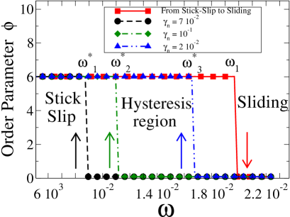
Figure 3: (color online) Evolution of the order parameter $\phi$ during a frequency cycle performed with model A. At fixed amplitude we quasi-statically increase the frequency until the system transients to the sliding phase at a frequency $\omega_{1}$ (squares), which does not depend on $\gamma_{n}$. The order parameter drops to zero at $\omega_{1}$. On the contrary, the reverse transition from the sliding to the stick–slip phase on decreasing the frequency occurs at a $\gamma_{n}$ dependent frequency $\omega^{*}$. $\omega^{*}$ approaches $\omega_{1}$ on increasing $\gamma_{n}$, as illustrated.

The transition from the stick–slip to the sliding phase is characterized by an hysteresis region, whose extension depends on the damping parameter $\gamma_{n}$, as illustrated in Fig. 3. Precisely, the transition from the stick-slip to the sliding phase always occurs at the same frequency $\omega_{1}$, while the reverse transition occurs at a $\gamma_{n}$ dependent frequency $\omega^{*}(\gamma_{n})$. On increasing $\gamma_{n}$, $\omega^{*}(\gamma_{n})$ approaches $\omega_{1}$, and the hysteresis disappears. An analogous hysteresis effect is observed when the transition is crossed by varying the amplitude of the perturbation. The origin of this phenomenon is simply related to an excess of energy accumulated in the sliding phase. A similar phenomenon occurs in magnetic systems risken and frictionless granular systems jammzero .

III.2 Model B

We now consider how a periodic modulation of the oscillating surface influences the dynamics of the system. To this end we fix $A_{x}=10^{3}$ and $\omega_{x}=2\cdot 10^{-2}$, and consider an external drive with $V_{d}=2\cdot 10^{-4}$ and $k_{d}=5\cdot 10^{-6}$. Considering that, in the stick phase, the system is in a steady-state position $x^{*}$ with $\dot{x}(t)=\ddot{x}(t)=0$. We start by identifying the steady-state solutions of Eq. (4), and to this end we neglect the history dependent frictional term by setting $k_{t}=0$. The equation for the positions $x^{*}$ is

$$-k_{d}(x^{*}-V_{\textrm{d}}t)\cos(\alpha)-mg\sin(\alpha)=0$$ (8)

which, combined with the definition of $\alpha$, leads to:

$$\cos(\omega_{x}x^{*})=K(x^{*}-V_{\textrm{d}}t)\quad\textrm{with}\quad K=\frac{-k_{d}}{A_{x}\omega_{x}mg}.$$ (9)

Given the values of $K$ and $V_{d}$, this equation has several solutions as a function of time. This is illustrated in Fig. 4, where we show the solutions of Eq. (9) at three different times $t_{3}>t_{2}>t_{1}$, indicating with filled squares the stable solutions, and with open circles the unstable ones.

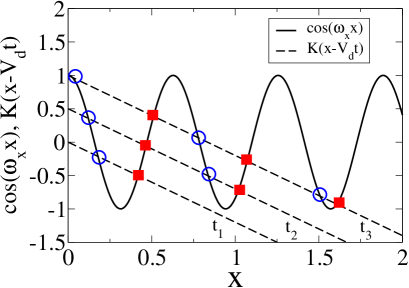
Figure 4: (color online) Graphical solution of Eq. (9). Given the values of $K_{d}$ and $V_{d}$, several solutions may exist as a function of time. In the figure, $t_{3}>t_{2}>t_{1}$. If the solution is located on the side of the cosine function with positive slope, then the steady-state position is stable (squares) and the block is stuck. Conversely, the other solutions (circles) are unstable.

If the system is in a stable solution, then as time increases its position drifts with a velocity $V_{\textrm{stick}}\left(x^{*}(t)\right)$ to different stable positions, until it enters an unstable solution and starts flowing. The drift velocity $V_{\textrm{stick}}\left(x^{*}(t)\right)$ can be estimated considering the response to small perturbations around the steady-state position, i.e. $(x^{*},t)\rightarrow(x^{*}+dx,t+dt)$. Indeed, from Eq. (9) we have

$$\cos(\omega_{x}(x^{*}+dx))=K(x^{*}+dx-V_{\textrm{d}}t-V_{\textrm{d}}dt),$$

whose first order expansion leads to

$$\cos(\omega_{x}x^{*})-\omega_{x}\sin(\omega_{x}x^{*})dx=K(x^{*}+dx-V_{\textrm{d}}t-V_{\textrm{d}}dt).$$

The drift velocity is therefore given by

$$V_{\textrm{stick}}(x^{*})=\left.\frac{dx}{dt}\right|_{x=x^{*}}=\frac{V_{d}}{1-\frac{mgA_{x}\omega_{x}^{2}}{k_{d}}\sin({\omega_{x}x^{*}})}.$$ (10)

From Eq. (9) the stable solutions correspond to $\sin({\omega_{x}x^{*}})<0$ and in particular, for the investigated parameters $\sin(\omega_{x}x^{*})\simeq-1$ and $k_{d}/mgA_{x}\omega_{x}^{2}\gg 1$. As a consequence we have $V_{\textrm{stick}}\ll V_{d}\ll 1$ and this velocity is negligible.

When $\cos(\omega_{x}x^{*})$ reaches $1$, the subsequent closest solution of Eq. (9) is no longer stable, and the system starts flowing. Depending on the stored elastic energy $k_{d}(x(t)-V_{d}t)^{2}$, one may observe a large slip ($\Delta x^{*}\ll\omega_{x}^{-1}$), or a transition to the sliding phase. Accordingly, the horizontal dynamics of model B are surprisingly unaffected by the oscillating perturbation, and the two regimes are only fixed by the value of the driving velocity (see also Sec. III.4). Conversely, the dynamics along $z$ present a transition from a phase where the block detaches from the plate ($z^{\prime}>0$) to a phase with $z^{\prime}<0$. The same transition also occurs in model C, and we detail the conditions of its occurrence in the next section.

III.3 Model C

In the atomic systems, the modulated surface over which the block slides can be seen as an isopotential surface generated by a series of atoms periodically arranged on a line. If the block interacts with these atoms via a Lennard–Jones type potential, then the block is always subject to a force perpendicular to the isopotential surface, which could be attractive or repulsive depending on the distance of the block from the surface. We mimic this physical scenario with model C, where we consider the block not to be confined by a gravitational constant force, but rather by a confining force $P_{l}=1$ which is always perpendicular to the plate at the contact point.

A change in the direction of the confining force, which is the only difference between model B and model C, leads to a very different dynamics. Indeed, the stability analysis of model B, Eq.s (8, 9) and Ref. atomicfriction1995 , demonstrates that stick-slip arises even in the no-friction limit ($k_{t}=0$). Conversely, the same study performed for model C leads to completely different results, as in the absence of friction the steady-state equation reduces to $-k_{d}(x^{*}-V_{\textrm{d}}t)\cos(\alpha)=0$, which has no solutions. Therefore, the stick–slip phase is never observed in the absence of friction.

In the presence of friction, the model exhibits a transition from stick–slip to sliding when the the plate’s acceleration balance the confining term $P_{l}/m$ and the block detaches from the plate. As shown in Fig. 5, the modulation of the surface does not strongly affect this first transition. Indeed, the stable positions during the stick phase are always located in regions corresponding to angles $\alpha\simeq 0$. This leads to a critical curve for the transition from stick–slip to sliding phase, $A=P_{l}m^{-1}\omega_{1}^{-2}$, which is analogous to that of model A.

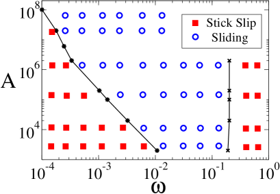
Figure 5: (color online) Phase diagram of model C. The points are located according to the values of the parameters $A$ and $\omega$ used in the simulations. The system transients from the stick–slip (squares) to the flowing (circles) phase on increasing the frequency or the amplitude, analogously to model A (see Fig. 1c). A second transition from the stick–slip to the flowing phase is observed at high frequencies.

However, this model also exhibits a second transition, in which friction is recovered. This transition is qualitatively analogous to that observed in Ref. capozza2009 . Indeed, when the oscillating plate’s frequency $\omega$ overcomes a critical value $\omega_{2}$, the system transients from the sliding to the stick–slip phase, as summarized in Fig. 5. This transition originates from the balance of the first two terms of Eq. (5), which regulates the dynamics of the block along the vertical direction. These two terms model elastic and dissipative forces along the direction $z^{\prime}$, and when they cancel out Eq. (5) admits the steady-state solution $k_{d}(x^{\prime}-V_{\textrm{d}}t)\sin(\alpha)=P_{l}$. The balance of these two terms

$$\gamma_{n}(\dot{z}^{\prime}-\dot{Z_{p}^{\prime}})\Theta(Z_{p}^{\prime}-z^{\prime})\geq k_{n}(Z_{p}^{\prime}-z^{\prime})\Theta(Z_{p}^{\prime}-z^{\prime}),$$ (11)

allows to estimate a transition frequency

$$\omega_{2}\geq\frac{k_{n}}{\gamma_{n}},$$ (12)

that is $A$ independent. This theoretical prediction is supported by the numerical results of Fig. 6, where we show that the recovery frequency $\omega_{2}$ weakly depends on $k_{n}$, when computed at a fixed $k_{n}/\gamma_{n}$ ratio. Contrary to the first transition, this second transition is not characterized by hysteresis, due to the important role of the dissipative mechanisms, which dominate over the inertial effects.

We wish to stress that the mechanism leading to the balance of the first two addends in the rhs of Eq. (1) does not lead to a stable solution for model A unless $mg=0$. This explains why the second transition is not observed in model A, and clarifies that this transition can only occur if an extra force is introduced in the rhs of Eq. (1) for the vertical component. The balance condition, Eq. (11), can be only satisfied in the presence of a modulated interface. Since there is no qualitative difference between model B and model C with respect to the motion along the vertical component $z^{\prime}$, this second transition is also observed in the vertical motion of model B. In both models, for fixed amplitude $A$, the block is embedded in the plate when $\omega<\omega_{1}$ and $\omega>\omega_{2}$, with $\omega_{2}$ given by Eq. (12). However, in model B this transition does not affect the motion along $x^{\prime}$ as this is only controlled by the stable solutions of Eq. (9). These solutions are not affected by $z^{\prime}-Z^{\prime}_{p}$, as previously discussed.

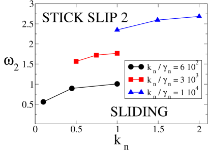
Figure 6:   (color online) Dependence of the friction recovery frequency $\omega_{2}$ on the elastic constant $k_{n}$, for different $k_{n}/\gamma_{n}$ ratios, as indicated.

III.4 Role of the driving velocity

Numerical simulations of confined Lennard–Jones particles gao have shown that the increase of the driving velocity $V_{d}$ leads the system to the sliding phase, also in the absence of an external perturbation. Here we show that this transition is reproduced by the models we have investigated.

In the model A, if the perturbation is turned off, there are two possible stationary solutions, depending on the non-linear behavior of the friction term $\mathcal{F}$. One is given by $x(t)=V_{S}\cdot t$, as described in Section II, and corresponds to a regime during which the friction term is $\mathcal{F}=V_{S}(t-t_{0})$. A second solution occurs when the friction term $k_{t}\mathcal{F}$ fluctuates so rapidly between its minimum (0) and its maximum ($\mu_{s}mg$) values that it can be replaced by its average value ($\mu_{s}mg/2$). This is the case when the typical time–scale for friction saturation (of order $\mu_{s}mg/(k_{t}V_{d})$ ) is much smaller than all the other time–scales of the system, which is certainly the case at very high $V_{d}$. The corresponding stationary solution is $x(t)=V_{d}t-x_{0}$, with $x_{0}=\gamma_{t}\cdot V_{d}/k_{d}-\mu_{s}mg/(2k_{d})$. The same arguments also apply to the models B and C. As an illustration, we report in Fig. 7 the phase diagram in the $(V_{d},\omega)$ plane of model C. The figure confirms the existence of a transition to the sliding phase for large driving velocity independently of $\omega$.

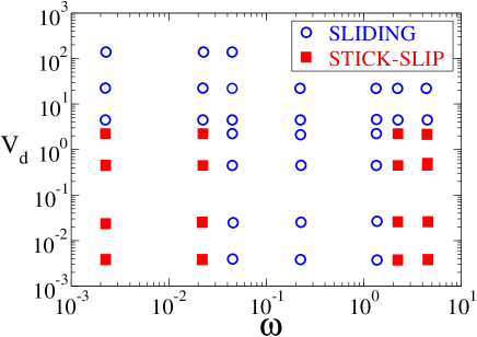
Figure 7: (color online) Phase diagram obtained for model C as a function of the driving velocity $V_{d}$. The symbols are located according to the values of the oscillation frequency $\omega$ and the velocity $V_{d}$ used in the simulations. The amplitude of the oscillation is set to the value $A=2\cdot 10^{4}$, while the other model parameters are the same used in the previous analysis of Section III C.

IV Conclusions

In order to understand the conditions under which mechanical vibrations suppress or enhance the frictional force between sliding objects, we have considered three variants of the usual spring–block model, in the presence of an history dependent frictional force. The models differ for the modulation of the surface over which the block slides, and for the direction of the confining force. In the model A and C, the equations of motion along the two directions are coupled, and on increasing the intensity of the perturbation we do observe a transition from the stick–slip to the sliding phase. Only in the presence of a modulated surface, and of a block confined by a force which is always normal to this surface, a further increase of the oscillation frequency leads to a second friction recovery transition, in which the system transients from the sliding to the stick–slip phase. This transition is analogous to that observed in Ref. capozza2009 in a Lennard–Jones system. Accordingly, our results clarify that the friction recovery transition is not a peculiarity of many particle systems, but rather a phenomenon linked to the modulation of the surface over which the block slides. In the model B mechanical vibrations do not affect the horizontal motion.

Our approach could be adapted to more complex models, suitable for the study of seismic phenomena, such as the many-blocks spring model. Further works include the investigation of different contact interactions, and of friction laws suggested by recent experimental results petri2010 .

- (1) M. Heuberger, C. Drummond and J. N. Israelachvili, J. Phys. Chem. B 102, 5038 (1998).
- (2) M. G. Rozman, M. Urbakh and J. Klafter, Phys. Rev. E 57, 7340 (1998).
- (3) J. P. Gao, W.D. Luedtke and U. Landman, J. Phys. Chem. B 102, 5033 (1998).
- (4) R. Capozza, A. Vanossi, A. Vezzani and S. Zapperi, Phys. Rev. Lett 103, 085502 (2009).
- (5) M. Urbakh, J. Klafter, D. Gourdon and J. Israelachvili, Nature 430, 29 (2004).
- (6) W. F. Brace and J. D. Byerlee, Science 153, 990 (1966).
- (7) J. Dieterich, J. Geophys. Res. 77, 3690 (1972).
- (8) A. Socoliuc, E. Gnecco, S. Maier, O.Pfeiffer, A. Baratoff, R. Bennewitz and E. Meyer, Science 313, 207 (2006).
- (9) E. Aharonov and D. Sparks, J. Geophys. Res. 109, B09306 (2004).
- (10) S. Nasuno, A. Kudrolli and J. P. Gollub, Phys. Rev. Lett. 79, 949 (1997).
- (11) J. C. Tsai, G. A. Voth and J. P. Gollub, Phys. Rev. Lett. 91, 064301 (2003).
- (12) P.A. Johnson and X. Jia, Nature 437, 871 (2005).
- (13) P. A. Johnson, He. Savage, M. Knuth, J. Gomberg and C. Marone, Nature 451, 57 (2008)
- (14) F. Dalton and D. Corcoran, Phys. Rev. E 63, 061312 (2001); F. Dalton and D. Corcoran, Phys. Rev. E 65, 031310 (2002).
- (15) C. Scholz, P. Molnar and T. Johnson, J. Geophys. Res. 77, 6392 6 (1972).
- (16) J. Dieterich, J. Geophys. Res. 84, 2161 (1979).
- (17) J. R. Rice, A. L. Ruina, J. Appl. Mech. 50, 343 (1983).
- (18) A. Helmstetter and B. E. Shaw, J. Geophys. Res. 114, B01308 (2009).
- (19) C. Marone, Nature 391, 69 1998.
- (20) S. Stacey, J. Gomberg and M. Cocco, J. Geophys. Res. 110, B05501 (2005).
- (21) M. Pica Ciamarra, E. Lippiello, C. Godano and L. de Arcangelis, Phys. Rev. Lett. 104, 238001 (2010).
- (22) M. Griffa, E. G. Daub, R. A. Guyer, P. A. Johnson, C. Marone and J. Carmeliet, Europhys. Lett. 96, 14001 (2011).
- (23) M. Pica Ciamarra, E. Lippiello, L. de Arcangelis and C. Godano, Europhys. Lett. 95, 54002 (2011).
- (24) G. L. Vasconcelos, Phys. Rev. Lett. 76, 4865 (1996).
- (25) C.H. Scholz, The mechanics of earthquakes and faulting, Cambridge University Press, 2002.
- (26) P. A. Cundall and O. D. L. Strack, Geotechnique 29, 47 (1979).
- (27) H. Risken, The Fokker-Plank Equation ( Springer-Verlag, Berlin, 1984).
- (28) M. Pica Ciamarra and A. Coniglio, Phys. Rev. Lett. 103, 235701 (2009).
- (29) T. Gyalog, M. Bammerlin, R. Luthi, E. Meyer and H. Thomas, Europhys. Lett. 31, 269 (1995).
- (30) F. Leoni, A. Baldassarri, F. Dalton, A. Petri, G. Pontuale and S. Zapperi, J. Non-Cryst. Solids 357, 749 (2011).