Teichmüller geodesics with $d$-dimensional limit sets

Abstract.

We construct an example of a Teichmüller geodesic ray whose limit set in Thurston boundary of Teichmüller space is an $d$-dimensional simplex.

1. Introduction

Thurston introduced a compactification of Teichmüller space of a surface $S$ using a boundary space $\mathcal{PMF}(S)$ consisting of projective classes of measured foliations [FLP79]. The boundary is homeomorphic to a sphere and the action of the mapping class group of the surface extends continuously to this boundary. In spite of the fact that Teichmüller metric is not negatively curved in any of the standard senses, using this compactification Thurston gave a classification of elements of mapping class groups in analogy with negatively curved spaces [FLP79].

In a hyperbolic space, every geodesic has a unique limit point. As a Teichmüller counterpart, Masur [Mas82] showed that the limit set of a Teichmüller geodesic ray with a uniquely ergodic vertical foliation is a single point. However, Kerckhoff [Ker80] showed that Thurston boundary is not the visual boundary of the Teichmüller metric.

In [Len08], Lenzhen gave the first example where the limit set of a Teichmüller geodesic ray is more than one point. The example is for a surface of genus two, and the limit set of the ray is an interval in one-dimensional simplex of measures for a non-minimal foliation in $\mathcal{PMF}(S)$. Since then, several other examples have been constructed. In [LLR13], it is shown that the same phenomenon can take place for a minimal foliation, with limit set being the entire one-dimensional simplex. In [CMW14] an example of minimal foliation is constructed where the limit set of the corresponding ray is a proper subset of a one-dimensional simplex of measures and in [BLMR16a] an example is constructed where the limit set is not simply connected and is homeomorphic to a circle. Similar phenomena is also possible for the geodesic in Teichmüller space equipped with the Weil-Petersson metric [BLMR16b, BLMR17]. However, so far in all the examples the limit set has been at most one-dimensional. Masur has asked if the limit set can ever have higher dimension. In this paper, we give a positive answer to the question of Masur.

Theorem 1.1.

For any $d\geq 2$, there exists a Teichmüller geodesic ray whose limit set in $\mathcal{PMF}(S)$ is $d$-dimensional.

The example is constructed as follows. Let $T^{i},\,i\in\mathbb{Z}_{d+1}=\{0,1,2,\ldots,d\}$, be a square torus rotated so that the vertical direction has a slope $\theta^{i}\in(0,1){\smallsetminus}\mathbb{Q}$ in $T^{i}$. Cut a vertical slit of size $s_{0}>0$ in $T_{i}$ and glue the left side of the slit of $T^{i}$ to the right side of $T^{i+1}$. We obtain a translation surface, that is, a Riemann surface $X_{0}$ of genus $d+1$ (see Figure 1), with a holomorphic quadratic differential $(X_{0},\phi_{0})$ with two zeros of order $2d$ where the restriction of the vertical foliation to $T^{i}$ has slope $\theta^{i}$. Let ${\bf r}$ be the Teichmüller geodesic ray based at $X_{0}$, and in the direction of $\phi_{0}$. For each $i=0,1,\ldots,d$, let $\nu^{i}$ be the ergodic measured foliation in $\mathcal{PMF}(S)$ supported on $T^{i}$, and defined by $\theta^{i}$.

Figure 1. Case $d=2$. The surface $X_{0}$ is glued out of three tori.

Theorem 1.1 is a consequence of the following statement.

Theorem 1.2.

There exist irrational numbers $\theta^{0},\theta^{1},\ldots,\theta^{d}$ such that the limit set of the corresponding ray ${\bf r}$ is the simplex of measures spanned by $\nu^{0},\nu^{1},\ldots,\nu^{d}$.

The irrational numbers $\theta^{i},\;i=0,\ldots,d,$ are defined via continued fraction expansions, where the coefficients of each continued fraction satisfies certain growth conditions (see $\S$3.1). The limit then is determined by estimating lengths of the curves corresponding to convergents of the continued fractions at different times along the ray r.

Acknowledgement

The second author was partially supported by NSF grant DMS-1065872. The third author was partially supported by NSERC Discovery grant RGPIN-435885. The authors would like to thank the referee for careful reading of the paper and many helpful comments.

2. Background

Notation

For a pair of sequences $\{x_{n}\}_{n\in\mathbb{N}}$ and $\{y_{n}\}_{n\in\mathbb{N}}$, we write $x_{n}\sim y_{n}$ if

$$\frac{x_{n}}{y_{n}}\to 1\quad\text{as}\quad n\to\infty.$$

Note that $\sim$ is an equivalence relation on sequences of numbers, in particular it is symmetric and transitive.

Let

$$P\mathbb{R}_{+}^{3}=\Big{\{}[r,s,u]\mathbin{\Big{|}}r,s,u>0,\quad(r,s,u)\equiv(\lambda r,\lambda s,\lambda u)\quad\forall\lambda>0\Big{\}}.$$

Similarly, for a pair of sequences $\{[a_{n}^{0},a_{n}^{1},a_{n}^{2}]\}_{n}$ and $\{[b_{n}^{0},b_{n}^{1},b_{n}^{2}]\}_{n}$ in $P\mathbb{R}^{3}$ we write

$$[a_{n}^{0},a_{n}^{1},a_{n}^{2}]\sim[b_{n}^{0},b_{n}^{1},b_{n}^{2}]\qquad\text{if, for $i\in\mathbb{Z}_{3}$},\qquad\frac{a_{n}^{i}}{a_{n}^{i+1}}\sim\frac{b_{n}^{i}}{b_{n}^{i+1}}.$$

The notation $\stackrel{{\scriptstyle{}_{\ast}}}{{\asymp}}$ means equal up to a multiplicative, $\stackrel{{\scriptstyle{}_{+}}}{{\asymp}}$ means equal up to an additive error and $\asymp$ means equal up to and additive and a multiplicative error with uniform constants. For example

$${\mathfrak{a}}\stackrel{{\scriptstyle{}_{\ast}}}{{\asymp}}{\mathfrak{b}}\quad\Longleftrightarrow\quad\frac{{\mathfrak{b}}}{K}\leq{\mathfrak{a}}\leq K\,{\mathfrak{b}},\qquad\text{for a uniform constant $K$}.$$

The notations $\stackrel{{\scriptstyle{}_{\ast}}}{{\succ}}$, $\stackrel{{\scriptstyle{}_{+}}}{{\succ}}$ and $\succ$ are similarly defined.

2.1. Continued fractions

Let $\theta=[a_{0};a_{1},a_{2},\ldots]$ be any positive number, and denote the $n-$th convergent of $\theta$ by $\frac{p_{n}}{q_{n}}$. That is

$$\frac{p_{n}}{q_{n}}=a_{0}+\cfrac{1}{a_{1}+\cfrac{1}{\dotsb+\cfrac{1}{a_{n}}}}.$$

We will need he following standard facts about continued fractions (see, for example, [Khi64]):

(2.1) $$q_{n}=a_{n}q_{n-1}+q_{n-2},$$

(2.2) $$\frac{1}{q_{n}+q_{n+1}}\leq|p_{n}-q_{n}\theta|\leq\frac{1}{q_{n+1}}.$$

2.2. Teichmüller theory

In this section we recall some background material mainly about Teichmüller space and Teichmüller geodesics and throughout set our notations. We assume that the reader is familiar with basic facts about Teichmüller space and the space of measured foliations. See for example [GL00] and [FLP79] for a thorough treatment of this material.

The Teichmüller space of a closed orientable surface $S$, denoted by $\mathcal{T}(S)$, is the space of equivalence classes of all marked Riemann surfaces homeomorphic to $S$ i.e. orientation preserving homeomorphisms $f:S\to X$, where $X$ is a Riemann surface; two marked surfaces $f_{1}:S\to X_{1}$ and $f_{2}:S\to X_{2}$ are equivalent if $f_{2}\circ f_{1}^{-1}:X_{1}\to X_{2}$ is isotopic to a biholomorphic map.

A measured foliation $\nu$ on $S$ is a foliation with pronged singularities and a transverse measure. The space of measured foliations of $S$ is equipped with the weak^∗ topology. The projective class of a measured foliation $\nu$ is the class of all measures which are positive multiples of $\nu$. We denote the space of projective measured foliations by $\mathcal{PMF}(S)$ which is equipped with the natural topology induced from the weak^∗ topology of the space of measured foliations.

A quadratic differential $(X,\phi)$ on a Riemann surface $X$ is a $(2,0)-$tensor with holomorphic coefficients; in a local coordinate $z$ it has the form $\phi(z)dz^{2}$ with $\phi(z)$ a holomorphic function. Around every point where $\phi(z)$ is not zero, there exist coordinates $\zeta=\xi+i\eta$, called natural coordinates, in which the quadratic differential can be represented as $d\zeta^{2}$ (see e.g. [GL00, §2]). There are two measured foliations naturally assigned to $\phi$. The trajectories $d\eta\equiv 0$ and $d\xi\equiv 0$ define the horizontal and vertical foliations of $\phi$, respectively. Integrating $|d\eta|$ and $|d\xi|$ along arcs determine horizontal and vertical measured foliations $\nu^{+}$ and $\nu^{-}$, respectively. Moreover, $(X,\phi)$ is defined uniquely by $X$ and its vertical measured foliation, by a theorem of Hubbard and Masur [HM79].

A Teichmüller geodesic can be described as follows. Given a quadratic differential $(X_{0},\phi_{0})$ on $X_{0}$, let $\zeta=\xi+i\eta$ be a natural coordinate for $(X_{0},\phi_{0})$. Then we can obtain a 1-parameter family $(X_{t},\phi_{t})$ of quadratic differentials defined locally by $d\zeta_{t}^{2}$ where $\zeta_{t}=e^{t}\xi+ie^{-t}\eta$. The map ${\bf g}:\mathbb{R}\to\mathcal{T}(S)$ which sends $t$ to $X_{t}$ is a Teichmüller geodesic. We will often write $(X_{t},\phi_{t})$ to refer to the geodesic. We will also denote by ${\bf r}$ the Teichmüller ray which is the image of $\mathbb{R}_{+}$.

Notions of length of a curve

By a curve we mean the free homotopy class of an essential simple closed curve. There are various notions of length associated to a curve $\alpha$ on a surface with a quadratic differential $(X,\phi)$.

We can equip $X$ with the hyperbolic metric in the conformal class of $X$ given by the uniformization. Then the hyperbolic length of $\alpha$, denoted by $\operatorname{Hyp}_{X}(\alpha)$, is the length of the geodesic representative of $\alpha$ on $X$.

The extremal length of $\alpha$ is defined by

(2.3) $$\operatorname{Ext}_{X}(\alpha)=\sup_{\rho\in[X]}\frac{\ell_{\rho}(\alpha)^{2}}{\operatorname{area}_{\rho}(X)}$$

where $\rho$ is any metric in the conformal class of $X$. The reciprocal of the extremal length is equal to the maximum modulus of any annulus with core curve $\alpha$ [GL00].

Maskit [Mas85] established the following relation between hyperbolic and extremal lengths:

(2.4) $$\frac{1}{\pi}\leq\frac{\operatorname{Ext}_{X}(\alpha)}{\operatorname{Hyp}_{X}(\alpha)}\leq\frac{1}{2}e^{\operatorname{Hyp}_{X}(\alpha)/2}.$$

When either $\operatorname{Hyp}_{X}(\alpha)$ or $\operatorname{Ext}_{X}(\alpha)$ is small, the above inequality implies that the two lengths are comparable,

(2.5) $$\operatorname{Hyp}_{X}(\alpha)\stackrel{{\scriptstyle{}_{\ast}}}{{\asymp}}\operatorname{Ext}_{X}(\alpha).$$

where the multiplicative constant depends only on an upper for the extremal or hyperbolic length of $\alpha^{i}$.

The quadratic differential $(X,\phi)$ defines a singular flat metric $|\phi(z)||dz|^{2}$ on $X$. The flat length of $\alpha$, denoted by $\ell_{\phi}(\alpha)$, is the length of a geodesic representative of $\alpha$ in this metric.

Finally, let $\alpha^{\prime}\sim\alpha$ be any curve in the homotopy class of $\alpha$. Recall then the notion of intersection number of a measured foliation $\nu$ and $\alpha$, defined by

$$\operatorname{i}(\alpha,\nu):=\inf_{\alpha^{\prime}\sim\alpha}\int_{\alpha^{\prime}}\nu.$$

This generalizes the usual notion of geometric intersection number of two curves.

Given a quadratic differential $\phi$ with corresponding horizontal and vertical measured foliations $\nu^{+}$ and $\nu^{-}$, the horizontal length of the curve $\alpha$ is $h_{\phi}(\alpha)=\operatorname{i}(\alpha,\nu^{-})$ and its vertical length is $v_{\phi}(\alpha)=\operatorname{i}(\alpha,\nu^{+})$.

Note that along a Teichmüller geodesic $(X_{t},\phi_{t})$ we have

$$h_{\phi_{t}}(\alpha)=e^{t}h_{\phi}(\alpha)\;\;\mbox{and}\;\;v_{\phi_{t}}(\alpha)=e^{-t}v_{\phi}(\alpha).$$

When the Teichmüller geodesic is fixed, to simplify our presentation we will often use the notations $\operatorname{Hyp}_{t}(\alpha)$, $\operatorname{Ext}_{t}(\alpha)$, $\ell_{t}(\alpha)$, $h_{t}(\alpha)$ and $v_{t}(\alpha)$ instead of writing $\operatorname{Hyp}_{X_{t}}(\alpha)$, $\operatorname{Ext}_{X_{t}}(\alpha)$, $\ell_{\phi_{t}}(\alpha)$, $h_{\phi_{t}}(\alpha)$ and $v_{\phi_{t}}(\alpha)$ respectively.

Balanced time

The balanced time of a curve $\alpha$ along a Teichmüller geodesic $(X_{t},\phi_{t})$ is the time when the horizontal and vertical lengths of $\alpha$ are equal:

$$h_{\phi_{t}}(\alpha)=v_{\phi_{t}}(\alpha).$$

If the geodesic representative of $\alpha$ in the flat metric $|\phi||dz|^{2}$ is neither vertical i.e. $h_{\phi}(\alpha)\neq 0$ nor horizontal i.e. $v_{\phi}(\alpha)\neq 0$, then there is a unique balanced time for the curve $\alpha$ along the geodesic which we denote by $t_{\alpha}$. The flat, extremal and hyperbolic lengths of $\alpha$ realize their minima in a uniformly bounded distance from the time $t_{\alpha}$. See [MM99, §2][Raf14] for more detail.

Twist parameter

Let $X$ be a point in $\mathcal{T}(S)$. For a curve $\alpha$ on $X$ let $Y_{\alpha}$ be the annular cover of $X$ associated to $\alpha$ i.e. the annular cover for which the curve $\alpha$ lifts to its core curve. Equip $Y_{\alpha}$ with the lift of the metric of $X$ and let $\overline{Y}_{\alpha}$ be the compactification of $Y_{\alpha}$ adding the ideal boundary. Let $\tau$ be an arc orthogonal to the core curve of $\overline{Y}_{\alpha}$ which connects the two boundaries of $\overline{Y}_{\alpha}$. Now the twist parameter of a curve $\gamma$ about the curve $\alpha$ is defined by

(2.6) $$\operatorname{twist}_{\alpha}(\gamma,X):=\operatorname{i}(\tilde{\gamma},\tau)$$

where $\tilde{\gamma}$ is any chosen lift of $\gamma$ that intersects the core of $\overline{Y}_{\alpha}$.

For a Teichmüller geodesic $(X_{t},\phi_{t})$ Rafi [Raf07a, Theorem 1.3] gives the following estimate for the twist parameter of a curve $\gamma$ about $\alpha$ at time $t$:

(2.7) $$\left|\operatorname{twist}_{\alpha}(\gamma,X_{t})\right| \leq \frac{c_{\gamma}}{\operatorname{Hyp}_{X_{t}}(\alpha)}\;\;\;\mbox{ if }t\leq t_{\alpha},$$

$$|\operatorname{twist}_{\alpha}(\gamma,X_{t})-\operatorname{i}_{\alpha}(\nu^{-},\nu^{+})| \leq \frac{c_{\gamma}}{\operatorname{Hyp}_{X_{t}}(\alpha)}\;\;\;\mbox{ if }t>t_{\alpha}.$$

Here, the number $\operatorname{i}_{\alpha}(\nu^{-},\nu^{+})$ is the maximum number that a leaf of the lift of $\nu^{-}$ and a leaf of the lift of $\nu^{+}$ to $Y_{\alpha}$ intersect. The number, up to an additive constant, is equal to the maximum of the number of times that a leaf of $\nu^{-}$ and a leaf of $\nu^{+}$ intersect inside of the maximal flat cylinder with core curve $\alpha$ (see below for more detail about the maximal flat cylinder). Finally, note that the constant $c_{\gamma}$ depends on $\gamma$.

Remark 2.1.

In fact, Rafi states the estimate for $\operatorname{twist}_{\alpha}(\nu^{+},X_{t})$, which using the fact that the intersection number $\operatorname{i}_{\alpha}(\cdot,\cdot)$ is quasi-additive and absorbing $\operatorname{i}_{\alpha}(\gamma,\nu^{+})$ in the $O$ notation constant gives us the above estimate.

In what follows we recall estimates for the extremal and hyperbolic lengths of a curve at a point in the Teichmüller space which we will use later in the paper.

An estimate for the extremal length of a curve

Using the flat structure of $(X,\phi)$, one can estimate the extremal length of a curve $\alpha$ on $X$. In general $\alpha$ does not have a unique geodesic representative with respect to the flat metric of $\phi$. However, the set of geodesic representatives foliate a (possibly degenerate) flat cylinder $F_{\alpha}$ in $(X,\phi)$. Let $f_{\alpha}$ be the distance between the boundaries of $F_{\alpha}$. Then $\operatorname{Mod}_{X}(F_{\alpha})=\frac{f_{\alpha}}{\ell_{\phi}(\alpha)}$ where $\operatorname{Mod}({\mathchoice{\mkern 1.0mu\mbox{\raise 2.2pt\hbox{$\centerdot$}}\mkern 1.0mu}{\mkern 1.0mu\mbox{\raise 2.2pt\hbox{$\centerdot$}}\mkern 1.0mu}{\mkern 1.5mu\centerdot\mkern 1.5mu}{\mkern 1.5mu\centerdot\mkern 1.5mu}})$ is the modulus of the annulus. For either boundary component of $F_{\alpha}$, we consider the largest one-sided regular neighborhood of $F_{\alpha}$ that is an embedded annulus. We denote these annuli by $E_{\alpha}$ and $G_{\alpha}$ respectively and refer to them as expanding annuli associated to $\alpha$. Denote the distance between boundaries of $E_{\alpha}$ and $G_{\alpha}$ (i.e., the radius of the associated regular neighborhood) by $e_{\alpha}$ and $g_{\alpha}$ respectively. When $e_{\alpha}>\ell_{\phi}(\alpha)$, we have

$$\operatorname{Mod}_{X}(E_{\alpha})\stackrel{{\scriptstyle{}_{\ast}}}{{\asymp}}\log\frac{e_{\alpha}}{\ell_{\phi}(\alpha)}.$$

The same holds for $g_{\alpha}$ and $G_{\alpha}$. We can then estimate the extremal length of $\alpha$ as follows (see [Min92, Raf14]):

(2.8) $$\frac{1}{\operatorname{Ext}_{X}(\alpha)}\stackrel{{\scriptstyle{}_{\ast}}}{{\asymp}}\operatorname{Mod}_{X}(E_{\alpha})+\operatorname{Mod}_{X}(F_{\alpha})+\operatorname{Mod}_{X}(G_{\alpha}).$$

An estimate for the hyperbolic length of a curve

Given $L>0$, let $P$ be a pants decomposition of $X$, i.e. a maximal collection of pairwise disjoint closed curves, with the property that the hyperbolic lengths of all curves in $P$ are at most $L$.

For a curve $\alpha$ on $X$ let the width of $\alpha$, $\operatorname{width}_{X}(\alpha)$, be the width of the collar around $\alpha$ from the Collar lemma [Bus92, §4.1]. We have the following estimate for the width

(2.9) $$\operatorname{width}_{X}(\alpha)=2\operatorname{arcsinh}{\frac{1}{\sinh(\frac{1}{2}\operatorname{Hyp}_{X}(\alpha))}}\stackrel{{\scriptstyle{}_{+}}}{{\asymp}}-2\log(\operatorname{Hyp}_{X}(\alpha)).$$

Now define the contribution to the length of a curve $\gamma$ from a curve $\alpha\in P$ by

(2.10) $$\operatorname{Hyp}_{X}(\gamma,\alpha)=\operatorname{i}(\gamma,\alpha)\big{(}\operatorname{width}_{X}(\alpha)+\operatorname{twist}_{X}(\gamma,\alpha)\operatorname{Hyp}_{X}(\alpha)\big{)}$$

where the additive constant depends only on the topological type of the surfaces. Then we have the following estimate for the hyperbolic length of a curve $\gamma$ in terms of the contributions from the curves in $P$,

(2.11) $$\big{|}\operatorname{Hyp}_{X}(\gamma)-\sum_{\alpha\in P}\operatorname{Hyp}_{X}(\gamma,\alpha)\big{|}=O\big{(}\sum_{\alpha\in P}\operatorname{i}(\gamma,\alpha)\big{)}.$$

where the constant of the $O$ notation depends only on $L$. See [CRS08, Lemma 3.7].

Growth of hyperbolic length along a Teichmüller geodesic

It follows from Wolpert’s estimate for the change of length [Wol79, Lemma 3.1] and the description of Teichmüller geodesics that the hyperbolic length of a curve varies at most exponentially along a Teichmüller geodesic. More precisely, given times $t,s\in\mathbb{R}$ with $t\geq s$ we have

(2.12) $$e^{-2|t-s|}\operatorname{Hyp}_{s}(\alpha)\leq\operatorname{Hyp}_{t}(\alpha)\leq e^{2|t-s|}\operatorname{Hyp}_{s}(\alpha)$$

The above inequality and the Equation (2.9) in particular show that the width of the collar of the curve $\alpha$ grows at most linearly along a Teichmüller geodesic.

Thurston boundary

The main purpose of this paper is the construction of Teichmüller geodesic rays with two-dimensional limit sets in the Thurston boundary. The Thurston boundary of the Teichmüller space $\mathcal{T}(S)$ is the space of projective measured foliations on $S$, $\mathcal{PMF}(S)$. A sequence of points $X_{n}\in\mathcal{T}(S)$ converges to the projective class of a measured foliation $[\nu]$ if and only if for any two curves $\gamma_{1},\gamma_{2}$ on $S$ we have

$$\lim_{n\to\infty}\frac{\operatorname{Hyp}_{X_{n}}(\gamma_{1})}{\operatorname{Hyp}_{X_{n}}(\gamma_{2})}=\frac{\operatorname{i}(\gamma_{1},\nu)}{\operatorname{i}(\gamma_{2},\nu)}.$$

The topology defined by this notion of convergence turns $\mathcal{T}(S)\cup\mathcal{PMF}(S)$ into a closed ball where $\mathcal{PMF}(S)$ is the boundary sphere. For more detail see [FLP79, exposé 8].

3. The Teichmüller geodesic ray and its limit set

In this section we prove our main result. First, in $\S$3.1, via continued fraction expansions, we define a measured foliation on $X_{0}$ and hence fix a Teichmüller ray based at $X_{0}$. Then, in $\S$3.2, we find the shortest pants decomposition at various times along the geodesic ray, to then be able to estimate hyperbolic length of curves using (2.11). In $\S$3.3 we use this information to determine the limit set of the Teichmüller ray and prove Theorem 1.2. To keep the exposition fairly simple, the proof given here is for $d=2$. For $d>2$ the notation is significantly heavier while the arguments are exactly the same.

3.1. Setup of continued fraction expansions

Let $\{[u^{0}_{k},u^{1}_{k},u^{2}_{k}]\}_{k\in\mathbb{N}}$ be a dense sequence in $P\mathbb{R}_{+}^{3}$ where $u^{0}_{k},u^{1}_{k},u^{2}_{k}\in\mathbb{N}$. Given this sequence, we will choose the numbers $\theta^{i}$ by describing their continued fraction expansion coefficients.

Let $\{a_{j}^{0}\}_{j\in\mathbb{N}},\{a_{j}^{1}\}_{j\in\mathbb{N}}$ and $\{a_{j}^{2}\}_{j\in\mathbb{N}}$ be three sequences of positive integers defined inductively as follows. Set $a_{1}^{0}=a_{1}^{1}=a_{1}^{2}=1$. Now, for $k\geq 1$ and $i\in\mathbb{Z}_{3}$, assume $a^{i}_{1},\ldots,a^{i}_{2k-1}$ are defined and whenever $n$ is such that $a^{i}_{1},\ldots,a^{i}_{n}$ are defined, let

$$\frac{p_{n}^{i}}{q_{n}^{i}}=\cfrac{1}{a_{1}^{i}+\cfrac{1}{\dotsb+\cfrac{1}{a_{n}^{i}}}}.$$

Choose $a_{2k}^{i},a_{2k+1}^{i}\in\mathbb{N}$ so that

1. $a_{2k}^{i}>k\cdot\max\big{\{}a_{2k-1}^{i},u^{0}_{k},u^{1}_{k},u^{2}_{k}\big{\}}$,

2. $[a_{2k}^{0},a_{2k}^{1},a_{2k}^{2}]=[u^{0}_{k},u^{1}_{k},u^{2}_{k}]$ as elements in $P\mathbb{R}_{+}^{3}$,

3. $a_{2k+1}^{i}>\exp(ka^{i}_{2k})$,

4. $a_{2k+1}^{0}q_{2k}^{0}=a_{2k+1}^{1}q_{2k}^{1}=a_{2k+1}^{2}q_{2k}^{2}$.

Define $\theta^{i}=[0;a_{1}^{i},a_{2}^{i},\ldots]\in(0,1)$. That is

$$\theta^{i}=\cfrac{1}{a_{1}^{i}+\cfrac{1}{a_{2}^{i}+\cfrac{1}{a_{3}^{i}+\dotsb}}}.$$

Lemma 3.1.

Let $\theta^{i},i\in\mathbb{Z}_{3}$ be as above. Then $\theta^{i}$ are irrational and, for every $k$ , we have

(3.1) $$q_{2k+1}^{0}=q_{2k+1}^{1}=q_{2k+1}^{2},$$

(3.2) $$[q_{2k}^{0},q_{2k}^{1},q_{2k}^{2}]\sim[u^{0}_{k},u^{1}_{k},u^{2}_{k}],$$

(3.3) $$\frac{\log{a_{2k+1}^{i}}}{\max\{a_{2k}^{i},u^{0}_{k},u^{1}_{k},u^{2}_{k}\}}\to\infty\;\text{as}\;k\to\infty,$$

(3.4) $$\log{a_{2k+1}^{0}}\sim\log{a_{2k+1}^{1}}\sim\log{a_{2k+1}^{2}},$$

(3.5) $$q_{n}^{i}\stackrel{{\scriptstyle{}_{\ast}}}{{\asymp}}\prod_{j=1}^{n}a_{j}^{i}.$$

Proof.

The irrationality of $\theta^{i}$ follows from the fact that the coefficients $a_{n}^{i}$ are non-zero.

We prove (3.1) by induction on $k$. By setup of the continued fraction expansion, we have $a^{0}_{1}=a^{1}_{1}=a^{2}_{1}$, and therefore $q^{0}_{1}=q^{1}_{1}=q^{2}_{1}$ by (2.1). Now assume that (3.1) holds for all $k^{\prime}$ less than or equal to some $k>1$. For each $i\in\mathbb{Z}_{3}$ we have that $q^{i}_{2k}=a^{i}_{2k}q^{i}_{2k-1}+q^{i}_{2k-2}$ by (2.1). Moreover, by (iv), for $i,j\in\mathbb{Z}_{3}$, we have $a^{i}_{2k+1}q^{i}_{2k}=a^{j}_{2k+1}q^{j}_{2k}$. These two equalities and assumption of the induction imply that (3.1) holds for $k$ as well.

To see (3.2), note that $a^{0}_{2k}=\frac{q^{0}_{2k}-q^{0}_{2k-2}}{q^{0}_{2k-1}}$ and $a^{1}_{2k}=\frac{q^{1}_{2k}-q^{1}_{2k-2}}{q^{1}_{2k-1}}$ by (2.1). Dividing these two numbers and taking into account that $q^{0}_{2k-1}=q^{1}_{2k-1}$ by (3.1) we get

$$\frac{a^{1}_{2k}}{a^{0}_{2k}}=\frac{q^{1}_{2k}-q^{1}_{2k-2}}{q^{0}_{2k}-q^{0}_{2k-2}}=\frac{q^{1}_{2k}}{q^{0}_{2k}}\frac{1-(q^{1}_{2k-2}/q^{1}_{2k})}{1-(q^{0}_{2k-2}/q^{0}_{2k})}.$$

The growth of the sequence $\{q^{i}_{k}\}_{k}$ from (i) and (iii) implies that $q^{1}_{2k-2}/q^{1}_{2k}$ and $q^{0}_{2k-2}/q^{0}_{2k}$ go to $0$ as $k\to\infty$. Therefore, $a^{0}_{2k}/a^{1}_{2k}\sim q^{0}_{2k}/q^{1}_{2k}$. But, by (ii), $a^{0}_{2k}/a^{1}_{2k}=u^{0}_{k}/u^{1}_{k}$. Hence

$$q^{0}_{2k}/q^{1}_{2k}\sim u^{0}_{k}/u^{1}_{k}.$$

Similarly, we can show that

$$q^{1}_{2k}/q^{2}_{2k}\sim u^{1}_{k}/u^{2}_{k}\;\;\text{and}\;\;q^{2}_{2k}/q^{0}_{2k}\sim u^{2}_{k}/u^{0}_{k}.$$

This finishes the proof of Equation (3.2).

To see (3.3), note that by (iii) we have

$$\frac{\log a^{i}_{2k+1}}{\max\{a^{i}_{2k},u^{0}_{k},u^{1}_{k},u^{2}_{k}\}}>\frac{ka^{i}_{2k}}{\max\{a^{i}_{2k},u^{0}_{k},u^{1}_{k},u^{2}_{k}\}}.$$

The term $\max\{a^{i}_{2k},u^{0}_{k},u^{1}_{k},u^{2}_{k}\}$ is either $a^{i}_{2k}$, or $\max\{u^{0}_{k},u^{1}_{k},u^{2}_{k}\}$. In the first situation, the right-hand side of the above inequality is equal to $k$. In the second situation, note that by (i), $\frac{a^{i}_{2k}}{\max\{u^{0}_{k},u^{1}_{k},u^{2}_{k}\}}>k$. Hence, the right-hand side of the above inequality is at least $k^{2}$. Thus in both cases the right-hand side goes to $\infty$ as $k\to\infty$, and therefore (3.3) holds.

Let us now prove (3.4). Without loss of generality suppose that $i=0$ and $j=1$. By (iv) we have

$$\log a_{2k+1}^{0}/\log a_{2k+1}^{1}=1+\frac{\log(q_{2k}^{1}/q_{2k}^{0})}{\log a_{2k+1}^{1}}.$$

Moreover, $\log(q_{2k}^{1}/q_{2k}^{0})\leq q_{2k}^{1}/q_{2k}^{0}$ and by (3.2) $q_{2k}^{1}/q_{2k}^{0}\sim u^{1}_{k}/u^{0}_{k}$. Then the right-hand side above goes to $1$, because by (3.3), $\frac{u^{1}_{k}}{u^{0}_{k}\log a_{2k+1}^{1}}\to 0$ as $k\to\infty$. This finishes the proof of (3.4).

We are left to prove Equation (3.5). It follows from Equation (2.1) that

$$q^{i}_{n}\geq\prod_{j=1}^{n}a_{j}^{i},$$

which is the lower bound in (3.5). For the upper bound, we write

$$\frac{q_{n}^{i}}{\prod_{j=1}^{n}a_{j}^{i}}=\frac{a_{n}^{i}q_{n-1}^{i}+q_{n-2}^{i}}{\prod_{j=1}^{n}a_{j}^{i}}\leq\frac{q_{n-1}^{i}}{\prod_{j=1}^{n-1}a_{j}^{i}}\left(1+\frac{1}{a_{n}^{i}}\right),$$

and so by an induction on $n$ we get

$$\frac{q_{n}^{i}}{\prod_{j=1}^{n}a_{j}^{i}}\leq\prod_{j=1}^{n}\left(1+\frac{1}{a_{j}^{i}}\right)<\prod_{n\geq 1}\left(1+\frac{1}{a_{n}^{i}}\right).$$

The infinite product on the right-hand side converges and is uniformly bounded for any sequence of coefficients $\{a_{n}^{i}\}_{n}$ that satisfies conditions (i) and (iii). ∎

For the rest of the paper let $(X_{0},\phi_{0})$ be the Riemann surface and quadratic differential obtained by gluing the three rotated square tori $T^{i}$ along vertical slits. The foliations $\nu^{i}$ on $T^{i}$ in the directions with slopes $\theta^{i}$, $i\in\mathbb{Z}_{3}$, glue together to make the vertical foliation $\nu$ of $\phi_{0}$.

3.2. Time and length estimates

Denote by $\alpha_{n}^{i}$ the simple curve on $T^{i}$ with slope $\frac{p_{n}^{i}}{q_{n}^{i}}$. Then we have the following.

Lemma 3.2.

For $i=0,1,2$ the curves $\alpha_{n}^{i}$ converge to $\nu^{i}$ in $\mathcal{PMF}(X_{0})$. More precisely, for any simple closed curve $\gamma$ on $X_{0}$,

(3.6) $$\frac{1}{q_{n}^{i}}\operatorname{i}(\gamma,\alpha_{n}^{i})\to\operatorname{i}(\gamma,\nu^{i})\sqrt{1+(\theta^{i})^{2}}.$$

Proof.

Suppose first that $\gamma$ is a curve on one of the tori, say $T^{i}$, and suppose that it has slope $\frac{p}{q}$. Then we have $\operatorname{i}(\gamma,\alpha_{n}^{i})=|pq_{n}^{i}-qp_{n}^{i}|$. On the other hand, the intersection number of $\gamma$ with $\nu^{i}$ is the absolute value of the dot product of the vector $(p,q)$ and the vector of unit length perpendicular to the foliation $\nu^{i}$, namely $\frac{1}{\sqrt{1+(\theta^{i})^{2}}}(\theta^{i},-1)$. Hence,

$$\operatorname{i}(\gamma,\nu^{i})=\frac{|p-q\theta^{i}|}{\sqrt{1+(\theta^{i})^{2}}}.$$

Since $\frac{p_{n}^{i}}{q_{n}^{i}}\to\theta^{i}$, we have

$$\frac{1}{q_{n}^{i}}\operatorname{i}(\gamma,\alpha_{n}^{i})=\left|p-q\frac{p_{n}^{i}}{q_{n}^{i}}\right|\to|p-q\theta^{i}|=\operatorname{i}(\gamma,\nu^{i})\sqrt{1+(\theta^{i})^{2}},$$

as $n\to\infty$, which is Equation (3.6) for $\gamma\subset T^{i}$. Now, since a measured foliation on $T^{i}$ is uniquely determined by its intersection number with all simple closed curves on $T^{i}$, it follows that

$$\frac{1}{q_{n}^{i}\sqrt{1+(\theta^{i})^{2}}}\alpha_{n}^{i}\to\nu^{i},\;\text{as $i\to\infty$}\qquad\text{in $\mathcal{MF}(T^{i})$}.$$

Furthermore, since $\mathcal{MF}(T^{i})$ embeds continuously into $\mathcal{MF}(X_{0})$, the sequence converges in $\mathcal{MF}(X_{0})$ as well. Thus, Equation (3.6) holds for all curves on $X_{0}$, which finishes proof of the lemma. ∎

From (3.2) in Lemma 3.1 and Lemma 3.2 we have

Corollary 3.3.

For any curve $\gamma$ on $X_{0}$, we have the following equivalence:

$$\sum_{i\in\mathbb{Z}_{3}}\operatorname{i}(\gamma,\alpha_{2k}^{i})\sim\frac{q_{2k}^{0}}{u^{0}_{k}}\left(\sum_{i\in\mathbb{Z}_{3}}u^{i}_{k}\sqrt{1+(\theta^{i})^{2}}\operatorname{i}(\gamma,\nu^{i})\right).$$

To estimate hyperbolic length of some fixed curve at a certain time along ${\bf r}$ using (2.11) we need information about the short curves at that time. The next lemma shows that the curves $\alpha_{n}^{i}$ become short along the ray ${\bf r}$ and gives estimates for the shortest lengths of the curves and the twist about them, also the times when the curves are shortest.

Lemma 3.4.

For $i\in\mathbb{Z}_{3}$ and $n\in\mathbb{N}$, the curve $\alpha_{n}^{i}$ is balanced at time

(3.7) $$t_{n}^{i}\stackrel{{\scriptstyle{}_{+}}}{{\asymp}}\frac{1}{2}\log{q_{n}^{i}q_{n+1}^{i}}\stackrel{{\scriptstyle{}_{+}}}{{\asymp}}\sum_{j=1}^{n}\log a_{j}^{i}+\frac{1}{2}\log a_{n+1}^{i}.$$

The flat length of $\alpha_{n}^{i}$ is minimal at $t_{n}^{i}$ and is given by

(3.8) $$\ell_{t_{n}^{i}}(\alpha_{n}^{i})\stackrel{{\scriptstyle{}_{\ast}}}{{\asymp}}\frac{1}{\sqrt{a_{n+1}^{i}}}.$$

Moreover, the extremal and hyperbolic lengths of $\alpha_{n}^{i}$ at $t_{n}^{i}$ are comparable and

(3.9) $$\operatorname{Ext}_{t^{i}_{n}}(\alpha^{i}_{n})\stackrel{{\scriptstyle{}_{\ast}}}{{\asymp}}\operatorname{Hyp}_{t^{i}_{n}}(\alpha_{n}^{i})\stackrel{{\scriptstyle{}_{\ast}}}{{\asymp}}\frac{1}{a_{n+1}^{i}}.$$

Finally, we have

(3.10) $$\operatorname{i}_{\alpha^{i}_{n}}(\nu^{-},\nu^{+})\stackrel{{\scriptstyle{}_{\ast}}}{{\asymp}}a^{i}_{n+1}$$

Proof.

The time when $\alpha_{n}^{i}$ is balanced can be computed explicitly. We have

(3.11) $$\ell_{t}(\alpha^{i}_{n})^{2}=h_{t}^{2}(\alpha^{i}_{n})+v_{t}^{2}(\alpha^{i}_{n}).$$

Since $h_{t}(\alpha^{i}_{n})=e^{t}\frac{1}{\sqrt{1+(\theta^{i})^{2}}}(p^{i}_{n}-\theta^{i}q^{i}_{n})$ and $v_{t}(\alpha^{i}_{n})=e^{-t}\frac{1}{\sqrt{1+(\theta^{i})^{2}}}(q^{i}_{n}+\theta^{i}p^{i}_{n})$, we have

(3.12) $$\ell_{t}(\alpha^{i}_{n})^{2}=\frac{1}{(1+(\theta^{i})^{2})}\Big{(}e^{-2t}(q^{i}_{n}+\theta^{i}p^{i}_{n})^{2}+e^{2t}(p^{i}_{n}-\theta^{i}q^{i}_{n})^{2}\Big{)}.$$

Now a straightforward calculation shows that $\ell_{t}(\alpha^{i}_{n})^{2}$ reaches its minimum at the time

(3.13) $$t_{n}^{i}=\frac{1}{2}\log\frac{p_{n}^{i}\theta^{i}+q_{n}^{i}}{|q_{n}^{i}\theta_{n}^{i}-p_{n}^{i}|}$$

(for more details see [Len08, Lemma 1]).

Remark 3.5.

In [Len08] Lenzhen uses the parametrization $\zeta_{t}=e^{t/2}\xi+ie^{-t/2}\eta$ for the Teichmüller geodesic, where $\zeta=\xi+i\eta$ is a natural coordinate at time $0$. But in this paper we use the parametrization $\zeta_{t}=e^{t}\xi+ie^{-t}\eta$ of the geodesic, which introduces the extra $\frac{1}{2}$ in the above formula.

By Equation (2.2) we have

(3.14) $$q^{i}_{n+1}(q^{i}_{n}\theta^{i}+p^{i}_{n})\leq\frac{p_{n}^{i}\theta^{i}+q_{n}^{i}}{|q_{n}^{i}\theta_{n}^{i}-p_{n}^{i}|}\leq(q^{i}_{n}+q^{i}_{n+1})(q^{i}_{n}\theta^{i}+p^{i}_{n}).$$

Now note that, $\lim_{n\to\infty}\frac{p^{i}_{n}}{q^{i}_{n}}=\theta^{i}$ and hence $q^{i}_{n}\stackrel{{\scriptstyle{}_{\ast}}}{{\asymp}}p^{i}_{n}$ for all sufficiently large $n$. Moreover, $\theta^{i}\in(0,1)$, in fact since $a^{i}_{1}=1$, we have that $\theta^{i}>\frac{1}{2}$, so the multiplicative constant in the coarse equality $q^{i}_{n}\stackrel{{\scriptstyle{}_{\ast}}}{{\asymp}}p^{i}_{n}$ is independent of $\theta^{i}$. Then by (3.14) and since $q^{i}_{n+1}\geq q^{i}_{n}$ we have

(3.15) $$\frac{p_{n}^{i}\theta^{i}+q_{n}^{i}}{|q_{n}^{i}\theta_{n}^{i}-p_{n}^{i}|}\stackrel{{\scriptstyle{}_{\ast}}}{{\asymp}}q^{i}_{n}q^{i}_{n+1}.$$

The equations (3.15) and (3.13) give us

$$t_{n}^{i}\stackrel{{\scriptstyle{}_{+}}}{{\asymp}}\frac{1}{2}\log q_{n}^{i}q_{n+1}^{i}.$$

The rest of Equation (3.7) now follows from Equation (3.5) of Lemma 3.1.

Moreover, since the times $t^{i}_{n}\to\infty$, it follows from [Len08, Lemma 3] and its proof, which essentially uses the fact that the area of the maximal flat cylinder $\operatorname{cyl}_{t}(\alpha_{n}^{i})$ with core curve $\alpha_{n}^{i}$ tends to 1, that

(3.16) $$\ell_{t^{i}_{n}}(\alpha^{i}_{n})^{2}\sim\operatorname{Ext}_{t^{i}_{n}}(\alpha^{i}_{n})\sim\frac{1}{\operatorname{Mod}(\operatorname{cyl}_{t^{i}_{n}}(\alpha^{i}_{n}))}.$$

Furthermore, the fact that by definition the sequence $a^{i}_{n}$ goes to infinity and (2.2) imply that

$$\ell_{t^{i}_{n}}(\alpha^{i}_{n})^{2}\sim\frac{2q^{i}_{n}}{q^{i}_{n+1}}\sim\frac{2}{a^{i}_{n+1}},$$

(for more detail see the proof of [Len08, Corollary 1]). This gives us (3.8).

Then Equation (3.9) follows from the comparison of extremal and hyperbolic lengths (2.5).

Finally, by [CRS08, Proposition 5.8], we have

$$\operatorname{i}_{\alpha^{i}_{n}}(\nu^{-},\nu^{+})\stackrel{{\scriptstyle{}_{\ast}}}{{\asymp}}\operatorname{Mod}(\operatorname{cyl}_{t^{i}_{n}}(\alpha^{i}_{n}))$$

as long as $\operatorname{Ext}_{t^{i}_{n}}(\alpha^{i}_{n})$, up to a bounded multiplicative constant, is $\frac{1}{\operatorname{Mod}(\operatorname{cyl}_{t^{i}_{n}}(\alpha^{i}_{n}))}$, which is the case by Equation (3.16). Equation (3.10) now follows from Equation (3.9). This finishes the proof of the lemma. ∎

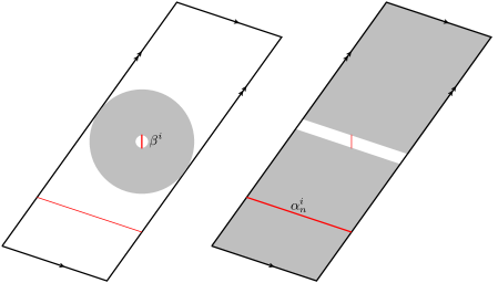
Figure 2. Annuli in $T^{i}$ about $\beta^{i}$ and $\alpha_{n}^{i}$. Expanding annulus with core curve $\beta^{i}$, on the left, and flat annulus about $\alpha_{n}^{i}$, on the right, at the time when $\alpha_{n}^{i}$ is balanced.

There are three other curves, namely $\beta^{i}=\partial T^{i}$, that become very short along ${\bf r}$. In fact, the length of $\beta^{i}$ goes to $0$. We have the following estimate for the length of $\beta^{i}$:

Lemma 3.6.

For $i\in\mathbb{Z}_{3}$ we have

(3.17) $$\operatorname{Hyp}_{t_{n}^{i}}(\beta^{i})\stackrel{{\scriptstyle{}_{\ast}}}{{\asymp}}\frac{1}{\log{q_{n}^{i}}}$$

Proof.

Starting with the proof, note that since the curve $\beta^{i}$ is homotopic to the union of two critical trajectories of the quadratic differential $\phi$ connecting two critical points of $\phi$ (see Figure 1), the flat length of $\beta^{i}$ is

$$\ell_{t_{n}^{i}}(\beta^{i})=2s_{0}e^{-t_{n}^{i}},$$

where $s_{0}$ is the size (flat length) of the slit we cut on the tori $T^{i}$, $i\in\mathbb{Z}_{3}$, to produce the initial genus three flat surface. Moreover, the shortest curve on $T^{i}$ at $t_{n}^{i}$ is $\alpha_{n}^{i}$, which is balanced and whose flat length satisfies

$$\ell_{t_{n}^{i}}(\alpha_{n}^{i})\stackrel{{\scriptstyle{}_{\ast}}}{{\asymp}}\frac{1}{\sqrt{a_{n+1}^{i}}}$$

by Lemma 3.4. Now by the two estimates above

$$\log\frac{\ell_{t^{i}_{n}}(\alpha^{i}_{n})}{\ell_{t^{i}_{n}}(\beta^{i})} \stackrel{{\scriptstyle{}_{+}}}{{\asymp}} t^{i}_{n}-\frac{1}{2}\log a^{i}_{n+1}$$

$$\stackrel{{\scriptstyle{}_{+}}}{{\asymp}} \sum_{j=1}^{n}\log a^{i}_{j}\stackrel{{\scriptstyle{}_{+}}}{{\asymp}}\log q^{i}_{n}$$

where the second equality holds by (3.7) in Lemma 3.4 and the third equality by (3.5) in Lemma 3.1.

Further, note that there is no flat annulus around $\beta^{i}$, and the distance between boundaries of the largest embedded neighborhood of $\beta^{i}$ inside $T^{i}$ is

$$\frac{\ell_{t^{i}_{n}}(\alpha^{i}_{n})-\ell_{t^{i}_{n}}(\beta^{i})}{2}$$

(see the right-hand side of Figure 2). Hence by Equation (2.8) we have

(3.19) $$\frac{1}{\operatorname{Ext}_{t_{n}^{i}}(\beta^{i})}\stackrel{{\scriptstyle{}_{\ast}}}{{\asymp}}\log\left(\frac{\ell_{t^{i}_{n}}(\alpha^{i}_{n})-\ell_{t^{i}_{n}}(\beta^{i})}{2\ell_{t^{i}_{n}}(\beta^{i})}\right)=\log\left(\frac{\ell_{t^{i}_{n}}(\alpha^{i}_{n})}{\ell_{t^{i}_{n}}(\beta^{i})}-1\right)-\log 2.$$

Also since $q^{i}_{n}\to\infty$ as $n\to\infty$, by (3.2) we have $\frac{\ell_{t^{i}_{n}}(\alpha^{i}_{n})}{\ell_{t^{i}_{n}}(\beta^{i})}\to\infty$ as $n\to\infty$. Thus from (3.19) we may deduce that

$$\frac{1}{\operatorname{Ext}_{t_{n}^{i}}(\beta^{i})}\stackrel{{\scriptstyle{}_{\ast}}}{{\asymp}}\log\frac{\ell_{t^{i}_{n}}(\alpha^{i}_{n})}{\ell_{t^{i}_{n}}(\beta^{i})}.$$

Then appealing again to (3.2) we have that the extremal length of $\beta^{i}$ at $t_{n}^{i}$ satisfies

$$\operatorname{Ext}_{t_{n}^{i}}(\beta^{i})\stackrel{{\scriptstyle{}_{\ast}}}{{\asymp}}\frac{1}{\log{q_{n}^{i}}}.$$

The lemma now follows from Maskit’s comparison of hyperbolic and extremal lengths (2.5). ∎

The following lemma follows from the proof of [Raf07a, Theorem 1.2]).

Lemma 3.7.

For any $i\in\mathbb{Z}_{3}$ and any $t>s$, the hyperbolic length of $\beta^{i}$ satisfies

(3.20) $$\frac{1}{\operatorname{Hyp}_{s}(\beta^{i})}\succ\frac{1}{\operatorname{Hyp}_{t}(\beta^{i})}.$$

This and Lemma 3.6 imply

Corollary 3.8.

For $i\in\mathbb{Z}_{3}$ and for $t\in[t_{n}^{i},t_{n+1}^{i}]$ we have

(3.21) $$\operatorname{Hyp}_{t_{n+1}^{i}}(\beta^{i})\stackrel{{\scriptstyle{}_{\ast}}}{{\prec}}\operatorname{Hyp}_{t}(\beta^{i})\stackrel{{\scriptstyle{}_{\ast}}}{{\prec}}\operatorname{Hyp}_{t_{n}^{i}}(\beta^{i}).$$

In particular,

(3.22) $$\underset{t\to\infty}{\lim}\operatorname{Hyp}_{t}(\beta^{i})=0.$$

Proof.

Let $t\geq t_{n}^{i}$. By Lemma 3.7 there is $K\geq 1$ independent of $t$ and $t_{n}^{i}$ such that

$$\frac{1}{\operatorname{Hyp}_{t}(\beta^{i})}\geq\frac{1}{K\operatorname{Hyp}_{t_{n}^{i}}(\beta^{i})}-K.$$

From Lemma 3.6 and the fact that $q^{i}_{n}\to\infty$ we see that the expression on the right is positive for $n$ big enough, and hence

$$\operatorname{Hyp}_{t}(\beta^{i})\stackrel{{\scriptstyle{}_{\ast}}}{{\prec}}\operatorname{Hyp}_{t_{n}^{i}}(\beta^{i}).$$

The other inequality can be shown in a similar way. Now, since along $\{t_{n}^{i}\}_{n}$ the hyperbolic length of $\beta^{i}$ goes to 0, we are done. ∎

3.3. The limit set

To find the limit set of the geodesic ray ${\bf r}$, we examine the geometry of Riemann surface $X_{t_{n}}$ for a carefully chosen sequence of times $\{t_{n}\}_{n}$. The curves $\beta^{i}$ are always short and the curves $\alpha^{i}_{2n}$ get short roughly at the same time $t_{n}$. The hyperbolic length of any given curve $\gamma$ can be computed as the sum of the contributions to the length of $\gamma$ coming from crossing the short curves in $X_{t_{n}}$. We will see that the contribution from $\alpha^{i}_{2n}$ dominates the contribution from $\beta^{i}$. But the curves $\alpha^{i}_{2n}$ are chosen so that the length contributions coming from these curves, thought of as a projective triple, form a dense subset of $P\mathbb{R}^{3}$. This will let us conclude that the limit set of the ray ${\bf r}$ contains the whole simplex of projective measures. The fact that the limit is contained in the simplex follows from a similar argument showing that asymptotically along the ray the contribution of $\beta^{i}$ to the length of $\gamma$ is negligible.

Proof of Theorem 1.2.

We first show that the limit set of ${\bf r}$ contains the simplex spanned by projective classes of the measures $\nu^{0},\nu^{1}$ and $\nu^{2}$. For this purpose we show that there exists a sequence of times $t_{n}\to\infty$ such that, given any two curves $\gamma_{1}$ and $\gamma_{2}$ not equal to $\beta^{i},i\in\mathbb{Z}_{3}$, we have

(3.23) $$\frac{\operatorname{Hyp}_{t_{n}}(\gamma_{1})}{\operatorname{Hyp}_{t_{n}}(\gamma_{2})}\sim\frac{\sum_{i\in\mathbb{Z}_{3}}w^{i}_{n}\operatorname{i}(\gamma_{1},\nu^{i})}{\sum_{i\in\mathbb{Z}_{3}}w^{i}_{n}\operatorname{i}(\gamma_{2},\nu^{i})}$$

where $w^{i}_{n}=u^{i}_{n}\sqrt{1+(\theta^{i})^{2}}$, $i\in\mathbb{Z}_{3}$. But the set $\{[u^{0}_{n},u^{1}_{n},u^{2}_{n}]\}_{n\in\mathbb{N}}$ is dense in $P\mathbb{R}_{+}^{3}$ and the map

$$[a,b,c]\to\Big{[}a\sqrt{1+(\theta^{0})^{2}},b\sqrt{1+(\theta^{1})^{2}},c\sqrt{1+(\theta^{2})^{2}}\Big{]}$$

is a homeomorphism of $P\mathbb{R}_{+}^{3}$, thus $\{[w^{0}_{n},w^{1}_{n},w^{2}_{n}]\}_{n\in\mathbb{N}}$ is also dense in $P\mathbb{R}_{+}^{3}$. Now by the definition given in $\S$2.2 for convergence in the Thurston compactification, the fact that $\{[w^{0}_{n},w^{1}_{n},w^{2}_{n}]\}_{n\in\mathbb{N}}$ is dense in $P\mathbb{R}_{+}^{3}$ and that the limit set is closed imply that every point in the simplex is in the limit set of ${\bf r}$.

We proceed by showing (3.23). As before denote the balanced time of $\alpha^{i}_{n}$ along ${\bf r}$ by $t^{i}_{n}$. Let $t_{n}$ be any number in the interval $\Big{[}\underset{i=0,1,2}{\min}\,t_{2n}^{i},\underset{i=0,1,2}{\max}\,t_{2n}^{i}\Big{]}$.

The point of choosing such $t_{n}$ is that (see Figure 3) as we will see below, all three curves $\alpha_{2n}^{i},i\in\mathbb{Z}_{3}$ are very short on $X_{t_{n}}$. Moreover, their collars are asymptotically of the same width.

For any $i,j\in\mathbb{Z}_{3}$ by Lemma 3.4 and Lemma 3.1(3.1) we have

$$|t_{2n}^{i}-t_{n}|\leq\max_{i,j=0,1,2}|t_{2n}^{i}-t_{2n}^{j}| \stackrel{{\scriptstyle{}_{+}}}{{\asymp}} \frac{1}{2}\max_{i,j=0,1,2}|\log q_{2n}^{i}-\log q_{2n}^{j}|$$

$$= \frac{1}{2}\max_{i,j=0,1,2}|\log(q_{2n}^{i}/q_{2n}^{j})|.$$

Moreover, by Lemma 3.1(3.2), for any $i,j\in\mathbb{Z}_{3}$, we have $q^{i}_{2n}/q^{j}_{2n}\sim u^{i}_{n}/u^{j}_{n}$, and hence $|\log q^{i}_{2n}/q^{j}_{2n}-\log u^{i}_{n}/u^{j}_{n}|\to 0$ as $n\to\infty$. Therefore,

$$\Big{|}\max_{i,j=0,1,2}|\log(q_{2n}^{i}/q_{2n}^{j})|-\max_{i,j=0,1,2}|\log(u_{n}^{i}/u_{n}^{j})|\Big{|}\to 0,$$

as $n\to\infty$. Thus for $n$ large enough

$$2|t_{2n}^{i}-t_{n}|\stackrel{{\scriptstyle{}_{+}}}{{\prec}}\max_{j=0,1,2}\log(u_{n}^{j}).$$

Then by Lemma 3.1 (3.3) we have that

(3.24) $$e^{2|t_{n}-t_{2n}^{i}|}=o(\log a_{2n+1}^{i}).$$

Now the estimate (3.9) in Lemma 3.4 and the estimate (3.24) together with the growth bound (2.12) give us

$$\operatorname{Hyp}_{t_{n}}(\alpha^{i}_{2n})\leq\operatorname{Hyp}_{t^{i}_{2n}}(\alpha^{i}_{2n})e^{2|t_{n}-t^{i}_{2n}|}\stackrel{{\scriptstyle{}_{\ast}}}{{\prec}}\frac{o(\log a_{2n+1}^{i})}{a^{i}_{2n+1}},$$

also $a^{i}_{2n+1}\to\infty$ as $n\to\infty$, so the last fraction in the above inequality goes to $0$. Therefore, for all $n$ sufficiently large, the hyperbolic lengths of the curves $\alpha_{2n}^{i}$, $i\in\mathbb{Z}_{3}$, at $X_{t_{n}}$ are uniformly bounded and in fact very small. Also from (3.22) of Corollary 3.8 we know that the hyperbolic lengths of $\beta_{i},\,i\in\mathbb{Z}_{3}$, are also uniformly bounded along $\bf r$.

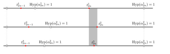
Figure 3. The interval when $\alpha_{k}^{i}$ is short. For $k=2n$, the curves $\alpha_{k}^{i},\;i\in\mathbb{Z}_{3}$, start getting short at different times, but they grow back to length 1 roughly at the same time. We choose $t_{n}$ in the shaded interval to guarantee that all three curves are short and have collar neighborhoods of approximately the same width.

Thus the collection of curves $\{\alpha^{i}_{2n},\beta^{i}\}_{i\in\mathbb{Z}_{3}}$ forms a bounded length pants decomposition at time $t_{n}$. Then by (2.11) we have the following estimate for the hyperbolic length of an arbitrary curve $\gamma$ on $X_{t_{n}}$:

(3.25) $$\operatorname{Hyp}_{t_{n}}(\gamma)= \sum_{i=0}^{2}\operatorname{Hyp}_{t_{n}}(\gamma,\alpha^{i}_{2n})+\sum_{i=0}^{2}\operatorname{Hyp}_{t_{n}}(\gamma,\beta^{i})$$

$$+ O\left(\sum_{i=0}^{2}\operatorname{i}(\gamma,\alpha_{2n}^{i})+\operatorname{i}(\gamma,\beta^{i})\right),$$

where the constant of $O$ notation depends only on an upper bound for the hyperbolic length of the curves $\alpha^{i}_{2n},\beta^{i},\;i\in\mathbb{Z}_{3},$ at time $t_{2n}$. We will now analyze the ingredients of this equation.

Intersection numbers

Note that, for any fixed curve $\gamma$, the intersection number with $\beta^{i}$ is clearly a constant, i.e.

(3.26) $$\operatorname{i}(\beta^{i},\gamma)\stackrel{{\scriptstyle{}_{+}}}{{\asymp}}0.$$

By Lemma 3.2 we have $\frac{\alpha^{i}_{2n}}{q^{i}_{2n}\sqrt{1+(\theta^{i})^{2}}}\to\nu^{i}$, hence, by continuity of intersection numbers [Bon88], we have

$$\operatorname{i}\left(\gamma,\frac{\alpha^{i}_{2n}}{q^{i}_{2n}\sqrt{1+(\theta^{i})^{2}}}\right)\to\operatorname{i}(\gamma,\nu^{i}).$$

Thus

(3.27) $$\operatorname{i}(\gamma,\alpha^{i}_{2n})\stackrel{{\scriptstyle{}_{\ast}}}{{\asymp}}q^{i}_{2n}.$$

Contribution to the length of $\gamma$ from the curves $\alpha^{i}_{2n}$ at $t_{n}$

First, the hyperbolic length of $\alpha_{2n}^{i}$ by inequality (2.12) and the inequality (3.9) from Lemma 3.4 satisfies

$$\frac{1}{a_{2n+1}^{i}}e^{-2|t_{n}-t_{2n}^{i}|}\stackrel{{\scriptstyle{}_{\ast}}}{{\prec}}\operatorname{Hyp}_{t_{n}}(\alpha_{2n}^{i})\stackrel{{\scriptstyle{}_{\ast}}}{{\prec}}\frac{1}{a_{2n+1}^{i}}e^{2|t_{n}-t_{2n}^{i}|},$$

which using the fact that by Equation (2.9), $\operatorname{width}_{t^{i}_{2n}}(\alpha^{i}_{2n})\stackrel{{\scriptstyle{}_{+}}}{{\asymp}}-2\log\left(\operatorname{Hyp}_{t^{i}_{2n}}(\alpha^{i}_{2n})\right)$ implies the following estimate

$$\operatorname{width}_{t_{n}}(\alpha_{2n}^{i})\stackrel{{\scriptstyle{}_{+}}}{{\asymp}}2\log{a_{2n+1}^{i}}\pm O(2|t_{n}-t_{2n}^{i}|).$$

Then, by Equation (3.24), Lemma 3.1 (3.3) and the fact that $a^{i}_{2n+1}\to\infty$ we deduce that the widths of the collars of the curves $\alpha_{2n}^{i}$, $i\in\mathbb{Z}_{3}$, are equivalent, and that

(3.28) $$\operatorname{width}_{t_{n}}(\alpha_{2n}^{i})\sim 2\log{a_{2n+1}^{i}}.$$

By (3.10) in Lemma 3.4 and the formula (2.7) for twist parameters along Teichmüller geodesics we have

$$\operatorname{twist}_{\alpha_{2n}^{i}}(\gamma,X_{t_{n}})\stackrel{{\scriptstyle{}_{\ast}}}{{\prec}}a_{2n+1}^{i},$$

using Equation (3.24) then we have

(3.29) $$\operatorname{Hyp}_{t_{n}}(\alpha_{2n}^{i})\operatorname{twist}_{\alpha_{2n}^{i}}(\gamma,X_{t_{n}})\stackrel{{\scriptstyle{}_{\ast}}}{{\prec}}e^{2|t_{n}-t_{2n}^{i}|}=o(\log a_{2n+1}^{i}).$$

Now by (3.28) and (3.29) the contribution of $\alpha_{2n}^{i}$ to the length of $\gamma$ satisfies

(3.30) $$\operatorname{Hyp}_{t_{n}}(\gamma,\alpha^{i}_{2n})\sim 2\operatorname{i}(\gamma,\alpha^{i}_{2n})\log{a_{2n+1}^{i}}.$$

Contribution to the length of $\gamma$ from the curves $\beta^{i}$ at $t_{n}$

From (3.24) we have $2|t_{n}-t^{i}_{2n}|=o(\log\log a^{i}_{2n+1})$. Moreover by Equation (3.7) in Lemma 3.4 we have $t^{i}_{2n+1}-t^{i}_{2n}\stackrel{{\scriptstyle{}_{+}}}{{\succ}}\log a^{i}_{2n+1}$. Therefore, we have $t_{n}<t_{2n+1}^{i}$ for all $n$ sufficiently large.

Now applying (3.21) and Lemma 3.6 we get

(3.31) $$\operatorname{Hyp}_{t_{n}}(\beta^{i})\stackrel{{\scriptstyle{}_{\ast}}}{{\succ}}\frac{1}{\log{q_{2n+1}^{i}}},$$

which by the fact that $\operatorname{width}_{t_{n}}(\beta^{i})\stackrel{{\scriptstyle{}_{+}}}{{\asymp}}-2\log(\operatorname{Hyp}_{t_{n}}(\beta^{i}))$ implies that

(3.32) $$\operatorname{width}_{t_{n}}(\beta^{i})\stackrel{{\scriptstyle{}_{+}}}{{\prec}}2\log\log{q_{2n+1}^{i}}.$$

Moreover, by (3.5) in Lemma 3.1 we have $\log\log{q_{2n+1}^{i}}\stackrel{{\scriptstyle{}_{+}}}{{\asymp}}\log(\sum_{j=1}^{2n+1}\log a^{i}_{j})$. Now conditions (i) and (iii) from the setup of the continued fractions in $\S$3.1 imply that for each $i\in\mathbb{Z}_{3}$ the sequence $\{a^{i}_{j}\}_{j}$ is increasing, in fact it is increasing at least exponentially fast. Hence

$$\log(\sum_{j=1}^{2n+1}\log a^{i}_{j}) \leq \log((2n+1)\log{a^{i}_{2n}})$$

$$= \log{(2n+1)}+\log\log a^{i}_{2n+1}\stackrel{{\scriptstyle{}_{\ast}}}{{\asymp}}\log\log a^{i}_{2n+1}.$$

We then have that

(3.33) $$\operatorname{width}_{t_{n}}(\beta^{i})\stackrel{{\scriptstyle{}_{\ast}}}{{\prec}}\log\log{a_{2n+1}^{i}}.$$

Moreover, since $\beta^{i}$ is a union of critical trajectories, it does not have a flat cylinder neighborhood. Therefore, $\operatorname{i}_{\beta^{i}}(\nu^{-},\nu^{+})\stackrel{{\scriptstyle{}_{+}}}{{\asymp}}0$. Then, by (2.7), we have

(3.34) $$\operatorname{Hyp}_{t_{n}}(\beta^{i})\operatorname{twist}_{\beta^{i}}(\gamma,X_{t_{n}})\leq K_{\gamma},$$

where $K_{\gamma}\geq 0$ depends only on $\gamma$.

Hence by equations (3.26), (3.33), (3.34) and Corollary 3.8, the contribution to the length of $\gamma$ from the curve $\beta^{i}$ for $i\in\mathbb{Z}_{3}$ at time $t_{n}$ satisfies

(3.35) $$\operatorname{Hyp}_{t_{n}}(\gamma,\beta^{i}) = \operatorname{i}(\gamma,\beta^{i})\left(\operatorname{width}_{t_{n}}(\beta^{i})+\operatorname{Hyp}_{t_{n}}(\beta^{i})\operatorname{twist}_{\beta^{i}}(\gamma,X_{t_{n}})\right)$$

$$\stackrel{{\scriptstyle{}_{\ast}}}{{\prec}} \operatorname{i}(\gamma,\beta^{i})(\log\log a^{i}_{2n+1}+K_{\gamma})=o(\log a^{i}_{2n+1}).$$

We are now ready to establish Equation (3.23). First, we use Equation (3.25) and equations (3.26), (3.30) and (3.35) for the curves $\gamma_{1}$ and $\gamma_{2}$ to get

(3.36) $$\frac{\operatorname{Hyp}_{t_{n}}(\gamma_{1})}{\operatorname{Hyp}_{t_{n}}(\gamma_{2})}\sim\frac{\sum_{i=0}^{2}\operatorname{i}(\gamma_{1},\alpha_{2n}^{i})\log{a_{2n+1}^{i}}}{\sum_{i=0}^{2}\operatorname{i}(\gamma_{2},\alpha_{2n}^{i})\log{a_{2n+1}^{i}}}\sim\frac{\sum_{i=0}^{2}\operatorname{i}(\gamma_{1},\alpha_{2n}^{i})}{\sum_{i=0}^{2}\operatorname{i}(\gamma_{2},\alpha_{2n}^{i})},$$

where the second comparison holds by Equation (3.4) in Lemma 3.1. Then Corollary 3.3 applied to Equation (3.36) gives us the desired Equation (3.23).

As we saw above the limit set of ${\bf r}$ contains the simplex of projective measures spanned by $[\nu^{i}]$, $i\in\mathbb{Z}_{3}$. To complete the proof of the theorem it remains to show that the limit set of ${\bf r}$ is also contained in the simplex. First, note that any limit point of ${\bf r}$ has zero intersection number with the vertical measured foliation $\nu$ of $\phi_{0}$ which is the disjoint union of foliations $\nu^{i}$ and curves $\beta^{i},$ $\;i\in\mathbb{Z}_{3}$. Hence all we need to show is that every point in the limit set has zero weight on $\beta^{i},\,i\in\mathbb{Z}_{3}$.

For this purpose suppose that for a sequence of times $\{t_{k}\}_{k}$ the sequence $\{{\bf r}(t_{k})\}_{k}$ converges to the projective class of some measured foliation $\mu$ in $\mathcal{PMF}(S)$. Then as is shown in [FLP79, expośe 8] there is a sequence $\{s_{k}\}_{k}$ with $s_{k}\to 0$, so that for any simple closed curve $\gamma$ we have

(3.37) $$\lim_{k\to\infty}s_{k}\operatorname{Hyp}_{t_{k}}(\gamma)=\operatorname{i}(\gamma,\mu).$$

To show that $\mu$ has zero weight on $\beta^{i}$ for all $i\in\mathbb{Z}_{3}$, we argue as follows.

Given $i\in\mathbb{Z}_{3}$ let $\gamma$ be any simple closed curve that intersects $\beta_{i}$ twice and does not intersect any $\beta_{j}$ with $j\neq i$. Let $\gamma^{\prime}\subset T_{i}$ be a simple closed curve obtained from the concatenation of the arc $\gamma\cap T_{i}$ and a sub-arc of the boundary of $T_{i}$. That $\mu$ has zero weight on $\beta^{i}$ follows from

(3.38) $$\lim_{k\to\infty}\frac{\operatorname{Hyp}_{t_{k}}(\gamma)}{\operatorname{Hyp}_{t_{k}}(\gamma^{\prime})}=1.$$

Indeed, the above limit and (3.37) together imply that $\operatorname{i}(\gamma,\mu)=\operatorname{i}(\gamma^{\prime},\mu)$. Let $\mu=\sum_{j=0}^{2}a_{j}\nu^{j}+\sum_{i=0}^{2}b_{j}\beta^{j}$. By the choice of $\gamma^{\prime}$ and $\gamma$ we have that $\operatorname{i}(\mu,\gamma^{\prime})=a_{i}\operatorname{i}(\nu^{i},\gamma^{\prime})$ and $\operatorname{i}(\mu,\gamma)=a_{i}\operatorname{i}(\nu^{i},\gamma)+b_{i}\operatorname{i}(\beta^{i},\gamma).$ Since we also have that $\operatorname{i}(\nu^{i},\gamma)=\operatorname{i}(\nu^{i},\gamma^{\prime})$, we see that $b_{i}=0$.

To prove (3.38), we first use a surgery argument and 2.11 to obtain for any $t>0$

$$\operatorname{Hyp}_{t}(\gamma^{\prime})-\operatorname{Hyp}_{t}(\beta^{i})\leq\operatorname{Hyp}_{t}(\gamma)\leq\operatorname{Hyp}_{t}(\gamma^{\prime})+\operatorname{Hyp}_{t}(\gamma,\beta^{i})+A_{\gamma}$$

where $A_{\gamma}$ depends on $\gamma$ only. Since $\operatorname{Hyp}_{t}(\gamma^{\prime})\to\infty$ (see Claim 3.9) and $\operatorname{Hyp}_{t}(\beta^{i})\to 0$ (3.22), if we show that $\lim_{t\to+\infty}\frac{\operatorname{Hyp}_{t}(\gamma,\beta)}{\operatorname{Hyp}_{t}(\gamma^{\prime})}\to 0$, this will imply Equation (3.38).

Let $t\geq 0$ and let $\alpha^{i}=\alpha^{i}(t)$ be a shortest curve in $T^{i}$ with respect to the flat metric at time $t$. Then we have (see, for example Proposition 3.1 in [LRT12])

$$\operatorname{Hyp}_{t}(\gamma^{\prime})\stackrel{{\scriptstyle{}_{\ast}}}{{\asymp}}\operatorname{Hyp}_{t}(\gamma^{\prime},\alpha^{i}).$$

Now again by the choice of the curves $\gamma$ and $\gamma^{\prime}$, $\operatorname{Hyp}_{t}(\gamma,\alpha^{i})\stackrel{{\scriptstyle{}_{+}}}{{\asymp}}\operatorname{Hyp}_{t}(\gamma^{\prime},\alpha^{i})$, which implies that it suffices to prove that

(3.39) $$\lim_{t\to\infty}\frac{\operatorname{Hyp}_{t}(\gamma,\beta^{i})}{\operatorname{Hyp}_{t}(\gamma,\alpha^{i})}=0,$$

Thus to complete the proof of the theorem it suffices to prove (3.39).

From [Len08, Lemma 1] we know that $\alpha^{i}=\alpha^{i}_{n}$ for some $n=n(t)\geq 1$, where $n\to+\infty$ with $t\to+\infty$. Let $0\leq{\underline{s}}_{n}^{i}\leq{\overline{s}}_{n}^{i}$ be such that $\ell_{{\underline{s}}_{n}^{i}}(\alpha_{n}^{i})=\ell_{{\overline{s}}_{n}^{i}}(\alpha_{n}^{i})=2$. Note that any flat torus of area $1$ and with a slit contains a simple closed curve of length at most $2$, provided that the slit is small. Then since $\alpha^{i}_{n}$ is a shortest curve contained in $T_{i}$ at time $t$, we see that the interval $[{\underline{s}}_{n}^{i},{\overline{s}}_{n}^{i}]$ is not empty and contains $t$. We also have the balanced time $t_{n}^{i}\in[{\underline{s}}_{n}^{i},{\overline{s}}_{n}^{i}]$, which is the midpoint of this interval. The following claim holds for any simple closed curve $\gamma$ such that $\operatorname{i}(\gamma,\beta^{i})\neq 0$, although we will only use it for the $\gamma$ defined above.

Claim 3.9.

We have the following estimate for the contribution of $\alpha_{n}^{i}$ to the length of $\gamma$ at any time $t$ large enough:

(3.40) $$\operatorname{Hyp}_{t}(\gamma,\alpha_{n}^{i})\geq B_{\gamma}\begin{cases}e^{{\underline{s}}_{n}^{i}}(1+(t-{\underline{s}}_{n}^{i}))&\text{if $t\in[{\underline{s}}_{n}^{i},t^{i}_{n}]$},\\ e^{{\underline{s}}_{n}^{i}}(1+({\overline{s}}_{n}^{i}-t)+e^{2(t-t^{i}_{n})})&\text{if $t\in[t^{i}_{n},{\overline{s}}_{n}^{i}]$}.\end{cases}$$

In particular, $\operatorname{Hyp}_{t}(\gamma,\alpha_{n}^{i})\geq B_{\gamma}t$ for all $t\in[{\underline{s}}_{n}^{i},{\overline{s}}_{n}^{i}]$. Here the constant $B_{\gamma}$ depends only on $\gamma$.

Proof.

Recall that

$$\operatorname{Hyp}_{t}(\gamma,\alpha_{n}^{i})=\operatorname{i}(\gamma,\alpha_{n}^{i})\left(\operatorname{width}_{t}(\alpha_{n}^{i})+\operatorname{Hyp}_{t^{i}_{n}}(\alpha_{n}^{i})\operatorname{twist}_{\alpha_{n}^{i}}(\gamma,X_{t})\right).$$

We first compute the times ${\overline{s}}_{n}^{i}$ and ${\underline{s}}_{n}^{i}$. By Equation (3.8) in Lemma 3.4, $\ell_{t^{i}_{n}}(\alpha^{i}_{n})\stackrel{{\scriptstyle{}_{\ast}}}{{\asymp}}\frac{1}{\sqrt{a^{i}_{n+1}}}$, then since $\ell_{{\underline{s}}_{n}^{i}}(\alpha_{n}^{i})\stackrel{{\scriptstyle{}_{\ast}}}{{\asymp}}\ell_{t_{n}^{i}}(\alpha_{n}^{i})e^{|t_{n}^{i}-{\underline{s}}_{n}^{i}|}$ (see e.g. the discussion before Equation (2) in [Raf14]), we have that

(3.41) $$t_{n}^{i}-{\underline{s}}_{n}^{i}\stackrel{{\scriptstyle{}_{+}}}{{\asymp}}\frac{1}{2}\log{a_{n+1}^{i}}.$$

Similarly, we have that

(3.42) $${\overline{s}}_{n}^{i}-t_{n}^{i}\stackrel{{\scriptstyle{}_{+}}}{{\asymp}}\frac{1}{2}\log{a_{n+1}^{i}}.$$

Hence from Equation (3.7) we obtain

(3.43) $${\underline{s}}_{n}^{i}\stackrel{{\scriptstyle{}_{+}}}{{\asymp}}\sum_{j=1}^{n}\log{a_{j}^{i}}\,\,\,\text{ and }\,\,\,{\overline{s}}_{n}^{i}\stackrel{{\scriptstyle{}_{+}}}{{\asymp}}\sum_{j=1}^{n+1}\log{a_{j}^{i}}.$$

Next thing to note is that since at ${\underline{s}}^{i}$ and ${\overline{s}}^{i}$ the curve $\alpha_{n}^{i}$ has length 2 in the flat metric, it follows from [Raf07b, Theorem 6] that

$$\operatorname{Hyp}_{{\underline{s}}_{n}^{i}}(\alpha_{n}^{i})\stackrel{{\scriptstyle{}_{\ast}}}{{\asymp}}1\;\text{and}\;\operatorname{Hyp}_{{\overline{s}}_{n}^{i}}(\alpha_{n}^{i})\stackrel{{\scriptstyle{}_{\ast}}}{{\asymp}}1.$$

Also, by Lemma 3.4, $\operatorname{Hyp}_{t_{n}^{i}}(\alpha_{n}^{i})\stackrel{{\scriptstyle{}_{\ast}}}{{\asymp}}\frac{1}{a_{n+1}^{i}}$, so by (2.12) for any $t\in[{\underline{s}}_{n}^{i},{\overline{s}}_{n}^{i}]$ we have

(3.44) $$\operatorname{Hyp}_{t}(\alpha_{n}^{i})\stackrel{{\scriptstyle{}_{\ast}}}{{\asymp}}\frac{e^{2|t-t_{n}^{i}|}}{a_{n+1}^{i}}.$$

Since by (3.41) and (3.42), $a^{i}_{n+1}\stackrel{{\scriptstyle{}_{\ast}}}{{\asymp}}e^{2({\overline{s}}_{n}^{i}-t_{n}^{i})}=e^{2(t_{n}^{i}-{\underline{s}}_{n}^{i})}$ we can rewrite the above coarse equality as

(3.45) $$\operatorname{Hyp}_{t}(\alpha_{n}^{i})\stackrel{{\scriptstyle{}_{\ast}}}{{\asymp}}\begin{cases}e^{2({\underline{s}}_{n}^{i}-t)}&\text{if }t\in[{\underline{s}}_{n}^{i},t_{n}^{i}]\\ e^{2(t-{\overline{s}}_{n}^{i})}&\text{if }t\in[t_{n}^{i},{\overline{s}}_{n}^{i}].\end{cases}$$

For $t\in[{\underline{s}}_{n}^{i},t_{n}^{i}]$, the size of the collar $\operatorname{width}_{t}(\alpha_{n}^{i})$ by Equation (2.9) and Equation (3.45) is bounded below by

$$w(t)=2\operatorname{arcsinh}{\frac{1}{\sinh{\frac{A}{2}e^{2({\underline{s}}_{n}^{i}-t)}}}}$$

where $A>1$ is a multiplicative error in Equation (3.45). By a straightforward computation $w^{\prime}(t)$ is increasing on $[{\underline{s}}_{n}^{i},t_{n}^{i}]$, so we have

$$w(t)\geq w^{\prime}({\underline{s}}_{n}^{i})(t-{\underline{s}}_{n}^{i})+w({\underline{s}}_{n}^{i}).$$

Hence for the $t\in[{\underline{s}}_{n}^{i},t_{n}^{i}]$ we have

$$\operatorname{width}_{t}(\alpha_{n}^{i})\geq\frac{2A}{\sinh{\frac{A}{2}}}(t-{\underline{s}}_{n}^{i})+2\operatorname{arcsinh}{\frac{1}{\sinh{\frac{A}{2}}}}$$

which we write simply as

(3.46) $$\operatorname{width}_{t}(\alpha_{n}^{i})\stackrel{{\scriptstyle{}_{\ast}}}{{\succ}}(t-{\underline{s}}_{n}^{i})+1.$$

By a similar argument for any $t\in[t_{n}^{i},{\overline{s}}_{n}^{i}]$ we have that

(3.47) $$\operatorname{width}_{t}(\alpha_{n}^{i})\stackrel{{\scriptstyle{}_{\ast}}}{{\succ}}({\overline{s}}_{n}^{i}-t)+1.$$

Let the slope of $\gamma$ in $T^{i}$ be $\frac{a}{b}$ and recall that the slope of $\alpha^{i}_{n}$ is $\frac{p^{i}_{n}}{q^{i}_{n}}$. Then $\operatorname{i}(\gamma,\alpha^{i}_{n})=|q^{i}_{n}a-p^{i}_{n}b|=q^{i}_{n}|a-b\frac{p^{i}_{n}}{q^{i}_{n}}|$ and since $\frac{p^{i}_{n}}{q^{i}_{n}}$ converges to $\theta^{i}$, the slope of $\nu^{i}$, we see that $\operatorname{i}(\gamma,\alpha^{i}_{n})$ is $q^{i}_{n}$ up to a multiplicative error that depends only on $\gamma$. Therefore, from (3.5) in Lemma 3.1 and Equation (3.43) we have for some $C_{\gamma}$

(3.48) $$\frac{1}{C_{\gamma}}e^{{\underline{s}}_{n}^{i}}\leq\operatorname{i}(\gamma,\alpha_{n}^{i})\leq C_{\gamma}e^{{\underline{s}}_{n}^{i}}.$$

Hence for any $t\in[{\underline{s}}_{n}^{i},t_{n}^{i}]$, applying Equation (3.46), Equation (3.48), we have for some $D_{\gamma}>0$ that only depends on $\gamma$ such that

$$\operatorname{Hyp}_{t}(\gamma,\alpha_{n}^{i})\geq D_{\gamma}e^{{\underline{s}}_{n}^{i}}(({\overline{s}}_{n}^{i}-t)+1+e^{2(t-t_{n}^{i})}).$$

Further, for $t\in[t_{n}^{i},{\overline{s}}_{n}^{i}]$ the collar about $\alpha^{i}$ is shrinking, so we need to add information about the twisting. From Equation (2.7), Equation (3.10) and Equation (3.44) we have the inequality

(3.49) $$\operatorname{Hyp}_{t}(\alpha_{n}^{i})\operatorname{twist}_{\alpha_{n}^{i}}(\gamma,X_{t})\geq Be^{2(t-t_{n}^{i})}-E_{\gamma},$$

where $E_{\gamma}$ depends only on $\gamma$. This estimate together with Equation (3.48) and Equation (3.47) imply that there is $F_{\gamma}>0$ such that for the $t\in[t_{n}^{i},{\overline{s}}_{n}^{i}]$ the coarse inequality

$$\operatorname{Hyp}_{t}(\gamma,\alpha_{n}^{i})\geq F_{\gamma}e^{{\underline{s}}_{n}^{i}}(({\overline{s}}_{n}^{i}-t)+1+e^{2(t-t_{n}^{i})})$$

holds. Here, if we let $t$ be large enough that ${\overline{s}}^{i}_{n}-t^{i}_{n}\geq 2E_{\gamma}$, then either $t-t^{i}_{n}\geq E_{\gamma}$ or ${\overline{s}}^{i}_{n}-t\geq E_{\gamma}$, and hence we may absorb the constant $E_{\gamma}$ in the multiplicative constant. Letting $B_{\gamma}=\min\{D_{\gamma},F_{\gamma}\}$ completes the proof of the claim. ∎

Now we estimate the contribution form $\beta^{i}$ to the length of $\gamma$ at time $t$. The curve $\beta^{i}$ is a vertical curve, that is a union of critical trajectories, hence $\ell_{t}(\beta^{i})\stackrel{{\scriptstyle{}_{\ast}}}{{\prec}}e^{-t}$. Then, since $\beta^{i}$ does not have a flat cylinder neighborhood, applying Equation (2.8) and the estimates for the moduli of annular neighborhoods of $\beta^{i}$ before the equation we have that $\operatorname{Ext}_{t}(\beta^{i})\stackrel{{\scriptstyle{}_{\ast}}}{{\prec}}\frac{1}{t}$. Then for $t\gg 0$ by (2.5) we obtain

$$\operatorname{Hyp}_{t}(\beta^{i})\stackrel{{\scriptstyle{}_{\ast}}}{{\prec}}\frac{1}{t},$$

and hence by Equation (2.9) we have

(3.50) $$\operatorname{width}_{t}(\beta^{i})\stackrel{{\scriptstyle{}_{+}}}{{\prec}}\log t.$$

Also, $\operatorname{i}_{\beta^{i}}(\nu^{-},\nu^{+})\stackrel{{\scriptstyle{}_{+}}}{{\asymp}}0$ and hence by (2.7) for all $t\geq 0$ we have

(3.51) $$\operatorname{Hyp}_{t}(\beta^{i})\operatorname{twist}_{\beta^{i}}(\gamma,X_{t})\leq a_{\gamma},$$

for a constant $a_{\gamma}$ depending only on $\gamma$. Therefore, for $t$ large enough we have

$$\operatorname{Hyp}_{t}(\gamma,\beta^{i}) =\operatorname{i}(\gamma,\beta^{i})\left(\operatorname{width}_{t}(\beta^{i})+\operatorname{Hyp}_{t}(\beta^{i})\operatorname{twist}_{\beta^{i}}(\gamma,X_{t})\right)$$

(3.52) $$\leq b_{\gamma}\log t,$$

where $b_{\gamma}$ depends on $\gamma$ only.

The coarse inequality (3) and the Claim 3.9 give us Equation (3.39), which completes the proof of our theorem. ∎

References

- [BLMR16a] J. Brock, C. Leininger, B. Modami, and K. Rafi. Limit sets of Teichmüller geodesics with minimal nonuniquely ergodic vertical foliation, II. J. Reine. Angew. Math, to appear, arXiv:1601.03368, 2016.
- [BLMR16b] J Brock, C. Leininger, B. Modami, and K. Rafi. Limit sets of Weil-Petersson geodesics. Int. Math. Res. Not. IMRN, to appear, arXiv:1611.02197, 2016.
- [BLMR17] J Brock, C. Leininger, B. Modami, and K. Rafi. Limit sets of Weil-Petersson geodesics with nonminimal ending laminations. arXiv:1711.01663, 2017.
- [Bon88] F. Bonahon. The geometry of Teichmüller space via geodesic currents. Invent. Math., 92(1):139–162, 1988.
- [Bus92] P. Buser. Geometry and spectra of compact Riemann surfaces, volume 106 of Progress in Mathematics. Birkhäuser Boston Inc., Boston, MA, 1992.
- [CMW14] J. Chaika, H. Masur, and M. Wolf. Limits in of Teichmüller geodesics. preprint, arXiv:1406.0564, 2014.
- [CRS08] Y.-E. Choi, K. Rafi, and C. Series. Lines of minima and Teichmüller geodesics. Geom. Funct. Anal., 18(3):698–754, 2008.
- [FLP79] A. Fathi, F. Laudenbach, and V. Poénaru. Travaux de Thurston sur les surfaces, volume 66-67 of Astérisque. Société Mathématique de France, 1979.
- [GL00] F. P. Gardiner and N. Lakic. Quasiconformal Teichmüller theory, volume 76 of Mathematical Surveys and Monographs. American Mathematical Society, Providence, RI, 2000.
- [HM79] J. Hubbard and H.A. Masur. Quadratic differentials and foliations. Acta Math., 142(3-4):221–274, 1979.
- [Ker80] S.P. Kerckhoff. The asymptotic geometry of Teichmüller space. Topology, 19(1):23–41, 1980.
- [Khi64] A. Ya. Khinchin. Continued fractions. The University of Chicago Press, Chicago, Ill.-London, 1964.
- [Len08] A. Lenzhen. Teichmüller geodesics that do not have a limit in . Geom. Topol., 12(1):177–197, 2008.
- [LLR13] C. Leininger, A. Lenzhen, and K. Rafi. Limit sets of Teichmüller geodesics with minimal non-uniquely ergodic vertical foliation. J Reine. Angew. Math, to appear, arXiv:1312.2305, 2013.
- [LRT12] A. Lenzhen, K. Rafi, and J. Tao. Bounded combinatorics and the Lipschitz metric on Teichmüller space. Geom. Dedicata, 159:353–371, 2012.
- [Mas82] H.A. Masur. Two boundaries of Teichmüller space. Duke Math. J., 49(1):183–190, 1982.
- [Mas85] B. Maskit. Comparison of hyperbolic and extremal lengths. Ann. Acad. Sci. Fenn. Ser. A I Math., 10:381–386, 1985.
- [Min92] Y.N. Minsky. Harmonic maps, length, and energy in Teichmüller space. J. Differential Geom., 35(1):151–217, 1992.
- [MM99] H.A. Masur and Y.N. Minsky. Geometry of the complex of curves. I. Hyperbolicity. Invent. Math., 138(1):103–149, 1999.
- [Raf07a] K. Rafi. A combinatorial model for the Teichmüller metric. Geom. Funct. Anal., 17(3):936–959, 2007.
- [Raf07b] K. Rafi. Thick-thin decomposition for quadratic differentials. Math. Res. Lett., 14(2):333–341, 2007.
- [Raf14] Kasra Rafi. Hyperbolicity in Teichmüller space. Geom. Topol., 18(5):3025–3053, 2014.
- [Wol79] S. A. Wolpert. The length spectra as moduli for compact Riemann surfaces. Ann. of Math. (2), 109(2):323–351, 1979.