Analysis of Infectious-Recovery Epidemic Models for Membership Dynamics of Online Social Networks
Abstract.
The recent rapid growth of social media and online social networks (OSNs) has raised interesting questions about the spread of ideas and fads within our society. In the past year, several papers have drawn analogies between the rise and fall in popularity of OSNs and mathematical models used to study infectious disease. One such model, the irSIR model, made use of the idea of ”infectious recovery” to outperform the traditional SIR model in replicating the rise and fall of MySpace and to predict a rapid drop in the popularity of Facebook. Here we explore the irSIR model and two of its logical extensions and we mathematically characterize the initial and long-run behavior of these dynamical systems. In particular, while the original irSIR model always predicts extinction of a social epidemic, we construct an extension of the model that matches the exponential growth phase of the irSIR model while allowing for the possibility of an arbitrary proportion of infections in the long run.
Key words and phrases:
Epidemic Modeling, Infectious Recovery, Stability Analysis1. Introduction
The rising popularity of online social networks (OSNs) raises many interesting questions about the nature of human social dynamics. OSNs provide a new, expedient medium for the transfer of ideas and have facilitated the emergence of new social phenomena like memes [1] and viral videos [2]. In addition, the dynamics of growth and decline of OSN membership themselves provide an interesting setting to explore human behavior and the social spread of ideas. In this paper, we explore the persistence of OSN membership using models that draw their inspiration from epidemiology, the study of the spread of disease within a population. Recent works based upon such models have suggested that membership will decrease and disappear not long after the initial growth period [3, 4]. The long time persistence of fads is an important aspect of understanding their dynamical behavior and the practical aspects of investment and planning of corporations that build and rely upon their presence.
Epidemic models have long been used to study the dynamics of the internet and the spread of ideas more broadly. In the 1960s, Daley and Kendall used a variant of the Susceptible-Infectious-Removed (SIR) model to study the spread of rumors [5], and in the past decade Vespignani and Pastor-Satorras examined epidemic thresholds to study the vulnerability of systemic failure of the internet [6] and Jeffs et al used epidemic models to study the growth and decline of political parties [7]. Bettencourt et al applied ODE models of epidemics to study the adoption of new ideas [8] and Jin et al used similar models to study the spread of news on Twitter [9]. In early 2014, Cannarella and Spechler [3] and Ribiero [10] separately developed ODE models for dynamics of OSN membership with inspiration from mathematical epidemiology. Around the same time, Cintron-Arias used a similar model to study the spread of viral videos [2] and Bauckhage et al used epidemic models to study the spread of memes [11].
The Cannarella and Spechler model was based on the SIR model, a canonical epidemic model first proposed by Kermack and McKendrick in 1927 [12]. In the SIR model, each member of a population of constant size exists in one of three states: Susceptible (S), Infectious (I), or Recovered (R). In the traditional SIR model, susceptible individuals become infectious through interactions with infectious individuals, and infectious individuals progress to a recovered state. The population is assumed to be well-mixed, so interactions between susceptible and infectious individuals (and the corresponding event of infection) take place with probability proportional to the product of the fractions of individuals in the two states. For more information on modeling the spontaneous and infectious reactions in epidemic processes, see Perra et al [13].
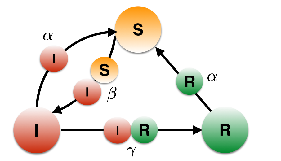
One can represent the states and state transitions of the SIR model with the schematic diagrams in Figs. 1 and 2, where arrows going through pairs of nodes represent reactions that result from interactions, and arrows going through a single node corresponds to a spontaneous transition. We can represent the changing number of S, I, and R individuals through the nonlinear system Eq. 1. Note that population size is constant. Because this will be true of each of the models we study in the paper, we can divide both sides of our differential equations by to obtain equations for the changing fractions , , and within the population. From Section 2 onward, we will consider differential equations in terms of these proportions, but for convenience we will maintain the notation of , , and to represent these fractions.

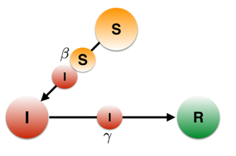
| (1) |
Cannarella and Spechler propose a modification to the traditional SIR model known as “infectious-recovery,” in which an individual’s recovery transition from to does not occur spontaneously, but rather due to an interaction with a recovered individual [3]. In this sense, recovery is itself an infectious process, as recovery is spread through the social interaction of infectious and recovered individuals. The intuition behind this modification is that individuals join OSNs because their real-life friends are also members (the S-I interaction) and then individuals remain members until they see their friends have left (the I-R interaction). In the context of OSN membership, Cannarella and Spechler interpret the susceptible () class to be individuals who have yet to join the OSN, infectious individuals () are active users of the OSN, and recovered () individuals are former users of the OSN. Their infectious-recover SIR (irSIR) model can be represented by the schematic in Fig. 3 or through the system of ODEs in Eq. 2.
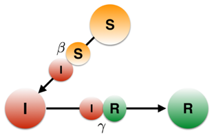
| (2) |
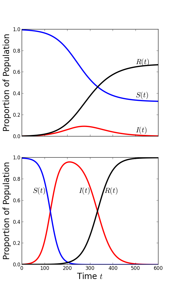
Cannarella and Spechler apply their model to study data from Google Trends for the queries “MySpace” and “Facebook” [3]. Using best-fit techniques, they found parameters for the irSIR model which captured the initial exponential growth and subsequent exponential decay of Google Search interest in MySpace, showing that the irSIR model was more succesful than the SIR model in reproducing the empirical behavior. They apply the same best-fit techniques to search data for Facebook, which has yet to experience a decline similar to MySpace. The paper extrapolated from the best-fit curves to predict that Facebook could lose up to 80 percent of its users in the near future [3].
Several papers have extended the work of Cannarella and Spechler. Fuji uses an asymptotic expansion to find solutions for , , and in the exponential growth phase of the irSIR model [14]. Instead of studying the dynamics of a single OSN in isolation, Tanaka et al consider the takeover of an incumbent social network (users in state ), by a new social network (users in state ). They use Google Trends data to demonstrate that the irSIR model provides a better fit than the SIR model in describing the rise of Facebook’s popularity in Japan at the expense of the incumbent OSN Mixi [15]. Zhu et al study an “irSIRS” model, extending the irSIR model to include demographic terms (corresponding to the creation and deletion of ”bot” accounts) as well as the possibility for recovered individuals to once again become susceptible. They fit their model to user data for the Chinese social networks Renren and Sina-Weibo and predict that the two OSNs will also experience a near-term downturn in active membership [4].
Cintron-Arias uses an epidemic model with an infectious-recovery term to describe the popularity of viral videos. He shows that the model considered exhibits exponential growth for any positive contact rate and validates the model with data of view counts of popular Youtube videos [2]. Ribeiro conducts stability analysis for an OSN model in which active users become inactive due to spontaneous reactions and inactive users can return to active status through interaction with active users [10]. In this model, Ribeiro discovers a phase transition between a regime in which all users ultimately become inactive and one in which a nonzero fraction of users remain active in the long-run.
Here we consider the question of long term behavior for infectious-recovery epidemic models. We show that the long-run behavior of the irSIR model will always result in full abandonment of an OSN. This leads to an interesting question: are there logical extensions of the irSIR model which can result in an asymptotically stable endemic equilbrium? We take inspiration from several biological mechanisms through which a long-run endemic equilibrium can be sustained in extensions of the traditional SIR model: waning immunity and demographic turnover [16]. We show that these reasonable augmentations to the dynamical process of infectious-recovery epidemics lead to dramatic changes in the long time behavior. Characterizing these processes should be helpful for understanding the dynamics of social phenomena and for providing numerical tools to analyze underlying patterns in abundantly available social media data.
The paper is structured as follows. In Section 2, we will analyze Cannarella and Spechler’s original irSIR model through both stability analysis of the system’s equilibria and by evaluating the peak infection size. Then, in Sections 3 and 4, we analyze two extensions of the irSIR model. These extensions are respectively named the irSIRS model with spontaneous loss of immunity (recovered individuals can return to susceptibility on their own), and the demographic irSIR model (in which new susceptibles are introduced to the population at the same rate as individuals of each type are removed).
2. Analysis of irSIR Model
We consider the system
| (3) |
with , , and . We identify points on the simplex of allowed values using the notation .
2.1. Equilibrium Analysis
We begin by reviewing the steady states of the dynamical system. By inspection, all uninfected states (with ) are in equilibrium. Therefore any point with the form for is a fixed point. From the first equation either or must equal 0 if , and either or must equal 0 from the third equation. It follows that the point is the only additional equilibrium. We can represent the three-dimensional system by the two equations
| (4) |
by inserting . The system has Jacobian matrix
At the all-infectious equilibrium , the Jacobian has eigenvalues and , so this equilibrium is unstable. has eigenvalues of and , the latter of which is positive when . Thus equilibria of the form are unstable for , so a small injection of infectious individuals introduced into such a population will result in an initial exponential growth of cases.
2.2. Maximum Number of Infectious Individuals
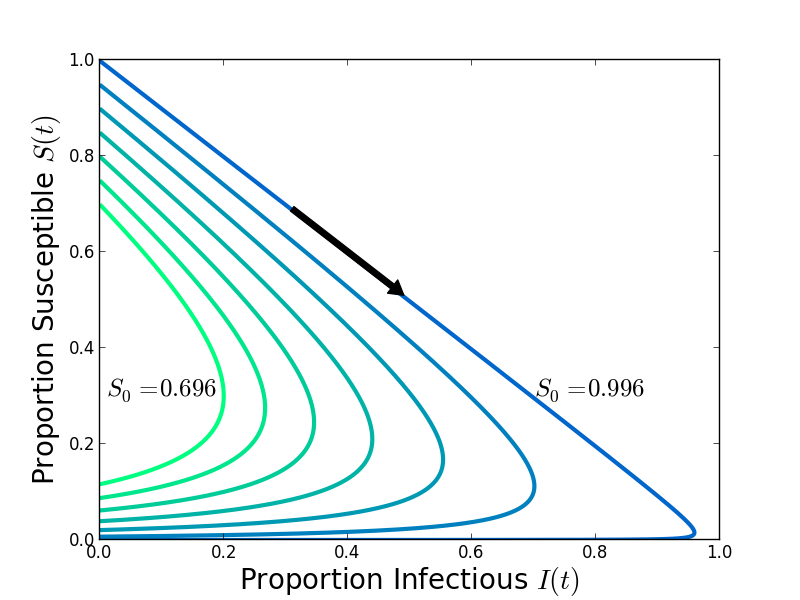
An interesting difference between the irSIR and SIR models is the range of possible values for when the dynamics start from a small perturbation of the disease-free equilibrium. The maximum number of infectious individuals can reach an arbitrarily large proportion of the populations in the irSIR model. This makes the model particularly relevant for applications to internet tools and memes, as, for example, the complete saturation of the population should be a realistic possibility for tools such as email. We show this using Eq. 3 to obtain
so
| (5) |
If , a small results in an initial exponential growth in , which is maximized ( ) when . From Eq. 5 at peak infectiousness ( time ),
| (6) |
On the other hand, if ( for small enough ), we have
for all time and therefore the peak infectiousness will equal . For the SIR model, one can use a similar approach to derive the maximum
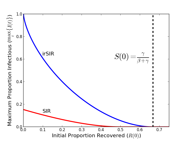
when and otherwise [17]. It follows that the peak infectiousness is achieved at . The values of and are displayed in Fig. 6 for various initial proportions of recovered individuals . For this set of parameter values , , and , we see that and when and when .
We can also obtain the total number of individuals that become infected over the course of the outbreak [17]. Because vanishes in the long run, we obtain the relationship as , so we can numerically solve for by substituting for in Eq. 5. Then subtracting from gives us the total number of individuals that were ever in state at any point in the outbreak.
3. irSIRS Model with Spontaneous Loss of Immunity
We now consider an extension of the irSIR model in which individuals in the removed class can once again become susceptible through a spontaneous reaction (Fig. 7). This models individuals who have left the social network transitioning (without interaction) to a state in which they can be convinced to the rejoin through interaction with an active user. This is given by the set of equations
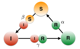
| (7) |
where parameters satisfy and ( corresponds to the irSIR model). There are two equilibria at the corners of the simplex: the disease-free equilibrium and the all infectious equilibrium . If , there is an interior equilbrium
3.1. Local Stability Analysis
For the equilibrium analysis, we use the conservation of population to write
| (8) |
with Jacobian
For the disease-free equilibrium, the Jacobian has
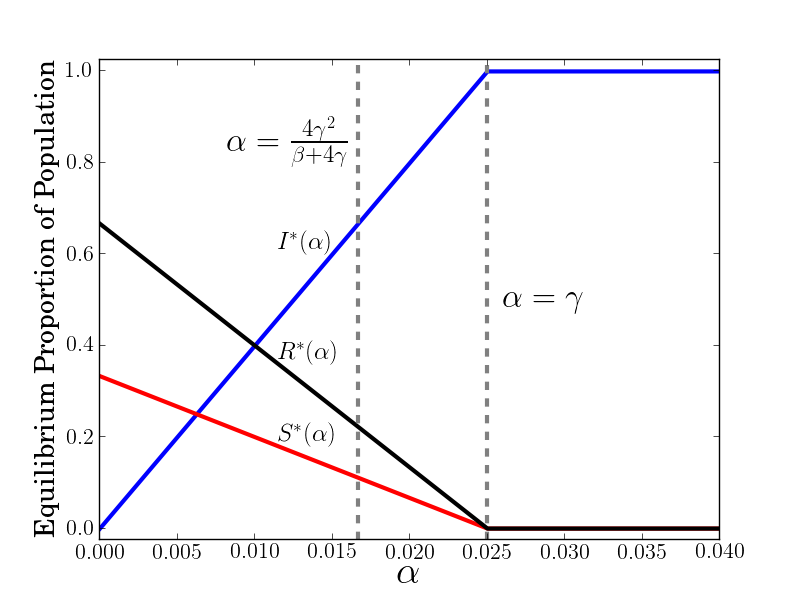
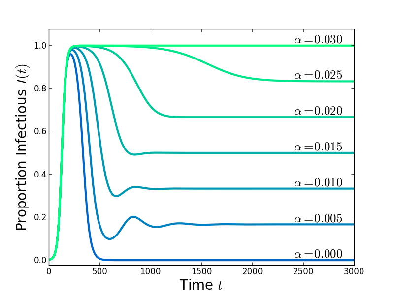
eigenvalues and , so the equilibrium is unstable. For the all-infectious equilibrium, the Jacobian has eigenvalues and , so it is unstable when and stable when . For the interior equilibrium, the Jacobian has eigenvalues . When the discriminant is negative, and thus the interior equilibrium is a stable focus. If , the discriminant is real and less than one, so the interior equilibrium is a stable node. When , the interior equilibrium does not exist, as . Thus the interior equilibrium is always stable when it exists. The value of , , and for the system’s unique stable equilibrium for given is displayed in Fig. 8.
For this model, the initial exponential growth rate is given by (the unstable eigenvalue of the disease-free equilibrium), and then the long-run value of depends only on the relative values of and . By contrast, both the exponential growth rate and long-run limit of depend on and [16], so the irSIRS model is perhaps more capable of separately describing a social phenomenon’s catchiness and staying power.
3.2. Global Stability Analysis
The analysis of the long time dynamical behavior of a system can be clarified by using a theorem of Bendixson and Dulac, who showed that the existence of certain functions (Dulac functions) imply the absense of periodic orbits. We will now use Dulac functions to show that the locally asymptotic equilibria are globally stable on the interior of the simplex, following the techniques of Hethcote [18]. We reduce Eq. 7 to a system in the variables and
| (9) |
We see that is a Dulac function for this system, as
so there are no periodic orbits contained in the interior of the simplex, and we apply the Poincare-Bendixson theorem to conclude that the unique interior equilibrium (for given ) is globally asymptotically stable for initial conditions on the interior of the simplex.
4. irSIR Model with Demography
We extend the irSIR model by considering demographic events that allow new susceptible individuals to be spontaneously introduced to the population and individuals of all types to be spontaneously removed from the population (Fig. 10). In the epidemiological literature, these events correspond to births and deaths, while Zhu et al motivated the use of demographic terms in OSN models by the creation and deletion of bot accounts [4]. One additional motivation for adding demographic terms is that individuals can enter and exit the target demographic class for a particular social network. For example, registration for Facebook once required a “.edu” email address, so the “birth” and “death” terms for such a model could be interpreted as the rates of the matriculation of new (and thereby susceptible) students and the graduation of old students. The system of equations is given by
| (10) |
where parameters satisfy and . We summarize the analysis of equilibria for this system.
4.1. Existence of Equilibria
The system has three equilibria:
-
•
The disease free equilibrium: .
-
•
An equilibrium on the edge of the simplex: which only exists when .
-
•
An interior equilibrium: which exists for and
(11) It follows from Eq. 11 that , so the existence of the interior equilibrium on the simplex implies the existence of the edge equilibrium. To see this, assume . If , then Eq. 11 implies that , which contradicts at least one of or . If , we divide both sides of Eq. 11 by the negative quantity , giving , contradicting .
We can also rewrite the existence condition in Eq. 11 to better represent as a bifurcation parameter as
4.2. Stability Analysis
We use the simplex constraint to reduce our system to
| (12) |
which has Jacobian
For the disease-free equilibrium, the Jacobian has eigenvalues and . so it is asymptotically stable if and only if . The edge equilibrium has eigenvalues
For this equilibrium to be asymptotically stable, we need both that
where all implications follow from , and thus the edge equilibrium is stable when . The interior equilibrium has eigenvalues , so it is asymptotically stable if and only if ,
where we again applied the condition . This inequality is also the condition for the existence for the interior equilibrium, so the equilibrium is stable whenever it exists.
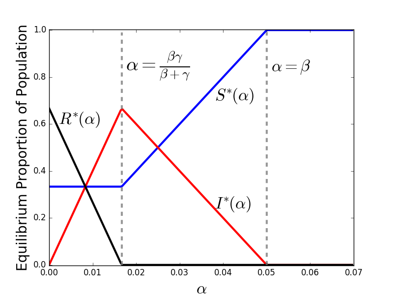
See Fig. 11 for the unique stable equlibrium for given . , the maximum value of at equilibrium for any , is achieved at the bifurcation point . This can also be shown analytically, as we see that increases linearly from to as increases from to (where the interior equilibrium is stable), and then decreases linearly from to as increases from to (where the edge equilibrium is stable). Therefore , and this is achieved for the intermediate demographic rate . Higher or lower demographic turnover produce smaller proportions of long-run infectious in the social epidemic.
Using the Dulac function , we can again use the Bendixson-Dulac criterion to rule out periodic orbits on the interior of the simplex, and we conclude that our unique (for given ) locally stable fixed points are also globally stable for all initial conditions on the simplex.
5. Conclusion
We studied a recently developed class of ODE models for OSN membership that draw inspiration from models in mathematical epidemiology. We used linear stability analysis and peak infection size calculations to characterize the possible behaviors of Cannarella and Spechler’s irSIR model. We also considered two extensions of the irSIR model that describe different social mechanisms by which a long-run stable equilibrium with nonzero OSN membership can be achieved by well-mixed populations, and we derived local and global stability results for these extended models.
In particular, our investigations of the mechanisms of spontaneous loss of immunity and demographic “births” and “deaths” have allowed us to show that even a small perturbation of the equations of the irSIR model may result in a long-run globally stable endemic equilibrium, even though the original irSIR model predicts long-run abandonment. Of note, the irSIRS model with spontaneous return to infection allows for an arbitrary fraction of infectious individuals in the long run population and the irSIR model with demography has a peak level of long run infectiousness at an intermediate level of demographic replacement rate .
The study of the irSIR model and its extensions may also have application to various problems in population dynamics. For example, the coupled terms in the irSIR model bears similarity to generalized Lotka-Volterra model used to describe the ecological dynamics of three species food chains [19, 20, 21]. Exploration of the irSIR model is an interesting exercise because it allows ideas from mathematical epidemiology and nonlinear dynamics to help understand modern human social dynamics, bridging the natural and social sciences and providing inspiration for questions in computer science and the computational social sciences about OSNs and about the spread of social contagion on the internet.
References
- [1] Limor Shifman. Memes in Digital Culture. MIT Press, 2013.
- [2] Ariel Cintron-Arias. To go viral. arXiv preprint arXiv:1402.3499, 2014.
- [3] John Cannarella and Joshua A Spechler. Epidemiological modeling of online social network dynamics. arXiv preprint arXiv:1401.4208, 2014.
- [4] Xiang Zhu, Yuanping Nie, and Aiping Li. Demographic prediction of online social network based on epidemic model. In Web Technologies and Applications, pages 93–103. Springer, 2014.
- [5] Daryl J Daley and David G Kendall. Epidemics and rumours. 1964.
- [6] Romualdo Pastor-Satorras and Alessandro Vespignani. Epidemic spreading in scale-free networks. Phys. Rev. Lett., 86:3200–3203, Apr 2001.
- [7] Rebecca A Jeffs, John Hayward, Paul A Roach, and John Wyburn. Activist model of political party growth. Physica A: Statistical Mechanics and its Applications, 442:359–372, 2016.
- [8] Luís MA Bettencourt, Ariel Cintrón-Arias, David I Kaiser, and Carlos Castillo-Chávez. The power of a good idea: Quantitative modeling of the spread of ideas from epidemiological models. Physica A: Statistical Mechanics and its Applications, 364:513–536, 2006.
- [9] Fang Jin, Edward Dougherty, Parang Saraf, Yang Cao, and Naren Ramakrishnan. Epidemiological modeling of news and rumors on twitter. In Proceedings of the 7th Workshop on Social Network Mining and Analysis, page 8. ACM, 2013.
- [10] Bruno Ribeiro. Modeling and predicting the growth and death of membership-based websites. In Proceedings of the 23rd international conference on World Wide Web, pages 653–664. ACM, 2014.
- [11] Christian Bauckhage. Insights into internet memes. In Fifth International AAAI Conference on Weblogs and Social Media, 2011.
- [12] William O Kermack and Anderson G McKendrick. A contribution to the mathematical theory of epidemics. In Proceedings of the Royal Society of London A: Mathematical, Physical and Engineering Sciences, volume 115, pages 700–721. The Royal Society, 1927.
- [13] Nicola Perra, Duygu Balcan, Bruno Gonçalves, and Alessandro Vespignani. Towards a characterization of behavior-disease models. PloS one, 6(8):e23084, 2011.
- [14] Kazuyuki Fujii. Comment on” epidemiological modeling of online social network dynamics”. Far East Journal of Mathematical Education, 12(2):179, 2014.
- [15] Moena Tanaka, Yusuke Sakumoto, Masaki Aida, and Konosuke Kawashima. Study on the growth and decline of snss by using the infectious recovery sir model. In Information and Telecommunication Technologies (APSITT), 2015 10th Asia-Pacific Symposium on, pages 1–3. IEEE, 2015.
- [16] Matt J Keeling and Pejman Rohani. Modeling infectious diseases in humans and animals. Princeton University Press, 2008.
- [17] Howard Weiss. The sir model and the foundations of public health. In Materials Matemàtics, pages 1–17, 2013.
- [18] Herbert W Hethcote. Qualitative analyses of communicable disease models. Mathematical Biosciences, 28(3):335–356, 1976.
- [19] Erica Chauvet, Joseph E Paullet, Joseph P Previte, and Zac Walls. A lotka-volterra three-species food chain. Mathematics magazine, pages 243–255, 2002.
- [20] Mohammad Hossein Rahmani Doust. An analysis on the lotka-volterra food chain model: Stability. Caspian Journal of Mathematical Sciences, 2014.
- [21] M Mamat, WS Mada Sanjaya, Z Salleh, and MF Ahmad. Numerical simulation dynamical model of three-species food chain with lotka-volterra linear functional response. Journal of Sustainability Science and Management, 6(1):44–50, 2011.