Binary Black Hole merger in $f(R)$ theory

Abstract

In the near future, gravitational wave detection is set to become an important observational tool for astrophysics. It will provide us with an excellent means to distinguish different gravitational theories. In effective form, many gravitational theories can be cast into an $f(R)$ theory. In this article, we study the dynamics and gravitational waveform of an equal-mass binary black hole system in $f(R)$ theory. We reduce the equations of motion in $f(R)$ theory to the Einstein-Klein-Gordon coupled equations. In this form, it is straightforward to modify our existing numerical relativistic codes to simulate binary black hole mergers in $f(R)$ theory. We considered binary black holes surrounded by a shell of scalar field. We solve the initial data numerically using the Olliptic code. The evolution part is calculated using the extended AMSS-NCKU code. Both codes were updated and tested to solve the problem of binary black holes in $f(R)$ theory. Our results show that the binary black hole dynamics in $f(R)$ theory is more complex than in general relativity. In particular, the trajectory and merger time are strongly affected. Via the gravitational wave, it is possible to constrain the quadratic part parameter of $f(R)$ theory in the range $|a_{2}|<10^{11}$m². In principle, a gravitational wave detector can distinguish between a merger of binary black hole in $f(R)$ theory and the respective merger in general relativity. Moreover, it is possible to use gravitational wave detection to distinguish between $f(R)$ theory and a non self-interacting scalar field model in general relativity.

I introduction

Einstein’s general relativity (GR) is currently the most successful gravitational theory. It has excellent agreement with many experiments (see e.g. Wil06 ; Sta03 ; Ash03 ). However, most of the tests involve weak gravitational fields. On the other hand, recent cosmological observations require ad-hoc explanations to fit in the framework of GR theory, for example the dark energy and dark matter problems Hut10 ; CopSamTsu06 ; LiLiWan11 . In order to solve these difficulties, some alternative gravitational theories have been proposed JaiKho10 ; SilTro09 .

In effective form, many gravitational theories can be caste into an $f(R)$ theory FelTsu10 ; SotFar10 ; HuaLiMa10 ; ZhaMa11 ; ZhaMa11a . Additionally, $f(R)$ theory has a relatively simple form. Therefore, it is a good alternative gravitational model. In this work, we characterize the gravitational waveform of binary black hole mergers in $f(R)$ theory.

In the near future, gravitational wave detection will become an observational method for astrophysics AbrAltAre92 ; BraFabVir90 ; Mag00 ; GonXuBai11 . The gravitational wave experiments can be excellent tools for testing GR in strong field regime. Moreover, it will be possible to distinguish different gravitational theories. Quantitatively, future experimental data can be used to constrain $f(R)$ parameters, and to confirm or to reject alternative gravitational theories. With this in mind, we analyze the waveforms in order to quantify the differences. According to our results, it is possible to distinguish quadratic models of $f(R)$ and GR with future experimental data.

The quadratic form of $f(R)$ is given by $f(R)=R+a_{2}R^{2}$. The main free parameter is the coefficient of the quadratic part $a_{2}$. In the case $a_{2}=0$, $f(R)$ theory reduces to GR. In linearized $f(R)$ it is possible to shows that Mercury’s orbit sets the value of $|a_{2}|\leq 1.2\times 10^{18}\,\mathrm{m}^{2}$ BerGai11 . On the other hand, Eöt-Wash experiments restrict the value of $|a_{2}|\leq 2\times 10^{-9}\,\mathrm{m}^{2}$ HoyKapHec04 ; KapCooAde07 . The Laser Interferometer Space Antenna (LISA) may distinguish $|a_{2}|\geq 10^{17}\,\mathrm{m}^{2}$. Binary black holes in the mass range $30-300\,M_{\mathrm{sun}}$ are expected to merge at frequencies in the most sensitive region of the Laser Interferometer Gravitational Wave Observatory (LIGO) frequency band VaiHinSho09 . Therefore, we focused our attention on an equal-mass binary black hole system with total mass $M=m_{1}+m_{2}=100\,M_{\mathrm{sun}}$. We find that the LIGO detection can distinguish $|a_{2}|\geq 10^{11}\,\mathrm{m}^{2}$.

The paper is organized as follows: in Sec. II, we summarize the equations of $f(R)$ theory. This is followed by a description of the initial data setup in Sec. III. In Sec. IV.1, we describe the numerical techniques used to solve the equations of motion. In Sec. IV.2, we give some motivation and background for the configuration used in this work. The evolution of equal-mass binary black hole system is presented in Sec. IV.3. Conclusions and discussions are presented in Sec. V.

I.1 Notation and units

We employ the following notation: Space-time indices take values between 0 and 3, with 0 representing the time coordinate. The first Latin indices $(a,b,c,\dots,h)$ refer to four-dimensional space-time and take values between 0 and 3, while Latin indices $(i,j,k,l,\dots)$ refer to three-dimensional space and take values from 1 to 3. The metric signature is $(-1,1,1,1)$. Some references (e.g., BerGai11 ), use a metric signature $(1,-1,-1,-1)$. The difference is a change of sign of the scalar curvature $R$ as well as $f(R)$. We use Einstein’s summation convention. The symbol $a:=b$ means that $a$ is defined as being b. A dot over a symbol, $\dot{\vec{x}}$, means the total time derivative, and partial differentiation with respect to $x^{i}$ is denoted by $\partial_{i}$. Differentiation with respect to the Ricci scalar $R$ is denoted with a prime, for example $f^{\prime}:=\frac{df(R)}{dR}$.

In order to simplify the calculations, we use geometric units, where the speed of light $c$ and the gravitational constant $G$ are normalized to 1. A variable in bold font, i.e. $\mathbf{x}$, denotes physical quantities in international system units. Particularly, the values of $a_{2}\approx 1\,\mathrm{M}^{2}$ in geometric units corresponds to $\mathbf{a_{2}}\approx 10^{11}\mathrm{m}^{2}$ for typical gravitational wave sources of binary black hole for LIGO.

We use the following abbreviations: Einstein’s general relativity (GR), Laser Interferometer Space Antenna (LISA), Laser Interferometer Gravitational Wave Observatory (LIGO), Einstein-Klein-Gordon (EKG), Baumgarte-Shapiro-Shibata-Nakamura (BSSN), Arnowitt-Deser-Misner (ADM) and binary black hole (BBH).

II Mathematical background

In vacuum spacetimes, $f(R)$ theory generalizes the Hilbert-Einstein action to

$$S=\int\frac{d^{4}x}{16\pi}\sqrt{-g}f(R),$$ (1)

where GR is recovered by setting $f(R)=R$. From this action, we obtain the Euler-Lagrange equations of motion

$$f^{\prime}R_{ab}-\frac{1}{2}fg_{ab}-[\nabla_{a}\nabla_{b}-g_{ab}\Box]f^{\prime}=0.$$ (2)

Using the definition of Einstein tensor $G_{ab}:=R_{ab}-g_{ab}R/2$, we obtain after subtracting a Ricci tensor term $Rg_{ab}/2$ in (2), and rearranging terms,

$$G_{ab}=\frac{1}{f^{\prime}}\left[\nabla_{a}\nabla_{b}f^{\prime}-g_{ab}\Box f^{\prime}-\frac{1}{2}g_{ab}\left(Rf^{\prime}-f\right)\right].$$ (3)

On the other hand, considering the conformal transformation $\tilde{g}_{ab}=e^{2\omega}g_{ab}$, the Ricci tensor transforms into

$$\tilde{R}_{ab}=R_{ab}-$$

$$2\nabla_{a}\nabla_{b}\omega-g_{ab}\Box\omega+2\nabla_{a}\omega\nabla_{b}\omega-2g_{ab}g^{de}\nabla_{d}\omega\nabla_{e}\omega.$$ (4)

The corresponding Ricci scalar transforms as

$$\tilde{R}=e^{-2\omega}\left(R-6\Box\omega-6g^{de}\nabla_{d}\omega\nabla_{e}\omega\right).$$ (5)

Therefore, the Einstein tensor transformation is given by

$$\tilde{G}_{ab}=G_{ab}-$$

$$2\nabla_{a}\nabla_{b}\omega+2g_{ab}\Box\omega+2\nabla_{a}\omega\nabla_{b}\omega+g_{ab}g^{de}\nabla_{d}\omega\nabla_{e}\omega.$$ (6)

Defining $\omega:=\frac{1}{2}\ln\lambda$, we have

$$\nabla_{a}\omega= \frac{1}{2\lambda}\nabla_{a}\lambda,$$ (7)

$$\nabla_{a}\nabla_{b}\omega= -\frac{1}{2\lambda^{2}}\nabla_{a}\lambda\nabla_{b}\lambda+\frac{1}{2\lambda}\nabla_{a}\nabla_{b}\lambda.$$ (8)

The substitution of (7) and (8) in (6) implies

$$\tilde{G}_{ab}= G_{ab}+\frac{3}{2\lambda^{2}}\nabla_{a}\lambda\nabla_{b}\lambda-\frac{3}{4\lambda^{2}}g_{ab}g^{de}\nabla_{d}\lambda\nabla_{e}\lambda$$

$$-\frac{1}{\lambda}\left(\nabla_{a}\nabla_{b}\lambda-g_{ab}\Box\lambda\right).$$ (9)

Substituting $\lambda:=f^{\prime}$ in (3) and the result in (9), we get

$$\tilde{G}_{ab}=\frac{3}{2\lambda^{2}}\nabla_{a}\lambda\nabla_{b}\lambda-\frac{3}{4\lambda^{2}}g_{ab}g^{de}\nabla_{d}\lambda\nabla_{e}\lambda-\frac{\left(R\lambda-f\right)}{2\lambda}g_{ab}.$$ (10)

Since the conformal transformation satisfies $\tilde{g}_{ab}=\lambda g_{ab}$, (10) takes the form

$$\tilde{G}_{ab}=\frac{3}{2\lambda^{2}}\tilde{\nabla}_{a}\lambda\tilde{\nabla}_{b}\lambda-\frac{3}{4\lambda^{2}}\tilde{g}_{ab}\tilde{g}^{de}\tilde{\nabla}_{d}\lambda\tilde{\nabla}_{e}\lambda-\frac{\left(R\lambda-f\right)}{2\lambda^{2}}\tilde{g}_{ab}.$$ (11)

Defining $\phi:=\sqrt{\frac{3}{16\pi}}\ln\lambda$, we get

$$\tilde{G}_{ab}=8\pi\left[\tilde{\nabla}_{a}\phi\tilde{\nabla}_{b}\phi-\tilde{g}_{ab}\left(\frac{1}{2}\tilde{g}^{de}\tilde{\nabla}_{d}\phi\tilde{\nabla}_{e}\phi+V\right)\right].$$ (12)

where

$$V:=\frac{R\mathrm{e}^{4\sqrt{\pi/3}\phi}-f}{16\pi\mathrm{e}^{8\sqrt{\pi/3}\phi}}.$$ (13)

The right hand side of (12) has the form of the stress energy tensor of a scalar field (see e.g. Wal84 ; Car03 )

$$\tilde{T}_{ab}:=\tilde{\nabla}_{a}\phi\tilde{\nabla}_{b}\phi-\tilde{g}_{ab}\left(\frac{1}{2}\tilde{\nabla}_{c}\phi\tilde{\nabla}^{c}\phi+V\right).$$ (14)

Therefore, in vacuum, the $f(R)$ theory equations of motion are equivalent to GR equations coupled to a real scalar field

$$\phi=\frac{\sqrt{3}}{4\sqrt{\pi}}\ln f^{\prime}.$$ (15)

The equation of motion of the scalar field is given by the trace of (2) with $g^{ab}$

$$\tilde{\square}f^{\prime}=2\tilde{\nabla}^{a}\omega\tilde{\nabla}_{a}f^{\prime}-\frac{2f-f^{\prime}R}{3},$$ (16)

where we have employed the conformal metric transformation. Substituting the definition of $\phi$ we get

$$\tilde{\square}\phi =\frac{2f-f^{\prime}R}{4\sqrt{3\pi}f^{\prime 2}}$$

$$=\frac{2f-Rf^{\prime}}{16\pi f^{\prime 3}}f^{\prime\prime}\frac{dR}{d\phi}$$

$$=\frac{dV}{d\phi}.$$ (17)

The result is the dynamical equation of a real scalar field with potential $V$. Therefore, the equations of motion for $f(R)$ theory are equivalent to Eqs. (12) and (17), which form the EKG system of equations. Notice that the scalar field is introduced for numerical simulation convenience. Moreover, it is related to the Ricci scalar. Therefore, it does not represent a physical freedom.

The equations of motion derived with the metric $\tilde{g}_{ab}$ are commonly referred to be in the Einstein frame. For physical interpretation, we need to transform them using the physical metric $g_{ab}=e^{-4\sqrt{\frac{\pi}{3}}\phi}\tilde{g}_{ab}$. The equations in that form are referred to be in the Jordan frame. We use Newman-Penrose scalar $\Psi_{4}$ to analyze gravitational waveform. Therefore, it is calculated through $\tilde{\Psi}_{4}=e^{-4\sqrt{\frac{\pi}{3}}\phi}\Psi_{4}$. Since the Weyl tensor is conformal invariant, the pre-factor comes from a tetrad transformation.

We use 3+1 formalism to solve (12) and (17). For Einstein equations (12) we adopt the BSSN formulation as in our previous work CaoYoYu08 . The scalar field equations (17) can be decomposed using the 3+1 formalism as follows (see e.g., for detail about the 3+1 formalism Alc08 ; Gou12 ): First it is useful to define an auxiliary variable $\varphi:=\mathcal{L}_{\mathbf{n}}\phi$, where $\mathcal{L}_{\mathbf{n}}$ denotes the Lie derivative along the normal to the hypersurface $\Sigma_{t}$. Expressing the Lie derivative in terms of the lapse function $\alpha$ and the shift vector $\beta^{i}$, the evolution of $\phi$ is given by

$$\partial_{t}\phi=\alpha\varphi+\beta^{i}\partial_{i}\phi.$$ (18)

On the other hand, the evolution of $\varphi$ is given by the substitution of $\mathcal{L}_{\mathbf{n}}\phi$ in (17)

$$\partial_{t}\varphi =\alpha\chi\left(\bar{\gamma}^{ij}\partial_{i}\partial_{j}\phi-(\bar{\Gamma}^{i}+\frac{\bar{\gamma}^{ij}\partial_{j}\chi}{2\chi})\partial_{i}\phi\right)+\chi\bar{\gamma}^{ij}\partial_{i}\alpha\partial_{j}\phi$$

$$+\alpha\varphi K-\alpha\frac{dV}{d\phi}+\beta^{i}\partial_{i}\varphi,$$ (19)

where we used the BSSN metric conformal transformation $\bar{\gamma}_{ij}=\chi\gamma_{ij}$ and the relationships

$$K =-\frac{\gamma^{ij}}{2\alpha}\frac{\partial\gamma_{ij}}{\partial t},$$ (20)

$$\Gamma^{i} =-\frac{1}{\sqrt{\gamma}}\partial_{j}\left(\sqrt{\gamma}\gamma^{ij}\right),$$ (21)

with $K$ the trace of the extrinsic curvature, $\gamma$ the determinant of the 3-metric and $\Gamma^{i}$ the contracted Christoffel symbol. The quantities with an upper bar are represented in the conformal metric of BSSN form.

The matter densities are given by

$$E :=n_{a}n_{b}T^{ab}$$

$$=\frac{1}{2}D_{i}\phi D^{i}\phi+\frac{1}{2}\varphi^{2}+V,$$ (22)

$$p_{i} :=-\gamma_{ia}n_{b}T^{ab}$$

$$=-\varphi D_{i}\phi,$$ (23)

$$S_{ij} :=\gamma_{ia}\gamma_{jb}T^{ab}$$

$$=D_{i}\phi D_{j}\phi-\gamma_{ij}\left(\frac{1}{2}D_{k}\phi D^{k}\phi-\frac{1}{2}\varphi^{2}+V\right).$$ (24)

For $f$, we consider a quadratic form $f(R)=R+a_{2}R^{2}$, which results in the potential

$$V=\frac{1}{32\pi a_{2}}(1-e^{4\sqrt{\pi/3}\phi})^{2}e^{-8\sqrt{\pi/3}\phi}.$$ (25)

This potential is analytic around $\phi=0$ and it can be expanded as

$$V=\frac{1}{6a_{2}}{\phi}^{2}-\frac{2}{3a_{2}}\sqrt{\frac{\pi}{3}}{\phi}^{3}+{\frac{14\pi}{27a_{2}}}{\phi}^{4}-\frac{8\pi}{9a_{2}}\sqrt{\frac{\pi}{3}}{\phi}^{5}+O\left({\phi}^{6}\right).$$ (26)

The coefficient of $\phi^{2}$ is related to the mass of the scalar field ($m=1/\sqrt{6a_{2}}$) and the other terms imply that the scalar field has nonlinear self-interaction. With the signature convention taken in this work, only the positive values of $a_{2}$ are physically meaningful. Therefore, we demand that $a_{2}\geq 0$.

II.1 Formalism for numerical calculation of $f(R)$ dynamics

The dynamical equations for $f(R)$ theory can be written as (2), or equivalently as (12). There is a key component in BSSN formalism where $\bar{\Gamma}^{i}$ are consider to be new independent functions. Similar to this, we promote $\phi$ to a new independent function. Then the evolution equation of $\phi$ is determined by (17). On the other hand, the definition of $\phi$ (15 is a constraint equation. For later reference, we summarize the equations for numerical calculation of $f(R)$ dynamics as follows

$$\tilde{G}_{ab} =8\pi\tilde{T}_{ab},$$ (27)

$$\tilde{\square}\phi =\frac{dV}{d\phi}.$$ (28)

The constraint equation is

$$\ln f^{\prime}=\frac{4\sqrt{\pi}}{\sqrt{3}}\phi.$$ (29)

It is interesting to note that the original dynamical equation (2) for $f(R)$ theory includes 4th order derivative terms of metric. This is because $f$ depends on $R$, which contains second derivative terms of the metric, and (2) contains second derivative terms of $f$. After performing a conformal transformation, we obtain the dynamical equation (12). If we look at the conformal metric $\tilde{g}_{ab}$ instead of $g_{ab}$ as dynamical variables, (12) involves 3rd order derivatives which come from the derivative of $\phi$. This is because $\phi$ itself is a function of $R$ which contains second derivative of conformal metric. In (27) and (28), we replace the 3rd order derivative terms by promoting the auxiliary variable $\phi$ as an independent variable. This treatment introduces an extra constraint equation (29) which is similar to the role of the Gamma constraint equations in BSSN numerical scheme. With this treatment, equations (27) and (28) contain at most second order derivative terms.

The system of equations (27) and (28) takes the form of coupled Einstein-Klein-Gordon equations. For Einstein equation we use the BSSN formulation. We monitor the constraint equation (29) to check the consistency of our numerical solutions.

III Initial Data

Under a 3+1 decomposition, the constraint equations read as follows:

$$D_{j}K^{j}{}_{i}-D_{i}K =8\pi p_{i},$$ (30)

$$R+K^{2}-K_{ij}K^{ij} =16\pi E,$$ (31)

where $R$ is the Ricci scalar, $K_{ij}$ is the extrinsic curvature, $K$ the trace of the extrinsic curvature, $\gamma_{ij}$ the 3-metric, and $D_{j}$ the covariant derivative associated with $\gamma_{ij}$. $E$ and $p_{i}$ are the energy and momentum densities given in equations (22) and (23).

III.1 Puncture method

The constraints can be solved with the puncture method BraBru97 . Following the conformal transverse-traceless decomposition approach, we make the following assumptions for the metric and the extrinsic curvature:

$$\gamma_{ij}=\psi_{0}^{4}\hat{\gamma}_{ij},$$ (32)

$$K_{ij}=\psi_{0}^{-2}\hat{A}_{ij}+\frac{1}{3}K\hat{\gamma}_{ij},$$ (33)

where $\hat{A}_{ij}$ is trace free and $\psi_{0}$ is a conformal factor. We chose a conformally flat background metric, $\hat{\gamma}_{ij}=\delta_{ij}$, and a maximal slice condition, $K=0$. The last choice decouples the constraint equations (30)-(31) to take the form

$$\partial_{j}\hat{A}^{ij}=0,$$ (34)

$$\vartriangle\psi_{0}+\frac{1}{8}\hat{A}^{ij}\hat{A}_{ij}\psi_{0}^{-7}=-\psi_{0}\delta^{ij}\partial_{i}\phi\partial_{j}\phi-2\pi\psi_{0}^{5}V,$$ (35)

where $\vartriangle$ is the Laplacian operator associated with Euclidian metric. Notice that we have chosen $\varphi\equiv\mathcal{L}_{\mathbf{n}}\phi=0$ initially. This is consistent to the quasi-equilibrium picture. So $p_{i}=0$ which results in (34).

In a Cartesian coordinate system $(x^{i})=(x,y,z)$, there is a non-trivial solution of (34) which is valid for any number of black holes BowYor80 (here the index $n$ is a label for each puncture):

$$\hat{A}^{ij} = \sum_{n}\left[\frac{3}{2r^{3}_{n}}\left[x_{n}^{i}P_{n}^{j}+x_{n}^{j}P_{n}^{i}-\left(\delta^{ij}-\frac{x_{n}^{i}x_{n}^{j}}{r_{n}^{2}}\right)P^{n}_{k}x_{n}^{k}\right]\right.$$

$$\left.+\frac{3}{r_{n}^{5}}\left(\epsilon^{ik}_{\;\;l}S^{n}_{k}x_{n}^{l}x_{n}^{j}+\epsilon^{jk}_{\;\;l}S^{n}_{k}x_{n}^{l}x_{n}^{i}\right)\right],$$ (36)

where $r_{n}:=\sqrt{(x-x_{n})^{2}+(y-y_{n})^{2}+(z-z_{n})^{2}}$, $\epsilon^{ik}_{\;\;l}$ is the Levi-Civita tensor associated with the flat metric, and $P_{n}$ and $S_{n}$ are the ADM linear and angular momentum of $n$th black hole, respectively.

The Hamiltonian constraint (35) becomes an elliptic equation for the conformal factor $\psi_{0}$. The solution splits as a sum of a singular term and a finite correction $u$ BraBru97 ,

$$\psi_{0}=1+\sum_{n}\frac{m_{n}}{2r_{n}}+u,$$ (37)

with $u\rightarrow 0$ as $r_{n}\rightarrow\infty$. The function $u$ is determined by an elliptic equation on $\mathbb{R}^{3}$, which is derived from (35) by inserting (37), and $u$ is $C^{\infty}$ everywhere except at the punctures, where it is $C^{2}$. The parameter $m_{n}$ is called the bare mass of the $n$th puncture.

III.2 Numerical Method

The Hamiltonian constraint (35) is solved numerically using the Olliptic code (GalBruCao10a ). Olliptic is a parallel computational code which solves three dimensional systems of nonlinear elliptic equations with a 2nd, 4th, 6th, and 8th order finite difference multigrid method Bra77 ; BaiBra87 ; BraLan88 ; HawMat03 ; ChoUnr86b . The elliptic solver uses vertex-centered stencils and box-based mesh refinement.

The numerical domain is represented by a hierarchy of nested Cartesian grids. The hierarchy consists of $L+G$ levels of refinement indexed by $l=0,\ldots,L+G-1$. A refinement level consists of one or more Cartesian grids with constant grid-spacing $h_{l}$ on level $l$. A refinement factor of two is used such that $h_{l}=h_{G}/2^{|l-G|}$. The grids are properly nested in that the coordinate extent of any grid at level $l>G$ is completely covered by the grids at level $l-1$. The level $l=G$ is the “external box” where the physical boundary is defined. We used grids with $l<G$ to implement the multigrid method beyond level $l=G$.

For the outer boundary, we required an inverse power fall-off condition,

$$u(r)=A+\frac{B}{r^{q}},\quad\mathrm{for}\quad r\gg 1,\;q>0,$$ (38)

where the factor $B$ is unknown. It is possible to get an equivalent condition which does not contain $B$ by calculating the derivative of (38) with respect to $r$, solving the equation for $B$ and making a substitution in the original equation. The result is a Robin boundary condition:

$$u(\vec{x})+\frac{r}{q}\frac{\partial u(\vec{x})}{\partial r}=A.$$ (39)

For the initial data, we set $q=1$ and $A=0$.

III.3 Results

III.3.1 Test problem

As a test, we set the mass parameter of the black hole to zero and consider a spherical symmetric field $\phi$ and potential $V$. The Hamiltonian constraint (35) reduces to a second order ordinary differential equation

$$r\psi_{0}^{\prime\prime}+2\psi_{0}^{\prime}+\pi\psi_{0}(\phi^{\prime})^{2}+2\pi V(r)\psi^{5}_{0}=0,$$ (40)

where the prime denotes differentiation with respect to $r$. In order to obtain a high-resolution reference solution, we solve (40) using Mathematica Wol08 . A useful transformation for the case $V=0$ is $\psi_{1}:=r\psi_{0}$. Under this transformation, regularity at the origin implies $\lim_{r\rightarrow 0}\psi_{1}(r)=0$. The boundary condition (39) with $q=1$ and $A=1$ reduces to $\psi_{1}^{\prime}(r_{\mathrm{max}})=1$, where $r_{\mathrm{max}}$ is the radius of our numerical domain. The problem then becomes

$$\psi_{1}^{\prime\prime}+\pi\psi_{1}(\phi^{\prime})^{2}+2\pi V(r)\frac{\psi^{5}_{1}}{r^{4}} =0,$$ (41)

$$\psi_{1}(0) =0,$$ (42)

$$\psi_{1}^{\prime}(r_{\mathrm{max}}) =1.$$ (43)

For the case $V\neq 0$, the term $r^{-4}$ produces a singularity at the origin. We cure artificially the singularity by solving the equation with a term $(r^{4}+\epsilon)^{-1}$ instead of $r^{-4}$. For the test, the value of $\epsilon$ is set to $10^{-12}$.

We considered 2 cases

$$\begin{array}[]{ll}\mathrm{Case\quad I:}&\phi(r)=\phi_{0}\tanh[(r-r_{0})/\sigma],\\ &V(r)=0.\\ \mathrm{Case\quad II:}&\phi(r)=\phi_{0}\mathrm{e}^{-(r-r_{0})^{2}/\sigma},\\ &V(r)=\frac{1}{32\pi a_{2}}\left(1-\mathrm{e}^{4\sqrt{\pi/3}\phi}\right)^{2}\mathrm{e}^{-8\sqrt{\pi/3}\phi},\end{array}$$

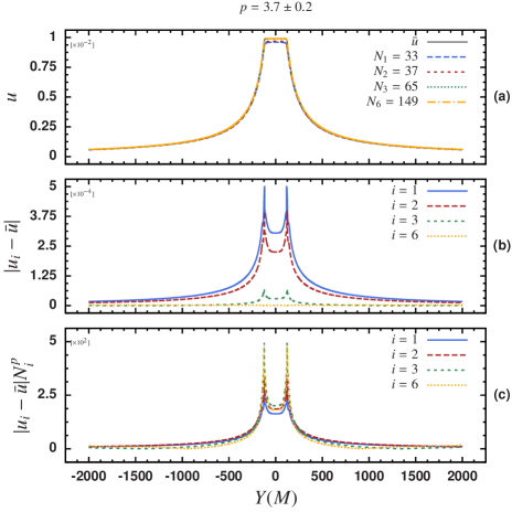
where in both cases $r_{0}=120M$, $\sigma=8M$, $\phi_{0}=1/40$. For case II, we set $a_{2}=1$. The numerical domain is a cubic box of size 4000 ($r_{\mathrm{max}}=2000$) and 11 refinements levels. We use the fourth order finite difference stencil since it provides a good convergence property at the boundary for large domains (see GalBruCao10a for details). The convergence tests consist of a set of six solutions with grid points $N_{i}\in\{43,51,75,105,129,149\}$. The comparison with the reference solution was performed along the $Y$ axis using a 6th order Lagrangian interpolation. For each resolution, the difference $E_{i}:=|u_{i}-\bar{u}|$ gives an estimation of the error. Here $u_{i}$ denotes the solution produced with Olliptic, $i$ is an index which labels the grid size, $\bar{u}$ the reference solution and $|\cdot|$ the absolute value (computed point by point). The functions are interpolated in a domain with grid size $\Delta y=1$. The error satisfies $E_{i}\sim Ch_{i}^{p}$, where $C$ is a constant, $h_{i}\sim 1/N_{i}$ is the grid size and $p$ the order of convergence. Using the $L_{1}$ norm of the error and performing a linear regression of $\ln|E_{i}|_{L_{1}}$ vs $\ln|h_{i}|$, we estimate the convergence order $p$ and the constant $C$.

Figure 1 shows the result of case I. There is a good agreement between the several resolutions and the reference solution. The plot does not show noticeable differences (see Fig. 1-(a)). The solution has convergence properties, and the estimated error diminishes with increased resolution (Fig. 1-(b)). The scaled error $E_{i}/h_{i}^{p}$ also shows good convergence with convergence order $p=3.7\pm 0.2$ given by linear regression (Fig. 1-(c)).

Figure 1: Initial data convergence test for case I. The upper panel (a), shows the reference solution and 4 solutions computed with Olliptic . The middle panel (b), presents the estimated error. The lower panel (c), shows the scaled error for convergence order $p=3.7\pm 0.2$.

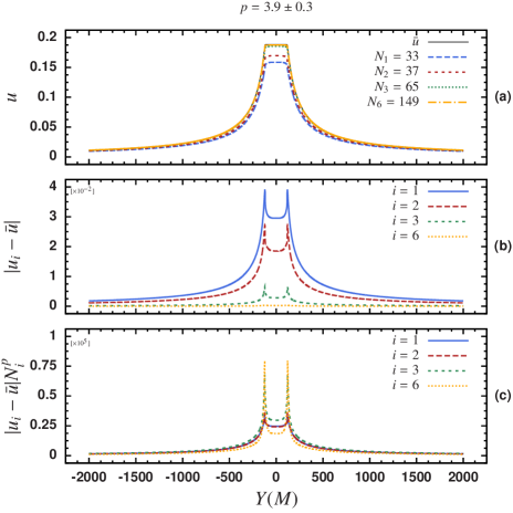
The results for case II are presented in Figure 2. The solution is similar to case I, an almost constant solution between 0 and $r_{0}$ which joins a inverse power solution after $Y=r_{0}$. However, the solution of case II is around 2 orders of magnitude larger than the solution of case I. Contrary to case I, there are noticeable differences between the reference solution and the lower-resolution ones (Fig. 2-(a)). The solution shows convergence properties and the scaled error shows convergence consistently with $p=3.9\pm 0.3$ (Fig. 2-(b),(c)).

Figure 2: Initial data convergence test for case II. The upper panel (a), shows the reference solution and 4 solutions computed with Olliptic . The middle panel (b), presents the estimated error. The lower panel (c), shows the scaled error for convergence order $p=3.9\pm 0.3$.

III.3.2 Initial data for evolution

The solution of (35) provides initial data for our evolutions. The initial parameters of the BBH are: puncture mass parameter $m_{1}=m_{2}=0.487209$ (approximate apparent horizon mass equals to 0.5), initial position $(x,y,z)=(0,\pm 5.5,0)$ and linear momentum $(p_{x},p_{y},p_{z})=(\mp 0.0901099,\mp 0.000703975,0)$. The linear momentum parameter is tuned for non-spinning quasi-circular orbits in GR.

Table 1: ADM mass as function of $\phi_{0}$ for $a_{2}\rightarrow\infty$ (Fig. 3). The values are well represented by a quadratic function $M_{\mathrm{ADM}}=A+B\phi_{0}^{2}$ with $A=0.99067$ and $B=40569\pm 48$.

#	$\phi_{0}$	$M_{\mathrm{ADM}}$	#	$\phi_{0}$	$M_{\mathrm{ADM}}$
1	0	0.990669	7	0.004	1.632418
2	0.0001	0.991069	8	0.005	1.994890
3	0.0005	1.000670	9	0.006	2.439376
4	0.001	1.030680	10	0.007	2.966764
5	0.002	1.150790	11	0.008	3.578118
6	0.003	1.351237	12	0.009	4.274675

Table 2: ADM mass as function of $a_{2}$ (Fig. 4). The value of the maximum (# 8) is estimated using the minimization of (46). The parameter $\phi_{0}$ of the scalar field is $0.001642$.

#	$a_{2}$	$M_{\mathrm{ADM}}$	#	$a_{2}$	$M_{\mathrm{ADM}}$
1	0	9.906691	9	4	1.153111
2	0.2	9.930327	10	6	1.140796
3	0.4	1.006901	11	8	1.132395
4	0.6	1.033066	12	10	1.126691
5	0.8	1.063929	13	20	1.113947
6	1	1.092333	14	40	1.106991
7	2	1.155675	15	60	1.104598
8	2.64791	1.160240	16	80	1.103388

For the scalar field part, we consider that the BBH is surrounded by a shell of scalar field with initial profile

$$\phi(r)=\frac{a_{2}^{2}}{a_{2}^{2}+1}\phi_{0}e^{-(r-r_{0})^{2}/\sigma},$$ (44)

with $r_{0}=120M$, $\sigma=8M$ and several values of $\phi_{0}$ (see below). When $a_{2}$ goes to zero, both $\phi$ and $V$ go to zero. Therefore, standard general relativity is recovered. On the other hand, when $a_{2}\rightarrow\infty$, the amplitude of the scalar field tends to $\phi_{0}$ while the potential vanishes. Our model provides an unified scheme to investigate standard GR ($a_{2}=0$), usual $f(R)$ ($0<a_{2}<\infty$) and the free EKG system in GR ($a_{2}\rightarrow\infty$).

From the solution of the conformal factor it is possible to estimate the ADM mass through

$$M_{\mathrm{ADM}}|_{r=r_{0}}=-\frac{1}{2\pi}\oint_{S}\partial_{j}\psi\;\mathrm{d}S^{j},$$ (45)

where the integration is performed in a sphere $S$ of radius $r_{0}$ (formally the ADM mass is computed taking the limit $r_{0}\rightarrow\infty$). In our calculations $r_{0}=1537.5$ and the integrations is done numerically using 6th order Lagrange interpolation in the sphere and 6th order Boole’s quadrature PreFlaTeu92a ; KarKir03 .

Figure 3: ADM mass $M_{\mathrm{ADM}}$ as function of $\phi_{0}$ for $a_{2}\rightarrow\infty$. The functional behavior is well represented by a quadratic function.

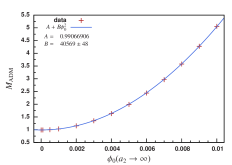
The estimation of the ADM mass gives us a way to analyze the parameters $\phi_{0}$ and $a_{2}$. On one hand, it is possible to compute $M_{\mathrm{ADM}}$ for the case $a_{2}\rightarrow\infty$ for several values of $\phi_{0}$ (see Table 1). The result is a quadratic relationship (see figure 3). The quadratic behavior is consistent with the fact that the coefficient of $\psi_{0}$ in (35) for the scalar field profile (44) is quadratic in the amplitude $\phi_{0}$.

Figure 4: ADM mass $M_{\mathrm{ADM}}$ as function of $\log(a_{2})$. The amplitude of the scalar field is $\phi_{0}=0.001642$. The cross-circle symbol denotes the maximum value $M_{\mathrm{ADM}}=1.16023966$ located at $a_{2}=2.64353$. The value of $a_{2}$ is estimated from the maximization of (46).

Figure 5: Estimated values of $(\phi_{0},a_{2})$ which maximize $M_{\mathrm{ADM}}$. The upper panel (a)  shows the result in the variables $(\tilde{\phi}_{0},\tilde{a}_{2})$, where we fit a second order polynomial. The lower panel (b)  shows the result in the variables $(\phi_{0},a_{2})$. Notice that in both cases the behavior seems to be linear, however by using a linear fit in the tilde variables the result does not fit the data in the $(\phi_{0},a_{2})$ (dashed line).

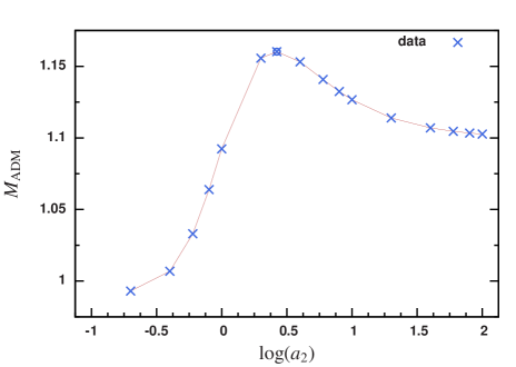
On the other hand, for fixed $\phi_{0}$, we analyzed the functional behavior of $M_{\mathrm{ADM}}$ as function of $a_{2}$. Figure 4 shows the result (in this example $\phi_{0}=0.001642$). For this particular value of $\phi_{0}$, the ADM mass reaches its maximum value $M_{\mathrm{ADM}}=1.16023966$ when $a_{2}=2.64353$. The estimation of the value $a_{2}$ comes from the maximization of the product of the coefficients of $\psi_{0}$ and $\psi_{0}^{5}$ (see right hand side of (35)):

$$\mathcal{C}= \sqrt{(\tilde{\phi}_{0}-\tilde{a}_{2})\tilde{a}_{2}^{3}}(1-e^{\tilde{a}_{2}})^{2}e^{-2\tilde{a}_{2}}$$ (46)

$$\sim \phi^{\prime}(r=r_{0}+\sqrt{\sigma/2})^{2}V(r=r_{0})$$

where we define $\tilde{\phi}_{0}:=4\sqrt{\pi/3}\phi_{0}$ and $\tilde{a}_{2}:=\tilde{\phi}_{0}a_{2}^{2}/(a_{2}^{2}+1)$. Notice that with respect to the radial coordinate $r$ the coefficients are evaluated in their respective maximums. We are looking for the values $(\phi_{0},a_{2})$ which maximize the product instead of the maximum value of $\mathcal{C}$. Therefore, we can drop all the multiplicative constants. The maximization of $\mathcal{C}$ is performed with respect to the variable $\tilde{a}_{2}$. The extrema of the function reduces to computing the roots of

$$\mathcal{C}^{\prime}(\tilde{a}_{2})\sim 4\tilde{a}_{2}(\tilde{a}_{2}+\mathrm{e}^{\tilde{a}_{2}}+\tilde{\phi}_{0}-1)-3(\mathrm{e}^{\tilde{a}_{2}}-1)\tilde{\phi_{0}}.$$ (47)

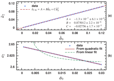
We computed the values numerically using Mathematica. Figure 5 shows the result. From the numerical data, it appears that $\tilde{a}_{2}$ is a linear function of $\tilde{\phi}_{0}$ (see Figure 5-(a)). However, a comparison of the data with the fitted linear function showed us that a higher order polynomial is better a approximations. We choose a second order polynomial since higher order polynomials do not exhibit a significant reduction of the errors. The results for $(\phi_{0},a_{2})$ variables confirm that a quadratic fit is a better approximation (see Figure 5-(b)). Note that in the interval investigated $a_{2}\sim 2.64$. In international system units, it corresponds to $10^{11}$m² (considering the typical gravitational wave sources of BBH for LIGO). This value maximizes the $f(R)$ effect for BBH collisions.

IV Evolution of equal mass binary black holes in $f(R)$ theory

IV.1 Numerical method

The evolution of the black hole and scalar field is solved using the AMSS-NCKU code (see CaoYoYu08 ; GalBruCao10a ; CaoLiu11 ; Cao12 ; CaoHil12 ). Although AMSS-NCKU code supports both vertex center and cell center grid style, we use the cell center style. We use finite difference approximation of 4th order. We update the code to include the dynamics of real scalar field equations (18) and (19). We use the outgoing radiation boundary condition for all variables. In addition, we update our code to support a combination of box and shell grid structures (according to Tho04 ; PolReiSch11 ).

The numerical grid consists of a hierarchy of nested Cartesian grid boxes and a shell which includes six coordinate patches with spherical coordinates ($\rho,\sigma,r$). For symmetric spacetimes, the corresponding symmetric patches are dropped. Particularly, we adopt equatorial symmetry. For the nested Cartesian grid boxes, a moving box mesh refinement is used. For the outer shell part, the local coordinates of the six shell patches are related to the Cartesian coordinates by

$$\pm x \text{patch:}\quad\rho=\arctan(y/x),\sigma=\arctan(z/x),$$ (48)

$$\pm y \text{patch:}\quad\rho=\arctan(x/y),\sigma=\arctan(z/y),$$ (49)

$$\pm z \text{patch:}\quad\rho=\arctan(x/z),\sigma=\arctan(y/z),$$ (50)

where both angles ($\rho,\sigma$) range over $(-\pi/4:\pi/4)$.

Notice that positive and negative Cartesian patches are related through the same coordinate transformation. This coordinate choice is right handed in $+x$, $-y$, $+z$ patches and left handed in $-x$, $+y$, $-z$ patches. Disregarding parity issues, left-handed coordinates do not bring us any inconvenience. We have applied this coordinate choice to characteristic evolutions in Cao13 . For an alternative approach, see Tho04 ; PolReiSch11 . The coordinate radius $r$ relates to the global Cartesian coordinate through

$$r=\sqrt{x^{2}+y^{2}+z^{2}}.$$ (51)

All dynamical equations for numerical evolution are written in the global Cartesian coordinate. The local coordinates ($\rho,\sigma,r$) of the six shell patches are used to define the numerical grid points with which the finite difference is implemented. The derivatives involved in the dynamical equations in the Cartesian grid $x^{i}=(x,y,z)$ are related to the spherical derivatives in the shell coordinates $r^{i}=(\rho,\sigma,r)$ through

$$\frac{\partial}{\partial x^{i}} =\left(\frac{\partial r^{j}}{\partial x^{i}}\right)\frac{\partial}{\partial r^{i}},$$ (52)

$$\frac{\partial^{2}}{\partial x^{i}\partial x^{j}} =\left(\frac{\partial r^{k}}{\partial x^{i}}\frac{\partial r^{l}}{\partial x^{j}}\right)\frac{\partial^{2}}{\partial r^{k}\partial r^{l}}+\left(\frac{\partial^{2}r^{k}}{\partial x^{i}\partial x^{j}}\right)\frac{\partial}{\partial r^{k}}.$$ (53)

The spherical derivatives in (52) and (53) are approximated by center finite difference.

In the spherical shell two patches share a common radial coordinate and adjacent patches share the angular coordinate perpendicular to the mutual boundary. Therefore, it is not necessary to perform a full 3D interpolation between the overlapping shell ghost zones. Moreover, it is enough to perform a 1D interpolation parallel to the boundary (see Tho04 ; HilBerThi12 for details). For this purpose, we use 5th order Lagrangian interpolation with the most centered possible stencil.

For the interpolation between shells and the coarsest Cartesian grid box, we use a 5th order Lagrange interpolation. This is a 3D interpolation done through three directions successively. The grid structure for boxes and shells are different. There is no parallel coordinate line between the grid structures. Therefore, we have a region which is double covered. Similar to the mesh refinement interface, we also use six buffer points in the box and shell. The buffer points are re-populated at a full Runge-Kutta time step. For parallelization, we split the shell patches into several sub-domains in three directions. The same is done for boxes.

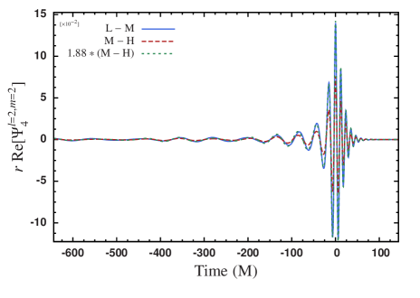
We have tested the convergence behavior of the updated AMSS-NCKU code. Fig. 6, shows the waveform produced with three resolutions. The corresponding values of the grid size for the finest refinement level are 0.009 $M$, 0.0079 $M$ and 0.007 $M$. From here-on, we refer to these values as the low (L), medium (M) and high (H) resolutions respectively. We shift the time in order to align the waveforms at the maximum amplitude of $\Psi_{4,22}$. The results presented in sections IV.2 and IV.3 are performed with the medium resolution.

Figure 6: Convergence test of the waveform. Real part of $\ell=2$, $m=2$ mode of $\Psi_{4}$. The evolution corresponds to the parameters $a_{2}=2.64418$ and $\phi_{0}=0.000959$ (see Table 3). The plot shows the differences between the low (L) and medium (M) resolutions (solid line), and the medium (M) and high (H) resolutions (dashed line). The difference between the medium and high is scaled by 1.88 which corresponds to 4th order convergence (dotted line). The corresponding values of the grid size for the finest refinement level are (L) 0.009 $M$, (M) 0.0079 $M$ and (H) 0.007 $M$.

The equation (15) represents a constraint equation which is introduced by reducing the 4th order derivative dynamical formulation to the 2nd order. Based on 3+1 formalism, we have

$${}^{(4)}R=-2\mathcal{L}_{n}K+R+K^{2}+K_{ij}K^{ij}-\frac{2}{\alpha}D_{i}D^{i}\alpha.$$ (54)

Substituting $\mathcal{L}_{n}K$ with the evolution equations for $K_{ij}$ results in

$${}^{(4)}R =8\pi(3E-S)-R-K^{2}+K_{ij}K^{ij}$$ (55)

$$=16\pi(D_{i}\phi D^{i}\phi+3V)-R-K^{2}+K_{ij}K^{ij}.$$ (56)

Therefore, the constraint equation reads as

$$\ln{\left(1+2a_{2}[16\pi(D_{i}\phi D^{i}\phi+3V)-R-K^{2}+K_{ij}K^{ij}]\right)}$$

$$=\frac{4\sqrt{\pi}}{\sqrt{3}}\phi.$$ (57)

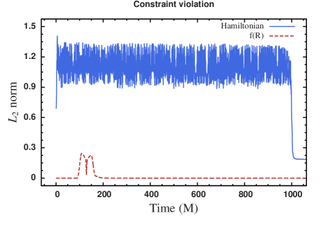
From here-on, we will refer to (57) as the $f(R)$ constraint. In Fig. 7, we show an example of the violation of this constraint during our simulations. This violation of $f(R)$ constraint is much smaller than that of the Hamiltonian constraint.

Figure 7: L2 norm of Hamiltonian constraint violation and $f(R)$ constraint violation (57). Here, $a_{2}\rightarrow\infty$ and $\phi_{0}=0.000959$.

IV.2 Initial scalar field setup

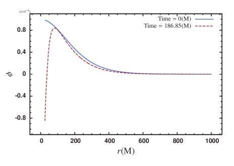
One way to interpret $f(R)$ theory is as an effective model of quantum gravity. In the astrophysical context, it is natural to assume that the systems are in their ground states, and correspondingly, the scalar field takes the profile of the ground state of the related quantum gravity system. We simulate the development of the scalar field from the ground state of the Schrödinger-Newton system considered in GuzUre04 . Other authors model the dark matter halo MagMat12 in the center of a galaxy with a similar profile (see e.g., SalBor03 ). Our result shows that the scalar field evolves from the ground state configuration to a shell-type profile (similar to (44)). Moreover, the shell forms in the early stages of the evolution. Fig. 8 shows two snapshots, the initial ground state profile and the final shell configuration. In our test, the initial profile of the scalar field is some general Gaussian shape, and the shell shape soon forms. Our results imply that the formation of a shell shape is generic in coupled systems of scalar field and BBH.

Figure 8: Snapshots of a scalar field evolving with a BBH. $\mathrm{Time}=0$ M corresponds to the ground state of the Schrödinger-Newton system considered in GuzUre04 . At $\mathrm{time}=186.85$ M, a shell shape forms.

Considering the development of a scalar field shell in the early stages of the formation of a BBH system, we starte the evolution with the profile (44). The parameters used in our simulations are listed in Table 3. We divide the parameters into three groups. The first group, $a_{2}=0$, $\phi_{0}=0$ corresponds to general relativity. The second group, $a_{2}\rightarrow\infty$ corresponds to the free EKG equations. In this case, the scalar field in the far zone is weak. Therefore, the waveforms in the Jordan frame are similar to the waveforms in the Einstein frame. The third group, $0<a_{2}<\infty$ corresponds to general $f(R)$ theory. In this case, the value $a_{2}$ is the one which maximizes $M_{\mathrm{ADM}}$ for given $\phi_{0}$.

Table 3: Parameters of the scalar field. There are three groups of parameters. $a_{2}=0$ corresponds to general relativity; $a_{2}\rightarrow\infty$ group corresponds to the EKG equations in general relativity; and $0<a_{2}<\infty$ corresponds to general $f(R)$ theory.

$M_{\mathrm{ADM}}$	$\phi_{0}$	$a_{2}$
0.99067	0	0
0.99062	0.000048	$\infty$
0.99980	0.000480	$\infty$
1.02756	0.000959	$\infty$
0.99067	0.000048	2.61877
1.00490	0.000480	2.64297
1.04790	0.000959	2.64418

IV.3 Results

In this subsection, we present the numerical simulation results for the BBH evolution in $f(R)$ theory. We focus on the comparison between $f(R)$ and GR evolution. We refer to the difference between them as the $f(R)$ effect.

IV.3.1 Dynamics of the scalar field induced by binary black holes

Figure 9: Dynamics of scalar field induced by BBH. The parameters are $a_{2}\rightarrow\infty$ and $\phi_{0}=0.000959$ (see Table 3). The upper panel (a)  shows the maximum of $|\phi|$ as a function of time. The external lower panel (b)  shows the radius position of one black hole and the corresponding radius position of the maximum of the scalar field. Internal lower panel (c)  shows the magnification of the collision part of the scalar field and the black hole.

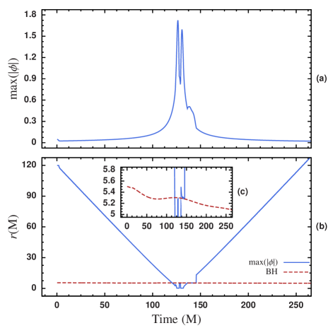
The characteristic dynamics of the scalar field in our simulations is the following. Starting from a shell shape, the scalar field collapses towards the central BBH. Then, the maximum of the scalar field reaches the black holes. At that moment in the evolution, a burst of gravitational radiation is produced . After that, the scalar field continues collapsing towards the origin of the numerical domain. The BBH excites the surrounding scalar field. The perturbations produced by the BBH collapses to the origin, thereby joining the main part of the scalar field. After reaching the origin, the scalar field is scattered in the outgoing direction. Once the scalar field moves outside of the orbit of the BBH, it is attracted by the BBH again and remains there for some time. The scalar field slowly radiates to the exterior of the numerical domain. In the process, part of the scalar field is absorbed by the black holes.

In Fig. 9-(a)  we show the maximum of $|\phi|$ with respect to time. Since the scalar field approximates a shell shape, we only consider the radial position. The change in the amplitude of the scalar field represents the collapsing stage (increments) and the scattering stage (decrements). There are two main peaks around $\mathrm{time}=125$ M. The first peak corresponds to the initial collapse (before reaching the BBH). The second peak corresponds with the excitation of the scalar field produced by the BBH. A small third peak corresponds to the attraction produced by the BBH.

Fig. 9-(b)  shows the radal position of max($|\phi|$) with respect to time (solid line) and the radial position of black hole (dashed line). The main collapsing and scattering process is clear. There are four coincidences of the scalar field and the BBH. Three of them correspond to the peaks showed in Fig. 9-(a). We enlarge the detail of the encounters in Fig. 9-(c).

As mentioned above, the collision between the scalar field and the BBH produces a burst of gravitational radiation. Fig. 10 shows the corresponding waveform of the evolution presented previously (with parameters $a_{2}\rightarrow\infty$ and $\phi_{0}=0.000959$). In this plot, we extract the waves at $r=200$ M. After the radiation produced by the initial data configuration (so-call junk radiation), there is a peak at about $\mathrm{time}=340$ M (dashed line). This burst of radiation is not present in the BBH case (solid line). Moreover, the pattern is encoded in every even $m$ mode of $\Psi_{4}$.

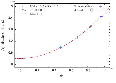
Fig. 11 shows the dependence of the amplitude of the burst as a function of $\phi_{0}$. The functional behavior is well represented by a quadratic function $A+B\phi_{0}+C\phi_{0}^{2}$, with $A=3.04\times 10^{-4}\pm 3\times 10^{-6}$, $B=-0.08\pm 0.01$ and $C=2273\pm 14$.

Figure 10: Comparison of the initial part of the waveform for a BBH collision in GR and $f(R)$ theory with parameters $a_{2}\rightarrow\infty$ and $\phi_{0}=0.000959$. The collision between the scalar field and the BBH produces a burst of gravitational radiation at roughly $\mathrm{time}=340$ M.

Figure 11: Burst amplitude as a function of the initial scalar parameter $\phi_{0}$. In this case $a_{2}\rightarrow\infty$. The fitting parameters are $A=3.04\times 10^{-4}\pm 3\times 10^{-6}$, $B=-0.08\pm 0.01$ and $C=2273\pm 14$. Notice that the value of $A$ is approximately equal to the amplitude of the waveform for GR.

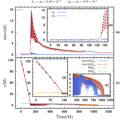
In the above description, we have presented the results for the free EKG system ($a_{2}\rightarrow\infty$). For our representative $f(R)$ case, where $a_{2}$ is finite but non-vanishing, the behavior of scalar field is qualitatively different. We compared the cases $\phi_{0}=0.000959$ and $a_{2}=2.64418$ with $\phi_{0}=0.000048$ and $a_{2}=2.61877$. Fig. 12 shows the results. Contrary to the free EKG case, we found only one collapsing stage without the scattering to infinity phase. In both cases, almost all of the scalar field was absorbed by the black holes. During the collapsing process, the scalar field excites the spacetime. The back reaction excites the scalar field, thereby producing several zig-zags in its maximum amplitude (see Figures 12-d). After the maximum of the scalar field passes over the black hole, the dynamics of scalar field become much richer. The scalar field is constantly excited near the black hole. Fig.12-(e) shows that the scalar field is trapped in the inner region of the BBH’s orbit. The black holes play the role of a semi-reflective boundary. A minor amount of scalar field escapes to infinity. In comparison with the free EKG system, the case $\phi_{0}=0.000959$ and finite $a_{2}$ introduces a large amount of eccentricity to the BBH system. However, there is no burst of gravitational radiation (which corresponds to the one presented in Fig. 10).

Figure 12: Dynamics of scalar field induced by BBH. The parameters are {$\phi_{0}=0.000048$, $a_{2}=2.61877$} (solid line) and {$\phi_{0}=0.000959$, $a_{2}=2.64418$} (dashed line). The upper panel  (a)  shows the maximum of $|\phi_{0}|$ as a function of time. The internal upper panel  (b)  shows a magnification of the initial evolution. The external lower panel  (c)  shows the radius positions of one black hole for each case (dotted and dash-dotted lines) and the corresponding radius positions of the maximum of the scalar field. Internal lower panel  (d)  shows a magnification of the collapse of the scalar field. Internal lower panel (e) shows a magnification of the merger phase. Notice that in this case the scalar field is constantly excited.

IV.3.2 Dynamics of the binary black hole induced by the scalar field

Figure 13: Coordinate separation between the black holes. Comparison between the GR vacuum case (solid line), a characteristic $f(R)$ case (dashed line) and the free EKG case (dotted line). The $f(R)$ effect makes the BBH merge faster than GR vacuum independently of the total ADM mass.

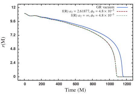
The trajectory of the BBH is strongly affected by the scalar field. When the scalar field is present, the BBH merges faster. Notice that the ADM mass is not the main cause of the fast merge. As shown in Table 3, for cases $\phi_{0}=0.00048$ and $\phi_{0}=0.000959$, the ADM mass is larger than in the GR case. On the other hand, when $\phi_{0}=0.000048$, the ADM masses for $a_{2}\rightarrow\infty$ and $a_{2}=2.61877$ are smaller and equal to the GR case respectively. However, in both cases with non-vanishing scalar field, the BBH merges faster than in the GR case (see Fig. 13).

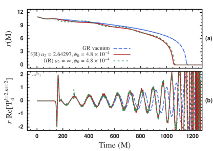
For larger values of $\phi_{0}$, for example $0.00048$, the scalar field increases the eccentricity of the BBH’s orbit in addition to making it merge faster. This extra eccentricity depends on the parameter $a_{2}$. When $a_{2}$ is big, the resulting eccentricity is large (see Fig. 14-(a)). In addition, we observe that the $f(R)$ effect makes the BBH merge faster in finite $a_{2}$ case than in the free EKG case. Previously in Sec. IV.3.1, we noticed that the interaction between the scalar field and the black hole is weaker in finite $a_{2}$ case than in the free EKG case. The behavior shown in Fig. 14-(a)  is consistent with this conclusion. When the interaction is stronger, it introduces more eccentricity to BBH evolution. More eccentric BBH orbits produce more gravitational radiation GolBru10 . Therefore, the mergers are faster.

Although the coordinate information is gauge dependent, it is possible to verify a change in the eccentricity by looking at the gravitational waves (see Fig. 14-(b)). Notice that the amplitude of the gravitational radiation burst in finite $a_{2}$ case is smaller than in the free EKG case. In Fig. 10, we can see the change in the eccentricity for the case of $\phi_{0}=0.000959$.

Figure 14: The upper panel (a)  shows the coordinate separation between the black holes. The lower panel (b)  shows the waveform ($\ell=2$, $m=2$ mode). The $f(R)$ effect introduces extra eccentricity to the BBH orbit.

So far, we have shown that small $\phi_{0}$ for free EKG cases introduces more $f(R)$ effects than finite $a_{2}$ cases. On the other hand, large $\phi_{0}$ for free EKG cases introduces less $f(R)$ effects than finite $a_{2}$ cases. It is possible that the nonlinear terms of the finite $a_{2}$ cases are the cause of these differences.

Considering the $f(R)$ effect introduced by the scalar field, we can distinguish the parameter $a_{2}$ through gravitational wave detection. LIGO’s main BBH sources are black holes with several tens of solar mass. If $a_{2}$ is bigger than $10^{11}$m², we expect to be able to distinguish between $f(R)$ theory and GR, via the gravitational detection. On the other hand, LISA (or some similar spacecraft experiment) can distinguish between $f(R)$ and GR if $a_{2}>10^{17}$m² BerGai11 . All together, the merger phase of BBH collisions allows distinction between the theories, as proposed by HeaBodHaa11 .

IV.3.3 Difference between $f(R)$ and other Einstein-Klein-Gordon models in GR

Figure 15: Trajectories and waveforms. Comparison between BBH mergers in GR, a representative case of $f(R)$ and the corresponding free EKG model. Panel (a): BBH trajectory for vacuum GR (solid line), $f(R)$ theory (dashed line) and free EKG matter model in GR (dotted line). We show the trajectory of one of the two black holes, the trajectory of the companion black hole is symmetric with respect to the $Z$ axis. The scalar field amplitude parameter is $\phi_{0}=4.8\times 10^{-4}$. Panels (b): The corresponding waveform (real part of $\Psi_{4}$, mode $\ell=2$, $m=2$). Panel (c): Same as in panel (a) but with $\phi_{0}$ ten times smaller ($\phi_{0}=4.8\times 10^{-5}$). Panel (d): Corresponding waveform for the case $\phi_{0}=4.8\times 10^{-5}$.

We have seen above that it is possible to distinguish between $f(R)$ theory and GR via the gravitational waves. Astrophysical models often include EKG equations for the description of certain phenomena. For example, there are models of dark matter which use EKG in the weak field limit AlcGuzMat02 ; BerGuz06 ; BerGuz06a ; BarBerDeg11 . One example of relativistic scalar field is boson stars Bal99 ; BalBonGuz04 ; BalComShi98 ; BalSeiSue97 ; BalBonDau06 . Therefore, it is interesting to ask if gravitational wave detection can be used to distinguish BBH collisions in $f(R)$ theory from another system which also contains scalar fields.

In the rest of this section, we analyze the differences between the free EKG system ($a_{2}\rightarrow\infty$) and the $f(R)$ theory. The main difference between free EKG and $f(R)$ theory is the nonlinear self interactions, present only in $f(R)$ theory. If the scalar field is strong, it is easy to distinguish between free EKG and $f(R)$ . If the scalar field is weak, a deeper analysis is necessary in order to distinguish between the theories. Our quantitative results support this statement.

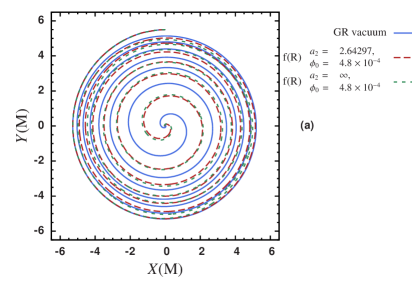
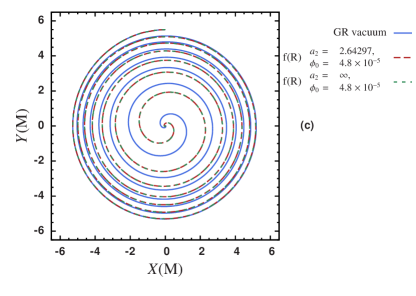
First row of Fig. 15 shows the results for $\phi_{0}=0.00048$. Fig. 15-(a)  shows the trajectory of one of the components of the binary (the companion black hole trajectory is symmetric with respect to the $X$ axis). We can see several crosses of the trajectories. This indicates different fluctuations on the inspiral rate. This results from the extra eccentricity introduced by the scalar field. In Sec. IV.3.2 and Fig. 14, we saw that the eccentricity is larger in the free EKG system than in the representative case of $f(R)$ theory. In addition, the BBH in $f(R)$ theory merges faster than in the free EKG. Therefore, it is possible to distinguish between free EKG models and $f(R)$ theory.

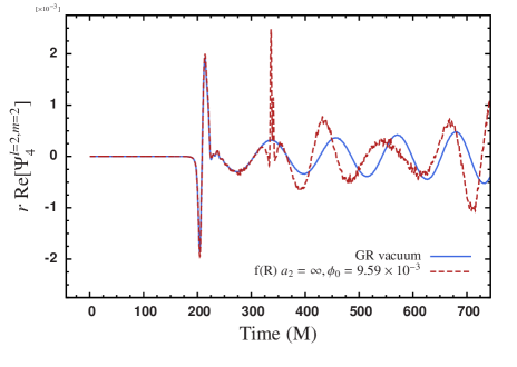
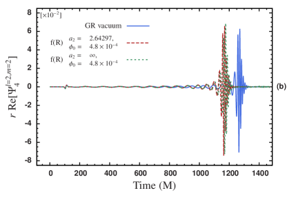
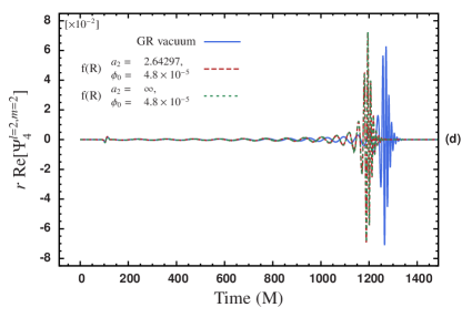
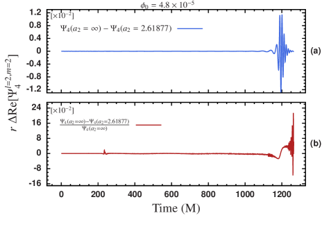
The second row of Fig. 15 shows the results for $\phi_{0}=0.000048$ (the value is ten times smaller). In this case, there are no noticeable differences between free EKG models and $f(R)$ theory. This is consistent with our assumption that the self interaction becomes weak for small scalar field. However, the quantitative difference of the $\ell=2$, $m=2$ mode of $\Psi_{4}$ is significant (see Fig. 16-(a)). Moreover, the relative difference is larger than ten percent (see Fig. 16-(b)). Once again, there is a small peak at roughly $\mathrm{time}=240$ M in Fig. 16-(b). The peak is the result of a burst of gravitational radiation produced by the free EKG model, which is absent in the $f(R)$ case (see also Fig. 10). We expect that we will be able to characterize the differences using more detailed quantitative data analysis techniques. We plan to present the results in a forthcoming paper.

Figure 16: Upper panel (a): Difference between the real part of $\Psi_{4}^{l=2,m=2}$ in $f(R)$ theory ($a_{2}=2.61877$) and free EKG model. Lower panel (b): Relative difference in amplitude of $\Psi_{4,22}$.

V Discussion

Extending the work of BerGai11 , where the extreme mass ratio BBH systems were considered to be the gravitational wave sources for LISA, we studied an equal mass BBH system. In order to simulate BBH in $f(R)$ theory with our existing numerical relativistic code, we performed transformations of the dynamical equations of $f(R)$ theory from the Jordan frame to the Einstein frame. In this way, we performed full numerical relativistic simulations. The main result in BerGai11 is that the gravitational wave detection with LISA can distinguish between $f(R)$ theory and GR if the parameter $|\mathbf{a_{2}}|>10^{17}$m². Our results imply that the gravitational wave detection with LIGO can do the same for $|\mathbf{a_{2}}|>10^{11}$m².

Mathematically, the dynamical equations of $f(R)$ theory in the Einstein frame require a scalar field. We found an interesting dynamics between this scalar field and the BBH. For example, the BBH excites the scalar field for free EKG cases ($a_{2}\rightarrow\infty$) near the collision. The scalar field is constantly excited close to the BBH for finite $a_{2}$ cases. Moreover, the interaction introduces extra eccentricity to the evolution of the BBH orbit. We found that the BBH eccentricity is affected by the initial parameter of the scalar field $\phi_{0}$ depending on the value of $a_{2}$. For small $\phi_{0}$, the excitation of the BBH orbit is larger in the representative $f(R)$ case in comparison with the free EKG system. On the other hand, for larger values of $\phi_{0}$ the excitation of the BBH orbit is smaller in the representative $f(R)$ case in comparison with the free EKG system.

Using gravitational waves, it is possible to distinguish among $f(R)$ theory, general relativity and a free Einstein-Klein-Gordon system. We found that the perturbation produced by the scalar field depends on the initial scalar field configuration. Specifically, the waveform exhibits a radiation burst which depends quadratically on the initial scalar field amplitude. The burst is a particular feature of the system which is useful when distinguishing between $f(R)$ and GR. For an initial amplitude of scalar field $\phi_{0}=0.000048$, the relative difference in the gravitational waveform between $f(R)$ theory and the free EKG model is more than 10%. Therefore, gravitational wave astronomy may provide the necessary information to rule in or rule out some alternative gravitational theories.