A Generalization of the
Directed Graph Layering Problem

Abstract

The Directed Layering Problem (DLP) solves a step of the widely used layer-based approach to automatically draw directed acyclic graphs. To cater for cyclic graphs, usually a preprocessing step is used that solves the Feedback Arc Set Problem (FASP) to make the graph acyclic before a layering is determined.

Here we present the Generalized Layering Problem (GLP), which solves the combination of DLP and FASP simultaneously, allowing general graphs as input. We present an integer programming model and a heuristic to solve the NP-complete GLP and perform thorough evaluations on different sets of graphs and with different implementations for the steps of the layer-based approach.

We observe that GLP reduces the number of dummy nodes significantly, can produce more compact drawings, and improves on graphs where DLP yields poor aspect ratios.

ayer-based layout, layer assignment, linear arrangement, feedback arc set, integer programming

Sec. 1 Introduction

The layer-based approach is a well-established and widely used method to automatically draw directed graphs. It is based on the idea to assign nodes to subsequent layers that show the inherent direction of the graph, see Fig. 1a for an example. The approach was introduced by Sugiyama et al. [19] and remains a subject of ongoing research.

Given a directed graph, the layer-based approach was originally defined for acyclic graphs as a pipeline of three phases. However, two additional phases are necessary to allow practical usage, which are marked with asterisks:

1. Cycle removal*: Eliminate all cycles by reversing a preferably small subset of the graph’s edges. This phase adds support for cyclic graphs as input.

2. Layer assignment: Assign all nodes to numbered layers such that edges point from layers of lower index to layers of higher index. Edges connecting nodes that are not on consecutive layers are split by so-called dummy nodes.

3. Crossing reduction: Find an ordering of the nodes within each layer such that the number of crossings is minimized.

4. Coordinate assignment: Determine explicit node coordinates with the goal to minimize the distance of edge endpoints.

5. Edge routing*: Compute bend points for edges, e. g. with an orthogonal style.

While state-of-the-art methods produce drawings that are often satisfying, there are graph instances where the results show bad compactness and unfavorable aspect ratio [8]. In particular, the number of layers is bound from below by the longest path of the input graph after the first phase. When placing the layers vertically one above the other, this affects the height of the drawing, see Fig. 1a. Following these observations, we present new methods to overcome current limitations.

Contributions.

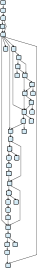
(a)

(b)

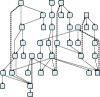
(c)

Figure 1: Different drawings of the g.39.29 graph from the North graphs collection [3]. (a) is drawn with known methods [7], (b) and (c) are results of the methods presented here. Backward edges are drawn bold and dashed.

The focus of this paper is on the first two phases stated above. They determine the initial topology of the drawing and thus directly impact the compactness and the aspect ratio of the drawing.

We introduce a new layer assignment method which is able to handle cyclic graphs and to consider compactness properties for selecting an edge reversal set. Specifically, 1) it can overcome the previously mentioned lower bound on the number of layers arising from the longest path of a graph, 2) it can be flexibly configured to either favor elongated or narrow drawings, thus improving on aspect ratio, and 3) compared to previous methods it is able to reduce both the number of dummy nodes and reversed edges for certain graphs. See Fig. 1 and Fig. 2 for examples.

We discuss how to solve the new method to optimality using an integer programming model as well as heuristically, and evaluate both.

Outline.

The next section presents related work. We introduce problems and definitions in Sec. 3, and present methods to solve the newly introduced problems in Sec. 4 and Sec. 5. Sec. 6 discusses thorough evaluations before we conclude in Sec. 7.

Sec. 2 Related Work

The cycle removal phase targets the NP-complete Feedback Arc Set Problem (FASP). Several approaches have been proposed to solve FASP either to optimality or heuristically [11]. In the context of layered graph drawing, reversing a minimal number of edges does not necessarily yield the best results, and application-inherent information might make certain edges better candidates to be reversed [7]. Moreover, the decision which edges to reverse in order to make a graph acyclic has a big impact on the results of the subsequent layering phase. Nevertheless the two phases are executed separately until today.

To solve the second phase, i. e. the layer assignment problem, several approaches with different optimization goals have emerged. Eades and Sugyiama employ a longest path layering, which requires linear time, and the resulting number of layers equals the number of nodes of the graph’s longest path [6]. Gansner et al. solve the layering phase by minimizing the sum of the edge lengths regarding the number of necessary dummy nodes [7]. They show that the problem is solvable in polynomial time and present a network simplex algorithm which in turn is not proven to be polynomial, although it runs fast in practice. This approach was found to inherently produce compact drawings and performed best in comparison to other layering approaches [10].

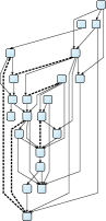
(a) 5 reversed edges, 55 dummy nodes

(b) 3 reversed edges, 34 dummy nodes

Figure 2: A graph drawn with (a) EaGa (known methods as described in Sec. 2) and (b) $1\text{-}30$-GLP (this work). This example illustrates that GLP-IP can perform better in both metrics: reversed edges (dashed) and dummy nodes.

Healy and Nikolov tackle the problem of finding a layering subject to bounds on the number of layers and the maximum number of nodes in any layer with consideration of dummy nodes using an integer linear programming approach [10]. The problem is NP-hard, even without considering dummy nodes. In a subsequent paper they present a branch-and-cut algorithm to solve the problem faster and for larger graph instances [9]. Later, Nikolov et al. propose and evaluate several heuristics to find a layering with a restricted number of nodes in each layer [14]. Nachmanson et al. present an iterative algorithm to produce drawings with an aspect ratio close to a previously specified value [13].

All of the previously mentioned layering methods have two major drawbacks. 1) They require the input graph to be acyclic upfront, and 2) they are bound to a minimum number of layers equal to the longest path of the graph. In particular this means that the bound on the number of layers in the methods of Nikolov et al. cannot be smaller than the longest path.

In the context of force-directed layout, Dwyer and Koren presented a method that can incorporate constraints enforcing all directed edges to point in the same direction [4]. They explored the possibility to relax some of the constraints, i. e. let some of the edges point backwards, and found that this improves the readability of the drawing. In particular, it reduced the number of edge crossings.

Sec. 3 Definitions and Problem Classification

Let $G=(V,E)$ denote a graph with a set of nodes $V$ and a set of edges $E$. We write an edge between nodes $u$ and $v$ as $(u,v)$ if we care about direction, as $\{u,v\}$ otherwise. A layering of a directed graph $G$ is a mapping $L:V\rightarrow\mathbb{N}$. A layering $L$ is valid if $\forall(u,v)\in E$: $L(v)-L(u)\geq 1$.

Problem (Directed Layering (DLP))

Let $G=(V,E)$ be an acyclic directed graph. The problem is to find a minimum $k$ and a valid layering $L$ such that $\sum_{(v,w)\in E}(L(w)-L(v))=k$.

As mentioned in Sec. 2, DLP was originally introduced by Gansner et al. [7]. We extend the idea of a layering for directed acyclic graphs to general graphs, i. e. graphs that are either directed or undirected and that can possibly be cyclic. Undirected graphs can be handled by assigning an arbitrary direction to each edge, thus converting it into a directed one, and by hardly penalizing reversed edges. We call a layering $L$ of a general graph $G$ feasible if $\forall\{u,v\}\in E:|L(u)-L(v)|\geq 1$.

Problem (Generalized Layering (GLP))

Let $G=(V,E)$ be a possibly cyclic directed graph and let $\omega_{\mathrm{len}},\omega_{\mathrm{rev}}\in\mathbb{N}$ be weighting constants. The problem is to find a minimum $k$ and a feasible layering $L$ such that

$$\omega_{\mathrm{len}}\left(\sum_{(v,w)\in E}\left|L(w)-L(v)\right|\right)+\omega_{\mathrm{rev}}\left|\left\{(v,w)\in E:L(v)>L(w)\right\}\right|\ =\ k\enspace.$$

Intuitively, the left part of the sum represents the overall edge length (i. e. the number of dummy nodes) and the right part represents the number of reversed edges (i. e. the FAS). After reversing all edges in this FAS, the feasible layering becomes a valid layering. Compared to the standard cycle removal phase combined with DLP, the generalized layering problem allows more flexible decisions on which edges to reverse. Also note that GLP with $\omega_{\mathrm{len}}=1,\omega_{\mathrm{rev}}=\infty$ is equivalent to DLP for acyclic input graphs and that while DLP is solvable in polynomial time, both parts of GLP are NP-complete [16].

Sec. 4 The IP Approach

In the following, we describe how to solve GLP using integer programming. The rough idea of this model is to assign integer values to the nodes of the given graph that represents the layer in which a node is to be placed.

Input and parameters. Let $G=(V,E)$ be a graph with node set $V=\{1,\dots,n\}$. Let $e$ be the adjacency matrix, i. e. $e(u,v)=1$ if $(u,v)\in E$ and $e(u,v)=0$ otherwise. $\omega_{\mathrm{len}}$ and $\omega_{\mathrm{rev}}$ are weighting constants.

Integer decision variables. $l(v)$ takes a value in $\{1,\dots,n\}$ indicating that node $v$ is placed in layer $l(v)$, for all $v\in V$.

Boolean decision variables. $r(u,v)=1$ if and only if edge $e=(u,v)\in E$ and $e$ is reversed, i. e. $l(u)>l(v)$, for all $u,v\in V$. Otherwise, $r(u,v)=0$.

$$\small\text{Minimize}\qquad\omega_{\mathrm{len}}\sum_{(u,v)\in E}|l(u)-l(v)|+\ \omega_{\mathrm{rev}}\sum_{(u,v)\in E}r(u,v)\text{.}$$

The sums represent the edge lengths, i. e. the number of dummy nodes, and the number of reversed edges, respectively. Constraints are defined as follows:

$$\small 1\ \leq\ l(v)\ \leq\ n\quad \forall v\in V$$ (A)

$$|l(u)-l(v)|\ \geq\ 1\quad \forall(u,v)\in E\quad$$ (B)

$$n\cdot r(u,v)+l(v)\ \geq\ l(u)+1\quad \forall(u,v)\in E$$ (C)

Constraint (A) restricts the range of possible layers. (B) ensures that the resulting layering is feasible. (C) binds the decision variables in $r$ to the layering, i. e. because $r$ is part of the objective, and $\omega_{\mathrm{rev}}>0$, $r(u,v)$ gets assigned 0 unless $l(v)<l(u)$, for all $(u,v)\in E$.

Variations.

The model can easily be extended to restrict the number of layers by replacing the $n$ in constraint (1) by a desired bound $b\leq n$.

The edge matrix can be extended to contain a weight $w_{u,v}$ for each edge $(u,v)\in E$. This can be helpful if further semantic information is available, i. e. about feedback edges that lend themselves well to be reversed.

Sec. 5 The Heuristic Approach

Interactive modeling tools providing automatic layout facilities require execution times significantly shorter than one second. As the IP formulation discussed in the previous section rarely meets this requirement, we present a heuristic to solve GLP. It proceeds as follows. 1) Leaf nodes are removed iteratively, since it is trivial to place them with minimum edge length and desired edge direction. Note that therefore the heuristic is not yet able to improve on trees that yield a poor compactness. We leave this for future research. 2) For the (possibly cyclic) input graph an initial feasible layering is constructed which is used to deduce edge directions yielding an acyclic graph. 3) Using the network simplex method presented by Gansner et al. [7], a solution with minimal edge length is created. 4) We execute a greedy improvement procedure after which we again deduce edge directions and re-attach the leaves. 5) We apply the network simplex algorithm a second time to get a valid layering with minimal edge lengths for the next steps of the layer-based approach. In the following we will discuss steps 2 and 4 in further detail.

Step 2: Layering Construction.

To construct an initial feasible solution we follow an idea that was first presented by McAllister as part of a greedy heuristic for the Linear Arrangement Problem (LAP) [12] and later extended by Pantrigo et al. [15].

Nodes are assigned to distinct indexes, where as a start, a node is selected randomly, assigned to the first index, and added to a set of assigned nodes. Based on the set of assigned nodes a candidate list is formed, and the most promising node is assigned to the next index. As decision criterion we use the difference between the number of edges incident to unassigned nodes and the number of edges incident to assigned nodes. This procedure is repeated until all nodes are assigned to distinct indices (see Alg. 1).

In contrast to McAllister, for GLP we allow nodes to be added to either side of the set of assigned nodes, and decide the side based on the number of reversed edges that would emerge from placing a certain node on that side. For this we use a decreasing left index variable and an increasing right index variable.

Input: directed graph $G=(V,E)$

Data: Sets $U$, $C$. For all $v\in V$ $score[v],incAs[v],outAs[v]$

$lIndex\leftarrow-1$, $rIndex\leftarrow 0$

Output: index[v]: feasible layering of G

1 for $v\in V$ do

2       $score[v]\leftarrow|\{w\enspace|\enspace\{v,w\}\in E\}|$; $incAs[v]\leftarrow 0$; $outAs[v]\leftarrow 0$

3       add $v$ to $U$

4remove random $v$ from $U$

5 $c\leftarrow v$

6 while $U$ not empty do

7       if $incAs[c]<outAs[c]$ then

8             $index[c]\leftarrow lIndex$$-$ $-$

9      else

10             $index[c]\leftarrow rIndex$$+$$+$

11      remove $c$ from $U$ and $C$; $cScore\leftarrow\infty$

12       for $v\in\{w\enspace|\enspace\{c,w\}\in E\wedge w\in U\}$ do

13             add $v$ to $C$; $score[v]$$-$ $-$

14             if $(c,v)\in E$ then $incAs[v]$$+$$+$ else $outAs[v]$$+$$+$

15             

16      for $v\in C$ do

17             if  $score[v]<cScore$  then  $cScore\leftarrow score[v]$; $c\leftarrow v$

18            

19      

Algorithm 1 constructLayering

Step 4: Layering Improvement.

At this point a feasible layering with a minimum number of dummy nodes w. r. t. the chosen FAS is given since we execute the network simplex method of Gansner et al. beforehand. Thus we can only improve on the number of reversed edges. We determine possible moves and decide whether to take the move based on a profit value. Let a graph $G=(V,E)$ and a feasible layering $L$ be given. For ease of presentation, we define the following notions. An example: For a node $v$, topSuc are the nodes connected to $v$ via an outgoing edge of $v$ and are currently assigned to a layer with lower index than $v$’s index. Intuitively, topSuc (just as botPre) are nodes connected by an edge pointing into the “wrong” direction.

$$v.\textit{\scriptsize topSuc}=\{w:(v,w)\in E\wedge L(v)>L(w)\} v.\textit{\scriptsize botSuc}=\{w:(v,w)\in E\wedge L(v)<L(w)\}$$

$$v.\textit{\scriptsize topPre}=\{w:(w,v)\in E\wedge L(w)<L(v)\} v.\textit{\scriptsize botPre}=\{w:(w,v)\in E\wedge L(w)>L(v)\}$$

$$v.\textit{\scriptsize topAdj}=v.\textit{\scriptsize topSuc}\cup v.\textit{\scriptsize topPre} v.\textit{\scriptsize botAdj}=v.\textit{\scriptsize botSuc}\cup v.\textit{\scriptsize botPre}$$

For all these functions we define suffixes that allow to query for a certain set of nodes before or after a certain index. For instance, for all top successors of $v$ before index $i$ we write $v.\textit{\scriptsize topSucBefore(i)}=\{w:w\in v.\textit{\scriptsize topSuc}\wedge L(w)<i\}$.

Let $move:V\mapsto\mathbb{N}$ denote a function assigning to each node a natural value. The function describes whether it is possible to move a node without violating the layering’s feasibility as well as how far the node should be moved. For instance, let for a node $v$ topPre be empty but topSuc be not empty. Thus, we can move $v$ to an arbitrary layer with lower index than $L(v)$. A good choice would be one layer before any of $v$’s topSuc since this would alter the connected edges to point downwards.

$$move(v)=\left\{\begin{array}[]{l l}0&\quad\text{if }v.\textit{\scriptsize topSuc}=\emptyset,\\ L(v)-\min(\{L(w):w\in v.\textit{\scriptsize topSuc}\})+1&\quad\text{if }v.\textit{\scriptsize topPre}=\emptyset,\\ L(v)-\max(\{L(w):w\in v.\textit{\scriptsize topPre}\})-1&\quad\text{otherwise.}\end{array}\right.$$

Let $\mbox{profit}:V\times\mathbb{N}\times\mathbb{N}\mapsto\mathbb{Z}$ denote a function assigning a quality score to each node $v$ if it were moved by $m\in\mathbb{N}$ to a different layer $x$, i. e. if it is worth to increase some edges’ lengths for a subset of them to point downwards. Note that we reuse $\omega_{\mathrm{len}}$ and $\omega_{\mathrm{rev}}$ here but do not expect them to have an impact as strong as for the IP. For the rest of the paper we fix them to 1 and 5.

$$\mbox{profit}(v,m,x)=\left\{\begin{array}[]{l l}0&\quad\text{if }m\leq 1,\\ \omega_{\mathrm{len}}(m|v.\textit{\scriptsize topAdjBefore(x)}|-m|v.\textit{\scriptsize botAdj}|)&\\ +\enspace\omega_{\mathrm{rev}}|v.\textit{\scriptsize topSucAfter(x)}|&\quad\text{otherwise.}\end{array}\right.$$

As seen in Alg. 2, the $move$ and profit functions are determined initially for a given feasible layering. A queue, sorted based on profit values, is then used to successively perform moves that yield a profit. After a move of node $n$, both functions can be updated for all nodes in the adjacency of $n$.

Input: feasible layering of $G=(V,E)$ in $index[v]$

Data: priority queue PQ

For all $v\in V$ $move[v]$, $\mbox{{profit}}[v]$

Output: index[v]: feasible layering of G

1 for $v\in V$ do

2       $move[v]\leftarrow move(v)$

3       $\mbox{{profit}}[v]\leftarrow\mbox{{profit}}(v,\ move[v],\ index[v]-move[v])$

4       if  $\mbox{{profit}}[v]>0$  then  enqueue $v$ to $PQ$

5      

6while $PQ$ not empty do

7       $v\leftarrow$ dequeue $PQ$

8       $index[v]$ $-$ $=$$\enspace move[v]$

9       for $w\in\{w\enspace|\enspace\{v,w\}\in E\}$ do

10             update $move[w]$ and $\mbox{{profit}}[w]$

11             if  $\mbox{{profit}}[w]>0$  then enqueue $w$ to $PQ$ else  possibly dequeue $w$ from $PQ$

12             

13      

Algorithm 2 improveLayering

Time Complexity.

Removing leaf nodes requires linear time, $O(|V|+|E|)$. Alg. 1 is quadratic in the number of nodes, $O(|V|^{2})$. The while loop has to assign an index to every node and the two inner for loops are, for a complete graph, iterated $\frac{|V|}{2}$ times on average. Determining the next candidate (lines 15–16) could be accelerated using dedicated data structures. The improvement step strongly depends on the input graph. The network simplex method runs reportedly fast in practice [7], although it has not been proven to be polynomial. Our evaluations showed that the heuristic’s overall execution time is clearly dominated by the network simplex method (cf. Sec. 6).

Sec. 6 Evaluation

In this section we evaluate three points: 1) the general feasibility of GLP to improve the compactness of drawings, 2) the quality of metric estimations for area and aspect ratio, and 3) the performance of the presented IP and heuristic. Our main metrics of interest here are height, area, and aspect ratio, as defined in an earlier paper [8]. Remember that the layer-based approach is defined as a pipeline of several independent steps. After the layering phase, which is the focus of our research here, these latter two metrics can only be estimated using the number of dummy nodes, the number of layers, and the maximal number of nodes in a layer. Results can be seen in Tab. 1 and Tab. 2, which we will discuss in more detail in the remainder of this section.

Obtaining a Final Drawing.

To collect all metrics we desire, we have to create a final drawing of a graph. Over time numerous strategies have been presented for each step of the layer-based approach, we thus present several alternatives. To break cycles we use a popular heuristic by Eades et al. [5]. To determine a layering we use our newly presented approach GLP (both the IP method and heuristic, denoted by GLP-IP and GLP-H) and alternatively the network simplex method presented by Gansner et al. [7]. We denote the combination of the cycle breaking of Eades et al. and the layering of Gansner et al. as EaGa and consider it to be an alternative to GLP. Crossings between pairs of layers are minimized using a layer sweep method in conjunction with the barycenter heuristic, as originally proposed by Sugiyama et al. [19]. We employ two different strategies to determine fixed coordinates for nodes within the layers. First, we consider a method introduced by Buchheim et al. that was extended by Brandes and Köpf [2, 1], which we denote as BK. Second, we use a method inspired by Sander [17] that we call LS. Edges are routed either using polylines (Poly) or orthogonal segments (Orth). The orthogonal router is based on the methods presented by Sander [18]. Overall, this gives twelve setups of the algorithm: three layering methods, two node placement algorithms, and two edge routing procedures. In the following, let $\omega_{\mathrm{len}}$-$\omega_{\mathrm{rev}}$-GLP denote the used weights. If we do not further qualify GLP, we refer to the IP model.

Table 1: Average values for different layering strategies employed to the test graphs. Different weights are used for GLP-IP as specified in the column head and final drawings were created using BK and Poly. For $\text{\acs{glph}}^{*}$ no improvement was performed. A detailed version of these results is included in the appendix (cf. 0.A.2).

	1-10	1-20	1-30	1-40	1-50	EaGa	GLP-H	$\text{\acs{glph}}^{*}$
Reversed edges	3.71	2.89	2.64	2.54	2.44	2.93	8.67	10.36
Dummy nodes	34.45	46.73	52.79	56.14	60.53	72.64	48.48	58.21
Height	843	943	980	1,004	1,025	1,084	930	1,027
Area	631,737	672,717	691,216	700,385	708,361	737,159	656,070	720,798
Aspect ratio	0.77	0.65	0.63	0.61	0.59	0.55	0.67	0.60

(a) Random graphs

	1-10	1-20	1-30	1-40	1-50	EaGa	GLP-H	$\text{GLP-H}^{*}$
Reversed edges	2.74	1.47	1.02	0.72	0.56	0	7.07	8.55
Dummy nodes	39.91	55.47	65.73	75.66	82.47	141.30	53.53	68.91
Height	1,068	1,224	1,334	1,409	1,469	1,727	1,137	1,216
Area	587,727	622,838	641,581	660,842	695,494	874,374	629,778	691,372
Aspect ratio	0.34	0.28	0.24	0.23	0.22	0.20	0.33	0.32

(b) North graphs

Test Graphs.

Our new approach is intended to improve the drawings of graphs with a large height and relatively small width, hence unfavorable aspect ratio. Nevertheless, we also evaluate the generality of the approach using a set of 160 randomly generated graphs with 17 to 60 nodes and an average of $1.5$ edges per node. The graphs were generated by creating a number of nodes, assigning out-degrees to each node such that the sum of outgoing edges is $1.5$ times the nodes, and finally creating the outgoing edges with a randomly chosen target node. Unconnected nodes were removed. Second, we filtered the graph set provided by North [3] based on the aspect ratio and selected 146 graphs that have at least 20 nodes and a drawing with an aspect ratio below $0.5$, i. e. are at least twice as high as wide. We also removed plain paths, that is, pairs of nodes connected by exactly one edge, and trees. For these special cases GLP in its current form would not change the resulting number of reversed edges as all edges can be drawn with length $1$. This is also true for any bipartite graph. Note however that GLP can easily incorporate a bound on the number of layers which can straightforwardly be used to force more edges to be reversed, resulting in a drawing with better aspect ratio.

General Feasibility of GLP.

An exemplary result of the GLP approach compared to EaGa can be seen in Fig. 2. For that specific drawing, GLP produces fewer reversed edges, fewer dummy nodes, and less area (both in width and height). For all tested setups the average effective height and area (normalized by the number of nodes) of GLP and the heuristic are smaller than EaGa’s, see Tab. 2. The average aspect ratios come closer to $1.0$. For simplicity, in this paper we desire aspect ratios closer to $1.0$. For a more detailed discussion on this topic see Gutwenger et al. [8].

Furthermore, we found that by altering the weights $\omega_{\mathrm{rev}}$ and $\omega_{\mathrm{len}}$ a trade-off between reversed edges and resulting dummy nodes (and thus area and aspect ratio) can be achieved, which can be seen in Tab.1a.

The results for the North graphs are similar. Since the North graphs are acyclic, the cycle breaking phase is not required and current layering algorithms cannot improve the height. The GLP approach, however, can freely reverse edges and hereby change the height and aspect ratio. Results can be seen in Tab. 1b. Clearly, EaGa has no reversed edges as all graphs are acyclic. $1\text{-}10$-GLP starts with an average of $2.7$ reversed edges and the value constantly decreases with an increased weight on reversed edges. The number of dummy nodes on the other hand constantly decreases from $141.3$ for EaGa to $39.9$ for $1\text{-}10$-GLP.

The average height and average area of the final drawings decrease with an increasing number of reversed edges. For $1\text{-}10$-GLP the average height and area are 38.2 % and 33.8 % smaller than EaGa. The aspect ratio changes from an average of 0.20 for EaGa to 0.34 for $1\text{-}10$-GLP.

The results show that for the selected graphs, for which current methods cannot improve on height, the weights of the new approach allow to find a satisfying trade-off between reversed edges and dummy nodes. Furthermore, the improvements in compactness stem solely from the selection of weights, not from an upper bound on the number of layers. Naturally, such a bound can further improve the aspect ratio and height.

Table 2: Results for final drawings of the set of random graphs, when applying different layout strategies. For GLP-IP $\omega_{\mathrm{len}}=1$ and $\omega_{\mathrm{rev}}=30$ were used. Area is normalized by a graph’s node count. The most interesting comparisons are between columns where EaGa and GLP use the same strategies for the remaining steps. Detailed results can be found in the appendix (cf. 0.A.2).

Edge routing	Poly						Orth
Node coord.	BK			LS			BK			LS
Layering	EaGa	GLP-IP	GLP-H	EaGa	GLP-IP	GLP-H	EaGa	GLP-IP	GLP-H	EaGa	GLP-IP	GLP-H
Height	1,165	1,043	898	943	824	732	790	711	652	817	746	678
Area	20,194	18,683	15,575	12,383	11,035	10,075	13,582	12,642	11,272	10,666	9,917	9,295
Aspect ratio	0.59	0.67	0.67	0.55	0.64	0.64	0.84	0.96	0.90	0.63	0.70	0.68

Metric Estimations.

Tab. 2 presents results that were measured on the final drawing of a graph. As mentioned earlier, after the layering step these values are not available and estimations are commonly used to deduce the quality of a result. For our example graphs, the estimated area reduced from $222.9$ (EaGa) to $187.4$ ($1\text{-}30$-GLP) on average. The estimated aspect ratios increase on average from $0.74$ to $0.84$. Both tendencies conform to the averaged effective values in Tab. 2, i. e. GLP-IP and the GLP-H perform better. However, we observed that for 64 % of the graphs the tendency of the estimated area contradicts the tendency of the effective area. 54 % when not considering dummy nodes. In other words, for a specific graph the estimated area might be decreased for GLP compared to EaGa but the effective area is increased for GLP (or vice versa). This clearly indicates that an estimation can be misleading. Besides, node placement and edge routing can have a non-negligible impact on the aspect ratio and compactness of the final drawing.

Performance of the Heuristic.

Results for final drawings using the presented heuristic are included in Tab. 2 and are comparable to $1\text{-}30$-GLP, i. e. the heuristic performs better than EaGa  w. r. t. the desired metrics.

Tab. 1a and Tab. 1b underline this result and show that the improvement step of the heuristic clearly improves on all measured metrics. Further, more detailed results, can be found in the appendix. Nevertheless, the heuristic yields significantly more reversed edges. When aiming for compactness, we consider this to be acceptable.

Execution Times.

To solve the IP model we used CPLEX 12.6 and executed the evaluations on a server with an Intel Xeon E5540 CPU and 24 GB memory. The execution times for GLP-IP vary between 476ms for a graph with 19 nodes and 541s for a graph with 58 nodes and exponentially increase with the graph’s node count. This is impracticable for interactive tools that rely on automatic layout, but is fast enough to collect optimal results for medium sized graphs.

The execution time of the heuristic is compared to EaGa and was measured on a laptop with an Intel i7-3537U CPU and 8 GB memory. The reported time includes only the first two steps of the layer-based approach. It turns out that the execution time of the heuristic is on average 2.3 times longer than EaGa. This seems reasonable, as it involves two executions of the network simplex layering method. For the tested graphs, the construction and improvement steps of the heuristic hardly contribute to its overall execution time. The effective execution time ranges between 0.1ms and 10.0ms for EaGa and 0.3ms and 19.7ms for the heuristic. Hence, the heuristic is fast enough to be used in interactive tools.

We also ran the algorithm five times for five randomly generated graphs with 1000 nodes and 1500 edges. EaGa required an average of 374ms, the heuristic 666ms with about 4ms for construction an 2ms for improvement. This shows that the time contribution of the latter two is negligible even for larger graphs.

Sec. 7 Conclusion

In this paper we address problems with current methods for the first two phases of the layer-based layout approach. We argue that separately performing cycle breaking and layering is disadvantageous when aiming for compactness.

We present a configurable method for the layering phase that, compared to other state-of-the-art methods, shows on average improved performance on compactness. That is, the number of dummy nodes is reduced significantly for most graphs and can never increase. While the number of dummy nodes only allows for an estimation of the area, the effective area of the final drawing is reduced as well. Furthermore, graph instances for which current methods yield unfavorable aspect ratios can easily be improved. Also, the presented heuristic clearly improves on the desired metrics. Depending on the application, a slight increase in the number of reversed edges is often acceptable.

We want to stress that the common practice to determine the quality of methods developed for certain phases of the layer-based approach based on metrics that represent estimations of the properties of the final drawing is error-prone. For instance, estimations of the area and aspect ratio after the layering phase can vary significantly from the effective values of the final drawing and strongly depend on the used strategies for computing node and edge coordinates.

Future work will include improving the heuristic, e. g. selecting the initial node based on a certain criterion instead of randomly in Alg. 1 should improve the results. We also plan to incorporate hard bounds on the width of a drawing. It is important that methods support to prevent, or at least to strongly penalize, the reversal of certain edges, since certain diagram types demand several edges to be drawn forwards. Also, user studies could help understand which edges are natural candidates to be reversed from a human’s perspective.

Furthermore, in an accompanying technical report we present a variation of GLP where we fix the size of the FAS while remaining free in the choice of which edges to reverse [16], which so far has only been evaluated using integer programming.

7.0.1 Acknowledgements.

We thank Chris Mears for support regarding the initial IP formulation. We further thank Tim Dwyer and Petra Mutzel for valuable discussions. This work was supported by the German Research Foundation under the project Compact Graph Drawing with Port Constraints
(ComDraPor, DFG HA 4407/8-1).

Appendix 0.A Appendix

0.A.1 Example Drawings of North Graphs

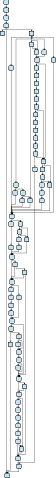
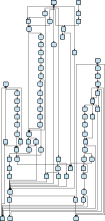
(a) g.75.1

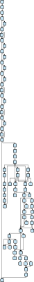
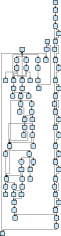
(b) g.80.5

Figure 3: For each graph the left drawing is produced using EaGa and the right drawing using the GLP-H as presented here. Graphs are taken from the North graphs library.

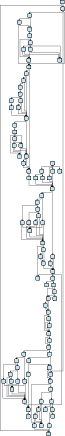
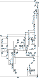
(a) g.99.0

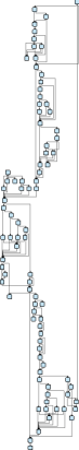
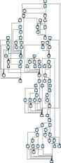
(b) g.86.5

Figure 4: For each graph the left drawing is produced using EaGa and the right drawing using the GLP-H heuristic as presented here. Graphs are taken from the North graphs library.

0.A.2 Detailed Results

Figure 5: Random graphs: Detailed results in the form of boxplots. A summary can be seen in Tab.1a. The dashed line represents the median of EaGa. Lower values are better, with the exception of the aspect ratio. It can be seen that the methods presented here, improve the drawing w. r. t. the relevant metrics. It is noteworthy that for $1\text{-}30$-GLP, $1\text{-}40$-GLP, and $1\text{-}50$-GLP, both the number of reversed edges and the number of dummy nodes is smaller compared to EaGa.

Figure 6: North graphs: Detailed results in the form of boxplots. A summary can be seen in Tab.1b. The dashed line represents the median of EaGa. Lower values are better, with the exception of the aspect ratio. It can be seen that the methods presented here, improve the drawing w. r. t. the relevant metrics. The North graphs are acyclic which is why EaGa consistently produces zero reversed edges. The aspect ratio of the majority of the graphs improves significantly with a constant to slightly improved area.

Figure 7: Detailed results for the produced drawings using different strategies for the layer-based approach’s phases as discussed in Sec. 6 (cf. Tab. 2). It can be seen that for every combination GLP-IP and GLP-H improve w. r. t. the tested metrics when compared to EaGa. Furthermore, the results emphasize that different strategies can result in significantly different drawings, especially when it comes to aspect ratio. For instance, orthogonal-style edges allow for less height and area. Node coordinates assigned by LS tend to allow for smaller area than BK.

References

- [1] U. Brandes and B. Köpf. Fast and simple horizontal coordinate assignment. In Proceedings of the 9th International Symposium on Graph Drawing (GD’01), volume 2265 of LNCS, pages 33–36. Springer, 2002.
- [2] C. Buchheim, M. Jünger, and S. Leipert. A fast layout algorithm for -level graphs. In J. Marks, editor, Proceedings of the 8th International Symposium on Graph Drawing (GD’00), volume 1984 of LNCS, pages 229–240. Springer, 2001.
- [3] G. Di Battista, A. Garg, G. Liotta, A. Parise, R. Tamassia, E. Tassinari, F. Vargiu, and L. Vismara. Drawing directed acyclic graphs: An experimental study. In Proceedings of the Symposium on Graph Drawing (GD’96), volume 1190 of LNCS, pages 76–91. Springer, 1997.
- [4] T. Dwyer and Y. Koren. Dig-CoLa: directed graph layout through constrained energy minimization. In Proceedings of the IEEE Symposium on Information Visualization (INFOVIS’05), pages 65–72, Oct. 2005.
- [5] P. Eades, X. Lin, and W. F. Smyth. A fast and effective heuristic for the feedback arc set problem. Information Processing Letters, 47(6):319–323, 1993.
- [6] P. Eades and K. Sugiyama. How to draw a directed graph. Journal of Information Processing, 13(4):424–437, 1990.
- [7] E. R. Gansner, E. Koutsofios, S. C. North, and K.-P. Vo. A technique for drawing directed graphs. Software Engineering, 19(3):214–230, 1993.
- [8] C. Gutwenger, R. von Hanxleden, P. Mutzel, U. Rüegg, and M. Spönemann. Examining the compactness of automatic layout algorithms for practical diagrams. In Proceedings of the Workshop on Graph Visualization in Practice (GraphViP’14), Melbourne, Australia, July 2014.
- [9] P. Healy and N. S. Nikolov. A branch-and-cut approach to the directed acyclic graph layering problem. In Proceedings of the 10th International Symposium on Graph Drawing (GD’02), volume 2528 of LNCS, pages 98–109. Springer, 2002.
- [10] P. Healy and N. S. Nikolov. How to layer a directed acyclic graph. In Proceedings of the 9th International Symposium on Graph Drawing (GD’01), volume 2265 of LNCS, pages 563–566. Springer, 2002.
- [11] P. Healy and N. S. Nikolov. Hierarchical drawing algorithms. In R. Tamassia, editor, Handbook of Graph Drawing and Visualization, pages 409–453. CRC Press, 2013.
- [12] A. J. McAllister. A new heuristic algorithm for the linear arrangement problem. Technical report, University of New Brunswick, 1999.
- [13] L. Nachmanson, G. Robertson, and B. Lee. Drawing graphs with GLEE. In S.-H. Hong, T. Nishizeki, and W. Quan, editors, Graph Drawing, volume 4875 of LNCS, pages 389–394. Springer Berlin Heidelberg, 2008.
- [14] N. S. Nikolov, A. Tarassov, and J. Branke. In search for efficient heuristics for minimum-width graph layering with consideration of dummy nodes. Journal of Experimental Algorithmics, 10, 2005.
- [15] J. Pantrigo, R. Martí, A. Duarte, and E. Pardo. Scatter search for the cutwidth minimization problem. Annals of Operations Research, 199(1):285–304, 2012.
- [16] U. Rüegg, T. Ehlers, M. Spönemann, and R. von Hanxleden. A generalization of the directed graph layering problem. Technical Report 1501, Christian-Albrechts-Universität zu Kiel, Department of Computer Science, Feb. 2015. ISSN 2192-6247.
- [17] G. Sander. A fast heuristic for hierarchical Manhattan layout. In F. J. Brandenburg, editor, Proceedings of the Symposium on Graph Drawing (GD’95), volume 1027 of LNCS, pages 447–458. Springer, 1996.
- [18] G. Sander. Layout of directed hypergraphs with orthogonal hyperedges. In Proceedings of the 11th International Symposium on Graph Drawing (GD’03), volume 2912 of LNCS, pages 381–386. Springer, 2004.
- [19] K. Sugiyama, S. Tagawa, and M. Toda. Methods for visual understanding of hierarchical system structures. IEEE Transactions on Systems, Man and Cybernetics, 11(2):109–125, Feb. 1981.