Photospheric Magnetic Free Energy Density of Solar Active Regions
Solar Physics

1 Introduction

The relationship of non-potential magnetic fields in active regions to solar flares and coronal mass ejections (CMEs) is an interesting topic of study. It is believed that the non-potential magnetic fields are generated inside the Sun and then transported from the sub-atmosphere into interplanetary space. The photospheric non-potential magnetic field formed in active regions is also important for triggering the powerful solar flares and CMEs (cf. Schmieder et al., 1994) because it is difficult to accurately estimate the topology of the magnetic lines of force in the high solar atmosphere without any information about the photospheric magnetic fields. Moreover, the associated change in photospheric vector magnetic fields with powerful flares in active regions has been detected from observations made with magnetographs (cf. Chen et al., 1989). This means that the analysis of photospheric magnetic fields is very important for understanding solar eruptions.

The magnetic shear inferred from observational photospheric vector magnetograms is an important parameter to provide information about the magnetic non-potentiality in solar active regions (cf. Krall et al., 1982; Lü, Wang and Wang, 1993), while the vertical electric current and current helicity inferred from vector magnetograms mainly provide information about the spatial non-uniformity and chirality of magnetic fields in the photosphere (cf. Severny, 1971; Hagyard, Low and Tandberg-Hanssen, 1981; Seehafer, 1994; Zhang, 1995). The magnetic fields and their free energy above the photosphere can be inferred by photospheric vector magnetograms in the approximation of force-free magnetic fields (Chandrasekhar, 1961; Low, 1982). Many questions remain, however, about the analysis of the real configuration of magnetic fields in the solar atmosphere because it is difficult to use spectral information to accurately measure the vector magnetic field above the photosphere. In this situation, obtaining more information from the observational photospheric vector magnetic fields and corresponding parameters becomes very important.

In this articale, we analyze the energy distribution of magnetic fields in the photosphere inferred from the observational vector magnetograms in flare-producing active regions.

2 Definition of Free Magnetic Energy Density

S-fed The energy released by solar flares and other explosive events relies on the accumulation of the free magnetic energy (non-potential magnetic energy), which is defined as the difference between the total magnetic energy ($E_{o}$) and the potential magnetic energy ($E_{p}$):

eq:MGshenergy$$\Delta E=E_{o}-E_{p}.$$ (1)

This means that the free energy is defined with respect to the energy of the potential field that matches the distribution of the observed field’s normal component. This potential field has the lowest possible magnetic energy that is still consistent with the boundary condition (for example see Priest, 2014).

The total magnetic energy of a field $\bf B$ is given in the form

$$\ilabel{eq:int}E=\int B^{2}dV,$$ (2)

which means that the magnetic energy is a three-dimensional integral quantity, such as in the solar atmosphere.

Hagyard, Low and Tandberg-Hanssen (1981) defined the source field to describe the non-potentiality of magnetic field on the photosphere:

eq:MGshear$$\emph{{B}}_{n}=\emph{{B}}_{o}-\emph{{B}}_{p},$$ (3)

where $\emph{{B}}_{o}$ is the observed vector magnetic field, $\emph{{B}}_{p}$ denotes the potential field extrapolated from the vertical component of $\emph{{B}}_{o}$, and $\emph{{B}}_{n}$ is the so-called source field, that is, the non-potential component of the magnetic field. By means of Equation (eq:MGshear), it is found

$$\ilabel{}B_{n}=\sqrt[]{B_{o}^{2}+B_{p}^{2}-2B_{o}B_{p}\cos\psi},$$ (4)

where $\psi$ is the inclined angle between ${\bf B}_{o}$ and ${\bf B}_{p}$ in Figure fig:MGsh0.

Now we can introduce the magnetic energy density $\rho$, as in $\displaystyle E=\int\frac{B^{2}}{8\pi}dV=\int\rho dV$, where the field energy density $\rho\equiv B^{2}/8\pi$. Analogously, for $E_{o}$ and $E_{p}$, the observed and potential-field energy density are $\rho_{o}\equiv B_{o}^{2}/8\pi$ and $\rho_{p}\equiv B_{p}^{2}/8\pi$, respectively. We also note that the free energy density integrated over a volume $V$ yields an energy, and the free energy density integrated over the photosphere yields a quantity with dimensions of energy per unit length. This quantity is not, strictly speaking, a free energy, but it is plausibly related to the free energy present in the volume above the photosphere. The observation of photospheric vector magnetograms provides an opportunity to analyze the distribution of magnetic energy density in the low solar atmosphere. We exclusively consider two-dimensional arrays of magnetic energy from photospheric magnetic fields in the following.

The energy density parameter of the non-potential magnetic field as defined by Lü, Wang and Wang (1993) is proportional to $\emph{{B}}_{n}^{2}$:

$$\rho_{n}=\frac{(\emph{{B}}_{o}-\emph{{B}}_{p})^{2}}{8\pi}=\frac{\emph{{B}}_{n}^{2}}{8\pi}.$$ (5)

This energy parameter had been also used to analyze the solar magnetic active cycles (Yang et al., 2012).

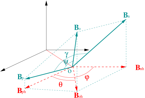
Figure 1.: A schematic of the relationships among the observed magnetic field ${\bf B}_{o}$, the potential field ${\bf B}_{p}$, and the non-potential field ${\bf B}_{n}$. The arrows in red indicate their respective horizontal components. fig:MGsh0

It follows that the definition of the real free energy density (Equation (eq:MGshenergy)) is

$$\rho_{free}=\rho_{o}-\rho_{p}=\frac{{\bf B}_{o}^{2}-{\bf B}_{p}^{2}}{8\pi}=\frac{({\bf B}_{n}+{\bf B}_{p})^{2}-{\bf B}_{p}^{2}}{8\pi},$$ (6)

and it can be written

$$\rho_{free} = \frac{1}{8\pi}{B}_{n}^{2}+\frac{1}{4\pi}{\bf B}_{n}\cdot{\bf B}_{p}=\frac{1}{8\pi}{B}_{n}^{2}+\frac{1}{4\pi}{B}_{n}{B}_{p}\cos\gamma$$ (7)

$$= \frac{1}{8\pi}{B}_{n}^{2}+\frac{1}{4\pi}B_{n}B_{p}\cos\left[\psi+\cos^{-1}\left(\frac{B_{o}-B_{p}\cos\psi}{B_{n}}\right)\right],$$

where $\gamma$ and $\psi$ are spatial angles, and $\cos^{-1}\left(\frac{B_{o}-B_{p}\cos\psi}{B_{n}}\right)=\gamma-\psi$, in Figure fig:MGsh0. We can find the relationship

$$\cos\left[\psi+\cos^{-1}\left(\frac{B_{o}-B_{p}\cos\psi}{B_{n}}\right)\right]$$

$$=\sin\vartheta_{p}\sin\vartheta_{n}+\cos\vartheta_{p}\cos\vartheta_{n}\cos\left[\theta+\cos^{-1}\left(\frac{B_{oh}-B_{ph}\cos\theta}{B_{nh}}\right)\right],$$ (8)

where $\vartheta_{n}$ is the inclination angle between the vector of the non-potential field ${\bf B}_{n}$ and its horizontal component ${\bf B}_{nh}$, and $\vartheta_{p}$ is that between the vector of the potential field ${\bf B}_{p}$ and its horizontal component ${\bf B}_{ph}$, while the angle $\theta$ is defined as the horizontal angle between ${\bf B}_{oh}$ and ${\bf B}_{ph}$, and $\cos^{-1}\left(\frac{B_{oh}-B_{ph}\cos\theta}{B_{nh}}\right)=\varphi-\theta$, in Figure fig:MGsh0.

Because we cannot directly measure the vertical component of the non-potential magnetic field in the photospheric layer from the observational vector magnetograms, we normally require a model field to match the observed vertical field, whether in the analysis of non-potential fields or potential fields. For potential models, this choice corresponds to the Neumann boundary condition (see, for instance, Sakurai, 1982), although observations of changes in vertical magnetic fields associated with flares demonstrate that the observed vertical field is not generally consistent with the lowest energy state of the field. This means that the vertical component of the magnetic field does not contribute to the magnetic free energy density from the photospheric vector magnetograms. For observations near disk center, we can approximate the line-of-sight field as the vertical component of the observed field (Sakurai, 1982). We choose to neglect the vertical component of the non-potential magnetic field in the following analysis.

As the three-dimensional shear of the magnetic field has been ignored (Leka and Barnes, 2003), the magnetic free energy density contributed by the horizontal components of these magnetic fields is

eq:MGsh0$$\rho_{fh} = \frac{1}{8\pi}({B}_{oh}^{2}-{B}_{ph}^{2})$$

$$= \frac{1}{8\pi}({B}_{nh}^{2}+2{\bf B}_{nh}\cdot{\bf B}_{ph})$$

$$= \frac{1}{8\pi}{B}_{nh}^{2}+\frac{1}{4\pi}B_{nh}B_{ph}\cos\varphi$$

$$= \frac{1}{8\pi}{B}_{nh}^{2}+\frac{1}{4\pi}B_{nh}B_{ph}\cos\left[\theta+\cos^{-1}\left(\frac{B_{oh}-B_{ph}\cos\theta}{B_{nh}}\right)\right],$$

where $B_{oh}$, $B_{nh}$ and $B_{ph}$ are the horizontal components of observational, non-potential, and potential magnetic field, respectively, and horizontal angles $\theta$ and $\varphi$ are defined in Figure fig:MGsh0. Equation (eq:MGsh0) implies that $\rho_{fh}$ is not necessarily positive because the second term in Equation (eq:MGsh0) can be negative and its absolute value may be higher than the first one in some cases. From Equations (eq:MGsh00) and (eq:MGsh0), we also find the inclination angles between the observed vector magnetic field and the potential field do not simply reflect the status of free energy density in the low solar atmosphere, regardless of whether we consider the contribution of the vertical component of the vector magnetic field.

The difference between the free energy density $\rho_{fh}$ and the non-potential parameter $\rho_{nh}$ contributed by horizontal components of magnetic fields is

$$\ilabel{eq:enegcomp1}\bigtriangleup\rho_{eh}=\rho_{fh}-\rho_{nh}=\frac{1}{4\pi}{\bf B}_{nh}\cdot{\bf B}_{ph}.$$

This means that the contribution of the parallel component of the non-potential field relative to the potential field is non-negligible, and the difference $\bigtriangleup\rho_{eh}$ between two differently defined magnetic energies will only vanish where the potential components of magnetic field are perpendicular to the non-potential field components. ${\bf B}_{oh}\cdot{\bf B}_{ph}$ relates to the normally defined magnetic shear and also to the potential field, where ${\bf B}_{oh}\cdot{\bf B}_{ph}={\bf B}_{nh}\cdot{\bf B}_{ph}+B_{ph}^{2}$. This means that ${\bf B}_{oh}\cdot{\bf B}_{ph}$ contains the contribution of the magnetic potential energy ($B_{ph}^{2}$) of solar active regions. We can find the shear angle $\theta$

$$\ilabel{eq:shearangle}\theta=cos^{-1}\left(\frac{B_{nh}B_{ph}cos\varphi+B_{ph}^{2}}{B_{oh}B_{ph}}\right)=cos^{-1}\left(\frac{B_{nh}cos\varphi+B_{ph}}{B_{oh}}\right).$$ (10)

Based on this discussion, we can find that the normally defined shear angle $\theta$ cannot be used to conclusively determine information about the free magnetic energy in the lower solar atmosphere because Equation (eq:shearangle) also partly relates to the term $B_{ph}^{2}$. This is consistent with the idea that the magnetic shear contains information about the energy density that is contributed by the horizontal component of the potential field.

We know that the transverse components of the potential magnetic field are not an observed quantity, but have to be inferred by extrapolating the longitudinal components of the observational magnetic field (cf. Hagyard and Teuber, 1978; Sakurai, 1982). This is based on the assumption that magnetic lines of force extend from photospheric magnetic charges. This means that we cannot accurately observationally estimate the contribution of the longitudinal component of non-potential magnetic fields in solar active regions.

In the following, we analyze the different energy parameters based on the observed vector magnetic fields and the inferred potential magnetic fields in solar active regions. Based on the considerations above, we neglect the contribution of the longitudinal component of the magnetic field when we study the magnetic energy in the lower solar atmosphere.

3 Photospheric Magnetic Energy Parameters Contributed by Horizontal Components of Magnetic Fields in Active Regions

To analyze the contribution of the magnetic energy density in the lower solar atmosphere by the horizontal components of magnetic field, we introduce Active Region NOAA 6580-6619-6659, which was observed in April-June 1991 at Huaioru Solar Observing Station, and NOAA 11158, which was observed in February 2011 by the Heliospheric Magnetic Imager (HMI) onboard the Solar Dynamics Observatory (SDO). In this study, the transverse components of the potential magnetic field are calculated by extrapolating observational longitudinal components of magnetic fields in the active regions based on the approximations that the line-of-sight flux is equivalent to the vertical flux, and that this flux is due to magnetic charge.

3.1 Recurrent Active Region NOAA 6580-6619-6659

Active Region NOAA 6580 occurred on the solar disk in April 1991, NOAA 6619 in May 1991 and NOAA 6659 in June1991. This was a super delta active region on the solar surface in a sequence of solar rotations. A series of photospheric vector magnetograms of this active region was observed by the video vector magnetograph at Huairou Solar Observing Station of National Astronomical Observatories, Chinese Academy of Sciences (Ai and Hu, 1986). Row (a) of Figure Fig:nonpoten shows observed vector magnetograms of NOAA 6580 on 14 April 1991 (N28W10), NOAA 6619 on 11 May 1991 (N29E11) and NOAA 6659 on 9 June 1991 (N32E06). Therefore this active region can be called NOAA 6580-6619-6659. A series of powerful flares erupted in this super active region in Solar Cycle 22 (cf. Sakurai et al., 1992; Bumba et al., 1993; Liu et al., 1996; Ji et al., 1998, 2003; Schmieder et al., 1994; Zhang and Wang, 1994; Zhang et al., 1994; Yan and Wang, 1995; Yan et al., 1995; Zhang, 1995, 1996, 2001; Wang, 1997; Wang et al., 2006).

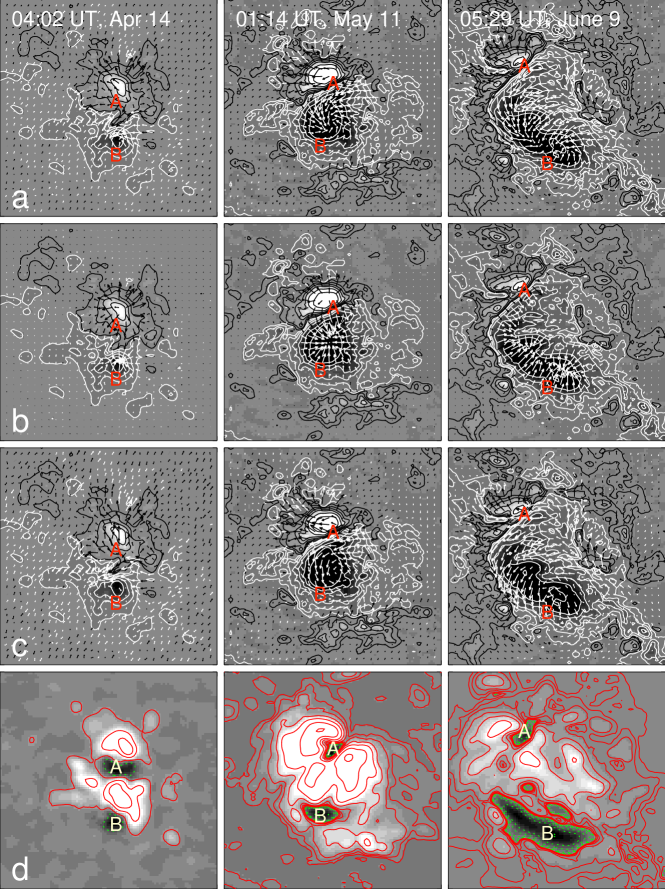
Figure 2.: The vector magnetic fields in Active Regions NOAA 6580 (N28, W12) on April 14, 1991 (left), NOAA 6619 (N29, E09) on May 11, 1991 (middle) and NOAA 6659 (N32, E05) on June 9, 1991 (right). Top row (a): The arrows mark the observed transverse component of field ${\bf B}_{o}$. Second row (b): The arrows show the transverse components of the potential field ${\bf B}_{p}$ inferred from the longitudinal components of observational magnetic fields. Third row (c): The arrows show the transverse components of the non-potential field ${\bf B}_{n}$ inferred from Equation (eq:MGshear). The contours indicate the longitudinal magnetic field distribution of $\pm$50, 200, 500, 1000, 1800, and 3000 G. Bottom row (d): The contours show the distribution of free magnetic energy densities $\rho_{fh}$ of $\pm$1, 5, 10, 20, 50, 100, 200, and 400$\times 10^{3}$ (Mx²cm${}^{-4})$ for the quantity shown in gray scale, where solid (dashed) lines correspond to positive (negative) sign.Fig:nonpoten

Figure 3.: A schematic of the development of Active Region NOAA 6580-6619-6659 in June 1991, and also the relationship among the observed magnetic field ${\bf B}_{o}$, the potential field ${\bf B}_{p}$, and the non-potential field ${\bf B}_{n}$ as viewed from above. fig:MGsh1

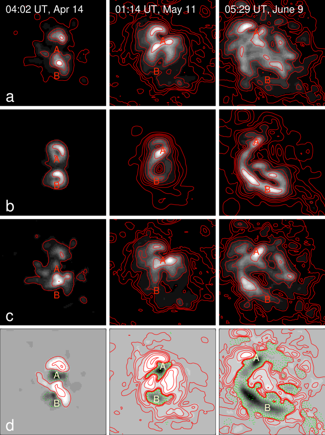
Figure 4.: The magnetic energy density parameters in Active Region NOAA 6580 on April 14, 1991 (left), NOAA 6619 on May 11, 1991 (middle), and NOAA 6659 on June 9, 1991 (right). Top row (a): Inferred from the observed transverse component of field ${\bf B}_{o}$. Second row (b): Inferred from the the transverse components of potential field ${\bf B}_{p}$ calculated by the longitudinal components of observed magnetic fields. Third row (c): Inferred from the transverse components of non-potential field ${\bf B}_{n}$. Bottom row (d): The difference $\frac{1}{4\pi}{\bf B}_{nh}\cdot{\bf B}_{ph}$ between magnetic free energy density $\rho_{fh}$ and the energy density of the non-potential field $\rho_{nh}$ in Equetion (eq:enegcomp1). The contours indicate $\pm$1, 5, 10, 20, 50,100, 200, and 400$\times 10^{3}$ (Mx² cm^-4) for the quantity shown in gray scale, where solid (dashed) lines correspond to positive (negative) sign.Fig:nonpotene

Figure Fig:nonpoten also shows the relationship among the observed highly twisted vector magnetic fields, the calculated potential and non-potential magnetic fields, and the corresponding magnetic free energy densities in the super active region NOAA 6580-6619-6659 in 1991. We can find in row (a) of Figure Fig:nonpoten that highly twisted transverse magnetic fields form in the active region. Row (b) of Figure Fig:nonpoten shows the calculated transverse components of potential magnetic fields inferred by the observed longitudinal magnetic fields of the active region. Row (c) of Figure Fig:nonpoten shows the non-potential components of magnetic fields inferred by Equation (eq:MGshear). In row (d) of Figure Fig:nonpoten, the magnetic free energy densities in the active region are inferred by $\rho_{fh}$ in Equation (eq:MGsh0) to be contributed by the transverse components of fields alone. We find that the free energy density is negative in some areas (highly sheared magnetic neutral lines) of the active region, i.e. $(\frac{1}{8\pi}{B}_{nh}^{2}+\frac{1}{4\pi}{\bf B}_{nh}\cdot{\bf B}_{ph})<0$ in Equation (eq:MGsh00), where ${\bf B}_{ph}$ is inferred by the observed longitudinal magnetic field. These areas of negative sign, labeled $A$ and $B$, can be defined as negative energy regions in row (d) of Figure Fig:nonpoten.

Figure fig:MGsh1 shows a schematic of the development process of the observed highly twisted vector magnetic field in the super active region NOAA 6580-6619-6659 in 1991. With the emergence of the new magnetic flux, the highly sheared magnetic field formed near the magnetic neutral line of the active region, and the transverse component of the magnetic fields gradually became parallel to the magnetic neutral line. This relates to the storage of free magnetic energy and the formation of ‘negative energy regions’ in the active region.

Figure fig:MGsh1 also shows the relationship among the observed magnetic field ${\bf B}_{o}$, the potential field ${\bf B}_{p}$, and the non-potential field ${\bf B}_{n}$ near the magnetic neutral line in the active region as viewed from above. This provides a possibility for the occurrence of negative energy regions in the active regions as $\frac{1}{8\pi}{B}_{n}^{2}<-\frac{1}{4\pi}{\bf B}_{n}\cdot{\bf B}_{p}$. The relevant results can be found in Figure Fig:nonpotend. We can find that in these negative energy regions the inclined angles $\varphi$ between the potential and non-potential components of transverse fields in the active region are larger than 90^∘, i.e. $\frac{1}{4\pi}{\bf B}_{n}\cdot{\bf B}_{p}$ is negative in Figures Fig:nonpoten and fig:MGsh1.

For comparison, Figure Fig:nonpotene shows the distribution of different types of magnetic energy density parameters in Active Region NOAA 6580-6619-6659 in 1991. In the calculation of the photospheric energy density, only transverse components of the magnetic fields were used because the longitudinal components do not change in this analysis. Row (a) of Figure Fig:nonpotene shows the magnetic energy densities inferred from the observational transverse magnetic fields. Row (b) of Figure Fig:nonpotene shows the magnetic energy density inferred from the potential transverse magnetic fields, which is calculated using only the longitudinal components of magnetic fields. Row (c) of Figure Fig:nonpotene shows the energy density parameters $\rho_{n}$ of non-potential magnetic fields.

There are obvious differences among the magnetic energy density parameters inferred from the observational transverse components of fields ${\bf B}_{oh}$, from the potential transverse components of field ${\bf B}_{ph}$, and from the non-potential transverse components of field ${\bf B}_{nh}$. We note that row (d) of Figure Fig:nonpotene shows the difference $\frac{1}{4\pi}{\bf B}_{nh}\cdot{\bf B}_{ph}$ between the magnetic energy density $\rho_{fh}$ (Equation (eq:MGsh0)) and the energy density parameter $\rho_{n}$ of the non-potential transverse magnetic fields in Equation (Eq-fED). The large-scale negative sign areas $A$ and $B$ reflect where components of the potential field show large inclination angles to the non-potential field in Active Region NOAA 6580-6619-6659.

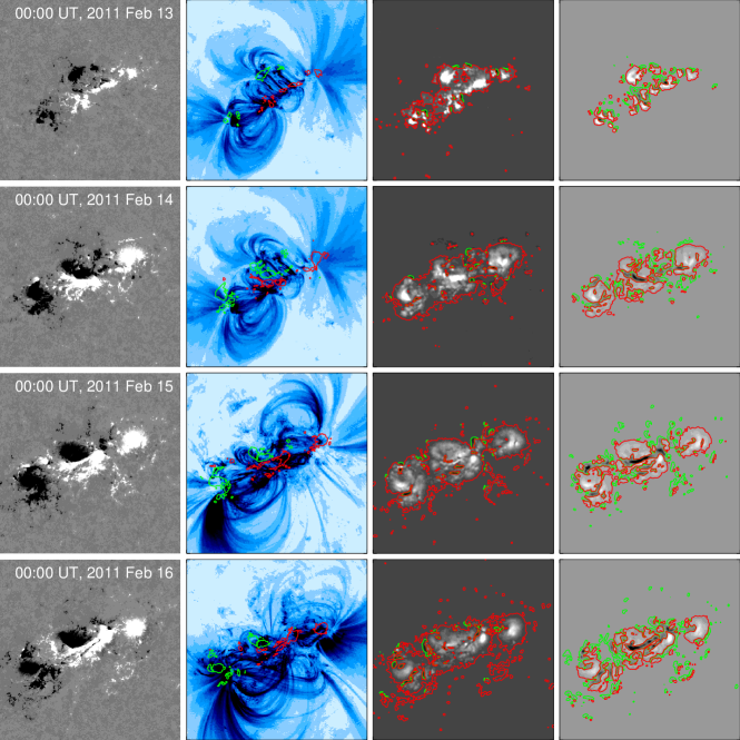
Figure 5.: Active Region NOAA 11158 in February 2011 at four different times. From left to right: the longitudinal magnetic fields, 171 Å images overlaid with contours of $\pm 10^{3}$ G magnetic fields, the magnetic free energy density $\rho_{fh}$, and the quantity $\frac{1}{4\pi}{\bf B}_{nh}\cdot{\bf B}_{ph}$. The contours of the magnetic energy densities indicate $\pm 10^{3}$ (Mx² cm^-4). The red (green) contours refer to the positive (negative) sign. Fig:magene11158

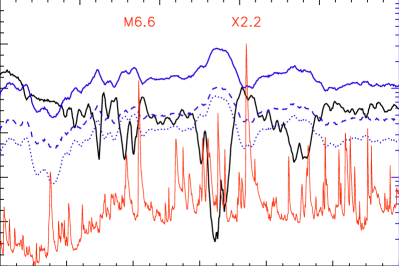
Figure 6.: The evolution of mean magnetic energy density parameters in Active Region NOAA 11158 in February 2011. The blue solid line ($\overline{B_{oh}^{2}/8\pi}$) is calculated based on the observational photospheric transverse field, the blue dotted line ($\overline{B_{ph}^{2}/8\pi}$) is the calculated transverse potential field, and the blue dashed line is the $\overline{\rho_{nh}}=\overline{B_{nh}^{2}/8\pi}$ inferred from the transverse non-potential field, while the black solid line shows the corresponding $\overline{\frac{1}{4\pi}{\bf B}_{nh}\cdot{\bf B}_{ph}}$. The red line shows the GOES flux. Fig:enelines11158

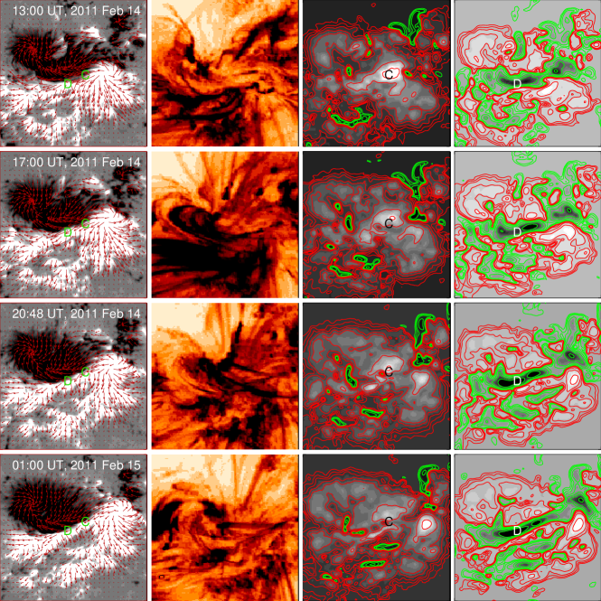
Figure 7.: A local area of Active Region NOAA 11158 in February 14-15, 2011. From left to right: longitudinal magnetic fields, 171 Å images, magnetic free energy density $\rho_{fh}$, and the quantity $\frac{1}{4\pi}{\bf B}_{nh}\cdot{\bf B}_{ph}$. The contours of the magnetic energy density indicate $\pm$1, 5, 10, 20, 50, 100, 200, and 400$\times 10^{3}$ (Mx² cm^-4). The red (green) contours refer to the positive (negative) sign. Fig:maen11158-14-15

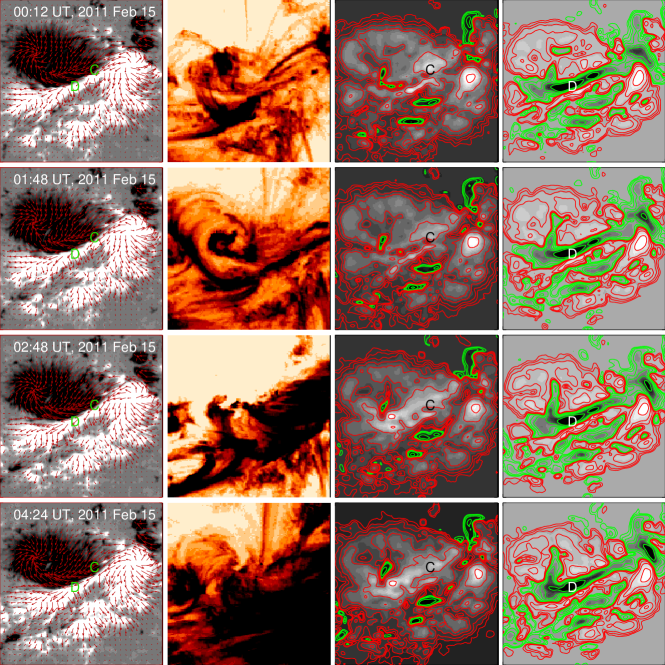
Figure 8.: A local area of Active Region NOAA 11158 on February 15, 2011. From left to right: longitudinal magnetic fields, 171Å images, magnetic free energy density $\rho_{fh}$, and the difference quantity $\frac{1}{4\pi}{\bf B}_{nh}\cdot{\bf B}_{ph}$. The contours of the magnetic energy density indicate $\pm$1, 5, 10, 20, 50, 100, 200, and 400$\times 10^{3}$ (Mx² cm^-4). The red (green) contours refer to the positive (negative) sign. Fig:maen11158-15

3.2 Active Region NOAA 11158

It is notable that vector magnetic field data have been made available with the Helioseismic and Magnetic Imager (HMI) instrument (Schou et al., 2012) onboard the Solar Dynamics Observatory (SDO). Active Region NOAA 11158 is a notable active region observed by HMI. A series of articles has focused on the development of magnetic fields and solar flares and CMEs in Active Region NOAA 11158 based on observational vector magnetograms and EUV images (cf. Aschwanden et al., 2014; Bamba et al., 2013; Chintzoglou and Zhang, 2013; Dalmasse et al., 2013; Gary et al., 2014; Gosain, 2012; Guerra et al., 2015; Inoue et al., 2013; Jiang et al., 2012; Jing et al., 2012; Liu and Schuck, 2012; Maurya et al., 2012; Malanushenko et al., 2014; Kazachenko et al., 2015; Petrie, 2012; Song et al., 2013; Su et al., 2012; Tarr et al., 2013; Toriumi et al., 2013; Tziotziou et al., 2013; Vemareddy et al., 2012a, b; Wang et al., 2012, 2013; Yang et al., 2014; Zhao et al., 2014; Zhang et al., 2014). The development of photospheric vector magnetic fields in the active region with flares and CMEs is also related to the basic question of the distribution of magnetic energy in the photosphere and the storage process of magnetic energy for the powerful flares and CMEs.

Fisher et al. (1998) found that the X-ray luminosity shows the best correlation with the total unsigned magnetic flux. Similarly, Fludra and Ireland (2008) reported EUV emission to be linearly related to the amount of magnetic flux, regardless of potentiality. Figure Fig:magene11158 shows the distribution of magnetic field, 171Å images, free magnetic energy density $\rho_{fh}$ (Equation (eq:MGsh0)) and the difference $\frac{1}{4\pi}{\bf B}_{nh}\cdot{\bf B}_{ph}$ between magnetic energy density $\rho_{fh}$ and energy density parameter $\rho_{n}$ (Equation (Eq-fED)) of the non-potential magnetic field. Similar to Active Region NOAA 6580-6619-6659, we also find some small-scale negative sign areas of free magnetic energy density in Active Region NOAA 11158.

Figure Fig:enelines11158 shows the evolution of the mean values of different energy parameters of Active Region NOAA 11158 with the GOES flux inferred from a series of vector magnetograms in the period of February 12-16, 2015. It is found that the mean magnetic free energy density $\overline{\rho_{fh}}$ (Equation (eq:MGsh0)), the mean energy density parameter $\overline{\rho_{nh}}$ (Equation (Eq-fED)) of the non-potential magnetic field, and the mean potential energy density in Active Region NOAA 11158 in February 2011 show almost the same evolution tendency. The photospheric mean magnetic energy densities of the active region tend to decrease before the X-ray M6.6 flare on February 13 and the X2.2 flare on February 15. Furthermore, the difference $\overline{\frac{1}{4\pi}{\bf B}_{nh}\cdot{\bf B}_{ph}}$ (between the mean magnetic free energy density $\overline{\rho_{fh}}$ and the mean energy density parameter $\overline{\rho_{nh}}$ of the non-potential magnetic field) shows the opposite trend relative to others. This suggests the possibility that some amount of free magnetic energy is stored in the lower solar atmosphere before powerful flares. This is also consistent with the release of free magnetic energy driving powerful flares. Moreover, the limitations on the time resolution of the magnetic field observations should also be noted, for example, HMI vector magnetograms incorporate data integrated over 1215 seconds etc. (Liu et al., 2012b), which implies that some changes do not provide sufficient evidence to show if the evolution of the magnetic field actually precedes the flares.

Figure Fig:maen11158-14-15 shows the evolution of the vector magnetic field, 171 Å images, magnetic free energy density $\rho_{fh}$ and the difference quantity $\frac{1}{4\pi}{\bf B}_{nh}\cdot{\bf B}_{ph}$ in the middle of Active Region NOAA 11158 to analyze the evolution of these quantities before the X2.2 flare on February 15. The large-scale negative energy density parameter $\frac{1}{4\pi}{\bf B}_{nh}\cdot{\bf B}_{ph}$ tends to extend along the direction of EUV 171 Å loops and the highly sheared major magnetic neutral line between large-scale opposite polarities in the active region. As compared with the evolution of the magnetic energy density, it is found that the maximum value of the free magnetic energy density $C$ weakens, and the channel where $\frac{1}{4\pi}{\bf B}_{nh}\cdot{\bf B}_{ph}$ is negative (marked by $D$) tends to increase near the magnetic neutral line in the Active Region NOAA 11158 before the X2.2 flare.

Figure Fig:maen11158-15 shows the change in the vector magnetic fields, 171 Å images, magnetic free energy density $\rho_{fh}$, and the difference quantity $\frac{1}{4\pi}{\bf B}_{nh}\cdot{\bf B}_{ph}$ in the local area of Active Region NOAA 11158 from 90 minutes before the X2.2 flare (start at 01:44, peak at 01:45, end at 01:56 UT) to after on February 15, 2011. The eruption of EUV 171 Å loops occurred near the highly sheared magnetic neutral line and also above the extreme negative $\frac{1}{4\pi}{\bf B}_{nh}\cdot{\bf B}_{ph}$ area.

For a detailed analysis, Figure Fig:nonpotene11158e shows the relationship between the vector magnetic field and different energy parameters in Active Region NOAA 11158 at 00:12 UT on February 15, 2011. Figures Fig:nonpotene11158eb and Fig:nonpotene11158ec show the magnetic free energy density $\rho_{fh}$ (Equation (eq:MGsh0)) and the energy density parameter $\rho_{nh}$ (Equation (Eq-fED)) of non-potential magnetic field in Active Region NOAA 11158 in February 2011, respectively. Figure Fig:nonpotene11158ed shows $\frac{1}{4\pi}{\bf B}_{nh}\cdot{\bf B}_{ph}$ overlaid with 171 Å images. The large-scale extreme negative value of $\frac{1}{4\pi}{\bf B}_{nh}\cdot{\bf B}_{ph}$ tends to form along the direction of EUV 171 Å loops and the highly sheared magnetic major neutral line between large-scale opposite polarities in the active region. This is important for understanding the distribution of magnetic energy above the solar surface.

Figure Fig:nonpotene11158f shows the relationship between the energy density parameter $\frac{1}{4\pi}{\bf B}_{nh}\cdot{\bf B}_{ph}$ and the different components of the vector magnetic field in the local area of Figure Fig:nonpotene11158e in Active Region NOAA 11158. It also shows that negative-sign areas of $\frac{1}{4\pi}{\bf B}_{nh}\cdot{\bf B}_{ph}$ formed near the magnetic neutral lines with highly sheared transverse magnetic fields, where the most significant difference between the non-potential and potential fields can be found.

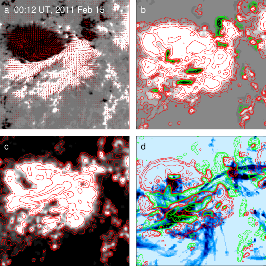
Figure 9.: (a) The vector magnetic field in Active Region NOAA 11158 on February 15, 2011. (b) The magnetic free energy density $\rho_{fh}$ (Equation (eq:MGsh0)) and (c) the energy density of the non-potential magnetic field $\rho_{n}$ (Equation (Eq-fED)) in Active Region NOAA 11158. (d) The difference $\frac{1}{4\pi}{\bf B}_{nh}\cdot{\bf B}_{ph}$ (between the magnetic free energy density $\rho_{fh}$ and the energy density parameter $\rho_{nh}$ (Equation (eq:enegcomp1)) of the non-potential magnetic field) overlaid with the AIA 171 Å image. The contours indicate the magnetic energy density of $\pm$1, 5, 10, 20, 50, 100, 200, and 400$\times 10^{3}$ (Mx² cm^-4), where red (green) contours refer to the positive (negative) sign. Fig:nonpotene11158e

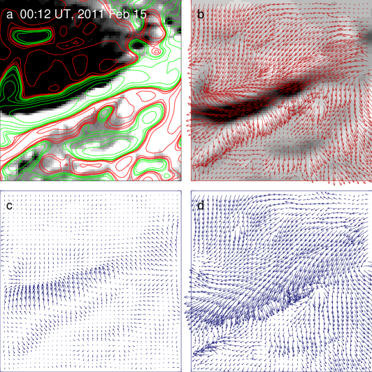
Figure 10.: (a) A local area of longitudinal magnetic field (gray scale) and the corresponding $\frac{1}{4\pi}{\bf B}_{n}\cdot{\bf B}_{p}$ (contours) in Active Region NOAA 11158 on February 15, 2011 near the center of Figure Fig:nonpotene11158e. The contours indicate the magnetic energy density of $\pm$1, 5, 10, 20, 50, 100, 200, and 400$\times 10^{3}$ (Mx²cm^-4), where red (green) contours refer to the positive (negative) sign. (b) The $\frac{1}{4\pi}{\bf B}_{n}\cdot{\bf B}_{p}$ (gray scale) and the corresponding observed transverse magnetic field. (c) The corresponding potential component and (d) the non-potential component of the transverse field. Fig:nonpotene11158f

In addition to the analysis of other magnetic parameters, such as magnetic flux near neutral lines (e.g. Schrijver, 2007) and integrated unsigned vertical current density (e.g. Sun et al., 2012), Figure Fig:maen11158-curhel shows the distribution of the vertical current (${\bf J}_{z}$) and current helicity density ($(\nabla\times{\bf B})_{z}\cdot{\bf B}_{z}$) in the middle of Active Region NOAA 11158 inferred from observed vector magnetograms with the comparison of the magnetic free energy density $\rho_{fh}$ and the difference quantity $\frac{1}{4\pi}{\bf B}_{nh}\cdot{\bf B}_{ph}$. These magnetic energy parameters are presented in Figure Fig:maen11158-14-15 with the relevant discussions. We can find that the magnetic energy parameters show obvious different density distributions relative to the current and current helicity densities because energy parameters reflect the storage of magnetic energy in the solar atmosphere, while the current and current helicity density provide information on the twist and handedness of magnetic fields in active regions. These show different aspects of magnetic lines of force in solar active regions, even though they are also important quantities in the analysis of solar eruptive activities. Moreover, the development of the vector magnetic field and its relationship with helicities and spectrums in the active region are discussed by Zhang et al. (2014, 2016).

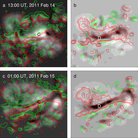
Figure 11.: The vertical current (${\bf J}_{z}$) and current helicity density ($h_{z}=(\bigtriangledown\times{\bf B})_{z}\cdot{\bf B}_{z}$) in Active Region NOAA 11158 on February 14, 2011 (top) and February 15, 2011 (bottom). The contours in the left panels (a and c) indicate the vertical current density of $\pm$5, 10, 20, and 50$\times 10^{-7}$ (A² cm^-2). The contours in the right panels (b and d) indicate the current helicity density $h_{z}$ of $\pm$5, 10, 20, 50, 100, and 200$\times 10^{-4}$ (G² cm^-1). The red (green) contours refer to the positive (negative) sign. The gray scale shows the corresponding magnetic free energy density $\rho_{fh}$ (left) and difference quantity $\frac{1}{4\pi}{\bf B}_{nh}\cdot{\bf B}_{ph}$ (right) shown in Figure Fig:maen11158-14-15. Fig:maen11158-curhel

4 Conclusion and Discussions

We have presented the magnetic energy density parameters inferred from photospheric vector magnetograms of the recurrent Active Region NOAA 6580-6619-6659 and 11158. This provided the opportunity of analyzing the storage and evolution of magnetic energy in active regions. After this analysis, the main results are as follows.

1) Observations of photospheric vector magnetic fields provide important information on the distribution of the free magnetic energy density in the lower solar atmosphere. The free magnetic energy density is comprised of the two terms $\frac{1}{8\pi}{B}_{nh}^{2}$ and $\frac{1}{4\pi}{\bf B}_{nh}\cdot{\bf B}_{ph}$. The first term refers to non-potential magnetic fields and the second to the relationship between the non-potential and potential fields. This means that the change in the photospheric free magnetic energy density not only depends on the non-potential component of magnetic field but also on the relationship with the potential field.

2) The term $\frac{1}{4\pi}{\bf B}_{nh}\cdot{\bf B}_{ph}$ is an important quantity for understanding the degree of magnetic shear in the active regions. The negative sign of $\frac{1}{4\pi}{\bf B}_{nh}\cdot{\bf B}_{ph}$ tends to occur in areas of highly sheared magnetic fields in the active regions. Moreover, in the strongly sheared areas $(\frac{1}{8\pi}{B}_{nh}^{2}+\frac{1}{4\pi}{\bf B}_{nh}\cdot{\bf B}_{ph})<0$ relative to the highly sheared magnetic fields defined as a negative energy region can form in delta active regions. If the inclination angles between potential and non-potential magnetic lines of force decrease with height in the solar atmosphere of the active regions, the term $\frac{1}{4\pi}{\bf B}_{nh}\cdot{\bf B}_{ph}$ will change sign from negative to positive with the increase of height near the magnetic neutral lines in the active regions. This is consistent with the idea that some free magnetic energy is stored in the high solar atmosphere of active regions where powerful flares might be triggered. The trigger of powerful flares and CMEs in active regions, such as NOAA 6659 and 11158, was analyzed by some authors (cf. Schmieder et al., 1994; Zhang et al., 1994; Yan and Wang, 1995; Wang, 1997; Choudhary, 2000; Liu et al., 2012a; Schrijver et al., 2011; Sun et al., 2012; Chintzoglou and Zhang, 2013; Jiang and Feng, 2013; Shen et al., 2013; Sorriso-Valvo et al., 2015). A very simplifed picture on the relationship $\frac{1}{4\pi}{\bf B}_{nh}\cdot{\bf B}_{ph}$ with height in active regions is shown in Figure Fig:shearv.

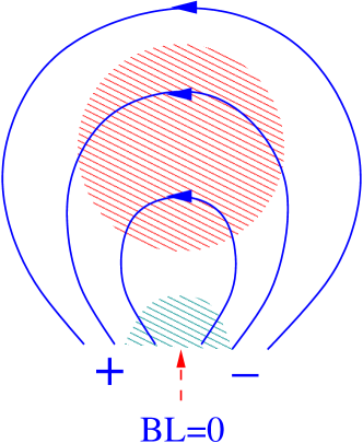
Figure 12.: A simplified schematic of $\frac{1}{4\pi}{\bf B}_{nh}\cdot{\bf B}_{ph}$ with height above the photospheric magnetic neutral line in the highly sheared active region as viewed from the side. The red (blue) shade shows the positive (negative) sign area. The red arrow indicates the photospheric magnetic neutral line in the active region.Fig:shearv

3) The mean photospheric magnetic energy in the active regions obviously changes before some powerful solar flares. This might reflect the release of stored free magnetic energy powering flares, even if the free energy density can be negative in the photosphere in localized areas of some active regions.

From the analysis of the magnetic energy density of active regions in the lower solar atmosphere, we would like to discuss the following questions.

The analysis of magnetic shear in active regions is normally based on the inclination angle between the observed and the potential transverse magnetic field. The magnetic shear provides some information about the triggering of solar flares and CMEs, although it cannot provide all information about the free magnetic energy in flare- or CME-producing regions even in the lower solar atmosphere because the real configuration of the magnetic fields in active regions is more complex.

The transverse and longitudinal components of the magnetic fields are inferred from the Stokes parameters Q, U, and V, respectively, with different calibration coefficients. The accuracy of the measurements of different components of the vector magnetic fields is still a basic problem for determining the photospheric free magnetic energy density in solar active regions.

It should be noted that the transverse potential field is a fictitious quantity inferred from the observational longitudinal field, so that its strength is a reference value in calculating the magnetic energy density of active regions in the photosphere. The transverse components of potential magnetic fields can be calculated by the extrapolating the longitudinal components of the observed magnetic fields. The estimation of the non-potential components of the fields also obviously depends on the measured longitudinal fields and on the choice of extrapolation methods for the horizontal components of the potential fields.

Acknowledgments

The author would like to thank the anonymous referee for the suggestions and comments that helped improve the manuscript. This study is supported by grants from the National Natural Science Foundation (NNSF) of China under the project grants 10921303, 11221063, 11673033 and 41174153.

References

- Ai and Hu (1986) Ai, G., Hu, Y., 1986, Pub. Bei. Obs., 8, 1.
- Aschwanden et al. (2014) Aschwanden, M., Sun, X., Liu, Y., 2014, ApJ, 785, 34.
- Bamba et al. (2013) Bamba, Y., Kusano, K., Yamamoto, T. T., Okamoto, T. J., 2013, ApJ, 778, 48.
- Bumba et al. (1993) Bumba, V., Klvana, M., Kalman, B., Gyori, L., 1993, A&A, 276, 193.
- Chandrasekhar (1961) Chandrasekhar, S., 1961, Hydrodynamic and hydromagnetic stability, Clarendon Press.
- Chen et al. (1989) Chen, J., Ai, G., Zhang, H., Jiang, S., 1989, Pub. Yun. Obs., 1S, 108.
- Chintzoglou and Zhang (2013) Chintzoglou, G., Zhang, J., 2013, ApJ, 764, L3.
- Choudhary (2000) Choudhary, D., 2000, Ap&SS, 274, 463.
- Dalmasse et al. (2013) Dalmasse, K., Pariat, E., Valori, G., Démoulin, P., Green, L. M., 2013, A&A, 555, L6.
- Fisher et al. (1998) Fisher, G. H., Longcope, D. W., Metcalf, T. R., Pevtsov, A. A., 1998, ApJ, 508, 885.
- Fludra and Ireland (2008) Fludra, A., Ireland, J., 2008, A&A, 483, 609.
- Gary et al. (2014) Gary, G. Allen, Hu, Q., Lee, J., Aschwanden, M., 2014, Sol. Phys., 289, 3703.
- Gosain (2012) Gosain, S., 2012, ApJ, 749, 85.
- Guerra et al. (2015) Guerra, J. A., Pulkkinen, A., Uritsky, V. M., Yashiro, S., 2015, Sol. Phys., 290, 335.
- Hagyard and Teuber (1978) Hagyard, M. J., Teuber, D., 1978, Sol. Phys., 57, 267.