NOETHER SYMMETRIES AND INTEGRABILITY IN TIME-DEPENDENT HAMILTONIAN MECHANICS

Abstract.

We consider Noether symmetries within Hamiltonian setting as transformations that preserve Poincaré–Cartan form, i.e., as symmetries of characteristic line bundles of nondegenerate 1-forms. In the case when the Poincaré–Cartan form is contact, the explicit expression for the symmetries in the inverse Noether theorem is given. As examples, we consider natural mechanical systems, in particular the Kepler problem. Finally, we prove a variant of theorem on the complete (non-commutative) integrability in terms of Noether symmetries of time-dependent Hamiltonian systems.

1. Introduction

1.1.

Since Emmy Noether’s paper [27] on integrals related to invariant variational problems, there has been a lot of efforts on its generalization, geometrical formulation, as well as on the application in various concrete problems (e.g, see [23, 29]). For finite dimensional Lagrangian systems, Noether’s general statement [27] takes the following simple form.

Consider a Lagrangian system $(Q,L)$, where $Q$ is a configuration space and $L(t,q,\dot{q})$ is a Lagrangian, $L:\mathbb{R}\times TQ\to\mathbb{R}$. Let $q=(q_{1},\dots,q_{n})$ be local coordinates on $Q$. The motion of the system is described by the Euler–Lagrange equations

(1.1) $$\frac{d}{dt}\frac{\partial L}{\partial\dot{q}_{i}}=\frac{\partial L}{\partial q_{i}},\quad i=1,\dots,n.$$

One of the basic principles of classical mechanics, the Hamiltonian principle of least action, or the principle of stationary action, says that the solutions of the Euler–Lagrange equations are the critical points of the action integral

(1.2) $$S_{L}({\gamma})=\int_{a}^{b}L(t,q,\dot{q})dt$$

in a class of curves ${\gamma}:[a,b]\to Q$ with fixed endpoints ${\gamma}(a)=q_{0}$, ${\gamma}(b)=q_{1}$ (e.g., see [2, 9, 18, 21, 35]).

Consider the action of an one-parameter group of diffeomorphisms $g_{s}$ on $\mathbb{R}\times Q$ with the induced vector field $\nu=(\tau,\xi)|_{(t,q)}=\frac{d}{ds}|_{s=0}g_{s}(t,q)$. After prolongation to $\mathbb{R}\times TQ$, the induced vector field reads

(1.3) $$\hat{\nu}=\tau(t,q)\frac{\partial}{\partial t}+\sum_{i}\xi^{i}(t,q)\frac{\partial}{\partial q_{i}}+{\hat{\xi}}^{i}(t,q,\dot{q})\frac{\partial}{\partial\dot{q}_{i}},$$

where (e.g., see [4, 11])

$${\hat{\xi}}^{i}=\frac{\partial\xi^{i}}{\partial t}-\dot{q}_{i}\frac{\partial\tau}{\partial t}+\sum_{j}\big{(}\frac{\partial\xi^{i}}{\partial q_{j}}\dot{q}_{j}-\dot{q}_{i}\frac{\partial\tau}{\partial q_{j}}\dot{q}_{j}\big{)}.$$

The group $g_{s}$ is a Noether symmetry of the Lagrangian system if it preserves the action functional (1.2), that is, if

(1.4) $$\frac{\partial L}{\partial t}\tau+\sum_{i}{\big{(}\frac{\partial L}{\partial q_{i}}\xi^{i}+\frac{\partial L}{\partial\dot{q}_{i}}{\hat{\xi}}^{i}\big{)}}+L\big{(}\frac{\partial\tau}{\partial t}+\sum_{j}\frac{\partial\tau}{\partial q_{j}}\dot{q}_{j}\big{)}=0.$$

The Noether theorem says that if $g_{s}$ is a Noether symmetry then

$$I(t,q,\dot{q})=\frac{\partial L}{\partial\dot{q}}(\xi-\tau\dot{q})+L\tau=\sum_{i}{\frac{\partial L}{\partial\dot{q}_{i}}(\xi^{i}-\tau\dot{q}_{i})}+L\tau$$

is the first integral of the Euler-Lagrange equations. More generally, if we have the invariance of (1.2) modulo the integral of ${df}/{dt}$ , that is at the right hand side of (1.4) we have ${df}/{dt}$, for some function $f(t,q)$ (so called gauge term), then the integral is $I(t,q,\dot{q})-f(t,q)$.

Two cases are of particular interest. If $\tau\equiv 0$ then (1.4) reduces to the condition that the Lagrnagian $L$ is invariant with respect to $g_{s}$,

$$\sum_{i}{\frac{\partial L}{\partial q_{i}}\xi^{i}+\frac{\partial L}{\partial\dot{q}_{i}}{\hat{\xi}}^{i}}=0,$$

and the Noether integral takes the basic form

$$I(t,q,\dot{q})=\frac{\partial L}{\partial\dot{q}}(\xi)=\sum_{i}\frac{\partial L}{\partial\dot{q}_{i}}\xi^{i}.$$

In particular, when the Lagrangian does not depend on $q_{1}$, then $q_{1}$ is ignorable (cyclic) coordinate and the integral is ${\partial L}/{\partial\dot{q}_{1}}$ (e.g, see [2, 35]).

Secondly, if the Lagrangian does not depend on time, we can take the translations in time: $g_{s}(t,q)=(t+s,q)$. Then the vector field (1.3) is simply ${\partial}/{\partial t}$ and the integral $I$ becomes the energy of the system multiplied by $-1$:

$$I=-E=-\sum_{i}{\frac{\partial L}{\partial\dot{q}_{i}}\dot{q}_{i}}+L.$$

1.2.

The Noether theorem can be seen as a part of time-dependent mechanics that is studied and geometrically formulated both in the Lagrangian and Hamiltonian setting (e.g., see [1, 3, 6, 8, 10, 11, 12, 13, 25, 26, 24, 31, 32] and references therein). In Sarlet and Cantrijn [4], one can find a review of various approaches on the Noether theorem in the Lagrangian framework for velocity dependent transformations, as well as a geometrical setting for the equivalence of the first integrals and symmetries of the Lagrangian system considered as a characteristic system of the two-form $d\alpha$ ($\alpha$ being Poincaré–Cartan form).

The aim of this paper is to present the problem through the perspective of contact geometry, continuing the study of the Maupertuis principle, isoenergetic, and partial integrability [18, 19]. We consider Noether symmetries as symmetries of characteristic line bundles of nondegenerate 1-forms (Theorems 2.1, 3.2). In the case of time-dependent Hamiltonian systems, Noether symmetries are transformations that preserve Poincaré–Cartan form (see Proposition 2.1), and, via Legendre transformation, this is equivalent to Crampin’s notion of symmetry of Lagrangian systems [10]. This will allow us to use contact geometry for the inverse Noether theorem in Section 4.

The notion of a weak Noether symmetry is also given and the relation with the Noether symmetries is established (Proposition 4.1). The Noether symmetry is a natural generalization of classical Noether symmetry described above (see Proposition 2.2), while the notion of the week Noether symmetry corresponds to the classical Noether symmetry with the gauge term.

In the case when the Poincaré–Cartan form is contact, the explicit expression for the Noether symmetry for a given first integral without using the gauge term is given (Theorem 4.1). As examples, we consider natural mechanical systems (Corollary 4.1), in particular the Kepler problem (Example 4.3).

Finally, in Section 5, we obtain a variant of the complete (non-commutative) integrability in terms of Noether symmetries of time-dependent Hamiltonian systems (Theorem 5.1, Corollary 5.1).

2. Noether symmetries in the Hamiltonian formulation

2.1.

Let $(Q,L)$ be a Lagrangian system. The Legendre transformation $\mathbb{F}L:TQ\to T^{*}Q$ is defined by

(2.1) $$\mathbb{F}L(t,q,\xi)\cdot\eta=\frac{d}{ds}|_{s=0}L(t,q,\xi+s\eta)\quad\Longleftrightarrow\quad p_{i}=\frac{\partial L}{\partial\dot{q}_{i}},\quad i=1,\dots,n,$$

where $\xi,\eta\in T_{q}Q$ and $(q_{1},\dots,q_{n},p_{1},\dots,p_{n})$ are canonical coordinates of the cotangent bundle $T^{*}Q$. In order to have a Hamiltonian description of the dynamics we suppose that the Legendre transformation (2.1) is a diffeomorphism. The corresponding Lagrangian $L$ is called hyperregular [9].

Let $L(t,q,\dot{q})$ be a hyperregular Lagrangian. We can pass from velocities $\dot{q}_{i}$ to the momenta $p_{j}$ by using the standard Legendre transformation (2.1). In the coordinates $(q,p)$ of the cotangent bundle $T^{*}Q$, the equations of motion (1.1) read:

(2.2) $$\frac{dq_{i}}{dt}=\frac{\partial H}{\partial p_{i}},\qquad\frac{dp_{i}}{dt}=-\frac{\partial H}{\partial q_{i}},\qquad i=1,\dots,n,$$

where the Hamiltonian function $H(t,q,p)$ is the Legendre transformation of $L$

(2.3) $$H(t,q,p)=E(t,q,\dot{q})|_{\dot{q}=\mathbb{F}L^{-1}(t,q,p)}=\mathbb{F}L(t,q,\dot{q})\cdot\dot{q}-L(t,q,\dot{q})|_{\dot{q}=\mathbb{F}L^{-1}(t,q,p)}.$$

Let $pdq=\sum_{i}p_{i}dq_{i}$ be the canonical 1-form and

$$\omega=d(pdq)=dp\wedge dq=\sum_{i=1}^{n}dp_{i}\wedge dq_{i}$$

the canonical symplectic form of the cotangent bundle $T^{*}Q$. The equations (2.2) are Hamiltonian, i.e., they can be written as $\dot{x}=X_{H}$, where the Hamiltonian vector field $X_{H}$ is defined by

$$i_{X_{H}}\omega(\,\cdot\,)=\omega(X_{H},\,\cdot\,)=-dH(\,\cdot\,).$$

2.2. Noether symmetries

Consider the Poincaré–Cartan 1-form

$$\alpha=pdq-Hdt$$

on the extended phase space $\mathbb{R}\times T^{*}Q(t,q,p)$, where $H:\mathbb{R}\times T^{*}Q\to\mathbb{R}$ is a Hamiltonian function. The phase trajectories of the canonical equations (2.2) are extremals of the action

(2.4) $$A_{H}(\gamma)=\int_{\gamma}\alpha=\int_{\gamma}pdq-Hdt$$

in the class of curves $\gamma(t)=(t,q(t),p(t))$ connecting the subspaces $\{t_{0}\}\times T^{*}_{q_{0}}Q$ and $\{t_{1}\}\times T^{*}_{q_{1}}Q$ [2, 9] (Poincaré’s modification of the Hamiltonian principle of least action [30]). Obviously, we can replace $(T^{*}Q,dp\wedge dq)$ by an arbitrary exact symplectic manifold $(P,\omega=d\theta)$.

We shall say that the vector field

$$\zeta=\tau(t,q,p)\frac{\partial}{\partial t}+\sum_{i}{\xi^{i}(t,q,p)\frac{\partial}{\partial q_{i}}+\eta^{i}(t,q,p)\frac{\partial}{\partial p_{i}}},$$

i.e., the induced one-parameter group of diffeomeomorphisms $g_{s}^{\zeta}$ of $\mathbb{R}\times T^{*}Q$,

$$\zeta=\frac{d}{ds}g_{s}^{\zeta}|_{s=0}(t,q,p),$$

is a Noether symmetry of the Hamiltonian system (2.2) if the Poincaré–Cartan 1-form is preserved. Then, by the analogy with the Lagrangian formulation, $g_{s}^{\zeta}$ preserves the action functional (2.4). The above definition is suitable for a contact approach presented in Section 4.

We shall say that $\zeta$ is a weak Noether symmetry if we have the invariance of the perturbation of the Poincaré–Cartan 1-form 1-form by a closed 1-form $\beta$ modulo the differential of the function $f$:

(2.5) $$L_{\zeta}(pdq-Hdt+\beta)=df.$$

The function $f(t,q,p)$ plays a role of a gauge term in the classical formulation. The closed form $\beta$ corresponds to the fact that the solutions of the canonical equation (2.2) are also extremal of the perturbed action

$$A_{H}(\gamma)=\int_{\gamma}pdq-Hdt+\beta.$$

Theorem 2.1.

Let $\zeta$ be a waek Noether symmetry satisfying (2.5). Then

• The function

  $$J=i_{\zeta}(pdq-H\,dt+\beta)-f=\sum_{i}{p_{i}\xi^{i}}-H\tau+\beta(\zeta)-f$$

  is the first integral of the Hamiltonian equations (2.2).

• The integral $J$ is also preserved under the flow of $g_{s}^{\zeta}$.

• The one-parameter group of diffeomorphisms $g_{s}^{\zeta}$ permutes the trajectories of the Hamiltonian equations in the extended phase $\mathbb{R}\times T^{*}Q$ space modulo reparametrization.

The notion of week Noether symmetries for $\beta=0$ is equivalent, via Legendre transformation, to the symmetries of Lagrangin systems considered by Crampin [10], see also Sarlet and Cantrijn [4, 5]. The proof of Theorem 2.1 is similar to the proofs presented in [4, 5, 10] and for the completeness of the exposition it will be given in the next section (see the proof of Theorem 3.2). Also, recently, a similar approach to the higher order Lagrangian problems is given in [14].

By definition, $\zeta$ is a Noether symmetry if and only if the Lie derivative of the Poincaré–Cartan 1-form vanish:

$$0 =L_{\zeta}\alpha$$

$$=i_{\zeta}(d\alpha)+d(i_{\zeta}\alpha)$$

$$=i_{\zeta}(dp\wedge dq-dH\wedge dt)+d(p\xi-H\tau)$$

$$=\eta dq-\xi dp+\tau dH-dH(\zeta)dt+d(p\xi-H\tau)$$

$$=\eta dq+pd\xi-Hd\tau-dH(\zeta)dt.$$

Comparing the components with $dp_{j}$, $dq_{j}$, and $dt$ we get the following statement.

Proposition 2.1.

$\zeta$ is a Noether symmetry if and only if

(2.6) $$\sum_{i}p_{i}\frac{\partial\xi^{i}}{\partial p_{j}}-H\frac{\partial\tau}{\partial p_{j}}=0,$$

(2.7) $$\eta^{j}+\sum_{i}p_{i}\frac{\partial\xi^{i}}{\partial q_{j}}-H\frac{\partial\tau}{\partial q_{j}}=0,\qquad\qquad\quad j=1,\dots,n,$$

(2.8) $$\sum_{i}\big{(}p_{i}\frac{\partial\xi^{i}}{\partial t}-\eta^{i}\frac{\partial H}{\partial p_{i}}-\xi^{i}\frac{\partial H}{\partial q_{i}}\big{)}-H\frac{\partial\tau}{\partial t}-\tau\frac{\partial H}{\partial t}=0.$$

Proposition 2.2.

If the Lagrangian $L$ and the Hamiltonian $H$ are related by the Legendre transformation (2.1), (2.3) and if $\zeta$ is a Noether symmetry of the Hamiltonian equation (2.2) with $\xi^{i}=\xi^{i}(t,q)$, $\tau=\tau(t,q)$, then the classical invariance condition (1.4) is satisfied.

Proof.

Since $\xi^{i}$ and $\tau$ do not depend on $p$, the conditions (2.6) is satisfied. By expressing $\eta^{i}$ from (2.7) and substituting into (2.8) we get the following equation

(2.9) $$\sum_{j}p_{j}\big{(}\frac{\partial\xi^{j}}{\partial t}+\sum_{i}\frac{\partial\xi^{j}}{\partial q_{i}}\frac{\partial H}{\partial p_{i}}\big{)}- H\big{(}\frac{\partial\tau}{\partial t}+\sum_{j}\frac{\partial\tau}{\partial q_{j}}\frac{\partial H}{\partial p_{j}}\big{)}$$

$$-\sum_{j}\xi^{j}\frac{\partial H}{\partial q_{j}}-\tau\frac{\partial H}{\partial t}=0.$$

On the other hand, (1.4) transforms to

(2.10) $$\frac{\partial L}{\partial t}\tau+\sum_{i}\frac{\partial L}{\partial q_{i}}\xi^{i}+ \sum_{i}\frac{\partial L}{\partial\dot{q}_{i}}\big{(}\frac{\partial\xi^{i}}{\partial t}+\sum_{j}\frac{\partial\xi^{i}}{\partial q_{j}}\dot{q}_{j}\big{)}$$

$$-\big{(}\frac{\partial\tau}{\partial t}+\sum_{i}\frac{\partial\tau}{\partial q_{i}}\dot{q}_{i}\big{)}\big{(}\sum_{j}\frac{\partial L}{\partial\dot{q}_{j}}\dot{q}_{j}-L\big{)}=0.$$

Since the Legendre transformation (2.1), (2.3) implies well known identities

$$\frac{\partial L}{\partial t}=-\frac{\partial H}{\partial t},\qquad\frac{\partial L}{\partial q_{i}}=-\frac{\partial H}{\partial q_{i}},\qquad\dot{q}_{i}=\frac{\partial H}{\partial p_{i}},$$

the equations (2.9) and (2.10) are equivalent. ∎

Therefore, we can consider the above definition of a Noether symmetry as a natural generalization of the classical one.

3. Noether symmetries of characteristic line bundles

3.1.

Let $(M,\alpha)$ be a $(2n+1)$–dimensional manifold endowed with a nondegenerate 1-form $\alpha$. This mean that $d\alpha$ has the maximal rank $2n$. The kernel of $d\alpha$ defines one dimensional distribution

$$\mathcal{L}=\bigcup_{x}\mathcal{L}_{x},\qquad\mathcal{L}_{x}=\ker d\alpha|_{x}$$

of the tangent bundle $TM$ called characteristic line bundle. Also, at every point $x\in M$ we have the horizontal space $\mathcal{H}_{x}$ defined by

$$\mathcal{H}_{x}=\ker\alpha|_{x}.$$

In the case when $\alpha\neq 0$, $d\alpha\neq 0$ on $M$, then the collection of horizontal subspaces $\mathcal{H}=\bigcup_{x}\mathcal{H}_{x}=\bigcup_{x}\ker\alpha|_{x}$ is a nonintegrable distribution of $TM$, called horizontal distribution. If, in addition, $\alpha\wedge(d\alpha)^{n}\neq 0$, then $\alpha$ is a contact form and $(M,\alpha)$ is a strictly contact manifold [26]. The horizontal distribution $\mathcal{H}$ is also referred as contact distribution.

The following variational statement is well known.

Theorem 3.1.

The integral curves $\gamma:[a,b]\to M$ of the characteristic line bundle $\mathcal{L}$ are extremals of the action functional

$$A(\gamma)=\int_{\gamma}\alpha=\int_{a}^{b}\alpha(\dot{\gamma})dt$$

in the class of variations $\gamma_{s}(t)$, such that $\delta\gamma(a)$ and $\delta\gamma(b)$ are horizontal vectors.

Here, a variation of a curve $\gamma:[a,b]\to M$ is a mapping: $\Gamma:[a,b]\times[0,\epsilon]\to M$, such that $\gamma(t)=\Gamma(t,0)$, $t\in[a,b]$, $\delta\gamma(t)=\frac{\partial\Gamma}{\partial s}|_{s=0}\in T_{\gamma(t)}M$, and $\gamma_{s}(t)=\Gamma(t,s)$.

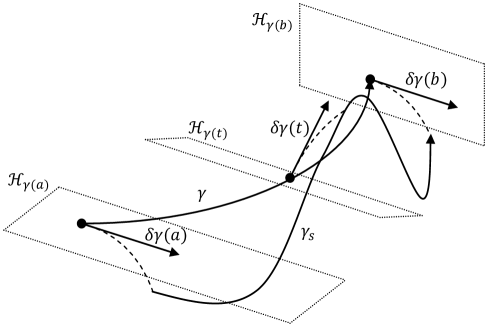
Figure 1. Variation of a curve $\gamma$, such that $\delta\gamma(a)$ and $\delta\gamma(b)$ are horizontal vectors.

The proof is a direct consequence of Cartan’s formula (e.g., see [16])

$$L_{\partial/\partial s}\Gamma^{*}\alpha|_{(t,0)}=\gamma^{*}(i_{\delta\gamma(t)}d\alpha)+d\gamma^{*}(\alpha(\delta\gamma(t))),$$

which implies

(3.1) $$\frac{d}{ds}\left(\int_{\gamma_{s}}\alpha\right)\bigg{|}_{s=0}=\int_{a}^{b}d\alpha(\delta\gamma(t),\dot{\gamma}(t))dt+\alpha(\delta\gamma(b))-\alpha(\delta\gamma(a)).$$

For $\delta\gamma(a)$ and $\delta\gamma(b)$ being horizontal, the expression (3.1) is equal to zero if and only if $\dot{\gamma}$ is in the kernel of the form $d\alpha$. That is, $\gamma(t)$ is an integral curve of the line bundle $\mathcal{L}$.

Example 3.1.

As an example we can take the extended phase space endowed with the Poincaré–Cartan 1-form

(3.2) $$(\mathbb{R}\times T^{*}Q(t,q,p),pdq-Hdt)$$

(e.g., see [2]). The sections of $\ker d(pdq-Hdt)$ are of the form

$$Z_{\mu}=\mu Z,$$

where

(3.3) $$Z=\frac{\partial}{\partial t}+\sum_{i}{\frac{\partial H}{\partial p_{i}}\frac{\partial}{\partial q_{i}}-\frac{\partial H}{\partial q_{i}}\frac{\partial}{\partial p_{i}}}.$$

and $\mu=\mu(t,q,p)$ are smooth functions. Therefore, in this case, Theorem 3.1 implies Hamiltonian principle of least action in the extended phase space. Here, the vector space $T^{*}_{q}Q$, considered as a subspace of $T_{(t,q,p)}\mathbb{R}\times T^{*}Q$, is a subspace of the horizontal space

(3.4) $$\mathcal{H}_{(t,q,p)}=\big{\{}\tau\frac{\partial}{\partial t}+\sum_{i}{\xi^{i}\frac{\partial}{\partial q_{i}}+\eta^{i}\frac{\partial}{\partial p_{i}}}\,\,\big{|}\,\,\tau,\xi^{i},\eta^{i}\in\mathbb{R},\,\,\sum_{i}p_{i}\xi^{i}=\tau H(t,q,p)\big{\}}.$$

Remark 3.1.

The vector field (3.3) is determined by the conditions $i_{Z}(dp\wedge dq-dH\wedge dt)=0$ and $dt(Z)=1$. In other words, $Z$ can be seen also as the Reeb vector field of the cosymplectic manifold $(\mathbb{R}\times T^{*}Q(t,q,p),dp\wedge dq-dH\wedge dt,dt).$ Recall that a cosymplectic manifold $(M,\omega,\eta)$ is a $(2n+1)$–dimensional manifold $M$ endowed with a closed 2-form $\omega$ and a closed 1-form $\eta$, such that $\eta\wedge\omega^{n}$ is a volume form, which is a natural framework for the time-dependent Hamiltonian mechanics (see [1, 6, 7]).

3.2. Noether symmetries and integrals

Consider the equation

(3.5) $$\dot{x}=Z,$$

where $Z$ is a section of $\mathcal{L}$ ($i_{Z}d\alpha=0$).

We shall say that the vector field $\zeta$, i.e., the induced one-parameter group of diffeomeomorphisms $g_{s}^{\zeta}$, is a Noether symmetry of the equation (3.5) if it preserves the 1-form $\alpha$. A similar definition for exterior differential systems is given in [16].

Note that the vector field $Z$ is also a section of the characteristic line bundle of a nondegenerate 1-form $\alpha+\beta$, where $\beta$ is arbitrary closed 1-form on $M$. We refer to the vector field $\zeta$ as a weak Noether symmetry if we have the invariance of the perturbation of the 1-form $\alpha$ by a closed 1-form $\beta$ modulo the differential of the function $f$:

(3.6) $$L_{\zeta}(\alpha+\beta)=df.$$

Theorem 3.2.

Let $\zeta$ be a weak Noether symmetry that satisfies (3.6). Then:

• The function $J=i_{\zeta}(\alpha+\beta)-f$ is the first integral of (3.5).

• The integral $J$ is preserved under the flow of $g_{s}^{\zeta}$ as well: $dJ(\zeta)=0$.

• The commutator of vector fields $[Z,\zeta]$ is a section of $\mathcal{L}$, i.e., $g_{s}^{\zeta}$ permutes the trajectories of (3.5) modulo reparametrization.

Figure 2. Illustration of Theorem 3.2.

Proof.

i) From the definition (3.6) and Cartan’s formula $L_{\zeta}=i_{\zeta}\circ d+d\circ i_{\zeta}$, we have

(3.7) $$i_{\zeta}d\alpha=-d(i_{\zeta}(\alpha+\beta))+df=-dJ,$$

which proves the first assertion of the statement:

(3.8) $$Z(J)=i_{Z}(-i_{\zeta}d\alpha)=d\alpha(Z,\zeta)=0.$$

Alternatively, we have the variational interpretation of the first integral. Let $\gamma:[a,b]\to M$ be the trajectory of (3.5) and consider the variation $\gamma_{s}=g^{\zeta}_{s}(\gamma)$, $\delta\gamma(t)=\zeta|_{\gamma(t)}$. From (3.6), (3.1) we get, respectively,

$$\frac{d}{ds}\left(\int_{\gamma_{s}}\alpha+\beta\right)\bigg{|}_{s=0} =\int_{\gamma_{s}}df=f(b)-f(a),$$

$$\frac{d}{ds}\left(\int_{\gamma_{s}}\alpha+\beta\right)\bigg{|}_{s=0} =\int_{a}^{b}d(\alpha+\beta)(\zeta|_{\gamma(t)},\dot{\gamma}(t))dt+(\alpha+\beta)(\zeta|_{b})-(\alpha+\beta)(\zeta|_{a})$$

$$=(\alpha+\beta)(\zeta|_{b})-(\alpha+\beta)(\zeta|_{a}).$$

Therefore, $(\alpha+\beta)(\zeta|_{a})-f(a)=(\alpha+\beta)(\zeta|_{b})-f(b)$.

ii) Similarly as the equation (3.8), (3.2) implies

$$\zeta(J)=i_{\zeta}(-i_{\zeta}d\alpha)=d\alpha(\zeta,\zeta)=0.$$

iii) We need to prove that $[\zeta,Z]$ belongs to the kernel of $d\alpha$. We have

$$i_{[\zeta,Z]}d\alpha= L_{\zeta}(i_{Z}d\alpha)-i_{Z}(L_{\zeta}d\alpha)$$

$$= -i_{Z}(i_{\zeta}d^{2}\alpha+d(i_{\zeta}(d\alpha)))$$

$$= -i_{Z}d(dJ)=0.$$

∎

3.3.

It is clear that in the study of integrals of the Hamiltonian equations (2.2), we can consider arbitrary section $Z_{\mu}=\mu Z$ of $\mathcal{L}$, where $\mu(t,q,p)$ is a function that is almost everywhere different from zero. The normalization $dt(Z_{\mu})=1$ implies $\mu\equiv 1$. In the case when $Z$ is transversal to the horizontal spaces (3.4):

(3.9) $$\rho=i_{Z}(pdq-Hdt)=p\frac{\partial H}{\partial p}-H\neq 0,$$

there is another natural normalization $(pdq-Hdt)(Z_{\mu})=1$, $\mu=\rho^{-1}$,

(3.10) $$Z_{\rho^{-1}}=\rho^{-1}\frac{\partial}{\partial t}+\rho^{-1}\sum_{i}\big{(}\frac{\partial H}{\partial p_{i}}\frac{\partial}{\partial q^{i}}-\frac{\partial H}{\partial q_{i}}\frac{\partial}{\partial p_{i}}\big{)}.$$

The condition (3.9) is equivalent to the property that (3.2) is a strictly contact manifold with the Reeb vector field (3.10) (see [26]). If the Hamiltonian $H$ is obtained from the Lagrangian $L$ under the Legendre transformation (2.1), (2.3), the function $\rho$ is the Lagrangian $L(t,q,\dot{q})|_{\dot{q}=\dot{q}(t,q,p)}$. In [26] it is referred as an elementary action.

4. Inverse Noether theorem

A natural question is the converse of the Noether theorem (e.g., see [4]): if $F$ is the integral of (2.2), is there a Noether symmetry $\zeta$, such that $F=i_{\zeta}\alpha$?

A geometrical setting for the equivalence of the first integrals and week symmetries can be found in [10, 4]. With the above notation, one should firstly construct a vector field $\zeta$, such that $i_{\zeta}d\alpha=dF$. Then $\zeta$ is a week Noether symmetry with $L_{\zeta}\alpha=df$, where $f=F+i_{\zeta}\alpha$.

It appears that the contact approach provides a simple explicit expression for the Noether symmetry for a generic Hamiltonian function.

4.1. Contact Hamiltonian vector fields

Let $(M,\alpha)$ be a strictly contact manifold. Then the contact distribution $\mathcal{H}$ is transversal to the characteristic line bundle $\mathcal{L}$:

$$TM=\mathcal{L}\oplus\mathcal{H}.$$

A vector field $X$ that preserves $\mathcal{H}$:

$$(g^{X}_{t})_{*}\mathcal{H}=\mathcal{H}\quad\Longleftrightarrow\quad L_{X}\alpha=\lambda\alpha,\quad\text{for some smooth function }\lambda$$

is called contact vector field. There is a distinguish contact vector field, the Reeb vector field $Z$, uniquely defined by

(4.1) $$i_{Z}\alpha=1,\qquad i_{Z}d\alpha=0.$$

For a given function $f$, one can associate the contact vector field $Y_{f}$ with Hamiltonian $f$:

$$Y_{f}=fZ+\hat{Y}_{f},$$

where $\hat{Y}_{f}$ is a horizontal vector field defined by $i_{\hat{Y}_{f}}d\alpha=-\big{(}df-Z(f)\alpha\big{)}$ (e.g., see [26]). The mapping $f\mapsto Y_{f}$ is a bijection between smooth functions and contact vector fields on $M$. The inverse mapping is simply the contraction: $f=i_{Y_{f}}\alpha$. In particular, the Hamiltonian of the Reeb vector field is $f\equiv 1$.

Note that

$$\mathcal{L}_{Y_{f}}\alpha=Z(f)\alpha,$$

i.e., for the Reeb flow we have the inverse Noether theorem directly: $Y_{f}$ is a Noether symmetry of the Reeb flow if and only if $f$ is the integral of the Reeb flow.

4.2. Inverse Noether theorem

If the elementary action is different from zero (3.9), a Noether symmetry $\zeta$ of the Hamiltonian equation (2.2) is a contact vector field of (3.2) with the Hamiltonian function $J=i_{\zeta}(pdq-Hdt)$.

We say that $H$ is a generic Hamiltonian, if the condition (3.9) hold for an open dense subset $U_{H}$ of $\mathbb{R}\times T^{*}Q$. From now one, we assume that $H$ is generic. Thus, we have:

Theorem 4.1.

To every integral $F$ of the Hamiltonian equation (2.2), we can associate unique Noether symmetry $\zeta$ on $U_{H}$, such that the corresponding Noether integral is equal to $F$: $i_{\zeta}(pdq-Hdt)=F$. The vector field $\zeta$ reads:

$$\zeta=\tau(t,q,p)\frac{\partial}{\partial t}+\sum_{i}{\xi^{i}(t,q,p)\frac{\partial}{\partial q_{i}}+\eta^{i}(t,q,p)\frac{\partial}{\partial p_{i}}},$$

where the coefficient $\tau,\xi^{i},\eta^{i}$ are given by

(4.2) $$\tau= \rho^{-1}F-\rho^{-1}\sum_{j}\frac{\partial F}{\partial p_{j}}p_{j},$$

(4.3) $$\xi^{i}= \rho^{-1}F\frac{\partial H}{\partial p_{i}}-\rho^{-1}\sum_{j}\frac{\partial F}{\partial p_{j}}p_{j}\frac{\partial H}{\partial p_{i}}+\frac{\partial F}{\partial p_{i}},$$

(4.4) $$\eta^{i}= -\rho^{-1}F\frac{\partial H}{\partial q^{i}}+\rho^{-1}\sum_{j}\frac{\partial F}{\partial p_{j}}p_{j}\frac{\partial H}{\partial q_{i}}-\frac{\partial F}{\partial q_{i}},\qquad i=1,\dots,n.$$

In particular, if the invariant regular hypersurface $M_{c}=\{F(t,q,p)=c\}$ is a subset of $U_{H}$, the vector field $\zeta$ is well defined on the whole $M_{c}$.

Proof.

The required vector field $\zeta$ is the contact vector field with the Hamiltonian $F$:

$$\zeta=Y_{F}=FZ_{\rho^{-1}}+\hat{Y}_{F},$$

where the Reeb vector field $Z_{\rho^{-1}}$ is given by (3.10) and the the coefficient $a,b^{i},c^{i}$ of the horizontal vector field

$$\hat{Y}_{F}=a(t,q,p)\frac{\partial}{\partial t}+\sum_{i}b^{i}(t,q,p)\frac{\partial}{\partial q_{i}}+c^{i}(t,q,p)\frac{\partial}{\partial p_{i}},$$

are uniquely determined by the conditions:

(4.5) $$i_{\hat{Y}_{F}}(pdq-Hdt)=\sum_{i}{b^{i}p_{i}}-Ha=0,$$

(4.6) $$i_{\hat{Y}_{F}}(dp\wedge dq-dH\wedge dt)=-\big{(}dF-Z_{\rho^{-1}}(F)(pdq-Hdt)\big{)}=-dF.$$

Here we used the fact that $F$ is the integral of the Hamiltonian equations (2.2):

$$Z_{\rho^{-1}}(F)=\rho^{-1}\big{(}\frac{\partial F}{\partial t}+\sum_{i}\frac{\partial F}{\partial q_{i}}\frac{\partial H}{\partial p_{i}}-\frac{\partial F}{\partial p_{i}}\frac{\partial H}{\partial q_{i}}\big{)}=0.$$

The left hand side of (4.6) is

$$\sum_{i}(c^{i}dq_{i}-b^{i}dp_{i})+a\big{(}dH-\frac{\partial H}{\partial t}dt\big{)}-\sum_{j}\big{(}c^{j}\frac{\partial H}{\partial p_{j}}+b^{j}\frac{\partial H}{\partial q_{j}}\big{)}dt.$$

Therefore, by comparing the terms with $dp_{i}$, $dq_{i}$, and $dt$ in (4.6), respectively, we obtain:

(4.7) $$b^{i}-a\frac{\partial H}{\partial p_{i}}=\frac{\partial F}{\partial p_{i}},$$

(4.8) $$c^{i}+a\frac{\partial H}{\partial q_{i}}=-\frac{\partial F}{\partial q_{i}}, \qquad i=1,\dots,n,$$

(4.9) $$\sum_{j}\big{(}c^{j}\frac{\partial H}{\partial p_{j}}+b^{j}\frac{\partial H}{\partial q_{j}}\big{)}=\frac{\partial F}{\partial t}.$$

By multiplying (4.7) with $p_{i}$, and taking the sum of all $i$, from (4.5), we get

(4.10) $$a=-\rho^{-1}\sum_{j}\frac{\partial F}{\partial p_{j}}p_{j}.$$

Next, by substitution of (4.10) into (4.7) and (4.8), we get, respectively:

(4.11) $$b^{i}=-\rho^{-1}\sum_{j}\frac{\partial F}{\partial p_{j}}p_{j}\frac{\partial H}{\partial p_{i}}+\frac{\partial F}{\partial p_{i}},$$

(4.12) $$c^{i}=\rho^{-1}\sum_{j}\frac{\partial F}{\partial p_{j}}p_{j}\frac{\partial H}{\partial q_{i}}-\frac{\partial F}{\partial q_{i}}, \qquad i=1,\dots,n.$$

Now, the equation (4.9) is equivalent to the property that $F$ is the integral of the canonical equations (2.2). ∎

The inverse Noether theorem for symmetries of $k$-th order Lagrangians is given recently in [14]. The set $U_{H}$ corresponds to the set $\mathcal{W}$ given there.

Note that in many well studied examples of natural mechanical systems, such us Kovalevskaya top (see [12, 33]), the integrals are interpreted as Noether integrals with the gauge terms. Here we have the following statement.

Corollary 4.1.

Consider a natural mechanical system on $T^{*}Q$ with the Hamiltonian of the form $H=T+V$, where $T=\frac{1}{2}\sum_{ij}g^{ij}(t,q)p_{i}p_{j}$ is the positive definite kinetic energy and $V=V(t,q)$ is the potential. If the potential is bounded from the above, $\max_{(t,q)\in\mathbb{R}\times Q}V(t,q)<v$, then we can take the same system with the potential replaced by $V-c$, where $c>v$. Then every integral $F$ of the Hamiltonian equations (2.2) is a Noether integral with the Noether symmetry $\zeta=Y_{F}$.

Proof.

The elementary action $\rho=T-V$ is always greater then 0. Therefore (3.2) is a strictly contact manifold. ∎

Remark 4.1.

If there exist a closed 1-form $\beta$,

$$\beta=adt+\sum_{i}b_{i}dq_{i}+c_{i}dp_{i},$$

such that

(4.13) $$\rho+a+\sum_{i}b_{i}\frac{\partial H}{\partial p_{i}}-c_{i}\frac{\partial H}{\partial q_{i}}\neq 0,\quad\text{for all}\quad(t,q,p),$$

then the extended phase space $\mathbb{R}\times T^{*}Q$ is a strongly contact manifold with respect to the contact 1-form $pdq-Hdt+\beta$. To every integral $F$ of the Hamiltonian equation (2.2), we can associate unique weak Noether symmetry $\zeta$, the contact Hamiltonian flow of the integral $F$ with repect to the contact form $pdq-Hdt+\beta$, such that the corresponding Noether integral is equal to $F$: $i_{\zeta}(pdq-Hdt+\beta)=F$. For example, the replacement of potential energy $V$ by $V-c$ in the Corollary 4.1 corresponds to the closed form $\beta=adt$, $a\equiv c$.

Proposition 4.1.

Assume that $\zeta$ is a weak Noether symmetry that satisfies (2.5). Then, the associated Noether symmetry $\tilde{\zeta}$ on $U_{H}$ with the same conserved quantity is

$$\tilde{\zeta}=\zeta+\rho^{-1}(\beta(\zeta)-f)Z,$$

where $Z$ is given by (3.3).

Proof.

According to Theorem 4.1, on $U_{H}$ we have the Noether symmetry $\tilde{\zeta}$, such that

(4.14) $$J=i_{\zeta}(pdq-Hdt+\beta)-f=i_{\tilde{\zeta}}(pdq-Hdt).$$

From (3.2), (4.14) we have

$$dJ=-i_{\zeta}(dp\wedge dq-dH\wedge dt)=-i_{\tilde{\zeta}}(dp\wedge dq-dH\wedge dt),$$

and, therefore,

$$\zeta-\tilde{\zeta}\in\ker(dp\wedge dq-dH\wedge dt).$$

Thus,

$$\tilde{\zeta}=\zeta+\nu Z,$$

for some function $\nu(t,q,p)$. Finally, by substitution of the above relation to (4.14), we get $\nu=\rho^{-1}(\beta(\zeta)-f)$. ∎

Example 4.1.

Linear integrals and energy. Assume that

$$F=\sum_{j}\xi^{j}(q,t)p_{j}$$

is the first integral. Then

$$\sum_{j}\frac{\partial F}{\partial p_{j}}p_{j}=F,$$

and Theorem 4.1 gives the well known expression for the Noether symmetry

$$\zeta=\sum_{i}\xi^{i}\frac{\partial}{\partial q_{i}}-\sum_{ij}\frac{\partial\xi^{j}}{\partial q_{i}}p_{j}\frac{\partial}{\partial p_{i}}.$$

Next, if the Hamiltonian $H$ does not depend on time it is the integral of the system. The Noether symmetry from Theorem 4.1, for the integral $F=-H$, takes the expected form:

$$\zeta=\frac{\partial}{\partial t}.$$

Note that the above vector fields have smooth extensions from $U_{H}$ to $\mathbb{R}\times T^{*}Q$.

Example 4.2.

Quadratic integrals of the geodesic flows. Consider the geodesic flow with the Hamiltonian function $H=\frac{1}{2}\sum_{ij}g^{ij}(q)p_{i}p_{j}$. We have $\rho=H\neq 0$ outside the zero section of $T^{*}Q$. Assume that we have a quadratic first integral

$$F=\frac{1}{2}\sum_{ij}a^{ij}(q)p_{i}p_{j}.$$

Then

$$\sum_{j}\frac{\partial F}{\partial p_{j}}p_{j}=2F$$

and outside the zero section of $T^{*}Q$ we have the Noether symmetry

$$\zeta=-\frac{F}{H}\frac{\partial}{\partial t}+\sum_{i}\big{(}-\frac{F}{H}\frac{\partial H}{\partial p_{i}}+\frac{\partial F}{\partial p_{i}}\big{)}\frac{\partial}{\partial q_{i}}+\sum_{i}\big{(}\frac{F}{H}\frac{\partial H}{\partial q_{i}}-\frac{\partial F}{\partial q_{i}}\big{)}\frac{\partial}{\partial p_{i}}.$$

Example 4.3.

Kepler problem. The Noether symmetries associated to the Runge–Lenz vector in the Kepler problem are one of the basic examples for the inverse Noether theorem, see [8, 4, 32, 34]. Consider a planar motion of a unit mass particle in the central gravitational force field. We have $Q=\mathbb{R}^{2}\smallsetminus\{(0,0)\}$, and the Hamiltonian is

$$H=T+V=\frac{1}{2}(p_{1}^{2}+p_{2}^{2})-\frac{\mu}{r},\qquad r=\sqrt{q_{1}^{2}+q_{2}^{2}},\qquad\mu>0$$

The system is superintegrable with well known integrals: the Hamiltonian $H$, the angular momentum $L=q_{1}p_{2}-q_{2}p_{1}$, and the Runge–Lenz vector

$$A=(A_{1},A_{2})=\big{(}q_{1}p_{2}^{2}-q_{2}p_{1}p_{2}-\mu\frac{q_{1}}{r},q_{2}p_{1}^{2}-q_{1}p_{1}p_{2}-\mu\frac{q_{2}}{r}\big{)}.$$

The elementary action $\rho=T-V$ is greater then 0 and the Nether symmetries for the integrals $H$ and $L$ are already described in Example 4.1. We have

$$\frac{\partial A_{k}}{\partial p_{j}}p_{j}=2A_{k}+2\mu\frac{q_{k}}{r},\qquad k=1,2.$$

Therefore, the Noether symmetries of integrals $A_{1}$ and $A_{2}$ are

$$\zeta_{k}=\tau_{k}(t,q,p)\frac{\partial}{\partial t}+\xi^{i}_{k}(t,q,p)\frac{\partial}{\partial q^{i}}+\eta^{i}_{k}(t,q,p)\frac{\partial}{\partial p_{i}},\qquad k=1,2,$$

where the coefficient $\tau_{k},\xi^{i}_{k},\eta^{i}_{k}$, $k=1,2$, are given by

$$\tau_{1} =-\rho^{-1}\big{(}q_{1}p_{2}^{2}-q_{2}p_{1}p_{2}+\mu\frac{q_{1}}{r}\big{)},$$

$$\xi^{1}_{1} ={\tau_{1}}p_{1}-q_{2}p_{2},$$

$$\xi^{2}_{1} ={\tau_{1}}p_{2}+2q_{1}p_{2}-q_{2}p_{1},$$

$$\eta^{1}_{1} =-\tau_{1}\mu\frac{q_{1}}{r^{3}}-p_{2}^{2}-\mu\frac{q^{2}_{1}}{r^{3}}+\mu\frac{1}{r},$$

$$\eta^{2}_{1} =-\tau_{1}\mu\frac{q_{2}}{r^{3}}+p_{1}p_{2}-\mu\frac{q_{1}q_{2}}{r^{3}},$$

$$\tau_{2} =-\rho^{-1}\big{(}q_{2}p_{1}^{2}-q_{1}p_{1}p_{2}+\mu\frac{q_{2}}{r}\big{)},$$

$$\xi^{1}_{2} ={\tau_{2}}p_{1}+2q_{2}p_{1}-q_{1}p_{2},$$

$$\xi^{2}_{2} ={\tau_{2}}p_{2}-q_{1}p_{1},$$

$$\eta^{1}_{2} =-\tau_{2}\mu\frac{q_{1}}{r^{3}}+p_{1}p_{2}-\mu\frac{q_{1}q_{2}}{r^{3}},$$

$$\eta^{2}_{2} =-\tau_{2}\mu\frac{q_{2}}{r^{3}}-p_{1}^{2}-\mu\frac{q_{2}^{2}}{r^{3}}+\mu\frac{1}{r}.$$

5. Integrability by means of Noether symmetries

For $\rho\neq 0$, the Noether symmetries are contact vector fields and we can use the notion of complete integrability of contact systems (see [20, 17, 19]) to obtain a variant of the complete (non-commutative) integrability in terms of Noether symmetries of time-dependent Hamiltonian systems. It appears, however, that we do not need the contact assumption $\rho\neq 0$.

Theorem 5.1.

Assume that Hamiltonian equations (2.2) have $m$ independent Noether symmetries $\zeta_{1},\dots,\zeta_{m}$, independent of the vector field (3.3), such that first $r$ of then commute with all symmetries,

$$[\zeta_{i},\zeta_{j}]=0,\quad i=1,\dots,r,\quad j=1,\dots,m,$$

and $2n=m+r$. Then

(i) The Noether integrals $J_{i}=i_{\zeta_{i}}(pdq-Hdt)$ are independent and the equations (2.2) are locally solvable by quadratures.

(ii) If the vector fields $Z,\zeta_{1},\dots,\zeta_{r}$ are complete, then a connected regular component of the invariant variety in the extended phase space

(5.1) $$M_{c}=\{(t,q,p)\in\mathbb{R}\times T^{*}Q\,|\,J_{i}=c_{i},\,i=1,\dots,m\}$$

is diffeomorphic to a cylinder $\mathbb{T}^{l}\times\mathbb{R}^{r+1-l}$, for some $l$, $0\leqslant l\leqslant r$, where $\mathbb{T}^{l}$ is a $l$–dimensional torus. There exist coordinates $\varphi_{1},\dots,\varphi_{l},x_{1},\dots,x_{r+1-l}$ of $\mathbb{T}^{l}\times\mathbb{R}^{r+1-l}$, which linearise the equation in the extended phase space:

$$\dot{\varphi}_{i}=\omega_{i}=const,\qquad i=1,\dots,l,$$

$$\dot{x}_{j}=a_{j}=const,\qquad j=1,\dots,r+1-l.$$

Note that the above statement slightly differs from the Arnold–Liouville and non-commutative integrability of time-dependent Hamiltonian systems studied in [15, 31].

Proof.

(i) According to the item (iii) of Theorem 2.1, we have

$$\left[Z,\zeta_{i}\right]=\nu_{i}Z,$$

for some smooth functions $\nu_{i}=\nu_{i}(t,q,p)$, $i=1,\dots,m$. We need to find functions $f_{i}$, such that the vector fields

$$Z,\qquad\tilde{\zeta}_{i}=\zeta_{i}-f_{i}Z$$

pairwise commute:

(5.2) $$[Z,\tilde{\zeta}_{i}]=0,\qquad[\tilde{\zeta}_{i},\tilde{\zeta}_{j}]=0,\qquad i,j=1,\dots,r.$$

Let $\tau_{i}=dt(\zeta_{i})$. Since $dt(Z)=1$, we have

$$\nu_{i}=[Z,\zeta_{i}](dt)=Z(dt(\zeta_{i}))-\zeta_{i}(dt(Z))=Z(\tau_{i})=\frac{\partial\tau_{i}}{\partial t}+\frac{\partial\tau_{i}}{\partial q}\frac{\partial H}{\partial p}-\frac{\partial\tau_{i}}{\partial p}\frac{\partial H}{\partial q}.$$

Therefore, for $f_{i}=\tau_{i}=dt(\zeta_{i})$, we have

$$[Z,\tilde{\zeta}_{i}]=[Z,\zeta_{i}-\tau_{i}Z]=Z(\tau_{i})Z-Z(\tau_{i})Z=0.$$

Further,

$$[\tilde{\zeta}_{i},\tilde{\zeta}_{j}] =[\zeta_{i}-\tau_{i}Z,\zeta_{j}-\tau_{j}Z]$$

$$=[\zeta_{i},\zeta_{j}]-[\zeta_{i},\tau_{j}Z]-[\tau_{i}Z,\zeta_{j}]+[\tau_{i}Z,\tau_{j}Z]$$

$$=0-(\zeta_{i}(\tau_{j})Z-\tau_{j}Z(\tau_{i})Z)-(\tau_{i}Z(\tau_{j})Z-\zeta_{j}(\tau_{i})Z)$$

$$\qquad+(\tau_{i}Z(\tau_{j})-\tau_{j}Z(\tau_{i})Z)$$

$$=(\zeta_{j}(\tau_{i})-\zeta_{i}(\tau_{j}))Z.$$

On the other hand, since $[\zeta_{i},\zeta_{j}]=0$, we have

$$[\zeta_{i},\zeta_{j}](dt)=\zeta_{i}(\tau_{j})-\zeta_{j}(\tau_{i})=0,$$

which proves (5.2).

Now, consider the invariant variety (5.1). At a generic point $(t,q,p)$, the differentials of the integrals $J_{i}$ are independent. Indeed, in our case (3.2) reads

(5.3) $$dJ_{i}=-i_{\zeta_{i}}d(pdq-Hdt),\qquad i=1,\dots,m.$$

Therefore, if there exist real parameters $a_{1},\dots,a_{m}$, $a_{1}^{2}+\dots+a_{m}^{2}\neq 0$, such that

$$a_{1}dJ_{1}+\dots+a_{m}dJ_{m}=0,$$

then

$$i_{a_{1}\zeta_{1}+\dots+a_{m}\zeta_{m}}\in\ker d(pdq-Hdt),$$

which implies that $Z,\zeta_{1},\dots,\zeta_{m}$ are dependent at $(t,q,p)$. Thus, the integrals $J_{1},\dots,J_{m}$ are independent and the regular invariant levels sets (5.1) are $(r+1)$–dimensional submanifolds.

Since $J_{i}$ are the integrals of the equations (2.2), the vector field $Z$ is tangent to $M_{c}$. Further, we have

$$0 =i_{[\zeta_{i},\zeta_{j}]}(pdq-Hdt)$$

(5.4) $$=L_{\zeta_{i}}\circ i_{\zeta_{j}}(pdq-Hdt)-i_{\zeta_{j}}\circ L_{\zeta_{i}}(pdq-Hdt)$$

$$={\zeta_{i}}(J_{j}),\qquad\qquad i=1,\dots,r,\qquad j=1,\dots,m.$$

Thus, the commuting vector fields $\tilde{\zeta}_{1}=\zeta_{1}-\tau_{1}Z,\dots,\tilde{\zeta}_{r}=\zeta_{r}-\tau_{r}Z$ are also tangent to $M_{c}$ and, by the Lie theorem [22], the trajectories of (2.2) can be found locally by quadratures.

(ii) The proof of item (ii) is the same as the corresponding statement in the Arnold–Liouville theorem (see [2]). ∎

If the Hamiltonian and Noether symmetries are periodic with respect to the time translation $(t,q,p)\mapsto(t+1,q,p)$, we can consider $S^{1}\times T^{*}Q(t,q,p)$, $S^{1}=\mathbb{R}/\mathbb{Z}$, as an extended phase space.

With the above notation we have

Corollary 5.1.

The regular compact connected components of $M_{c}/\mathbb{Z}$ are $(r+1)$-dimensional tori with quasi-periodic dynamics

$$\dot{\varphi}_{i}=\omega_{i}=const,\qquad i=1,\dots,r+1.$$

Remark 5.1.

Assume that the vector fields $\zeta_{i}$ are weak Noether symmetries

(5.5) $$L_{\zeta_{i}}(pdq-Hdt+\beta)=df_{i},\qquad i=1,\dots,m.$$

Then (5.2) still holds, the vector field $Z$ is tangent to $M_{c}$, and (3.2) implies (5.3), where the Noether integrals are $J_{i}=i_{\zeta_{i}}(pdq-Hdt+\beta)-f_{i}$, $i=1,\dots,m$.

Now,

$$0 =i_{[\zeta_{i},\zeta_{j}]}(pdq-Hdt+\beta)$$

$$=L_{\zeta_{i}}\circ i_{\zeta_{j}}(pdq-Hdt+\beta)-i_{\zeta_{j}}\circ L_{\zeta_{i}}(pdq-Hdt+\beta)$$

$$={\zeta_{i}}(J_{j})+\zeta_{i}(f_{j})-\zeta_{j}(f_{i})$$

and

$$0 =i_{[\zeta_{i},\zeta_{j}]}d(pdq-Hdt)$$

$$=L_{\zeta_{i}}\circ i_{\zeta_{j}}d(pdq-Hdt)-i_{\zeta_{j}}\circ L_{\zeta_{i}}d(pdq-Hdt)$$

$$=L_{\zeta_{i}}(dJ_{j})-i_{\zeta_{j}}(i_{\zeta_{i}}d^{2}(pdq-Hdt)-d^{2}J_{i})$$

$$=d(\zeta_{i}(J_{j})),\qquad\qquad i=1,\dots,r,\qquad j=1,\dots,m.$$

Thus, we obtain $\zeta_{i}(J_{j})=c_{ij}=const$. However, in order to have $c_{ij}=0$, the additional assumptions $\zeta_{i}(f_{j})=\zeta_{j}(f_{i})$, $i=1,\dots,r$, $j=1,\dots,m$ should be added in Theorem 3.2.

Acknowledgments

I am grateful to Borislav Gajić for useful suggestions and comments. The research was supported by the Serbian Ministry of Science Project 174020, Geometry and Topology of Manifolds, Classical Mechanics and Integrable Dynamical Systems.

References

• [1] C. Albert Le thoreme de reduction de Marsden-Weinstein en geometrie cosymplectique et de contact, J. Geom. Phys. 6 (1989) 628–649.
• [2] V.  I. Arnol~d, Matematicheskie metody klassicheskoæ mehaniki, Moskva, Nauka 1974 (Russian). English translation: V. I. Arnol’d, Mathematical methods of classical mechanics, Springer-Verlag, 1978.
• [3] M. Barbero-Linan, A. Echeverria-Enriquez, D. M. de Diego, M. C. Munoz-Lecanda, N. Roman-Roy, Unified formalism for nonautonomous mechanical systems, J. Math. Phys. 49 (2008), no. 6, 062902, 14 pp, arXiv:0803.4085
• [4] F. Cantrjin, W. Sarlet, Generalizations of Noether’s theorem in classical mechanics, SIAM Review 23 (1981) 467–494.
• [5] F. Cantrjin, W. Sarlet, Symmetries and Conservation Laws for Generalized Hamiltonian Systems, Int. J. Theor. Phys. 20 (1981) 645–670.
• [6] F. Cantrjin, M de Leon, E. A. Lacomba, Gradient vector fields on consymplectic manifolds, J. Phys. A: Math. Gen. 25 (1992) 175–188.
• [7] B. Cappelletti-Montano, A. de Nikola, I. Yudin, A survey on cosymplectic geometry, Rev. Math. Phys. 25 (2013), no. 10, 1343002, 55pp, arXiv:1305.3704
• [8] J. F. Carinena, E. Martinez, J. Fernandez-Nunez, Noether’s theorem in time-dependent Lagrangian mechnics, Rep. Math. Phys. 31 (1992) n.2, 189–203.
• [9] H. Cendra, J.  E. Marsden, S. Pekarsky, T.  S. Ratiu, Variational principles for Lie-Poisson and Hamilton–Poincaré equations, Mosc. Math. J. 3 (2003), no. 3, 833–867.
• [10] M. Crampin, Constants of the motion in Lagrangian mechanics, Int. J. Theor. Phys. 16 (1977), No. 10, 741–754.
• [11] M. Crampin, G. E. Prince, G. Thompson, A geometric version of the Helmholtz conditions in time dependent Lagrangian dynamics, J. Phys. A: Math. Gen. 17 (1984) 1437–1447.
• [12] Dj. S. Djukić, Conservation laws in classical mechanics for quasi-coordinates. Arch. Ration. Mech. Anal. 56 (1974), 79–98.
• [13] Dj. S. Djukić, B. D. Vujanović, Noether’s Theory in the Classical Nonconservative Mechanics, Acta Mech. 23(1975) 17–27.
• [14] E. Fiorani, A. Spiro, Lie algebras of conservation laws of variational ordinary differential equations, J. Geom. Phys. 88 (2015), 56–75, arXiv:1411.6097
• [15] G. Giachetta, L. Mangiarotti, G. A. Sardanashvily, Action-angle coordinates for time-dependent completely integrable Hamiltonian systems, J. Phys. A: Math. Gen. 35 (2002) L439—L445, arXiv:math/0204151
• [16] P. A. Griffits, Exterior differential systems and the calculus of variations, Progress in Mathematics, 25. Birkhäuser, Boston, Mass., 1983.
• [17] B. Jovanović, Noncommutative integrability and action angle variables in contact geometry, Journal of Symplectic Geometry, 10 (2012), 535–562, arXiv:1103.3611 [math.SG].
• [18] B. Jovanović, On the principle of stationary isoenergetic action. Publ. Inst. Math. (Beograd) (N.S.) 91(105) (2012), 63–81, arXiv:1207.0352
• [19] B. Jovanović, V. Jovanović,Contact flows and integrable systems, J. Geom. Phys. 87 (2015) 217–232, arXiv:1212.2918
• [20] B. Khesin, S. Tabachnikov, Contact complete integrability, Regular and Chaotic Dynamics, 15 (2010) 504 -520, arXiv:0910.0375 [math.SG].
• [21] V. V. Kozlov, Variacionnoe ischislenie v celom i klassicheskaya mehanika, UMN 40 (1985), v. 2(242), 33–60 (Russian). English translation: V. V. Kozlov, Calculus of variations in the large and classical mechanics, Russ. Math. Surv. 40 (1985), n. 2, 37–71.
• [22] V. V. Kozlov, The Euler-Jacobi-Lie Integrability Theorem, Regular and Chaotic Dynamics, 18 (2013) 329- 343.
• [23] Y. Kosmann-Schwarzbach, The Noether Theorems, Invariance and Conservation Laws in the Twentieth Century, Springer, New York, 2011.
• [24] D. Krupka, O. Krupkova, G. Prince, W. Sarlet, Contact symmetries of the Helmholtz form, Differential Geometry and its Applications, 25 (2007) 518–542.
• [25] I. Lacirasella, J. C. Marrero, E. Pedron, Reduction of symplectic principal $\mathbb{R}$–bundles, J. Phys. A: Math. Theor. 45 (2012) 325202 (29 pp), arXiv:1201.4690
• [26] P. Libermann, C. Marle, Symplectic Geometry, Analytical Mechanics, Riedel, Dordrecht, 1987.
• [27] E. Noether, Invariante Variationsprobleme, Nachrichten von der Königlich Gesellschaft der Wissenschaften zu Göttingen, Mathematisch-physikalische Klasse (1918), 235–257.
• [28] Dj. Mušicki, Noether’s theorem for nonconservative systems in quasicoordinates, Theor. Appl. Mech. 43 (2016) 1–17.
• [29] P. J. Olver, Applications of Lie Groups to Differential Equations, Springer-Verlag, 1986.
• [30] H. Poencaré, Les méthodes nouvelles de la méchanique céleste III. Invariant intégraux. Solutions périodiques du deuxieme genre. Solutions doublement asymptotiques, Paris. Gauthier-Villars, 1899 (French).
• [31] G. A. Sardanashvily, Time-dependent superintegrable Hamiltonian systems, Int. J. Geom. Methods Mod. Phys. 9 (2012) 1220016 (10 pages).
• [32] G. A. Sardanashvily, Noether’s first theorem in Hamiltonian mechanics, (2015) arXiv: 1510.03760.
• [33] S. Simić, On Noetherian approach to integrable cases of the motion of heavy top, Bull. Cl. Sci. Math. Nat. Sci. Math. No. 25 (2000), 133–156.
• [34] J. Struckmeier, C. Riedel, Noether’s theorem and Lie symmetries for time-dependent Hamilton-Lagrange systems, Phyaical Review E, 66 (2002) 066605, 12 pp.
• [35] E. T. Whittaker, A treatise on the analytic dynamics of particles and rigid bodies, Cambridge, 1904.