A light front quark-diquark model for the nucleons

Abstract

We present a quark-diquark model for the nucleons where the light front wave functions are constructed from the soft-wall AdS/QCD prediction. The model is consistent with quark counting rule and Drell-Yan-West relation. The scale evolution of unpolarized PDF of proton is simulated by making the parameters in the PDF scale dependent. The evolution of the DPFs are reproduced for a wide range of evolution scale. Helicity and transversity distributions for the proton predicted in this model agree with phenomenological fits. The axial and tensor charges are also shown to agree with the experimental data. The model can be used to evaluate distributions like GPDS, TMDs etc. and their scale evolutions.

I Introduction

In recent years, there have been a lot of activities to investigate the three dimensional structure of proton. Different model investigations gave many interesting insights into the nucleon structure and inter-relations among different distribution functions like TMDs, GPDs, Wigner distribution etc and their properties. There are many model calculations for integrated PDFs but for TMDs and Wigner distributions, only few such model calculations are available. Since different experiments produce data at different energy scales, predictions of the scale evolutions of these different distributions are also very important. In this paper, we like to build a simple but phenomenological quark-diquark model for the nucleons which can be used to calculate all these distributions and their inter-relations and at the same time we can also evaluate the scale evolutions of different distributions.

The quark-diquark model describes a nucleon as a composite of a diquark spectator with a definite mass and an active quark. The model assumes the factorization of short(hard) and long distance(soft) dynamics in the high energy scattering, and assumes that the lepton basically scatters off a single quark in a nucleon, the other two quarks can be treated as a composite diquark spectator. The diquarks are the effective degrees of freedom and the nonperturbative gluon exchanges between the two spectator quarks are taken into account by considering an invariant mass of the diquark. This simple model of nucleons is very successful in describing many interesting phenomena. There are many many different variations or parameterizations of the quark-diquark model in the literaturekss ; jkss ; Jakob97 ; Bacc08 . Here we want to construct a quark-diquark model for proton with light front wave functions which should not just include the valence structure but also include some nonperturbative ingredients into it. Light-front AdS/QCD provides one such choice. Light front AdS/QCD predicts a general form of two particle bound state wave function which can not be derived from just valence quarks BT . One needs infinite number of Fock states to have that wave function and thus includes nonperturbative informations in it. Recently, the light front wave functions for the nucleons in quark- scalar diquark modelsvalery0 ; valery1 have been constructed from the light-front AdS/QCD prediction. These models have been applied to evaluate many interesting properties of proton , e.g, GPDs, Wigner distributions, TMDs etcCM ; valery2 . Recently, some interesting relations among the GPDs and TMDs have been investigatedMMCT in the scalar diquark modelvalery0 with the light front wave functions modeled from soft-wall AdS/QCD wave function. Though the models successfully describe many nucleon properties, they include only the scalar diquark state. In the quark model, the nucleons consists of three quarks of two different flavors $u$ and $d$ ($p=|uud\rangle,~{}n=|udd\rangle$). In the quark-diquark picture, we can schematically write, for example the proton state, $p=|u(ud)\rangle+|d(uu)\rangle$, where $(ud)$ and $(uu)$ are the diquark states. With spin-flavor symmetry, the diquark can be either scalar or axial vector, and hence both of them are required to build a model. Scalar diquark alone cannot give the complete picture of a nucleon.

In this work, we construct a quark-diquark model with $SU(4)$ spin-flavor structure for the nucleons with the light front wave functions modeled from AdS/QCD prediction including both the scalar and axial vector diquarks. The model is consistent with the quark counting rule and Drell-Yan-West relation. The parameters are fitted to proton form factors and unpolarized PDF data at the initial scale $\mu_{0}$. We consider the leading order QCD evolution of the unpolarized PDF for the proton and set the initial scale to $\mu_{0}=0.313$ GeV Bron08 ; valery0 . The scale evolution of the PDFs are simulated by introducing scale dependence in the parameters. The model reproduces the PDF scale evolution up to a very high scale. The helicity distribution $g_{1}(x,\mu)$ and transversity distribution $h_{1}(x,\mu)$ are predicted in this model at different scales $\mu$. We can also get numerical estimation of different physical quantities to match with the available data. We show that the predictions of tensor and axial charges in this model are in good agreement with the observed data.

In Sec.II, we describe the quark-diquark model with the detail expressions of the light front wave functions. The parameters in the model are fitted to the proton form factors and the details are discussed in Sec.III. In Sec.IV, we discuss the scale evolution of the unpolarized PDFs. In Sec.V, we discuss the polarized PDFs, axial and tensor charges predicted in our model. Finally, we present a brief summary and conclusion in Sec.VI.

II Diquark Model

In the diquark model, we assume that the virtual incoming photon is interacting with a valence and other two valence quark form a diquark of definite mass with spin-0, called scalar diquark, or with spin-1, called vector diquark. The spin-0 diquarks are in in a flavor singlet state and spin-1 diquarks are in flavor triplet state. The proton state is written as a sum of isoscalar-scalar diquark singlet state $|u~{}S^{0}\rangle$, isoscalar-vector diquark state $|u~{}A^{0}\rangle$ and isovector-vector diquark $|d~{}A^{1}\rangle$ stateJakob97 ; Bacc08 . The proton state is written in the spin-flavor $SU(4)$ structure as

$$|P;\pm\rangle=C_{S}|u~{}S^{0}\rangle^{\pm}+C_{V}|u~{}A^{0}\rangle^{\pm}+C_{VV}|d~{}A^{1}\rangle^{\pm}$$ (1)

Where $S$ and $A$ represent the scalar and vector diquark having isospin at their superscript. Under the isospin symmetry, the neutron state is given by the above formula with $u\leftrightarrow d$.

We use the light-cone convention $x^{\pm}=x^{0}\pm x^{3}$. We choose a frame where the transverse momentum of proton vanishes i,e. $P\equiv\big{(}P^{+},\frac{M^{2}}{P^{+}},\textbf{0}_{\perp}\big{)}$. Where the momentum of struck quark $p\equiv(xP^{+},\frac{p^{2}+|{\bf p}_{\perp}|^{2}}{xP^{+}},{\bf p}_{\perp})$ and that of diquark $P_{X}\equiv((1-x)P^{+},P^{-}_{X},-{\bf p}_{\perp})$. Here $x=p^{+}/P^{+}$ is the longitudinal momentum fraction carried by the struck quark. The two particle Fock-state expansion for $J^{z}=\pm 1/2$ with spin-0 diquark is given by

$$|u~{}S\rangle^{\pm} = \int\frac{dx~{}d^{2}{\bf p}_{\perp}}{2(2\pi)^{3}\sqrt{x(1-x)}}\bigg{[}\psi^{\pm(u)}_{+}(x,{\bf p}_{\perp})|+\frac{1}{2}~{}s;xP^{+},{\bf p}_{\perp}\rangle$$ (2)

$$+ \psi^{\pm(u)}_{-}(x,{\bf p}_{\perp})|-\frac{1}{2}~{}s;xP^{+},{\bf p}_{\perp}\rangle\bigg{]},$$

and the LF wave functions with spin-0 diquark, for $J=\pm 1/2$, are given byLepa80

$$\psi^{+(u)}_{+}(x,{\bf p}_{\perp}) = N_{S}~{}\varphi^{(u)}_{1}(x,{\bf p}_{\perp}),$$

$$\psi^{+(u)}_{-}(x,{\bf p}_{\perp}) = N_{S}\bigg{(}-\frac{p^{1}+ip^{2}}{xM}\bigg{)}\varphi^{(u)}_{2}(x,{\bf p}_{\perp})$$ (3)

$$\psi^{-(u)}_{+}(x,{\bf p}_{\perp}) = N_{S}\bigg{(}\frac{p^{1}-ip^{2}}{xM}\bigg{)}\varphi^{(u)}_{2}(x,{\bf p}_{\perp}),$$

$$\psi^{-(u)}_{-}(x,{\bf p}_{\perp}) = N_{S}~{}\varphi^{(u)}_{1}(x,{\bf p}_{\perp}),$$

where $|\lambda_{q}~{}\lambda_{S};xP^{+},{\bf p}_{\perp}\rangle$ is the two particle state having struck quark of helicity $\lambda_{q}$ and a scalar diquark having helicity $\lambda_{S}=s$(spin-0 singlet diquark helicity is denoted by s to distinguish from triplet diquark). The state with spin-1 diquark is given as Ellis08

$$|\nu~{}A\rangle^{\pm} = \int\frac{dx~{}d^{2}{\bf p}_{\perp}}{2(2\pi)^{3}\sqrt{x(1-x)}}\bigg{[}\psi^{\pm(\nu)}_{++}(x,{\bf p}_{\perp})|+\frac{1}{2}~{}+1;xP^{+},{\bf p}_{\perp}\rangle$$ (4)

$$+ \psi^{\pm(\nu)}_{-+}(x,{\bf p}_{\perp})|-\frac{1}{2}~{}+1;xP^{+},{\bf p}_{\perp}\rangle+\psi^{\pm(\nu)}_{+0}(x,{\bf p}_{\perp})|+\frac{1}{2}~{}0;xP^{+},{\bf p}_{\perp}\rangle$$

$$+ \psi^{\pm(\nu)}_{-0}(x,{\bf p}_{\perp})|-\frac{1}{2}~{}0;xP^{+},{\bf p}_{\perp}\rangle+\psi^{\pm(\nu)}_{+-}(x,{\bf p}_{\perp})|+\frac{1}{2}~{}-1;xP^{+},{\bf p}_{\perp}\rangle$$

$$+ \psi^{\pm(\nu)}_{--}(x,{\bf p}_{\perp})|-\frac{1}{2}~{}-1;xP^{+},{\bf p}_{\perp}\rangle\bigg{]}.$$

Where $|\lambda_{q}~{}\lambda_{D};xP^{+},{\bf p}_{\perp}\rangle$ represents a two-particle state with a quark of helicity $\lambda_{q}=\pm\frac{1}{2}$ and a vector diquark of helicity $\lambda_{D}=\pm 1,0(triplet)$. The LFWFs are, for $J=+1/2$

$$\psi^{+(\nu)}_{+~{}+}(x,{\bf p}_{\perp}) = N^{(\nu)}_{1}\sqrt{\frac{2}{3}}\bigg{(}\frac{p^{1}-ip^{2}}{xM}\bigg{)}\varphi^{(\nu)}_{2}(x,{\bf p}_{\perp}),$$

$$\psi^{+(\nu)}_{-~{}+}(x,{\bf p}_{\perp}) = N^{(\nu)}_{1}\sqrt{\frac{2}{3}}\varphi^{(\nu)}_{1}(x,{\bf p}_{\perp}),$$

$$\psi^{+(\nu)}_{+~{}0}(x,{\bf p}_{\perp}) = -N^{(\nu)}_{0}\sqrt{\frac{1}{3}}\varphi^{(\nu)}_{1}(x,{\bf p}_{\perp}),$$ (5)

$$\psi^{+(\nu)}_{-~{}0}(x,{\bf p}_{\perp}) = N^{(\nu)}_{0}\sqrt{\frac{1}{3}}\bigg{(}\frac{p^{1}+ip^{2}}{xM}\bigg{)}\varphi^{(\nu)}_{2}(x,{\bf p}_{\perp}),$$

$$\psi^{+(\nu)}_{+~{}-}(x,{\bf p}_{\perp}) = 0,$$

$$\psi^{+(\nu)}_{-~{}-}(x,{\bf p}_{\perp}) = 0,$$

and for $J=-1/2$

$$\psi^{-(\nu)}_{+~{}+}(x,{\bf p}_{\perp}) = 0,$$

$$\psi^{-(\nu)}_{-~{}+}(x,{\bf p}_{\perp}) = 0,$$

$$\psi^{-(\nu)}_{+~{}0}(x,{\bf p}_{\perp}) = N^{(\nu)}_{0}\sqrt{\frac{1}{3}}\bigg{(}\frac{p^{1}-ip^{2}}{xM}\bigg{)}\varphi^{(\nu)}_{2}(x,{\bf p}_{\perp}),$$ (6)

$$\psi^{-(\nu)}_{-~{}0}(x,{\bf p}_{\perp}) = N^{(\nu)}_{0}\sqrt{\frac{1}{3}}\varphi^{(\nu)}_{1}(x,{\bf p}_{\perp}),$$

$$\psi^{-(\nu)}_{+~{}-}(x,{\bf p}_{\perp}) = -N^{(\nu)}_{1}\sqrt{\frac{2}{3}}\varphi^{(\nu)}_{1}(x,{\bf p}_{\perp}),$$

$$\psi^{-(\nu)}_{-~{}-}(x,{\bf p}_{\perp}) = N^{(\nu)}_{1}\sqrt{\frac{2}{3}}\bigg{(}\frac{p^{1}+ip^{2}}{xM}\bigg{)}\varphi^{(\nu)}_{2}(x,{\bf p}_{\perp}),$$

having flavour index $\nu=u,d$. The LFWFs $\varphi^{(\nu)}_{i}(x,{\bf p}_{\perp})$ are a modified form of the soft-wall AdS/QCD predictionvalery0

$$\varphi_{i}^{(\nu)}(x,{\bf p}_{\perp})=\frac{4\pi}{\kappa}\sqrt{\frac{\log(1/x)}{1-x}}x^{a_{i}^{\nu}}(1-x)^{b_{i}^{\nu}}\exp\bigg{[}-\delta^{\nu}\frac{{\bf p}_{\perp}^{2}}{2\kappa^{2}}\frac{\log(1/x)}{(1-x)^{2}}\bigg{]}.$$ (7)

The wave functions $\varphi_{i}^{\nu}~{}(i=1,2)$ reduce to the AdS/QCD predictionBT for the parameters $a_{i}^{\nu}=b_{i}^{\nu}=0$ and $\delta^{\nu}=1.0$. We use the AdS/QCD scale parameter $\kappa=0.4~{}GeV$ as determined in CM1 and the quarks are assumed to be massless.

III Form Factor Fitting

In the light-front formalism, for a spin-$\frac{1}{2}$ composite particle system the Dirac and Pauli form factors are defined as BD80

$$\langle P+q;+|\frac{J^{+}(0)}{2P^{+}}|P;+\rangle = F_{1}(q^{2})$$ (8)

$$\langle P+q;+|\frac{J^{+}(0)}{2P^{+}}|P;-\rangle = -(q^{1}-iq^{2})\frac{F_{2}(q^{2})}{2M}$$ (9)

Where the $q^{2}$ is square of the momentum transferred to the nucleon of mass $M$. The normalization of form factors for proton and neutron are given as $F^{p}_{1}(0)=1,~{}F^{p}_{2}(0)=\kappa^{p}=1.793$ and $F^{n}_{1}(0)=0,~{}F^{n}_{2}(0)=\kappa^{n}=-1.913$ respectively. Considering the charge and isospin symmetry the nucleon form factors are decomposed into flavour form factors asCates11 $F^{p(n)}_{i}=e_{u}F^{u(d)}_{i}+e_{d}F^{d(u)}_{i}$.

In the SU(4) structure, flavored form factors are written in terms of scalar and vector diquarks asBacc08

$$F^{(u)}_{i}(Q^{2}) = C^{2}_{S}F^{(S)}_{i}(Q^{2})+C^{2}_{V}F^{(V)}_{i}(Q^{2}),$$ (10)

$$F^{(d)}_{i}(Q^{2}) = C^{2}_{VV}F^{(VV)}_{i}(Q^{2}).$$ (11)

In the quark-diquark model Dirac and Pauli form factors for quarks can be written in terms of LFWFs as

$$F^{(S)}_{1}(Q^{2}) = \int^{1}_{0}\int\frac{d^{2}{\bf p}_{\perp}}{16\pi^{3}}[\psi^{+(u)\dagger}_{+}(x,{\bf p}_{\perp}^{\prime})\psi^{+(u)}_{+}(x,{\bf p}_{\perp})+\psi^{+(u)\dagger}_{-}(x,{\bf p}_{\perp}^{\prime})\psi^{+(u)}_{-}(x,{\bf p}_{\perp})],$$ (12)

$$F^{(S)}_{2}(Q^{2}) = -\frac{2M}{q^{1}-iq^{2}}\int^{1}_{0}\int\frac{d^{2}{\bf p}_{\perp}}{16\pi^{3}}[\psi^{+(u)\dagger}_{+}(x,{\bf p}_{\perp}^{\prime})\psi^{-(u)}_{+}(x,{\bf p}_{\perp})+\psi^{+(u)\dagger}_{-}(x,{\bf p}_{\perp}^{\prime})\psi^{-(u)}_{-}(x,{\bf p}_{\perp})]$$

for scalar diquark and

$$F^{(A)}_{1}(Q^{2}) = \int^{1}_{0}\int\frac{d^{2}{\bf p}_{\perp}}{16\pi^{3}}[\psi^{+(\nu)\dagger}_{++}(x,{\bf p}_{\perp}^{\prime})\psi^{+(\nu)}_{++}(x,{\bf p}_{\perp})+\psi^{+(\nu)\dagger}_{-+}(x,{\bf p}_{\perp}^{\prime})\psi^{+(\nu)}_{-+}(x,{\bf p}_{\perp})$$ (14)

$$+\psi^{+(\nu)\dagger}_{+0}(x,{\bf p}_{\perp}^{\prime})\psi^{+(\nu)}_{+0}(x,{\bf p}_{\perp})+\psi^{+(\nu)\dagger}_{-0}(x,{\bf p}_{\perp}^{\prime})\psi^{+(\nu)}_{-0}(x,{\bf p}_{\perp})],$$

$$F^{(A)}_{2}(Q^{2}) = -\frac{2M}{q^{1}-iq^{2}}\int^{1}_{0}\int\frac{d^{2}{\bf p}_{\perp}}{16\pi^{3}}[\psi^{+(\nu)\dagger}_{+0}(x,{\bf p}_{\perp}^{\prime})\psi^{-(\nu)}_{+0}(x,{\bf p}_{\perp})+\psi^{+(\nu)\dagger}_{-0}(x,{\bf p}_{\perp}^{\prime})\psi^{-(\nu)}_{-0}(x,{\bf p}_{\perp})]$$

for vector diquark. Where ${\bf p}_{\perp}^{\prime}={\bf p}_{\perp}+(1-x){\bf q}_{\perp}$. The superscript $A=V,VV$ for isoscalar-vector diquark and isovector-vector diquark respectively. We consider the frame where $q=(0,0,\textbf{q}_{\perp})$ and $Q^{2}=-q^{2}={\bf q}_{\perp}^{2}$.

In this model the Dirac and Pauli form factors read as

$$F^{(S)}_{1}(Q^{2}) = N^{2}_{S}R_{1}^{(u)}(Q^{2})$$ (16)

$$F^{(S)}_{2}(Q^{2}) = N^{2}_{S}R_{1}^{(u)}(Q^{2})$$ (17)

$$F^{(V)}_{1}(Q^{2}) = (\frac{1}{3}N^{(u)2}_{0}+\frac{2}{3}N^{(u)2}_{1})R_{1}^{(u)}(Q^{2})$$ (18)

$$F^{(V)}_{2}(Q^{2}) = -\frac{1}{3}N^{(u)2}_{0}R_{2}^{(u)}(Q^{2})$$ (19)

$$F^{(VV)}_{1}(Q^{2}) = (\frac{1}{3}N^{(d)2}_{0}+\frac{2}{3}N^{(d)2}_{1})R_{1}^{(d)}(Q^{2})$$ (20)

$$F^{(VV)}_{2}(Q^{2}) = -\frac{1}{3}N^{(d)2}_{0}R_{2}^{(d)}(Q^{2})$$ (21)

Where superscript $S,V$ and $VV$ represent the contributions with isoscalar-scalar diquark, isoscalar-vector diquark and isovector-vector diquarks respectively. $R_{1}^{(\nu)}(Q^{2})$ and $R_{2}^{(\nu)}(Q^{2})$ are defined as

$$R_{1}^{(\nu)}(Q^{2}) = \int dx\bigg{[}T^{(\nu)}_{1}(x)\frac{(1-x)^{2}}{\delta^{\nu}}+T^{(\nu)}_{2}(x)\frac{(1-x)^{4}}{(\delta^{\nu})^{2}}\frac{\kappa^{2}}{M^{2}\log(1/x)}$$ (22)

$$\times\bigg{(}1-\frac{\delta^{\nu}Q^{2}}{4\kappa^{2}}\log(1/x)\bigg{)}\bigg{]}\exp\bigg{[}-\delta^{\nu}\frac{Q^{2}}{4\kappa^{2}}\log(1/x)\bigg{]},$$

$$R_{2}^{(\nu)}(Q^{2}) = \int dx~{}2T^{(\nu)}_{3}(x)\frac{(1-x)^{3}}{\delta^{\nu}}\exp\bigg{[}-\delta^{\nu}\frac{Q^{2}}{4\kappa^{2}}\log(1/x)\bigg{]}.$$ (23)

Where

$$T^{(\nu)}_{1}(x) = x^{2a^{\nu}_{1}}(1-x)^{2b^{\nu}_{1}-1},$$ (24)

$$T^{(\nu)}_{2}(x) = x^{2a^{\mu}_{2}-2}(1-x)^{2b^{\nu}_{2}-1},$$ (25)

$$T^{(\nu)}_{3}(x) = x^{a^{\nu}_{1}+a^{\nu}_{2}-1}(1-x)^{b^{\nu}_{1}+b^{\nu}_{2}-1}.$$ (26)

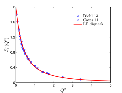
(a) (b)

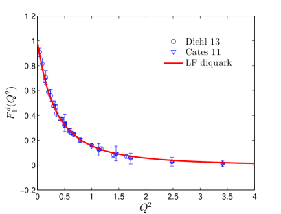
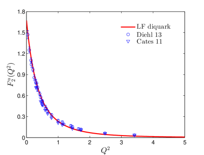
(c) (d)

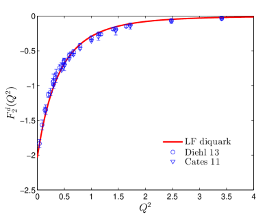
Figure 1: Flavour form factors fitting in the light-front diquark model. Data are taken from ref.Diehl13 ; Cates11 .

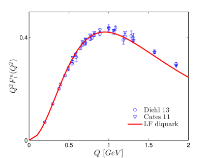
(a) (b)

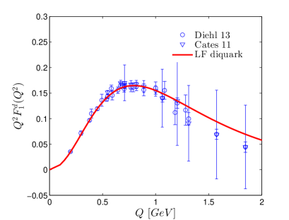
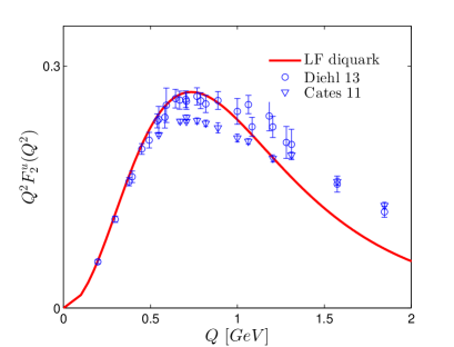
(c) (d)

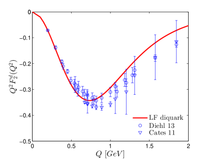
Figure 2: Dirac and pauli form factors multiplied by $Q^{2}$ for $u$ and $d$ quarks and compared with the dataDiehl13 ; Cates11 .

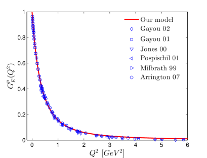
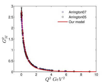
(a) (b)
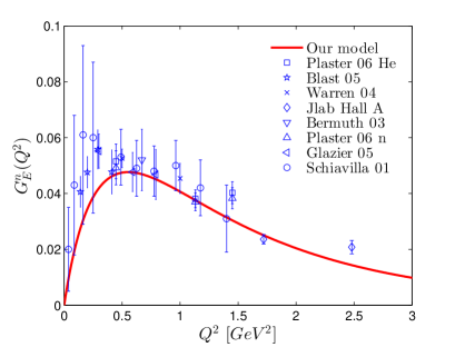
(c) (d)

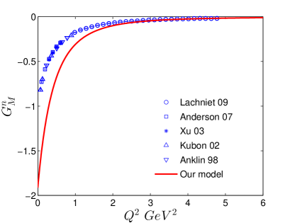
Figure 3: Sachs form factors $G^{p(n)}_{E}(Q^{2})$ and $G^{p(n)}_{M}(Q^{2})$ for proton(a,c) and neutron(b,d) respectively. The data are taken from ref.Gayou02 ; Gayou01 ; Jones00 ; Posp01 ; Milb99 ; Arri07 for $G^{p}_{E}(Q^{2})$, ref.Blast05 ; Warr04 ; JlabHA ; Berm03 ; Plas06 ; Glaz05 ; Schi01 for $G^{n}_{E}(Q^{2})$, ref.Arri07 ; Arri05 for $G^{p}_{M}(Q^{2})$ and ref.Lach09 ; Ande07 ; Xu03 ; Kubo02 ; Ankl98 for $G^{n}_{M}(Q^{2})$.

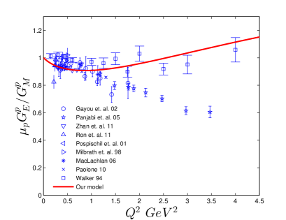
(a) (b)

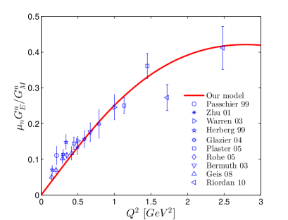
Figure 4: Ratio of Sachs form factor $R^{i}=\mu_{i}G^{i}_{E}/G^{i}_{M}$ for proton Gayou02 ; Posp01 ; Milb99 ; Punj05 ; Ron11 ; Walk94 ; Zhan11 ; Paol10 ; MacL06 and neutron Pass99 ; Zhu01 ; Warr04 ; Herb99 ; Glaz05 ; Plas06 ; Berm03 ; Blast05 ; Rior10 .

We find value of the parameters $a_{i}$ and $b_{i}$ by fitting Dirac and Pauli form factors data taken form Ref.Cates11 ; Diehl13 . Fig.1 shows the form factor fittings in our model.

$\nu$	$a_{1}^{\nu}$	$b_{1}^{\nu}$	$a_{2}^{\nu}$	$b_{2}^{\nu}$	$\delta^{\nu}$
$u$	$0.280\pm 0.001~{}$	$0.1716\pm 0.0051$	$0.84\pm 0.02$	$0.2284\pm 0.0035$	1.0
$d$	$0.5850\pm 0.0003$	$0.7000\pm 0.0002$	$0.9434^{+0.0017}_{-0.0013}$	$0.64^{+0.0082}_{-0.0022}$	1.0

Table 1: The fitted parameters for $u$ and $d$ quarks.

The normalization conditions are defined as

$$\int_{0}^{1}dxf^{(u)}_{1}(x) = F^{(u)}_{1}(Q^{2}=0)=n_{u},$$ (27)

$$\int_{0}^{1}dxE^{(u)}_{1}(x,0) = F^{(u)}_{2}(Q^{2}=0)=\kappa_{u},$$ (28)

$$\int_{0}^{1}dxf^{(d)}_{1}(x) = F^{(d)}_{1}(Q^{2}=0)=n_{d},$$ (29)

$$\int_{0}^{1}dxE^{(d)}_{1}(x,0) = F^{(d)}_{2}(Q^{2}=0)=\kappa_{d}.$$ (30)

Where $f_{1}^{\nu}(x)$ is the unpolarized PDF and $E^{(\nu)}(x,Q^{2})$ is the helicity flip GPD corresponding to the valence quark of flavour $\nu=u,d$ and according to the quark counting rules $n_{u}=2$ and $n_{d}=1$ for proton. From isospin symmetry, the anomalous magnetic moments for $u$ and $d$ quarks are $\kappa_{u}=1.673$ and $\kappa_{d}=-2.033$ respectively. The coefficients $C^{2}_{i}$ are then determined as

$$C^{2}_{S} = 1.3872,$$

$$C^{2}_{V} = 0.6128,$$ (31)

$$C^{2}_{VV} = 1.$$

The flavour decomposition of any distribution function follows the Eq.(10,11) with the $C^{2}_{i}$ given above in Eq.(31).

The normalized constants $N^{2}_{i}$ are found considering the following normalizations Bacc08

$$\int dxf^{(S)}_{1}(x)=F^{(S)}_{1}(0)=1,~{}\int dxf^{(V)}_{1}(x)=F^{(V)}_{1}(0)=1,~{}\int dxf^{(VV)}_{1}(x)=F^{(VV)}_{1}(0)=1;$$

and the values are $N_{S}=2.0191,~{}N_{0}^{(u)}=3.2050,~{}N_{0}^{(d)}=5.9423,~{}N_{1}^{(u)}=0.9895,~{}N_{1}^{(d)}=1.1616.$ To demonstrate the accuracy of the model, in Fig.2, the flavor form factors multiplied with $Q^{2}$ are compared with the available data. Even at large $Q^{2}$, the model predictions are within error bars of the experimental data.

The Sachs form factors for nucleons $(i=p,n)$ are defined as

$$G^{i}_{E}(Q^{2})=F^{i}_{1}(Q^{2})-\frac{Q^{2}}{4M^{2}_{i}}F^{i}_{2}(Q^{2}),$$ (32)

$$G^{i}_{M}(Q^{2})=F^{i}_{1}(Q^{2})+F^{i}_{2}(Q^{2}).$$ (33)

In Fig.3, the Sachs form factors $G_{E}$ and $G_{M}$ for proton and neutron in this model are shown to have excellent agreement with the experimental data, except for $G^{n}_{M}$. The ratio $R^{i}=\mu_{i}G^{i}_{E}/G^{i}_{M}$ for proton and neutron are also shown in Fig.4. They agree with the experimental data quite well. We also calculate the electromagnetic radii of nucleons from

$$\langle r^{2}_{E}\rangle^{i}=-6\frac{dG^{i}_{E}(q^{2})}{dQ^{2}}\bigg{|}_{Q^{2}=0},$$ (34)

$$\langle r^{2}_{M}\rangle^{i}=-\frac{6}{G^{i}_{M}(0)}\frac{dG^{i}_{M}(q^{2})}{dQ^{2}}\bigg{|}_{Q^{2}=0}$$ (35)

in this model. The radii are given in Table.2 show quit well agreement with measured data.

Quantity	Our  result	Measured Data Ber12
$r^{p}_{E}~{}(fm)$	$0.830\pm 0.025$	$0.877\pm 0.005$
$r^{p}_{M}~{}(fm)$	$0.779\pm 0.007$	$0.777\pm 0.016$
$\langle r^{2}_{E}\rangle^{n}~{}(fm^{2})$	$-0.064\pm 0.018$	$-0.1161\pm 0.0022$
$r^{n}_{M}~{}(fm)$	$0.758\pm 0.005$	$0.862^{+0.009}_{-0.008}$

Table 2: Electromagnetic radii of nucleon in this model compared with measured dataBer12

.

IV Unpolarized PDF evolution

The parton distribution function is defined as

$$\Phi^{\Gamma(\nu)}(x)=\frac{1}{2}\int\frac{dz^{-}}{2(2\pi)}e^{ip^{+}z^{-}/2}\langle P;S|\bar{\psi}^{(\nu)}(0)\Gamma\psi^{(\nu)}(z^{-})|P;S\rangle\bigg{|}_{z^{+}=z_{T}=0}.$$ (36)

which depends only on the light-cone momentum fraction $x=p^{+}/P^{+}$. Where the proton state $|P;S\rangle$, having spin $S$, is given in Eq.(1). For different Dirac structures we get different PDFs, e.g., for $\Gamma=\gamma^{+},\gamma^{+}\gamma^{5},i\sigma^{j+}\gamma^{5}$ we have the unpolarized PDF $f_{1}(x)$, helicity distribution $g_{1}(x)$ and transversity distribution $h_{1}(x)$ respectively.

The leading order QCD evolution of the unpolarized PDF is given as Bron08

$$\int^{1}_{0}dxx^{n}f_{1}(x,\mu)=\bigg{(}\frac{\alpha_{s}(\mu)}{\alpha_{s}(\mu_{0})}\bigg{)}^{\gamma^{(0)}_{n}/2\beta_{0}}\int^{1}_{0}dxx^{n}f_{1}(x,\mu_{0}).$$ (37)

Where the anomalous dimension is given as

$$\gamma^{(0)}_{n}=-2C_{F}\bigg{(}3+\frac{2}{(n+1)(n+2)}-4\sum_{k=1}^{n+1}\frac{1}{k}\bigg{)}$$ (38)

with $C_{F}=4/3$ and $\beta_{0}=9$. The strong coupling constant, at the leading order, is given as

$$\alpha_{s}(\mu)=\frac{4\pi}{\beta_{0}\ln(\mu^{2}/\Lambda^{2}_{QCD})}$$ (39)

with $\Lambda_{QCD}=0.226~{}GeV$. In Bron08 , for pion PDF evolution, the initial scale in leading order evolution was found to be $\mu_{0}=0.313$ GeV. For proton, we use the same initial scale.

The LFWFs are independent of the hard evolution scale $\mu$. Generally, the models of LFWFs are defined at the lowest scaleBacc08 and then DGLAP equation determines the PDF scale evolution. Thus, in the LFWF overlap representation, the unpolarised PDFs in the light-front diquark model at the initial scale $\mu_{0}$ are obtained as
for scalar diquark:

$$f^{(S)}_{1}(x) = \int d^{2}{\bf p}_{\perp}\frac{1}{16\pi^{3}}\bigg{[}|\psi^{+(u)}_{+}(x,{\bf p}_{\perp})|^{2}+|\psi^{+(u)}_{-}(x,{\bf p}_{\perp})|^{2}\bigg{]},$$ (40)

$$= N^{2}_{S}\bigg{[}\frac{1}{\delta^{u}}x^{2a_{1}^{u}}(1-x)^{2b_{1}^{u}+1}$$

$$~{}~{}~{}~{}~{}~{}~{}~{}~{}~{}~{}+x^{2a_{2}^{u}-2}(1-x)^{2b_{2}^{u}+3}\frac{\kappa^{2}}{(\delta^{u})^{2}M^{2}\ln(1/x)}\bigg{]},$$

for vector diquark:

$$f^{(A)}_{1}(x) = \int d^{2}{\bf p}_{\perp}\frac{1}{16\pi^{3}}\bigg{[}|\psi^{+(\nu)}_{++}(x,{\bf p}_{\perp})|^{2}+|\psi^{+(\nu)}_{-+}(x,{\bf p}_{\perp})|^{2}$$ (41)

$$~{}~{}~{}~{}~{}~{}~{}+|\psi^{+(\nu)}_{+0}(x,{\bf p}_{\perp})|^{2}+|\psi^{+(\nu)}_{-0}(x,{\bf p}_{\perp})|^{2}\bigg{]}$$

$$= \bigg{(}\frac{1}{3}N^{(\nu)2}_{0}+\frac{2}{3}N^{(\nu)2}_{1}\bigg{)}$$

$$\times\bigg{[}\frac{1}{\delta^{\nu}}x^{2a_{1}^{\nu}}(1-x)^{2b_{1}^{\nu}+1}+x^{2a_{2}^{\nu}-2}(1-x)^{2b_{2}^{\nu}+3}\frac{\kappa^{2}}{(\delta^{\nu})^{2}M^{2}\ln(1/x)}\bigg{]}.$$

Where $A$ represents the isoscalar-vector($V$) diquark corresponding to $u$ quark and isovector-vector($VV$) diquark corresponding to $d$ quark.

We simulate the scale evolution of the PDF by making the parameters in the PDF scale dependent where the values of the parameters at $\mu_{0}$ are the same as in the LFWFs. Thus, at a scale $\mu$, we parameterize the expressions for the PDFs as

$$f^{(S)}_{1}(x,\mu) = N^{2}_{S}(\mu)\bigg{[}\frac{1}{\delta^{u}(\mu)}x^{2a_{1}^{u}(\mu)}(1-x)^{2b_{1}^{u}(\mu)+1}$$ (42)

$$~{}~{}~{}~{}~{}~{}~{}~{}~{}~{}~{}+x^{2a_{2}^{u}(\mu)-2}(1-x)^{2b_{2}^{u}(\mu)+3}\frac{\kappa^{2}}{(\delta^{u}(\mu))^{2}M^{2}\ln(1/x)}\bigg{]},$$

$$f^{(A)}_{1}(x,\mu) = \bigg{(}\frac{1}{3}N^{(\nu)2}_{0}(\mu)+\frac{2}{3}N^{(\nu)2}_{1}(\mu)\bigg{)}$$ (43)

$$\!\!\!\times\bigg{[}\frac{1}{\delta^{\nu}(\mu)}x^{2a_{1}^{\nu}(\mu)}(1-x)^{2b_{1}^{\nu}(\mu)+1}+x^{2a_{2}^{\nu}(\mu)-2}(1-x)^{2b_{2}^{\nu}(\mu)+3}\frac{\kappa^{2}}{(\delta^{\nu}(\mu))^{2}M^{2}\ln(1/x)}\bigg{]}.$$

The assumption is that, not only at every scale there exists a set of parameters to reproduce the desired PDFs but we can also define an evolution formula for each of these parameters consistent with PDF evolution starting from the initial scale $\mu_{0}$.

The flavour decomposed PDFs are given as, from Eq.(10,11)

$$f^{u}_{1}(x,\mu) = C_{S}^{2}f^{(S)}_{1}(x,\mu)+C_{V}^{2}f^{(V)}_{1}(x,\mu),$$ (44)

$$f^{d}_{1}(x,\mu) = C_{VV}^{2}f^{(VV)}_{1}(x,\mu).$$ (45)

(a) (b)

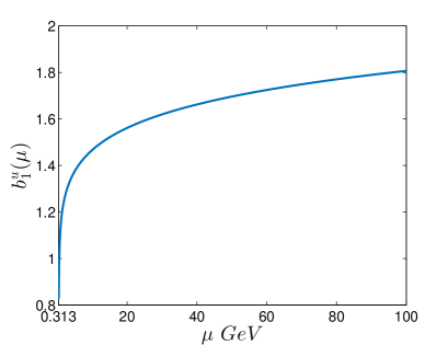
(c) (d)

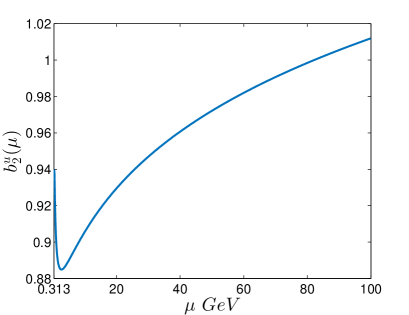
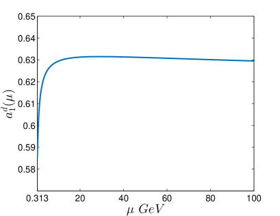
(a) (b)

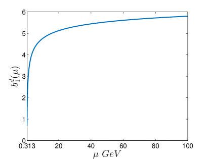
(c) (d)

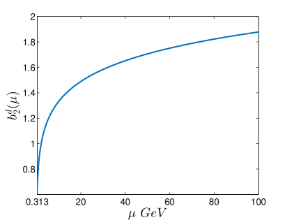
Figure 5: Scale evolution of the parameters [Eq.(47),(48)].

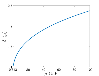
(a) (b)

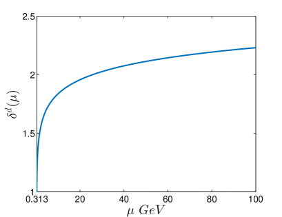
Figure 6: Variation of $\delta^{\nu}$ with $\mu$ for $u$ and $d$ quark, see Eq.49

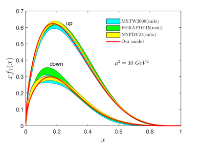
(a) (b)

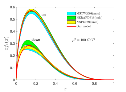
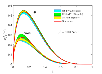
(c) (d)

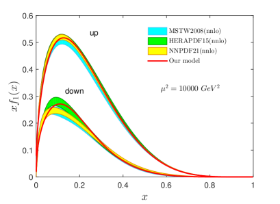
Figure 7: Evolution of unpolarized PDF in this model at $\mu^{2}=10,100,1000$ and $10000$ GeV² for both $u$ and $d$ quarks. Our model predictions are compared with NNPDF21(NNLO)NNPDF , HERAPDF15(NNLO)HERAPDF and MSTW2008(NNLO)MSTW results.

The PDF $f_{1}^{\nu}(x,\mu)$ at a scale $\mu$ can be written in our model as

$$f^{\nu}_{1}(x,\mu) = N^{(\nu)}\bigg{[}\frac{1}{\delta^{\nu}(\mu)}x^{2a_{1}^{\nu}(\mu)}(1-x)^{2b_{1}^{\nu}(\mu)+1}+x^{2a_{2}^{\nu}(\mu)-2}(1-x)^{2b_{2}^{\nu}(\mu)+3}\frac{\kappa^{2}}{(\delta^{\nu}(\mu))^{2}M^{2}\ln(1/x)}\bigg{]}.$$ (46)

The evolution of the parameters should be such that the PDF satisfies the master evolution equation, Eq.(37). The overall constants $N^{(u)}=(C_{S}^{2}N_{s}^{2}+C^{2}_{V}(\frac{1}{3}N_{0}^{(u)2}+\frac{2}{3}N_{1}^{(u)2}))$ and $N^{(d)}=C^{2}_{VV}(\frac{1}{3}N_{0}^{(d)2}+\frac{2}{3}N_{1}^{(d)2})$ for $u$ and $d$ quarks respectively. To fit the PDF data from NNPDF21(nnlo)NNPDF , we find that the scale dependence of the parameters can be written as

$$a_{i}^{\nu}(\mu) = a_{i}^{\nu}(\mu_{0})+A^{\nu}_{i}(\mu),$$ (47)

$$b_{i}^{\nu}(\mu) = b_{i}^{\nu}(\mu_{0})-B^{\nu}_{i}(\mu)\frac{4C_{F}}{\beta_{0}}\ln\bigg{(}\frac{\alpha_{s}(\mu^{2})}{\alpha_{s}(\mu_{0}^{2})}\bigg{)},$$ (48)

$$\delta^{\nu}(\mu) = \exp\bigg{[}\delta^{\nu}_{1}\bigg{(}\ln(\mu^{2}/\mu_{0}^{2})\bigg{)}^{\delta^{\nu}_{2}}\bigg{]},$$ (49)

where the $a_{i}^{\nu}(\mu_{0})$ and $b_{i}^{\nu}(\mu_{0})$ are the parameters at $\mu=\mu_{0}$, given in Table.1. The parameter $\delta^{\nu}$ becomes unity at $\mu_{0}$ for both $u$ and $d$ quarks, as shown in Table.1. The scale dependent parts $A^{\nu}_{i}(\mu)$ and $B^{\nu}_{i}(\mu)$ evolve as

$$P^{\nu}_{i}(\mu) = \alpha^{\nu}_{P,i}~{}\mu^{2\beta^{\nu}_{P,i}}\bigg{[}\ln\bigg{(}\frac{\mu^{2}}{\mu_{0}^{2}}\bigg{)}\bigg{]}^{\gamma^{\nu}_{P,i}}\bigg{|}_{i=1,2},$$ (50)

where the subscript $P$ in the right hand side of the above equation stands for $P=A,B$ corresponding to $P^{\nu}_{i}(\mu)=A^{\nu}_{i}(\mu),B^{\nu}_{i}(\mu)$ respectively. Note that at $\mu=\mu_{0}$, $P^{\nu}_{i}(\mu_{0})=0$. The unpolarized PDF data are fitted for $\mu^{2}=1,6,16,30,65$ and $150~{}GeV^{2}$. The evolution parameters $\alpha_{P,i}^{\nu},~{}\beta_{P,i}^{\nu}$ and $\gamma_{P,i}^{\nu}$ are given in Table.3 and the $\delta^{\nu}_{i}$ are given in Table.4 with the least $\chi^{2}$ per degrees of freedom ($\chi^{2}/d.o.f$) corresponding to the PDF fit. The variation of $a_{i}^{\nu}(\mu)$, $b_{i}^{\nu}(\mu)$ and $\delta^{\nu}(\mu)$ with scale $\mu$ are shown in Fig.5 and in Fig.6 respectively. At the initial scale $\mu_{0}$, the strong coupling constant is large $\alpha_{s}(\mu_{0})/2\pi\sim 0.34$ and hence parameters evolve very fast for scales near the initial point. The rate of evolution decays down at higher scales where the coupling constant becomes small. In appendix A, we have listed the parameters at different scales and shown the fitting of the parameters at the above mentioned scales.

With the fitted parameters, we predict the unpolarized PDF at other scales and compare with NNPDF21(nnlo), HERAPDF15(nnlo) and MSTW2008(nnlo) results in Fig.7. Though to determine the evolution, we used up to $\mu^{2}=150$ GeV², Fig.7 shows that the model reproduces the PDF quite accurately at very high scales. According to Drell-Yan-West relationDY70 ; West70 , the quark distribution should go like $(1-x)^{p}$ as $x\to 1$ at large $\mu^{2}$ and the Dirac form factor $F_{1}(Q^{2})\sim 1/(Q^{2})^{(p+1)/2}$ as $Q^{2}\to\infty$ where $p$ is related to the number of valence quark. For, proton, the number of valence quark is three which also gives $p=3$. In our model, we observe that for $u$-quark the unpolarized PDF at large $\mu^{2}$ goes as $f_{1}^{u}\sim(1-x)^{3.35}$ as $x\to 1$ ( for $d$ quark $f_{1}^{d}\sim(1-x)^{3.09}$ ), and $F_{1}(Q^{2})\sim 1/(Q^{2})^{2.16}$ at large $Q^{2}$ which are consistent with Drell-Yan-West relation.

With these above PDF evolution parameters we can generate the scale evolution of the other distribution functions e.g. helicity distribution, transversity distribution, GPDs, TMDs etc. Now we show that the model can predict the helicity and transversity distributions at different scales.

$P_{i}^{\nu}(\mu)$	$\alpha_{i}^{\nu}$	$\beta_{i}^{\nu}$	$\gamma_{i}^{\nu}$	$\chi^{2}/d.o.f$
$A_{1}^{u}$	$-0.2058\pm 0.0187$	$-0.0318\pm 0.0209$	$0.405\pm 0.0937$	0.23
$B_{1}^{u}$	$1.551^{+0.034}_{-0.035}$	$0.0598\pm 0.0057$	$-0.4291\pm 0.0242$	0.02
$A_{2}^{u}$	$-0.1637\pm 0.0179$	$-0.0066\pm 0.0245$	$0.3758\pm 0.1111$	0.13
$B_{2}^{u}$	$1.426\pm 0.320$	$0.07780.0605$	$-0.7634^{+0.0241}_{-0.0251}$	0.07
$A_{1}^{d}$	$0.0061\pm 0.0098$	$-0.1535\pm 0.0257$	$1.391^{+0.246}_{-0.245}$	0.14
$B_{1}^{d}$	$2.072\pm 0.0193$	$-0.008^{+0.021}_{-0.022}$	$0.1728\pm 0.0972$	0.10
$A_{2}^{d}$	$-0.2493\pm 0.0456$	$-0.0116\pm 0.0408$	$0.1371\pm 0.1783$	0.29
$B_{2}^{d}$	$0.1399\pm 0.0737$	$0.0247\pm 0.1086$	$0.5733^{+0.0517}_{-0.0518}$	0.10

Table 3: PDF evolution parameters with 95% confidence bounds.

$\delta^{\nu}(\mu)$	$\delta_{1}^{\nu}$	$\delta_{2}^{\nu}$	$\chi^{2}/d.o.f$
$\delta^{u}$	$0.015\pm 0.008$	$1.667\pm 0.032$	1.16
$\delta^{d}$	$0.212\pm 0.0566$	$~{}0.5444\pm 0.1504$	0.81

Table 4: PDF evolution parameter $\delta^{\nu}_{1}$ and $\delta^{\nu}_{2}$ for $\nu=u,d$.

V Model predictions

V.1 Helicity distributions and axial charges

The polarized PDFs are evaluated as predictions of the model. In terms of the light front wave functions, the helicity distribution $g_{1}(x)$ in the quark-diquark model at the initial scale $\mu_{0}$ is defined as

$$g^{(S)}_{1}(x) = \int d^{2}{\bf p}_{\perp}\frac{1}{16\pi^{3}}\bigg{[}|\psi^{+(u)}_{+}(x,{\bf p}_{\perp})|^{2}-|\psi^{+(u)}_{-}(x,{\bf p}_{\perp})|^{2}\bigg{]},$$ (51)

$$g^{(A)}_{1}(x) = \int d^{2}{\bf p}_{\perp}\frac{1}{16\pi^{3}}\bigg{[}|\psi^{+(\nu)}_{++}(x,{\bf p}_{\perp})|^{2}-|\psi^{+(\nu)}_{-+}(x,{\bf p}_{\perp})|^{2}$$ (52)

$$~{}~{}~{}+|\psi^{+(\nu)}_{+0}(x,{\bf p}_{\perp})|^{2}-|\psi^{+(\nu)}_{-0}(x,{\bf p}_{\perp})|^{2}\bigg{]}.$$

for scalar and vector diquarks respectively. The scale evolutions of the polarized PDFs are simulated by the same scheme as the unpolarized PDF. The scale evolutions of the parameters are the same as given in Eqs.(47,48,49,50). Thus, the flavour dependent helicity distributions at a scale $\mu$ are given by

$$g^{u}_{1}(x,\mu) = \bigg{(}C_{S}^{2}N^{2}_{S}(\mu)+C^{2}_{V}\big{(}\frac{1}{3}N^{(u)2}_{0}(\mu)-\frac{2}{3}N^{(u)2}_{1}(\mu)\big{)}\bigg{)}\bigg{[}\frac{1}{\delta^{u}(\mu)}x^{2a_{1}^{u}(\mu)}(1-x)^{2b_{1}^{u}(\mu)+1}$$ (53)

$$~{}~{}~{}~{}-x^{2a_{2}^{u}(\mu)-2}(1-x)^{2b_{2}^{u}(\mu)+3}\frac{\kappa^{2}}{(\delta^{u}(\mu))^{2}M^{2}\ln(1/x)}\bigg{]},$$

$$g^{d}_{1}(x,\mu) = C^{2}_{VV}\bigg{(}\frac{1}{3}N^{(d)2}_{0}(\mu)-\frac{2}{3}N^{(d)2}_{1}(\mu)\bigg{)}\bigg{[}\frac{1}{\delta^{d}(\mu)}x^{2a_{1}^{d}(\mu)}(1-x)^{2b_{1}^{d}(\mu)+1}$$ (54)

$$~{}~{}~{}~{}~{}-x^{2a_{2}^{d}(\mu)-2}(1-x)^{2b_{2}^{d}(\mu)+3}\frac{\kappa^{2}}{(\delta^{d}(\mu))^{2}M^{2}\ln(1/x)}\bigg{]}.$$

Helicity PDF $g_{1}(x)$ are shown in Fig.8, at scale $\mu^{2}=1~{}GeV^{2}$, for $u$ and $d$ quarks. Following Bacc08 ; Hirai04 , we include a constant relative error of $10\%$ to $g^{u}_{1}$ and $25\%$ to $g^{d}_{1}$ in the data taken fromLSS02 . The errors in the model predictions are due to the uncertainties in the parameters as listed in Tab.5. The model predicts the helicity PDF for $u$ quark quite well.

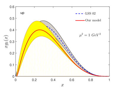
(a) (b)

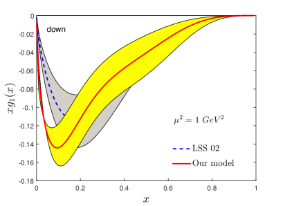
Figure 8: Helicity PDF at $\mu^{2}=1~{}GeV^{2}$ compared with ref.LSS02 . The error bands(yellow) in our model come from the errors in the evolution parameters given in Table.3.

	$g^{u}_{A}$	$g^{d}_{A}$	$g_{A}$	$g^{u(1)}_{A}$	$g^{d(1)}_{A}$	$g^{(1)}_{A}$
Our result	$0.71\pm 0.09$	$-0.54^{+0.19}_{-0.13}$	$1.25^{+0.28}_{-0.22}$	$0.18\pm 0.15$	$-0.052^{+0.003}_{-0.007}$	$0.23^{+0.15}_{-0.16}$
Measured Data	$0.82\pm 0.07$	$-0.45\pm 0.07$	$1.27\pm 0.14$	$0.19\pm 0.07$	$-0.06\pm 0.07$	$0.25\pm 0.14$

Table 5: Axial charge and second moment of helicity distribution at the scale $\mu^{2}=1~{}GeV^{2}$ and compared with LSS fit to experimental dataLead10 .

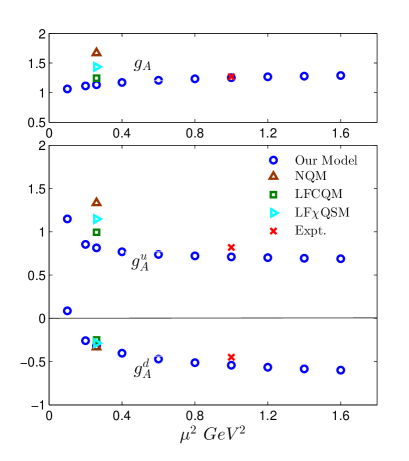
(a) (b)

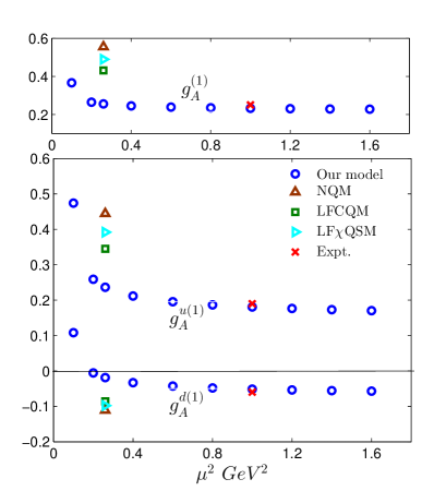
Figure 9: Scale evolution of axial charge in the range $\mu^{2}=0.1~{}to~{}1.6~{}GeV^{2}$ is shown in(a). We compare our result with other models e.g. NQM, LFCQM, LF$\chi$QSMLorce11 for $\mu^{2}=0.26$ GeV² and also with experimental value at $\mu^{2}=1.0~{}GeV^{2}$Lead10 . The second moment of helicity and a comparison with measured valueLead10 at $\mu^{2}=0.26,1.0~{}GeV^{2}$ are shown in (b). The top panels in the plots represent the total proton axial charge (a) and second moment of the total helicity distribution (b).

The axial charges which are obtained from the first moment of the helicity distributions are given in Table.5 and compared with the measured dataLead10 . The axial charge of proton is defined as

$$g_{A}=g_{A}^{u}-g_{A}^{d}.$$ (55)

The model prediction is in excellent agreement with the experimental data. The second moment of the helicity distributions are also presented in the table where $g_{A}^{\nu(1)}=\int_{0}^{1}dxxg_{1}^{\nu}(x)$ and $g_{A}^{(1)}$ is defined as

$$g_{A}^{(1)}=\int_{0}^{1}dxx(g_{1}^{u}(x)-g_{1}^{d}(x)).$$ (56)

In Fig.9(a), the scale evolution of the axial charges for $u$ and $d$ quarks are shown. The top panels in Fig.9(a) represents the axial charge of the proton, $g_{A}$. Results from other models and experimental data are shown in the same plot for comparison. Results from other models e.g., NQM, LFCQM, LF$\chi$QSMLorce11 at $\mu^{2}=0.26$ GeV² are in agreement with our model prediction and again our model predicts the experimental data at $\mu^{2}=1~{}\rm{GeV}^{2}$ (shown in red in Fig.9) quite well. In Fig.9(b), the scale evolution of the second moment of the helicity distributions for both $u$ and $d$ quarks are shown and compared with other model predictions and experimental data. The top panel in the plot represents $g_{A}^{(1)}$. Our model predictions show excellent agreement with the experimental data available at $\mu^{2}=1$ GeV².

V.2 Transversity distributions and tensor charges

(a) (b)

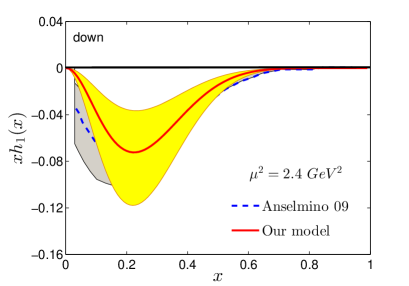
Figure 10: The transversity distribution at $\mu^{2}=2.4~{}GeV^{2}$ for $u$ quark(a) and $d$ quark(b). Our results are compared with Anselmino et. al.Anse09 .

The transversity distributions in this model reads as

$$h^{u}_{1}(x,\mu) = \bigg{(}C_{S}^{2}N^{2}_{S}(\mu)-C^{2}_{V}\frac{1}{3}N^{(u)2}_{0}(\mu)\bigg{)}\frac{1}{\delta^{u}}x^{2a^{u}_{1}(\mu)}(1-x)^{2b^{u}_{1}+1},$$ (57)

$$h^{d}_{1}(x,\mu) = -C^{2}_{VV}\frac{1}{3}N^{(d)2}_{0}(\mu)\frac{1}{\delta^{d}}x^{2a^{d}_{1}(\mu)}(1-x)^{2b^{d}_{1}+1}.$$ (58)

Transversity PDF $h_{1}(x)$ are shown in Fig.10, at scale $\mu^{2}=1~{}GeV^{2}$, for $u$ and $d$ quarks. The model predictions are shown to agree with the experimental dataAnse09 . The first moment of the transversity distribution gives the tensor charge $g_{T}$. The model again predicts the tensor charges quite accurately as shown in Table.6. For both $u$ and $d$ quarks, we have $\mid g_{T}^{\nu}\mid<\mid g_{A}^{\nu}\mid$. In Fig.11(a), we have compared our model predictions of tensor charge for both $u$ and $d$ quarks with other models along with the phenomenological fit of experimental dataAnse09 . Similar comparisons are studies by Anselmino et. al.Anse09 and WakamatsuWaka09 . Our predictions fall within the uncertainty bands of the phenomenological fits for both $u$ and $d$ quarks. The ratio of the two tensor charges $\mid{g_{T}^{d}}/{g_{T}^{u}}\mid$ is totally scale independent and a better quantity to compare with other models. Fig.11(b), shows the comparison of that ratio with other model predictions. Our model predicts $\mid{g_{T}^{d}}/{g_{T}^{u}}\mid=0.38$ which is very close to the phenomenological prediction.

	$g^{u}_{T}$	$g^{d}_{T}$	$g_{T}$
Our result	$0.37^{+0.06}_{-0.05}$	$-0.14^{+0.05}_{-0.06}$	$0.51^{+0.12}_{-0.11}$
Measured DataAnse07	$0.59^{+0.14}_{-0.13}$	$-0.20^{+0.05}_{-0.07}$	$0.79^{+0.19}_{-0.20}$

Table 6: Tensor charge at the scale $\mu^{2}=0.8~{}GeV^{2}$. Our results are compared with measured dataAnse07 .

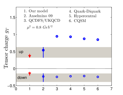
(a) (b)

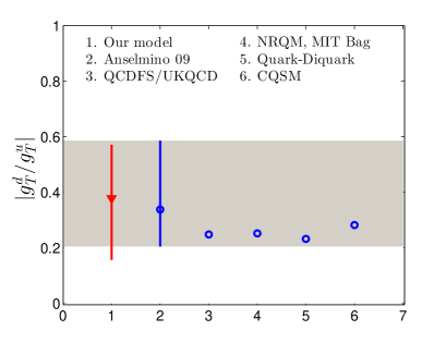
Figure 11: Comparisons of tensor charges $gT$ with the experimental data fit Anse09 and other model predictions Gock05 ; Cloet08 ; Pasq05 ; Waka07 are shown in (a), for $u$ and $d$ quarks. The shaded regions are the error band for $u$ and $d$ quarks in the experimental extraction of $g_{T}$Anse09 . Our results of tensor charges for both $u$ and $d$ quarks are shown in red. The ratio of the tensor charges $|g^{d}_{T}/g^{u}_{T}|$ is shown in (b). Our results are compared with other models e.g. Lattice QCDGock05 , MIT Bag model, Quark-Diquark modelCloet08 , CQSMWaka07 .

This model also satisfies the Soffer bound which at an arbitrary scale $\mu$ is defined as Soff95

$$|h^{\nu}_{1}(x,\mu)|\leq\frac{1}{2}\bigg{[}f^{\nu}_{1}(x,\mu)+g^{\nu}_{1}(x,\mu)\bigg{]}.$$ (59)

In Fig.12 we show the left (LHS) and right hand sides (RHS) of the the above equation multiplied by $x$ for both $\nu=u,d$ and at both low and high scales. According to Soffer bound, LHS should always lie below RHS which can be easily seen in Fig.12.

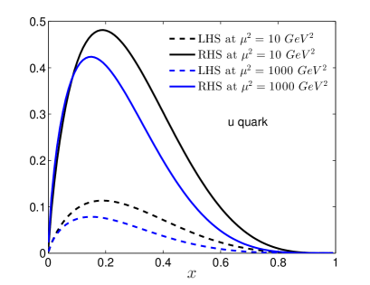
(a) (b)

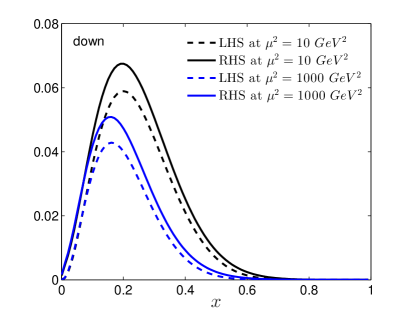
Figure 12: The Soffer bound at $\mu^{2}=10$ GeV², and $1000$ GeV² for (a) $u$ quark and (b) $d$ quark. Where the LHS and RHS stand for the left hand side and right hand side of Eq.(59) multiplied by $x$.

$\mu^{2}~{}(GeV^{2})$	$0.2$	0.6	1.0	7.0	10	20
$P_{q}$	0.60	0.48	0.45	0.38[0.55]	0.37	0.35

Table 7: Proton momentum fraction carried by valence quarks $P_{q}$ with the scale $\mu$. The value given within square bracket is the ZEUS result ZEUS03 at the scale $\mu^{2}=7~{}GeV^{2}$.

Proton momentum fraction carried by valence quarks can be estimated from the unpolarized PDFs at different scale $\mu$

$$P_{q}(\mu) = \int dxx[C_{S}^{2}f^{(s)}_{1}(x)+C_{V}^{2}f^{(V)}_{1}(x)+C_{VV}^{2}f^{(VV)}_{1}(x)],$$

$$= \int dxx[f^{(u)}_{1}(x,\mu)+f^{(d)}_{1}(x,\mu)].$$

The values of $P_{q}$ with the scale are shown in Table.7. The momentum carried by the valence quarks decreases as the value of $\mu^{2}$ increases.

VI Summary and conclusion

Light front Ads/QCD has predicted many interesting nucleon properties. Light front AdS/QCD predicts a particular form of wave function for a two body bound stateBT . In this paper, we have developed a quark-diquark model for proton where the light front wave functions are constructed from the AdS/QCD predictions. The model is consistent with the quark counting rule and Drell-Yan-West relation. The model has $SU(4)$ spin-flavor structure and includes the contributions from scalar($S=0$) and axial vector($S=1$) diquarks. The evolution of $f_{1}(x)$ is simulated by introducing scale dependence parameters in the PDF. The scale evolutions of the parameters are determined by satisfying the PDF evolution in the range $\mu^{2}=0.09GeV^{2}$ to $150GeV^{2}$. We have given the explicit scale evolution of each parameter in the model, so the distributions can be calculated at any arbitrary scale. Though PDF data up to $\mu^{2}=150$ GeV² are used to determine the scale evolution, we have shown that our model can accurately predict the PDF evolution up to a very high scale ($\mu^{2}=10^{4}~{}GeV^{2}$). The helicity and transversity PDFs are calculated as predictions of the model and are shown to satisfy Soffer bound and have good agreement with the available data. Our model reproduces the experimental values of axial and tensor charges quite well. It will be interesting to study the other proton properties like GPDs, TMDs, Wigner distributions and GTMDs etc and their scale evolutions in this model and compare with other model predictions.

Acknowledgements: DC thanks Stan Brodsky, Guy de Teramond for many insightful discussions. We also thank Chandan Mondal for many useful discussions.

Appendix A Parameter fitting for PDF evolution

Scale evolutions of $A_{i}^{\nu}$ and $B_{i}^{\nu}$ are parameterized by the parameters $\alpha_{i}^{\nu},~{}\beta_{i}^{\nu}$, and $\gamma_{i}^{\nu}$ and that of $\delta^{\nu}$ is parameterized by $\delta_{1}^{\nu}$ and $\delta_{2}^{\nu}$. $f_{1}(x,\mu)$ is given by Eq.(46) along with Eqs.(47,48,49) and Eq.(50). Here we list the parameters$A_{i}^{\nu},~{}B_{i}^{\nu}$ and $\delta^{\nu}$ fitted at different scales $\mu^{2}$ in Table 8 and Table 9. The last column in each table indicates the least $\chi^{2}$ error in the PDF estimation. Each $\chi^{2}/d.o.f$ has been evaluated from 100 data points for different $x~{}(0<x<1)$) i.e., for the five parameter fit, we have (100-5)=95 degrees of freedom. The fitting of the parameters at $\mu^{2}=1,6,16,30,65$ and $150$ GeV² are shown in Fig.13 and Fig.14. The data points are extracted from the PDF data. The error bars shown in the plots are the errors in the extracted values of the parameters due to the uncertainties in the PDF data.

$\mu^{2}~{}GeV^{2}$	$A_{1}^{u}$	$B_{1}^{u}$	$A_{2}^{u}$	$B_{2}^{u}$	$\delta^{u}$	$\chi^{2}/d.o.f$
1	$-0.29\pm 0.009$	$1.08\pm 0.009$	$-0.225\pm 0.008$	$0.75^{+0.047}_{-0.046}$	$1.087\pm 0.029$	1.41
6	$-0.343\pm 0.003$	$0.94\pm 0.007$	$-0.275\pm 0.004$	$0.55\pm 0.013$	$1.176\pm 0.027$	4.8
16	$-0.365\pm 0.001$	$0.91\pm 0.007$	$-0.295^{+0.003}_{-0.002}$	$0.52^{+0.013}_{-0.014}$	$1.234\pm 0.014$	1.8
30	$-0.375\pm 0.004$	$0.9^{+0.010}_{-0.012}$	$-0.31^{+0.003}_{-0.002}$	$0.49\pm 0.005$	$1.298\pm 0.018$	1.2
65	$-0.386\pm 0.002$	$0.89\pm 0.004$	$-0.323^{+0.002}_{-0.003}$	$0.47\pm 0.009$	$1.389\pm 0.025$	0.54
150	$-0.392\pm 0.001$	$0.89\pm 0.002$	$-0.334^{+0.0008}_{-0.001}$	$0.46\pm 0.008$	$1.515\pm 0.034$	0.29

Table 8: Fitting of the PDF $f_{1}(x)$ at various scales for $u$ quark.

$\mu^{2}~{}GeV^{2}$	$A_{1}^{d}$	$B_{1}^{d}$	$A_{2}^{d}$	$B_{2}^{d}$	$\delta^{d}$	$\chi^{2}/d.o.f$
1	$0.02\pm 0.007$	$2.4^{+0.029}_{-0.029}$	$-0.28^{+0.012}_{-0.017}$	$0.23^{+0.010}_{-0.011}$	$1.43\pm 0.085$	0.21
6	$0.03\pm 0.007$	$2.6^{+0.052}_{-0.051}$	$-0.29^{+0.006}_{-0.005}$	$0.32^{+0.024}_{-0.025}$	$1.54\pm 0.065$	0.38
16	$0.036\pm 0.005$	$2.68^{+0.017}_{-0.017}$	$-0.298\pm 0.001$	$0.38^{+0.009}_{-0.010}$	$1.65\pm 0.044$	0.40
30	$0.042\pm 0.001$	$2.74^{+0.018}_{-0.019}$	$-0.305\pm 0.002$	$0.42^{+0.008}_{-0.010}$	$1.75\pm 0.030$	0.49
65	$0.044\pm 0.002$	$2.78^{+0.020}_{-0.020}$	$-0.308\pm 0.001$	$0.46\pm 0.010$	$1.82\pm 0.048$	0.59
150	$0.045\pm 0.001$	$2.8^{+0.021}_{-0.020}$	$-0.309\pm 0.0008$	$0.49^{+0.016}_{-0.019}$	$1.86\pm 0.036$	0.77

Table 9: Fitting of the PDF $f_{1}(x)$ at various scales for $d$ quark. .

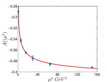
(a) (b)

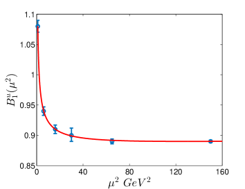
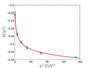
(c) (d)

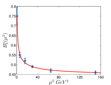
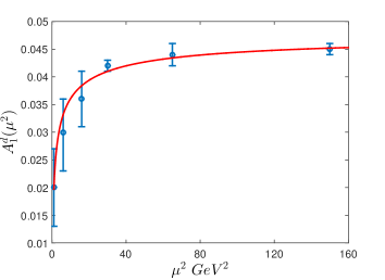
(e) (f)

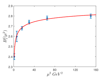
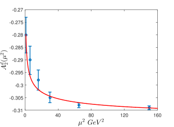
(g) (h)

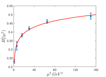
Figure 13: Using Eq.(50), the data of Table.8 are fitted by varying evolution parameters $\alpha^{\nu}_{P,i},\beta^{\nu}_{P,i}~{}and~{}\gamma^{\nu}_{P,i}$, for $u$ quark ($(a)-(d)$). Similar data fitting plots for $d$ quark(Table.9) are shown in $(e)-(h)$.

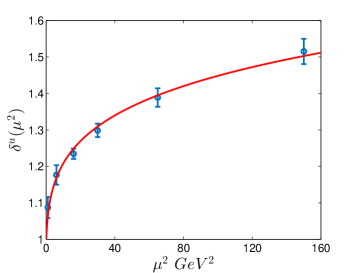
(a) (b)

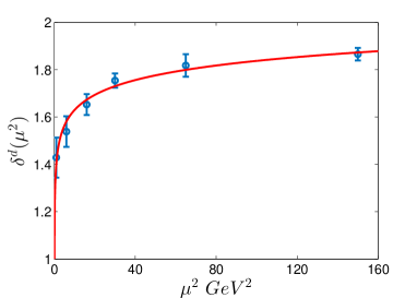
Figure 14: The data of Table.4 are fitted by varying evolution parameters $\delta^{\nu}_{1}$ and $\delta^{\nu}_{2}$, for (a) $u$ quark and (b) $d$ quark.

References

- (1) P. Kroll, M. Schurmann and W. Schweiger, Z. Phys. A 338 (1991) 339.; Int. J. Mod. Phys. A 6 (1991) 4107.
- (2) R. Jakob, P. Kroll, M. Schurmann and W. Schweiger, Z. Phys. A 347 (1993) 109 [hep-ph/9310227].
- (3) R. Jakob, P. J. Mulders and J. Rodrigues, Nucl. Phys. A 626 (1997) 937
- (4) A. Bacchetta, F. Conti and M. Radici, Phys. Rev. D 78 (2008) 074010.
- (5) S. J. Brodsky and G. F. de Teramond, Phys. Rev. D 77 (2008) 056007 [arXiv:0707.3859 [hep-ph]]; G. F. de Teramond and S. J. Brodsky, arXiv:1203.4025 [hep-ph].
- (6) T. Gutsche, V. E. Lyubovitskij, I. Schmidt and A. Vega, Phys. Rev. D 89, no. 5, 054033 (2014) Erratum: [Phys. Rev. D 92, no. 1, 019902 (2015)].
- (7) T. Gutsche, V. E. Lyubovitskij, I. Schmidt and A. Vega, Phys. Rev. D 91, 054028 (2015).
- (8) C. Mondal and D. Chakrabarti, Eur. Phys. J. C 75, no. 6, 261 (2015); D. Chakrabarti and C. Mondal, Phys. Rev. D 92, no. 7, 074012 (2015); D. Chakrabarti, C. Mondal and A. Mukherjee, Phys. Rev. D 91, no. 11, 114026 (2015); D. Chakrabarti, T. Maji, C. Mondal and A. Mukherjee, Eur. Phys. J. C 76, no. 7, 409 (2016).
- (9) A. Vega, I. Schmidt, T. Gutsche and V. E. Lyubovitskij, arXiv:1306.1597 [hep-ph].
- (10) T. Maji, C. Mondal, D. Chakrabarti and O. V. Teryaev, JHEP 1601 (2016) 165 [arXiv:1506.04560 [hep-ph]].
- (11) W. Broniowski, E. Ruiz Arriola and K. Golec-Biernat, Phys. Rev. D 77 (2008) 034023 [arXiv:0712.1012 [hep-ph]].
- (12) G. P. Lepage and S. J. Brodsky, Phys. Rev. D 22 (1980) 2157.
- (13) J. R. Ellis, D. S. Hwang and A. Kotzinian, Phys. Rev. D 80 (2009) 074033 [arXiv:0808.1567 [hep-ph]].
- (14) D. Chakrabarti and C. Mondal, Phys. Rev. D 88, no. 7, 073006 (2013); [arXiv:1307.5128 [hep-ph]]. Eur. Phys. J. C 73, 2671 (2013).
- (15) S. J. Brodsky and S. D. Drell, Phys. Rev. D 22 (1980) 2236.
- (16) G. D. Cates, C. W. de Jager, S. Riordan and B. Wojtsekhowski, Phys. Rev. Lett. 106 (2011) 252003 [arXiv:1103.1808 [nucl-ex]].
- (17) M. Diehl and P. Kroll, Eur. Phys. J. C 73 (2013) no.4, 2397 [arXiv:1302.4604 [hep-ph]].
- (18) J. Beringer et al. [Particle Data Group Collaboration], Phys. Rev. D 86 (2012) 010001.
- (19) O. Gayou et al., Phys. Rev. C 64 (2001) 038202.
- (20) M. K. Jones et al. [Jefferson Lab Hall A Collaboration], Phys. Rev. Lett. 84 (2000) 1398
- (21) J. Arrington, W. Melnitchouk and J. A. Tjon, Phys. Rev. C 76 (2007) 035205
- (22) J. Arrington, Phys. Rev. C 71 (2005) 015202 [hep-ph/0408261].
- (23) J. Lachniet et al. [CLAS Collaboration], Phys. Rev. Lett. 102 (2009) 192001 [arXiv:0811.1716 [nucl-ex]].
- (24) B. Anderson et al. [Jefferson Lab E95-001 Collaboration], Phys. Rev. C 75 (2007) 034003 [nucl-ex/0605006].
- (25) W. Xu et al. [Jefferson Lab E95-001 Collaboration], Phys. Rev. C 67 (2003) 012201 [nucl-ex/0208007].
- (26) G. Kubon et al., Phys. Lett. B 524 (2002) 26 [nucl-ex/0107016].
- (27) H. Anklin et al., Phys. Lett. B 428 (1998) 248.
- (28) O. Gayou et al. [Jefferson Lab Hall A Collaboration], Phys. Rev. Lett. 88 (2002) 092301 [nucl-ex/0111010].
- (29) T. Pospischil et al. [A1 Collaboration], Eur. Phys. J. A 12 (2001) 125.
- (30) B. D. Milbrath et al. [Bates FPP Collaboration], Phys. Rev. Lett. 80 (1998) 452 Erratum: [Phys. Rev. Lett. 82 (1999) 2221]
- (31) V. Punjabi et al., Phys. Rev. C 71 (2005) 055202 Erratum: [Phys. Rev. C 71 (2005) 069902] [nucl-ex/0501018].
- (32) G. Ron et al. [Jefferson Lab Hall A Collaboration], Phys. Rev. C 84 (2011) 055204 [arXiv:1103.5784 [nucl-ex]].
- (33) R. C. Walker et al., Phys. Rev. D 49 (1994) 5671.
- (34) X. Zhan et al., Phys. Lett. B 705 (2011) 59 [arXiv:1102.0318 [nucl-ex]].
- (35) G. MacLachlan et al., Nucl. Phys. A764 (2006) 261.
- (36) M. Paolone et al., Phys. Rev. Lett. 105 (2010) 072001 [arXiv:1002.2188 [nucl-ex]].
- (37) E. Geis et al. [BLAST Collaboration], Phys. Rev. Lett. 101 (2008) 042501 [arXiv:0803.3827 [nucl-ex]].
- (38) G. Warren et al. [Jefferson Lab E93-026 Collaboration], Phys. Rev. Lett. 92 (2004) 042301 [nucl-ex/0308021].
- (39) S. Riordan et al., Phys. Rev. Lett. 105 (2010) 262302 [arXiv:1008.1738 [nucl-ex]].
- (40) J. Bermuth et al., Phys. Lett. B 564 (2003) 199 [nucl-ex/0303015].
- (41) B. Plaster et al. [Jefferson Laboratory E93-038 Collaboration], Phys. Rev. C 73 (2006) 025205 [nucl-ex/0511025].
- (42) D. I. Glazier et al., Eur. Phys. J. A 24 (2005) 101 [nucl-ex/0410026].
- (43) R. Schiavilla and I. Sick, Phys. Rev. C 64 (2001) 041002 [nucl-ex/0107004].
- (44) I. Passchier et al., Phys. Rev. Lett. 82 (1999) 4988 [nucl-ex/9907012].
- (45) H. Zhu et al. [E93026 Collaboration], Phys. Rev. Lett. 87 (2001) 081801 [nucl-ex/0105001].
- (46) C. Herberg et al., Eur. Phys. J. A 5 (1999) 131.
- (47) S. Riordan et al., Phys. Rev. Lett. 105 (2010) 262302 [arXiv:1008.1738 [nucl-ex]].
- (48) M. Hirai et al. [Asymmetry Analysis Collaboration], Phys. Rev. D 69 (2004) 054021 [hep-ph/0312112].
- (49) L. Del Debbio et al. [NNPDF Collaboration], JHEP 0703 (2007) 039 [hep-ph/0701127].
- (50) F. D. Aaron et al. [H1 and ZEUS Collaborations], JHEP 1001 (2010) 109 [arXiv:0911.0884 [hep-ex]].
- (51) A. D. Martin, W. J. Stirling, R. S. Thorne and G. Watt, Eur. Phys. J. C 63 (2009) 189, [arXiv:0901.0002 [hep-ph]].
- (52) S. D. Drell and T. M. Yan, Phys. Rev. Lett. 24 (1970) 181.
- (53) G. B. West, Phys. Rev. Lett. 24 (1970) 1206.
- (54) E. Leader and D. B. Stamenov, Phys. Rev. D 67 (2003) 037503 [hep-ph/0211083].
- (55) C. Lorce, Phys. Lett. B 735 (2014) 344. [arXiv:1401.7784 [hep-ph]].
- (56) C. Lorce, B. Pasquini and M. Vanderhaeghen, JHEP 1105 (2011) 041 [arXiv:1102.4704 [hep-ph]].
- (57) E. Leader, A. V. Sidorov and D. B. Stamenov, Phys. Rev. D 82 (2010) 114018
- (58) M. Anselmino, M. Boglione, U. D’Alesio, A. Kotzinian, F. Murgia, A. Prokudin and C. Turk, Phys. Rev. D 75 (2007) 054032 [hep-ph/0701006].
- (59) M. Anselmino, M. Boglione, U. D’Alesio, A. Kotzinian, F. Murgia, A. Prokudin and S. Melis, Nucl. Phys. Proc. Suppl. 191 (2009) 98 [arXiv:0812.4366 [hep-ph]].
- (60) M. Gockeler et al. [QCDSF and UKQCD Collaborations], Phys. Lett. B 627 (2005) 113 [hep-lat/0507001].
- (61) I. C. Cloet, W. Bentz and A. W. Thomas, Phys. Lett. B 659 (2008) 214 [arXiv:0708.3246 [hep-ph]].
- (62) B. Pasquini, M. Pincetti and S. Boffi, Phys. Rev. D 72 (2005) 094029 [hep-ph/0510376].
- (63) M. Wakamatsu, Phys. Lett. B 653 (2007) 398 [arXiv:0705.2917 [hep-ph]].
- (64) M. Wakamatsu, Phys. Rev. D 79 (2009) 014033 [arXiv:0811.4196 [hep-ph]].
- (65) J. Soffer, Phys. Rev. Lett. 74 (1995) 1292 [hep-ph/9409254].
- (66) S. Chekanov et al. [ZEUS Collaboration], Phys. Rev. D 67 (2003) 012007 [hep-ex/0208023].