Magnetic excitation spectra of strongly correlated quasi-one dimensional systems: Heisenberg versus Hubbard-like behavior

Abstract

We study the effects of charge degrees of freedom on the spin excitation dynamics in quasi-one dimensional magnetic materials. Using the density matrix renormalization group method, we calculate the dynamical spin structure factor of the Hubbard model at half electronic filling on a chain and on a ladder geometry, and compare the results with those obtained using the Heisenberg model, where charge degrees of freedom are considered frozen. For both chains and two-leg ladders, we find that the Hubbard model spectrum qualitatively resembles the Heisenberg spectrum – with low-energy peaks resembling spinonic excitations – already at intermediate on-site repulsion as small as $U/t\sim 2-3$, although ratios of peak intensities at different momenta continue evolving with increasing $U/t$ converging only slowly to the Heisenberg limit. We discuss the implications of these results for neutron scattering experiments and we propose criteria to establish the values of $U/t$ of quasi-one dimensional systems described by one-orbital Hubbard models from experimental information.

I Introduction

In recent years, we have witnessed a considerable improvement in the momentum and frequency resolution of inelastic neutron scattering techniques, which have been shown to be powerful tools to analyze the magnetic excitation dynamics in low dimensional strongly correlated materials. A typical example of the accurate agreement between theory and experiment is given by the dynamical spin structure factor of the one-dimensional spin 1/2 Heisenberg quantum magnet $\textrm{KCuF}_{3}$.Lake et al. (2013)

Strongly correlated materials are often described in terms of model Hamiltonians where only spin degrees of freedom are taken into account—typically the Heisenberg Hamiltonian, which represents the main paradigm for quantum magnetism. This is due to the presence of strong electronic correlations, which energetically forbid the possibility of double occupation of the outer shell orbitals. In these systems, charge degrees of freedom are considered frozen (or gapped), and the low-energy magnetic excitations can be understood in terms of the sole spin degrees of freedom.

The idea of using a Heisenberg Hamiltonian as a “phenomenological” model, even in cases when it is known that it is not fully applicable, is not new. For instance, the description of the spin waves in iron in the low-energy regime has been discussed in terms of the Heisenberg modelCollins et al. (1969); Perring et al. (1991) since the early days of neutron scattering. Even though this system is clearly itinerant, the Heisenberg model works because it captures the essential features of the dispersion relation in this low-energy regime. However, it was known that this model could not explain the higher energy features of the magnetic excitation spectrum, features requiring a more realistic treatment that accounts for the itinerant nature of electrons in iron.

One- and quasi-one- dimensional (1D) Mott insulators, such as spin chains and ladders, provide an exciting playground for the study of strongly correlated quantum states of matter. In 1D, one can observe quasi-long-range order states, known as Tomonaga-Luttinger liquids,Giamarchi (2004) or phases where correlations between magnetic excitations are short range as in the case of Haldane spin-1 chains.Haldane (1983) In ladders, quantum spin-liquid phases have properties quite different from those of any conventional ferro- or antiferromagnet.Dagotto et al. (1992) In particular, for even number of legs—including the important case of two-leg ladders—the decay of correlations is exponential due to the presence of the spin gap.White et al. (1994); Dagotto and Rice (1996); Maekawa (1996); Tranquada et al. (2004) The existence of this spin gap has been confirmed experimentally in the copper oxide SrCu₂O₃.Azuma et al. (1994) Spin ladders have applications ranging from high-temperature superconductorsDai et al. (2012); Dagotto (2013); Takahashi et al. (2015); Patel et al. (2016) to ultracold atoms.Duan et al. (2003); García-Ripoll et al. (2004) Recently, unusual and intriguing physical phenomena were observed in spin systems, such as the Bose-Einstein condensation of magnons,Zapf et al. (2014) the fractionalization of spin excitations,Thielemann et al. (2009); Bouillot et al. (2011) spinon attraction,Schmidiger et al. (2012) and unusual disorder effects.Yu et al. (2012) Excellent agreement between theory and experiment has been achieved without considering charge dynamics effects in the study of the magnetic excitation spectrum, as the example of KCuF₃ shows.Lake et al. (2013) Yet the effects of the charge degree of freedom cannot always be neglected, as will be shown in this paper.

An example of the need to consider charge is provided by the two-dimensional Mott insulating cuprate La₂CuO₄, where the experimentally observed magnetic dispersion departs noticeably from the pure Heisenberg form.Coldea et al. (2001) Starting from the Hubbard model, a perturbation theory in the electronic hopping term has shown that ring exchange terms appear beyond second order, and they are needed to understand the unusual magnetic dispersion and thus restore the agreement between theory and experiment. This is a direct manifestation that electronic itinerancy or charge dynamics effects are important to understand the magnetic excitation spectra of strongly correlated materials.

A recent theoretical studyBhaseen et al. (2005) of the dynamical spin structure factor in the 1D Hubbard model Essler et al. (2003) has shown that there are significant charge dynamics effects (a transfer of spectral weight) due to the coupling of the spin excitations to charge fluctuations at low and intermediate values of the Hubbard interaction. In this regime, the spin structure factor of the Hubbard model differs from the spectrum of the Heisenberg model, that is, the strong-coupling limit $U/t$ of the half-filled Hubbard model, where charge dynamics is suppressed and electrons are completely localized. These results have been confirmed in a density matrix renormalization group or DMRGWhite (1992, 1993) study in ref. Benthien and Jeckelmann, 2007.

Motivated by the mentioned work, this paper studies the dynamical spin structure factor of the Heisenberg and the Hubbard model at half-filling, not only for the case of chains, but also for two leg ladders. The aim of this paper is to provide a quantitative criterion to determine when a Hubbard model description of the material under consideration should be preferred to the simpler Heisenberg description.

The paper is organized as follows. Section II provides an introduction to the dynamical spin structure factor and explains how it is computed with DMRG. Section III presents calculations of the dynamical spin structure factor of the Heisenberg, and of the Hubbard model on a chain. Section IV extends the comparison between the two models studied above in the case of a ladder geometry. The last section presents a summary and conclusions.

II Dynamical Spin Structure Factor

In this publication we compute spectral functions directly in frequency. We follow closely the correction-vector method proposed by Kuhner and White in ref. Kühner and White, 1999, and calculate

$$S_{i,c}(\omega)=\langle\Psi_{0}|S^{z}_{i}\frac{1}{\omega-H+E_{g}+i\eta}S^{z}_{c}|\Psi_{0}\rangle,$$ (1)

at each frequency $\omega$ for all sites of the lattice, where $E_{g}$ is the ground state energy of the time-independent Hamiltonian $H$. We consider quasi-one dimensional systems with two possible geometries: chains and two-leg ladders. In the case of a chain, the index $i$ is equal to the only coordinate of the corresponding site of the chain. In the case of a two-leg ladder, the index $i\equiv(i_{x},i_{y})$ corresponds to the two coordinates of the site on the ladder; $i_{y}=0$ ($i_{y}=1$) for the lower (upper) leg of the ladder. The center site $c=L/2-1$ in the case of a chain, and $c\equiv(L/4-1,0)$ in the case of the $L/2\times 2$ ladder. The chain geometry has $L$ sites, numbered from $0$ to $L-1$; the ladder has also $L$ sites in total. The DMRG correction vector methodKühner and White (1999) will be used throughout. Within correction vector we use the Krylov decomposition instead of conjugate gradient. A computational advantageNocera and Alvarez (2016) of Krylov decomposition is that the main source of error is given by the Krylov method used for the calculation of the correction vector. Different frequencies can be computed in parallel, decreasing the CPU time needed for the computation of the entire spectrum. The constant $\eta$ has the dimension of an energy, and constitutes an external parameter for the DMRG simulations; $\eta$ controls the broadening of the spectral function peaks. The above quantity is finally transformed to momentum space as

$$S(k,\omega)=\sqrt{\frac{2}{L+1}}\sum_{j=0}^{L-1}\sin((j-c)k)S_{j,c}(\omega+i\eta),$$ (2)

where the quasi-momenta $k=\frac{\pi n}{L+1}$ with $n=1,..,L$ are appropriate for open boundary conditions. The DMRG implementation used throughout this paper has been discussed in ref. Nocera and Alvarez, 2016; technical details are in the supplemental material, which can be found at https://drive.google.com/open?id=0B4WrP8cGc5JHWXhkcG5wNzk5TDA.

III One dimensional Chains

III.1 Antiferromagnetic Heisenberg model

For a generic quasi-one dimensional geometry, the Hamiltonian of the antiferromagnetic Heisenberg model is given by

$$H_{Heis}=\sum_{i,j}J_{i,j}\vec{S}_{i}\cdot\vec{S}_{j},$$ (3)

with $\vec{S}=(S^{x},S^{y},S^{z})$. For a chain with open boundaries, $J_{i,j}=J$ if $i$ and $j$ are nearest neighbors, and $0$ otherwise. $J_{i,j}$ will be specialized for ladders in section IV.1.

The magnetic excitation spectrum of the antiferromagnetic Heisenberg chain has been studied thoroughly in the literature, using exact diagonalization,Lin (1990) DMRGHallberg (1995); Kühner and White (1999); Benthien and Jeckelmann (2007) and analytical approaches.Karbach et al. (1997); Müller et al. (1981) The ground state energy $E_{GS}=LJ(1/4-\ln 2)$, and the asymptotic behavior of the static correlation function isAffleck (1998)

$$\langle GS|\vec{S}_{n}\cdot\vec{S}_{0}|GS\rangle\propto(-1)^{n}\frac{[\ln(n)]^{1/2}}{n},$$ (4)

resulting in a weakly diverging static structure factor at $k\simeq\pi$

$$S(k)\propto|\ln|k-\pi||^{\frac{3}{2}}.$$ (5)

The Bethe ansatz shows that the manifold of the lowest excited states consists of a continuum delimited by a lower and an upper boundary, given by the des Cloiseaux-Pearson (dCP) dispersions. The majority of the spectral weight is concentrated in the lower boundary, $\omega^{l}(k)=(J\pi/2)\sin(k)$, which is gapless for $q=0$ and $q=\pi$, and repeats itself in the other half of the Brillouin zone. Its physical meaning can be explained as follows: a flip of a single spin in the antiferromagnetic chain creates a pair of spinons (block domain walls in the lattice) having opposite momentum. The spin flip terms in the Hamitonian (3) move the spinons by two lattice spacings, giving to the dCP dispersion twice the period. The upper boundary of the excitation manifold is given by $\omega^{u}(k)=J\pi|\sin(k/2)|$. The approximate expression

$$S(k,\omega)=\frac{A}{\sqrt{\omega^{2}-\omega^{l}(k)^{2}}}\theta(\omega-\omega^{l}(k))\theta(\omega^{u}(k)-\omega)$$ (6)

has been proposed by Muller et al. in ref. Müller et al., 1981 to describe all the features mentioned, where $A$ is a normalization constant, and $\theta$ is the standard step function. This ansatz describes very accurately the numerical results obtained with correction-vector DMRGNocera and Alvarez (2016) and time dependent DMRG.Lake et al. (2013) A very good agreement between theory (Bethe ansatz) and experiment has been obtained using a spin $1/2$ Heisenberg chain model description for the compound $\text{CuSO}_{4}\cdot 5\text{D}_{2}\text{O}$.Mourigal et al. (2013) In the supplemental material, which can be found at https://drive.google.com/open?id=0B4WrP8cGc5JHWXhkcG5wNzk5TDA, we have verified that the Krylov method compares well with the spectra obtained using a two-spinon exact calculation presented in ref. Karbach et al., 1997 for a Heisenberg model. The two spinon solution proposed in ref. Karbach et al., 1997 has a similar behavior to the dynamical spectrum of the Haldane-Shastry modelHaldane and Zirnbauer (1993), because the latter is in the same low-energy universality class of the standard Heisenberg model.

From the Bethe ansatz solution of the Heisenberg model, it follows that the $S(k,\omega)$ diverges as

$$S(k,\omega) \sim[\omega-\omega^{l}]^{-1/2}\sqrt{\ln[1/(\omega-\omega^{l})]}~{}\text{for}~{}k\neq\pi,$$ (7)

$$S(\pi,\omega) \sim\omega^{-1}\sqrt{\ln(1/\omega)},$$

as $\omega$ approaches the lower boundary $\omega^{l}(k)$ from above for any $k$ value. This divergence has its profound origin in the Luttinger liquid characteristics of the ground state, describes the instability of the model toward antiferromagnetic ordering, and is expected to still be present for the Hubbard model on a chain at finite $U$; see next section. For finite size systems, one usually cuts off the divergences at $\omega-\omega^{l}\simeq 1/L$, so that one has peaks of finite height

$$\text{max}[S(k,\omega)] \sim[L\ln(L)]^{1/2}~{}\text{for}~{}k\neq\pi,$$ (8)

$$\text{max}[S(\pi,\omega)] \sim L\ln(L)^{1/2}.$$

Experimentally, it is not always possible to collect inelastic neutron scattering data in the whole relevant range of $k$ and $\omega$, using a single instrument or a single configuration. This is because the measurements at low energies require higher energy resolution, and because of kinematical constraints of the neutron scattering geometry. In these cases much care need to be exercised to make direct comparisons between the calculated and measured $S(k,\omega)$ over the whole range of $k$ and $\omega$.

III.2 Hubbard model and Comparison to Heisenberg

This section reviews and studies the dynamical spin properties of the Hubbard model with Hamiltonian

$$H=-\sum\limits_{i,j,\sigma}t_{i,j}c^{\dagger}_{i,\sigma}c_{j,\sigma}+U\sum\limits_{i}n_{i,\uparrow}n_{i,\downarrow},$$ (9)

where $U\geq 0$ represents the onsite Coulomb repulsion. In the case of a chain with open boundaries, $t_{i,j}=t$ if $i$ and $j$ are nearest neighbours, and $0$ otherwise. $t_{i,j}$ will be specialized for ladders in section IV.2.

Figure 1 shows the dynamical spin structure factor $S(k,\omega)$ calculated with DMRG for a chain of length $L=64$ for different values of the Coulomb repulsion $U$. In this figure, the electronic hopping $t=1$ is assumed as unit of energy, and a broadening of the spectral peaks equal to $\eta=0.05$ is used.

At $U=0$, similarly to the case of the Heisenberg chain analyzed in the previous section, the excitation spectrum is enclosed between an upper boundary $\omega_{u}(k)=4t|\sin(k/2)|$ and a lower boundary $\omega_{l}(k)=2t|\sin(k)|$. The boundaries stem from the cosine-like non interacting band structure of the model. Panels (a-b) and (c-d) of fig. 2 contain cuts at $k=\pi$ and $k=\pi/2$ of the spectra shown in fig. 1, respectively. For $k=\pi$, as opposed to the Heisenberg case, the spectral weight is concentrated mostly at the upper boundary $\omega/(4t)\simeq 0.95\simeq\omega_{u}(0)$. Similarly, for $k=\pi/2$ the spectral weight is concentrated in the interval of frequencies $0.5<\omega/(4t)<0.8$ with a peak at $\omega/(4t)\simeq 0.65\simeq\omega_{u}(\pi/2)$.

When electron-electron interactions are turned on, the charge dynamics manifests itself on the magnetic excitation spectrum as a spectral weight redistribution to lower energies.Bhaseen et al. (2005) For $U=1.0$, the dashed (red) curve in fig. 2a representing the cut of the spectrum at $k=\pi$ shows two weak peaks: at $\omega/(4t)\simeq 0.9$ and at the lower energy of $\omega/(4t)\simeq 0.05$. A different behavior is observed for the cut at $k=\pi/2$ where the peak position is shifted to lower energies $\omega/(4t)\simeq 0.55$ with an asymmetric triangular shape.

For $U=2$, the renormalization of the spectral weight has already proceeded to lower frequencies and the high energy peak characteristic of the non interacting case at $k=\pi$ has almost disappeared: it is barely visible in our data at $\omega/(4t)\simeq 0.8$, as the short dashed (green) curve in fig. 2a shows. For $k=\pi/2$, the triangular shape spectral feature shows a peak at $\omega/(4t)\simeq 0.45$.

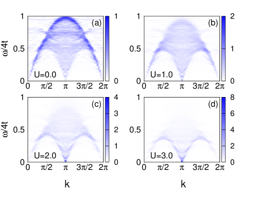
Figure 1: (Color online) $S(k,\omega)$ for a Hubbard model on a chain of $L=64$ sites at half-filling for different values of $U$, as indicated. The number of states kept for the DMRG is $m=1000$, $\eta/t=0.05$, while the number of sweeps is $4$.

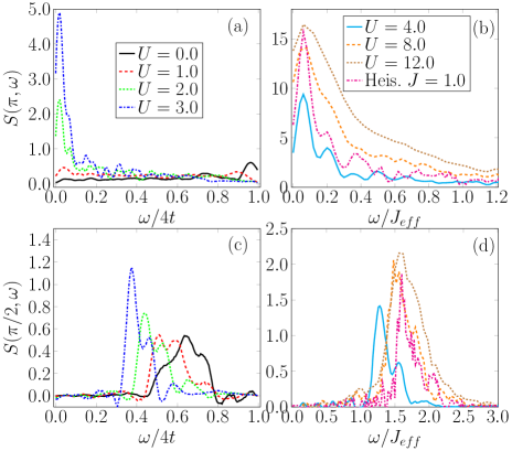
Figure 2: (Color online) Panel (a)-(c): cuts of fig. 1 as a function of $\omega/(4t)$. Panel (b)-(d): cuts of spectra obtained for larger values of $U$, together with the Heisenberg case cuts. In panels (b,d), on the x-axis we have plotted frequencies in units of $\omega/J_{\text{eff}}$, where $J_{\text{eff}}=4t^{2}/U$. Panels (c) and (d) show cuts of the spectrum at $k=\pi/2$. In panels (a) and (c), we have used $\Delta\omega/t=0.02$ and $\eta/t=0.05$. In panels (b) and (d), for $U=8$, we have $\Delta\omega/J_{\text{eff}}=0.04$ while for $U=12$ $\Delta\omega/J_{\text{eff}}=0.06$. $\eta/t=0.05$ for the Hubbard and $\eta/J=0.05$ for the Heisenberg curves.

As noticed in ref. Benthien and Jeckelmann, 2007, the spectral weight transfer to lower energies is quite fast as a function of $U$, and for $U=3$ most of the spectral weight is already concentrated very close to the lower boundary of the dCP dispersion of the Heisenberg model discussed in the previous section; notice the two very well defined dashed-dotted (blue) line spectral features in panels (a-b) of fig. 2. In particular, notice the similarity between the $U=3$ data and the results obtained from the Heisenberg model.Lake et al. (2013)

For larger values of $U$, shown in panels (b-d) of fig. 2, the spectral weight redistribution continues to approach the Heisenberg-like limit. As can be inferred from fig. 1, this redistribution happens for all $k$ values; we have shown them only for $k=\pi$ and $k=\pi/2$. The replicas of the main peak at larger frequencies in panel (c) of fig. 2 are artifacts due to finite size effects and the use of a tiny broadening $\eta=0.05$.

In these two panels, the cuts are plotted as a function of the quantity $\omega/J_{\text{eff}}$. It is well known that, in the case of half filling and large $U$, charge fluctuations are suppressed and the Hubbard model maps onto the antiferromagnetic Heisenberg chain with an effective exchange coupling constant $J_{\text{eff}}=4t^{2}/U$. The results compare very well with those obtained by Benthien and Jeckelmann in ref. Benthien and Jeckelmann, 2007, giving a well defined antiferromagnetic peak at $\pi$.

Panel (a) of fig. 3 shows the ratio of the peak maxima for $k=64\pi/65$ (closest to $\pi$ for an open chain)) and $k=31\pi/65$ (closest to $\pi/2$ for an open chain) as a function of $U$ for the Hubbard model. Panel (b) shows another ratio between the peak maxima for $k=56\pi/65$ (close to $6\pi/7$) and $k=22\pi/65$ (close to $\pi/3$) as a function of $U$. In both panels, for $U/t>2$, the ratios of the peaks maxima of the Hubbard model tend continuously to the Heisenberg model ratio. The shaded (red) region indicates the interval of values for the Heisenberg ratio compatible with our resolution in momentum space $\Delta k=2\pi/L$ (due to finite system size effects), the resolution in frequency $\Delta\omega\leq\eta$, and the extrinsic broadening $\eta$ of the spectral function peaks. The width of the shaded region has been estimated as follows. The extrinsic broadening $\eta$ and the system size of the lattice leads to a choice in the mesh in momentum-frequency space. Assuming that the peak in the $S(k,\omega)$ for $k=k_{0}$ has been determined numerically to be at $\omega=\omega_{0}$, the half width of the shaded region $\Delta S$ has been estimated as

$$\Delta S=\frac{1}{8}\sum_{m,m^{\prime}=-1,0,1}|S(k_{0}+m\Delta k,\omega_{0}+m^{\prime}\Delta\omega)-S(k_{0},\omega_{0})|.$$ (10)

We have studied chains $L=64$ sites long, and for each model have verified that the results do not depend significantly on the system size. The purpose of figure 3 is to show that the Hubbard model ratios tend to the Heisenberg ratio. Panel (c) of fig. 3 shows the ratio between the spectral peak maxima for each value of $k$ in half of the Brilloin zone and the same quantity for $k=\pi$. The results for $U/(4t)<1$ show a broad peak centered around $k\simeq\pi/3$, a peak not present in the Heisenberg model, and that could thus help distinguish between the two models in experimental measurements. This peak gets suppressed by spectral weight renormalization at larger $U/t$.

To conclude this section on chains, a magnetic excitation spectrum qualitatively resembling that of the Heisenberg model is found for the Hubbard model already at $U/t\sim 2$, which is the intermediate coupling regime considering that the bandwidth is $W=4t$. However, fig. 3 shows that the ratio of intensities between the $k=5\pi/6$ and $k=\pi/3$ peaks continues evolving with increasing $U/t$ and only slowly converges to the Heisenberg limit. Figure 3 thus provides a quantitative criterion to decide where a particular one dimensional material is located in parameter space with regard to the strength of its Hubbard coupling.

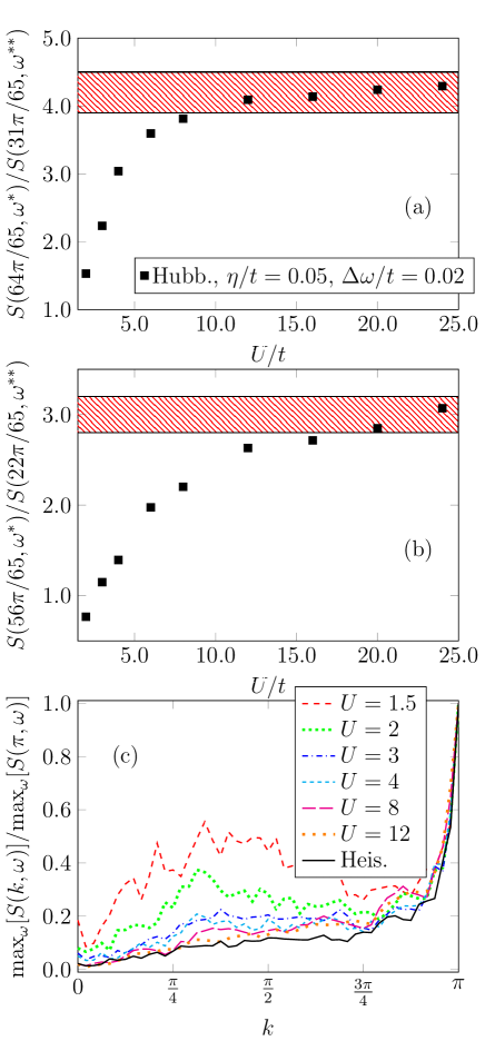
Figure 3: (Color online) Panel (a): Peak to peak ratio $S(64\pi/65,\omega^{*})/S(31\pi/65,\omega^{**})$ as a function of $U/t$ for the Hubbard model on a chain of $L=64$ sites. The ratio obtained for the Heisenberg model is indicated by a dashed (red) region, compatible with the error induced by the extrinsic broadening $\eta/J=0.05$ and our resolution in momentum space $k$ (due to finite system size effects). $\omega^{*}$ is the location of the peak maximum for $k=64\pi/65$, $\omega^{**}$ for $k=31\pi/65$. Panel (b): Peak to peak ratio $S(64\pi/65,\omega^{*})/S(31\pi/65,\omega^{**})$ as a function of $U/t$. Here, $\omega^{*}$ is the location of the peak maximum for $k=56\pi/65$, $\omega^{**}$ for $k=22\pi/65$. Panel (c): Peak to peak ratio between the maxima in frequency of the spectrum $max_{\omega}[S(k,\omega)]$ and the maximum of the spectrum at $k=\pi$ as a function of $k$. Hubbard chains of $L=64$ sites and different $U$ values are considered, together with the same quantity obtained from the Heisenberg model.

IV Two-leg Ladders

This section describes the properties of $S(k,\omega)$ for the same models studied in the previous section but in a different geometry—the two leg ladder.

IV.1 Antiferromagnetic Heisenberg ladder

This section addresses the magnetic excitation spectrum for the spin-$1/2$ Heisenberg model on a two-leg ladder. In eq. (3), the intra-leg coupling $J_{i,j}=J_{x}$ if $i$ and $j$ are nearest neighbors along the $x$ (long) direction; $J_{i,j}=J_{y}$ if $i$ and $j$ are neighbors along the $y$ (short) direction, with $J_{y}$ the inter-leg exchange coupling. We assume that $J_{x},J_{y}>0$ and in particular $J_{x}=1$ as our unit of energy. This model has attracted much attention in the last twenty years because it represents one of the most important paradigms for low dimensional quantum magnetism.

The Heisenberg model behaves completely different on the ladder than on the chain. As seen in sec. III.1, the excitation spectrum is gapless at $k\simeq\pi$ for the spin $1/2$ single chain. However, there exists a spin gap in the ladderDagotto et al. (1992); Barnes et al. (1993); Rice et al. (1993); Balents and Fisher (1996); Gopalan et al. (1994); Shelton et al. (1996); Johnston (1996); Dagotto (1999)—a gap that has been experimentally found.Azuma et al. (1994); Eccleston et al. (1994)

Quantum magnetic systems on ladders have a behavior that can be considered intermediate between the one dimensional and two dimensional physics.Dagotto and Rice (1996); Vuletić et al. (2006) Indeed, both one dimensional and two dimensional magnets have been shown to be gapless. It has also been shown that the physics of half-integer spins ladders depends on the parity of the number of legs.White et al. (1994); Dagotto and Rice (1996)

Figure 4 shows the dynamical spin structure factor for the Heisenberg ladder calculated with the DMRG correction vector methodKühner and White (1999) for different values of the rung exchange coupling $J_{y}$. In the case of the ladder, the dynamical structure factor in momentum space has two components

$$S(k_{x},0,\omega) =\frac{1}{L}\sum_{j=0}^{L/2-1}e^{ik_{x}j}(S(j,0,\omega)+S(j,1,\omega)),$$ (11)

$$S(k_{x},\pi,\omega) =\frac{1}{L}\sum_{j=0}^{L/2-1}e^{ik_{x}j}(S(j,0,\omega)-S(j,1,\omega)),$$

because the momentum in the $y$ direction has only two possible values: $k_{y}=0$ or $k_{y}=\pi$.

The dynamical spin structure factor of the Heisenberg ladder has been calculated both numericallyBarnes et al. (1993); Gopalan et al. (1994); Yang and Haxton (1998); Sushkov and Kotov (1998); Eder (1998); Haga and Suga (2002) and analytically,Balents and Fisher (1996); Damle and Sachdev (1998) both in the weak coupling limit $J_{y}\ll 1$ and in the strong coupling limit $J_{y}\gg 1$.

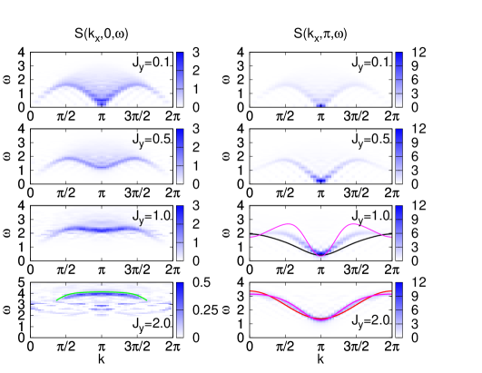
Figure 4: (Color online) Left column panels, from top to bottom: $S(k_{x},0,\omega)$ for the Heisenberg model on a two leg ladder with $L=48\times 2$ sites ($J_{x}=1$), for different values of $J_{y}=0.1,0.5,1.0,2.0$. As before, $m=600$ states are kept in the DMRG simulations. Right column panels: $S(k_{x},\pi,\omega)$ for the same set of parameters described above. In the panel for $J_{y}=1$ the dashed line represents the function $\omega_{gap}(k_{x})$ in eq. (12) obtained in ref. Barnes et al., 1993. The solid lines represent the gap dispersion obtained in the plaquette basis in ref. Piekarewicz and Shepard, 1998. In the panel for $J_{y}=2$ the dashed line represent eq. (12), while the solid line is the gap expression to the 4th order in the strong coupling perturbation theory.

A simple description of the gap physics can be grasped when the strong rung coupling limit $J_{y}\gg J_{x}$ is considered. Following ref. Barnes et al., 1993, a finite spin gap equal to $J_{y}$ in the spectrum of spin excitations obviously appears in the dimer limit, when $J_{x}=0$. Spin excitations can only be produced by promoting a rung singlet to a triplet at the energy cost $J_{y}$. These local excitations are able to propagate along the ladder due to the perturbation given by the exchange coupling along the legs. Using degenerate perturbation theory in the subspace with one rung promoted to triplet and normal perturbation theory on the non-degenerate ground state, one can calculate to order $O(J^{2}_{x}/J_{y})$ the singlet-triplet dispersion relation

$$\omega_{gap}(k_{x})=J_{y}\left[1+\frac{J_{x}}{J_{y}}\cos(k_{x})+\frac{3}{4}\left(\frac{J_{x}}{J_{y}}\right)^{2}\right],$$ (12)

where $J_{x}$ has been reintroduced for the expression to have consistent energy units, and to show that the expansion is in $J_{x}/J_{y}$. This gap implies that the spins show no long-range order. They usually form singlets on the rungs and one verifies numerically that the spin correlation decays exponentially with distance along the legs.Dagotto et al. (1992); White et al. (1994)

Reference Piekarewicz and Shepard, 1998 carries out the strong coupling expansion analytically, including higher order terms, and comparing the dimer and plaquette bases. The authors of ref. Piekarewicz and Shepard, 1998 calculate the ground state energy and the spin gap to 7th order in the parameter $\lambda\equiv J_{x}/J_{y}$, and the gap dispersion up to 4th order. They estimate a radius of convergence $\lambda_{c}=0.8$ for the pertubative expansion by starting from a rung basis, and conclude that perturbative expansions in the rung basis are unsuitable for dealing with the physically interesting case of isotropic ladders ($\lambda=1$). They have explored also the perturbative expansion in a $2\times 2$ plaquette basis, showing that the radius of convergence of the perturbative series can be extended to $\lambda_{c}=1.25$, providing a reliable perturbative approach for the isotropic case ($\lambda=1$). In the isotropic case, figure 4 shows the gap dispersion obtained in ref. Piekarewicz and Shepard, 1998 in the plaquette basis. For $J_{y}=2$, we have included a curve indicating the dispersion obtained in ref. Piekarewicz and Shepard, 1998 to 4th order of perturbation theory in the rung basis.

Figure 4 shows that eq. (12) describes very well the $k_{y}=\pi$ component of the dynamical spin structure factor $S(k_{x},\pi,\omega)$. A strong-coupling calculation reveals that a spin $S=1$ two-particle bound state between two triplets is a possible excitation of the system.Damle and Sachdev (1998) This leads to the presence of a band in the spectrum $S(k_{x},0,\omega)$ with a finite range of values of momentum transfer $k_{x}$. The dispersion of this band of bound states is almost flat, in agreement with the analytic expression $\omega_{2triplet}(k)$ of ref. Zheng et al., 2001.

IV.2 Hubbard model and Comparison to Heisenberg

We now consider a Hubbard model on a two leg ladder geometry. In this case, the hopping interaction parameters appearing in eq. (9) for the two-leg ladder geometry are as follows: the intra-leg hopping $t_{i,j}=t_{(i_{x},i_{y}),(j_{x},i_{y})}=t_{x}$ is non zero if $i_{x}$ and $j_{x}$ are nearest neighbors on leg $i_{y}=0$ and $i_{y}=1$. Furthermore, $t_{(i_{x},0),(i_{x},1)}=t_{y}$ is the rung hopping. Hubbard ladders are considered as an easier starting point to study the properties of the full two dimensional Hubbard model.Dagotto and Rice (1996) According to a bosonization approach,Balents and Fisher (1996); Fabrizio et al. (1992) the phases of the model can be identified by the number of gapless spin and charge modes, with the possibility of having up to two gapless modes in each sector. It has been shown that at half-filling the Hubbard model can be found in a “C0S0” phase, where all the charge and spin modes are gapped. It is however far from obvious that a bosonization picture, which is strictly valid when $U\ll t_{x}$ and at any value of the rung hopping $t_{y}$, could completely explain the physics of the problem. Comparison between analytical and DMRG calculations has been performed in ref. White et al., 2002. Reference Noack et al., 1996 studies the ground state properties of the model with DMRG, and reports that phase separation is not found in the Hubbard ladder. It also provides evidence that the Hubbard model at half-filling, $n=1$, is a spin liquid insulator for $t_{y}<2$ at any value of $U$, while it is a band insulator for $t_{y}>2$. A sharp transition between the two phases turns into a smooth crossover as $U$ is increased.

Unless otherwise stated, in this work we will consider the symmetric $t_{x}=t_{y}=1$ case at half electronic filling, where the presence of the spin liquid insulator phase implies that the spin-spin correlation function decays exponentially from the center of the ladder, inducing a gap in the spin sector of the theory. Away from half-filling, pairing or charge-density wave correlations could be dominant. As suggested by the early considerations on Heisenberg and $t-J$ model ladders, a DMRG study has recently confirmed that superconducting correlations become dominant in the limit of very small doping.Dolfi et al. (2015) A recent study analyzed the ground state and spectral properties of an asymmetric Hubbard ladder,Abdelwahab et al. (2015) of interest in the context of superconducting chains deposited on metallic surfaces. The dynamical properties of the model have mostly been investigated in the half-filled case.Shelton et al. (1996); Schmidt and Uhrig (2005) Away from half-filling, less can be found in the literature. We should mention a Monte Carlo studyJeckelmann et al. (1998) and an exact diagonalization study on a t-J ladder.Poilblanc et al. (2004) Reference Essler and Konik, 2007 uses the connection between the SO(6) Gross-Neveu model and doped Hubbard ladder to study the spin dynamical structure factor. Moreover, several low energy analytic descriptions based on bosonization and generalized symmetries can be found in the literature. These studies have focused on the effect of Umklapp processes opening a gap in the excitation spectrum in the weak coupling undopedLin et al. (1998); Konik and Ludwig (2001); Tsuchiizu and Furusaki (2002); Wu et al. (2003) and doped cases.Robinson et al. (2012)

In the present paper we study the $S(k_{x},k_{y},\omega)$ of the Hubbard ladder with the DMRG using the Krylov approach developed in ref. Nocera and Alvarez, 2016. In the following, we shall consider $t_{x}=1$ as energy unit.

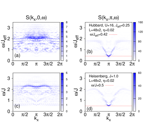
Figure 5: (Color online) Left column: $S(k_{x},0,\omega)$ component for two leg ladder Hubbard (a) model with $L=48\times 2$ sites at half-filling, for $t_{y}=t_{x}=1$ and $U=16$. Panel (c) shows the spectrum for a Heisenberg ladder with $L=48\times 2$ sites and for $J_{x}=J_{y}=1$. In the DMRG simulations, $\eta=\Delta\omega=0.02$ has been considered, and up to $m=1000$ DMRG states have been kept in the numerical simulations. Right column: $S(k_{x},\pi,\omega)$ component of the spectrum for the same parameter values of the left column.

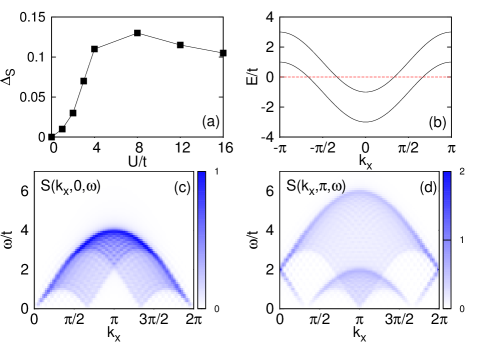
Figure 6: (Color online) Panel (a): Spin gap as a function of the on-site Coulomb repulsion $U$ extracted from the dynamical spin structure factors for a two leg Hubbard ladder with $L=32\times 2$ sites at half-filling. Results agree very well with those obtained in ref. Noack et al., 1996. Panel (b): Non-interacting band structure. Panels (c) and (d): analytical calculation of the dynamical spin structure factor ($\eta=0.02$) for a Hubbard ladder with $L=48\times 2$ sites at half-filling, for $t_{y}=t_{x}=1$ and $U=0.0$.

Panels (a) and (b) of fig. 5 show the two components of the dynamical spin structure factor of a $48\times 2$ ladder with open boundary conditions and $U=16$. In the limit of large on-site Coulomb repulsion, the magnetic excitation spectrum of the Hubbard model is very similar to that of the Heisenberg; this is true for any geometry and is the reason why the spectrum is plotted as a function of the quantity $\omega/J_{\text{eff}}$, where the effective exchange coupling constant is $J_{\text{eff}}=4t_{y}^{2}/U$.

For comparison, panels (c-d) of the same figure show the $S(k_{x},k_{y},\omega)$ of an isotropic Heisenberg ladder with $J_{x}=J_{y}$ of the same system size. Both the $k_{y}=0$ and the $k_{y}=\pi$ branches of the spectrum of the two models show a strong similarity, especially at sufficiently low momenta, $|k_{x}-\pi|<\pi/2$. The $k_{y}=0$ component of the spectrum is dominated by an almost flat band of two-triplet bound states, which has robust intensity only for a finite range of momentum transfer $k_{x}$.Damle and Sachdev (1998); Zheng et al. (2001) The deviations from a pure Heisenberg model behavior can be appreciable mainly in the spectral weight distribution, which is concentrated at lower momentum transfer in the Hubbard case. In the $k_{y}=\pi$ component, the spin gap of the Heisenberg model $\omega_{gap}\simeq 0.5$ is well reproduced by the Hubbard result $\omega_{gap}\simeq 0.42$. Even when $U/(4t)=4\gg 1$, deviations from a pure Heisenberg behavior are noticeable at large momentum transfers, $|k_{x}|>\pi/2$.

In order to verify the accuracy of our DMRG technique, panel (a) of fig. 6 shows the spin gap extracted from the magnetic excitation spectra calculated with DMRG for a Hubbard ladder of $L=32\times 2$ sites as a function of $U$; very good agreement with the ground stated DMRG results of ref. Noack et al., 1996 is obtained.

Before presenting the results for the interacting Hubbard ladder, it is instructive to analyze the properties of the dynamical spin structure factor of a non interacting Hubbard ladder, $U=0$. The spectrum of the Hamiltonian can be described in terms of bonding ($-$) and antibonding ($+$) bands

$$\epsilon_{a/b}(k_{x})=-2t_{x}\cos(k_{x})\mp t_{y},$$ (13)

as shown in panel (b) of figure 6. At a given filling $n$ both bands are filled by electrons if the ratio $t_{y}/t_{x}$ is less than the critical value $(t_{y}/t_{x})_{c}=1-\cos(\pi n)$. At half-filling, $n=1$, the system is a band insulator for $t_{y}/t_{x}>2$, with a gap equal to $2(t_{y}-2t_{x})$, and a two-band metal otherwise. There are four Fermi points: $\pm k_{F_{1}}$ for the bonding, and $\pm k_{F_{2}}$ for the anti-bonding bands; see panel (b) of fig. 6. At half-filling $n=1$, one has $k_{F_{1}}+k_{F_{2}}=\pi$ with $k_{F_{1}}=\pi/3$ and $k_{F_{2}}=2\pi/3$.

Panels (c) and (d) of fig. 6 show the $S(k_{x},k_{y},\omega)$ for a non-interacting isotropic ladder with $L=48\times 2$; $t_{y}=t_{x}=1$ is assumed as unit of energy. The right panel shows the band structure with bonding and anti-bonding bands. When the rung hopping is zero, $t_{y}=0$, then the $0$ and $\pi$ components of the spin spectrum are equal to each other and $k_{F_{1}}=k_{F_{2}}$, reducing to the case of a single chain. When the hopping $t_{y}$ is increased, the $0$ and $\pi$ components of the spin spectrum behave differently, because they encode different excitation processes of the spins. Indeed, the processes described by the $S(k_{x},0,\omega)$ include intraband spin excitations, analogous to the single chain $S(k,\omega)$, with low energy gapless contributions at $k_{x}\simeq 0$ and $k_{x}\simeq 2k_{F_{1/2}}$. In contrast, the processes described by the $S(k_{x},\pi,\omega)$ correspond to interband transitions between bonding and anti-bonding bands and viceversa, with characteristic low energy gapless contributions at $k_{x}\simeq\Delta_{\pm}$, where $\Delta_{\pm}=|k_{F_{1}}|\pm|k_{F_{2}}|$. Keeping in mind the above observation, panel (c) in fig. 6 is readily understood: low energy spin excitations at $k_{x}\simeq 2k_{F_{1}}=2(\pi-k_{F_{2}})$, and $k_{x}\simeq 2k_{F_{2}}=2(\pi-k_{F_{1}})$, together with the usual $k_{x}\simeq 0$ contributions. Except for $t_{y}=2$, where there are no possible intra-band spin excitations, the spectrum upper bound is independent of $t_{y}$, being $4t_{x}$. The spectral weight of the $S(k_{x},0,\omega)$ is concentrated at the upper boundary, which follows a sinusoidal behavior equal to that observed in the chain’s case.

We now discuss the $\pi$ component of the spectrum, reported in panel (d) of fig. 6. For $t_{y}>0$, the sinusoidal upper boundary of the spectrum at $t_{y}=0$ splits into two arcs—arcs separated in frequency by a quantity equal to the bonding-anti-bonding gap, $g=2(t_{y}-2t_{x})$. Concurrently, characteristic low energy gapless contributions at $k_{x}\simeq\Delta_{\pm}$ appear in the spectrum. As opposed to the $k_{y}=0$ case, the upper bound of the spectrum increases proportionally to $t_{y}$, because of processes exciting spin and charges from the bottom of the bonding band to the top of the anti-bonding band. As also observed in panel (c) of fig. 6, the spectrum of the non-interacting case, $U=0$, at $(k_{x}=\pi,k_{y}=0)$ is gapped up to $\omega_{gap}/(4t)\simeq 0.5$, because intra-band excitation with momentum transfer $k_{x}=\pi$ are not possible due to the band structure topology. For the same reason, electronic inter-band excitations are possible instead, and no gap is observed in the $(k_{x}=\pi,k_{y}=\pi)$ cut of the spectrum; see panel (d) of fig. 6.

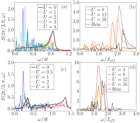
Figure 7: (Color online) Cuts of the spin dynamical structure factors $S(2\pi/3,0,\omega)$ (panels a and b) and $S(2\pi/3,\pi,\omega)$ (panels c and d) for a system with $L=32\times 2$ sites as a function of $\omega/(4t)$ (panel a and c) and $\omega/J_{\text{eff}}$ (panel b and d), at different values of $U$. As in the chain case, we have assumed $J_{\text{eff}}=4t^{2}_{y}/U$. In the DMRG simulations, $\eta=0.02t$ has been considered for the Hubbard model while $\eta=0.02J$ for Heisenberg, with $\Delta\omega=0.01$ and with up to $m=1000$ states kept in DMRG.

We are now ready to discuss the results for an interacting Hubbard ladder, and compare the results to the Heisenberg model. Figure 7 shows cuts of the $k_{y}=0$ and $k_{y}=\pi$ branches of the magnetic excitation spectrum of a Hubbard ladder at $k_{x}=2\pi/3$ as a function of $U$. The choice of $k_{x}=2\pi/3$ is motivated by the gapless behavior observed in the spectrum at $(2\pi/3,0)$ and $(2\pi-2\pi/3,0)$ for $U=0$. Figure 7 shows a redistribution of spectral weight to lower energy at those $k$ points that are gapless in the non-interacting case. We have already seen this redistribution in the case of the chain. The $k_{y}=0$ branch of the spectrum, reported in panel (a) of fig. 7, shows exactly this behavior. The peak at $\omega/(4t)\simeq 0.9$ is gradually suppressed by spectral weight redistribution at lower energy going from $U=0$ to $U=2$. The latter develops a gapped low-energy peak around $\omega/(4t)\simeq 0.1$. The cuts obtained for $U=3$ and $U=4$ have already a pronounced Heisenberg like behavior, with a much suppressed high-energy spectrum and the weight concentrated around $\omega/(4t)\simeq 0.1$. The satellite spectral peaks are due to finite size effects and to the choice of a small $\eta=0.02t$. The cuts obtained by increasing even further the Hubbard repulsion $U$ are shown in panel (b) of fig.7. Here, one can clearly see that the results approach a Heisenberg like behavior, characterized by a single peak at $\omega/J\simeq 2.4$. In this panel, as in the case of the chains, the cuts are plotted against the ratio $\omega/J_{\text{eff}}$, where $J_{eff}=4t_{y}^{2}/U$.

Panels (c) and (d) of figure 7 show the cuts of the $k_{y}=\pi$ branch of the spectrum for different values of $U$ as in the previous panels. The redistribution of spectral weight to low frequency is also observed here increasing the Coulomb repulsion from $U=0$ to $U=1$. Again, the cut of the spectrum for $U=2$ presents a suppression of spectral weight at large frequency and develops a spectral peak resembling a Heisenberg-like behavior at $\omega/(4t)\simeq 0.25$. The crossover to a Heisenberg-like behavior is almost complete at $U=3$; see the dashed-dotted (blue) curve in panel (c). The spectrum approaches the Heisenberg limit for very large Coulomb repulsion; see panel (d) of fig. 7. As in the chains’ case, the width of the shaded region has been estimated as described in section III.2 before eq. 10.

Figure 8 shows the ratio of spectral intensities between the two branches of the spectrum at $k_{x}=2\pi/3$. Figure 8 provides a quantitative criterion to decide where a particular quasi-one dimensional material with ladder structure is located in parameter space with regards to the strength of its Hubbard coupling. Similar to the case of chains studied in the previous section, the peak ratio evolves continuously with increasing $U/t$, and only slowly converges to the Heisenberg limit. However, qualitatively a Heisenberg-like magnetic excitation spectrum is found for the Hubbard model already at $U/t\sim 2$, which for ladders is a relatively small coupling regime considering that the electronic bandwidth is $W=6t$.

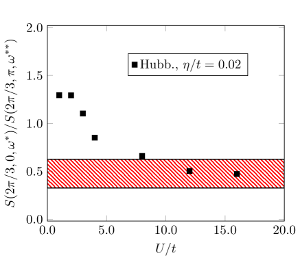
Figure 8: (Color online) Peak to peak ratio $S(2\pi/3,0,\omega^{*})/S(2\pi/3,\pi,\omega^{**})$ as a function of $U/t$ for the Hubbard model on a ladder of $L=32\times 2$ sites. The ratio obtained for the Heisenberg model is indicated by a dashed (red) region, compatible with the error induced by the extrinsic broadening $\eta/J=0.02$ and our resolution in momentum space $k$ (due to finite system size effects). $\omega^{*}$ is the location of the peak maximum for $(k_{x},k_{y})=(2\pi/3,0)$, $\omega^{**}$ for $(k_{x},k_{y})=(2\pi/3,\pi)$. Same parameters’ choice as in fig. 7.

In the supplemental material, which can be found at https://drive.google.com/open?id=0B4WrP8cGc5JHWXhkcG5wNzk5TDA, we complement the study of ladders reported in this section by analyzing the cuts of the two branches of the magnetic excitation spectrum at the special case $k_{x}=\pi$, where similar results are obtained.

V Summary and Conclusions

In this work, we have compared the dynamical spin structure factor of two well known models of strongly correlated materials, the Heisenberg and the Hubbard models. By evaluating the dynamical spectra we have shown that, both for chains and ladders, it is possible to quantitatively identify the range of the on-site repulsion strenghts where the Hubbard model resembles that of the Heisenberg model. Surprisingly, the spectra of the Hubbard model shows qualitative features that resemble Heisenberg behavior already at relatively small values of $U$, in particular $U/t\simeq 2-3$ for both chains and ladders. This explains the success of the Heisenberg model in describing such a wide range of compounds, even including metals such as iron. However, $ratios$ of intensities at various momenta converge slowly to the Heisenberg limit and provide an excellent criteria to evaluate the precise value of $U/t$ from neutron data.

In fact, current methods and tools of analysis of inelastic neutron scattering dataArnold et al. (2014) allow for a quantitative evaluation of the magnetic excitation spectrum that make possible a direct comparison of the relative intensities of the magnetic excitation spectra at different wave vectors, as proposed in this paper. This comparison will bring considerable light about the applicability of approaches based either on a Heisenberg or a Hubbard model. This is in contrast to the earlier days of neutron studies, when the information obtained from inelastic neutron scattering was largely limited to the peak energy of an excitation, which was plotted against the wave vector in order to present the corresponding dispersion relation; see for example ref. Collins et al., 1969. Another important information that is currently available in the neutron inelastic scattering spectra is the “intrinsic” broadening of the excitations; this provides essential information about the lifetime of the excitations. The intrinsic broadening of the experimentally observed magnetic excitations can be evaluated taking into consideration proper corrections for the instrumental resolution. Future efforts in calculations similar to those in this paper could, in principle, account for the broadening mechanisms of the excitations, and provide additional information that could be directly compared to neutron scattering experiments.

References

- Lake et al. (2013) B. Lake, D. A. Tennant, J.-S. Caux, T. Barthel, U. Schollwöck, S. E. Nagler, and C. D. Frost, Phys. Rev. Lett. 111, 137205 (2013), URL http://link.aps.org/doi/10.1103/PhysRevLett.111.137205.
- Collins et al. (1969) M. F. Collins, V. J. Minkiewicz, R. Nathans, L. Passell, and G. Shirane, Phys. Rev. 179, 417 (1969), URL http://link.aps.org/doi/10.1103/PhysRev.179.417.
- Perring et al. (1991) T. Perring, A. Boothroyd, D. M. Paul, A. Taylor, R. Osborn, R. J. Newport, J. Blackman, and H. Mook, Journal of Applied Physics 69, 6219 (1991).
- Giamarchi (2004) T. Giamarchi, Quantum physics in one dimension (Clarendon Press, Oxford; 1 edition (February 26, 2004), 2004).
- Haldane (1983) F. D. M. Haldane, Phys. Rev. Lett. 50, 1153 (1983), URL http://link.aps.org/doi/10.1103/PhysRevLett.50.1153.
- Dagotto et al. (1992) E. Dagotto, J. Riera, and D. Scalapino, Phys. Rev. B 45, 5744 (1992), URL http://link.aps.org/doi/10.1103/PhysRevB.45.5744.
- White et al. (1994) S. R. White, R. M. Noack, and D. J. Scalapino, Phys. Rev. Lett. 73, 886 (1994), URL http://link.aps.org/doi/10.1103/PhysRevLett.73.886.
- Dagotto and Rice (1996) E. Dagotto and T. M. Rice, Science 271, 618 (1996), eprint http://www.sciencemag.org/content/271/5249/618.full.pdf, URL http://www.sciencemag.org/content/271/5249/618.abstract.
- Maekawa (1996) S. Maekawa, Science 273, 1515 (1996).
- Tranquada et al. (2004) J. Tranquada, H. Woo, T. Perring, H. Goka, G. Gu, G. Xu, M. Fujita, and K. Yamada, Nature 429, 534 (2004).
- Azuma et al. (1994) M. Azuma, Z. Hiroi, M. Takano, K. Ishida, and Y. Kitaoka, Physical Review Letters 73, 3463 (1994).
- Dai et al. (2012) P. Dai, J. Hu, and E. Dagotto, Nature Physics 8, 709 (2012).
- Dagotto (2013) E. Dagotto, Reviews of Modern Physics 85, 849 (2013).
- Takahashi et al. (2015) H. Takahashi, A. Sugimoto, Y. Nambu, T. Yamauchi, Y. Hirata, T. Kawakami, M. Avdeev, K. Matsubayashi, F. Du, C. Kawashima, et al., Nature materials 14, 1008 (2015).
- Patel et al. (2016) N. D. Patel, A. Nocera, G. Alvarez, R. Arita, A. Moreo, and E. Dagotto, arXiv preprint arXiv:1604.03621 (2016).
- Duan et al. (2003) L.-M. Duan, E. Demler, and M. D. Lukin, Phys. Rev. Lett. 91, 090402 (2003), URL http://link.aps.org/doi/10.1103/PhysRevLett.91.090402.
- García-Ripoll et al. (2004) J. J. García-Ripoll, M. A. Martin-Delgado, and J. I. Cirac, Phys. Rev. Lett. 93, 250405 (2004), URL http://link.aps.org/doi/10.1103/PhysRevLett.93.250405.
- Zapf et al. (2014) V. Zapf, M. Jaime, and C. Batista, Reviews of Modern Physics 86, 563 (2014).
- Thielemann et al. (2009) B. Thielemann, C. Rüegg, H. M. Rønnow, A. M. Läuchli, J.-S. Caux, B. Normand, D. Biner, K. W. Krämer, H.-U. Güdel, J. Stahn, et al., Phys. Rev. Lett. 102, 107204 (2009), URL http://link.aps.org/doi/10.1103/PhysRevLett.102.107204.
- Bouillot et al. (2011) P. Bouillot, C. Kollath, A. M. Läuchli, M. Zvonarev, B. Thielemann, C. Rüegg, E. Orignac, R. Citro, M. Klanjšek, C. Berthier, et al., Physical Review B 83, 054407 (2011).
- Schmidiger et al. (2012) D. Schmidiger, P. Bouillot, S. Mühlbauer, S. Gvasaliya, C. Kollath, T. Giamarchi, and A. Zheludev, Phys. Rev. Lett. 108, 167201 (2012), URL http://link.aps.org/doi/10.1103/PhysRevLett.108.167201.
- Yu et al. (2012) R. Yu, L. Yin, N. S. Sullivan, J. Xia, C. Huan, A. Paduan-Filho, N. F. Oliveira Jr, S. Haas, A. Steppke, C. F. Miclea, et al., Nature 489, 379 (2012).
- Coldea et al. (2001) R. Coldea, S. M. Hayden, G. Aeppli, T. G. Perring, C. D. Frost, T. E. Mason, S.-W. Cheong, and Z. Fisk, Phys. Rev. Lett. 86, 5377 (2001), URL http://link.aps.org/doi/10.1103/PhysRevLett.86.5377.
- Bhaseen et al. (2005) M. J. Bhaseen, F. H. L. Essler, and A. Grage, Phys. Rev. B 71, 020405 (2005), URL http://link.aps.org/doi/10.1103/PhysRevB.71.020405.
- Essler et al. (2003) F. Essler, H. Frahm, F. Göhmann, A. Klümper, and V. Korepin, The one-dimensional Hubbard model (Cambridge University Press, 2003).
- White (1992) S. R. White, Phys. Rev. Lett. 69, 2863 (1992), URL http://link.aps.org/doi/10.1103/PhysRevLett.69.2863.
- White (1993) S. R. White, Phys. Rev. B 48, 10345 (1993), URL http://link.aps.org/doi/10.1103/PhysRevB.48.10345.
- Benthien and Jeckelmann (2007) H. Benthien and E. Jeckelmann, Phys. Rev. B 75, 205128 (2007), URL http://link.aps.org/doi/10.1103/PhysRevB.75.205128.
- Kühner and White (1999) T. D. Kühner and S. R. White, Phys. Rev. B 60, 335 (1999), URL http://link.aps.org/doi/10.1103/PhysRevB.60.335.
- Nocera and Alvarez (2016) A. Nocera and G. Alvarez, arXiv preprint arXiv:1607.03538 (2016).
- Lin (1990) H. Q. Lin, Phys. Rev. B 42, 6561 (1990), URL http://link.aps.org/doi/10.1103/PhysRevB.42.6561.
- Hallberg (1995) K. A. Hallberg, Phys. Rev. B 52, R9827 (1995), URL http://link.aps.org/doi/10.1103/PhysRevB.52.R9827.
- Karbach et al. (1997) M. Karbach, G. Müller, A. H. Bougourzi, A. Fledderjohann, and K.-H. Mütter, Phys. Rev. B 55, 12510 (1997), URL http://link.aps.org/doi/10.1103/PhysRevB.55.12510.
- Müller et al. (1981) G. Müller, H. Thomas, H. Beck, and J. C. Bonner, Phys. Rev. B 24, 1429 (1981), URL http://link.aps.org/doi/10.1103/PhysRevB.24.1429.
- Affleck (1998) I. Affleck, Journal of Physics A: Mathematical and General 31, 4573 (1998), URL http://stacks.iop.org/0305-4470/31/i=20/a=002.
- Mourigal et al. (2013) M. Mourigal, M. Enderle, A. Klöpperpieper, J.-S. Caux, A. Stunault, and H. M. Rønnow, Nature Physics 9, 435 (2013).
- Haldane and Zirnbauer (1993) F. D. M. Haldane and M. R. Zirnbauer, Phys. Rev. Lett. 71, 4055 (1993), URL http://link.aps.org/doi/10.1103/PhysRevLett.71.4055.
- Barnes et al. (1993) T. Barnes, E. Dagotto, J. Riera, and E. S. Swanson, Phys. Rev. B 47, 3196 (1993), URL http://link.aps.org/doi/10.1103/PhysRevB.47.3196.
- Rice et al. (1993) T. Rice, S. Gopalan, and M. Sigrist, EPL (Europhysics Letters) 23, 445 (1993).
- Balents and Fisher (1996) L. Balents and M. P. A. Fisher, Phys. Rev. B 53, 12133 (1996), URL http://link.aps.org/doi/10.1103/PhysRevB.53.12133.
- Gopalan et al. (1994) S. Gopalan, T. M. Rice, and M. Sigrist, Phys. Rev. B 49, 8901 (1994), URL http://link.aps.org/doi/10.1103/PhysRevB.49.8901.
- Shelton et al. (1996) D. G. Shelton, A. A. Nersesyan, and A. M. Tsvelik, Phys. Rev. B 53, 8521 (1996), URL http://link.aps.org/doi/10.1103/PhysRevB.53.8521.
- Johnston (1996) D. C. Johnston, Phys. Rev. B 54, 13009 (1996), URL http://link.aps.org/doi/10.1103/PhysRevB.54.13009.
- Dagotto (1999) E. Dagotto, Reports on Progress in Physics 62, 1525 (1999).
- Eccleston et al. (1994) R. S. Eccleston, T. Barnes, J. Brody, and J. W. Johnson, Physical Review Letters 73, 2626 (1994).
- Vuletić et al. (2006) T. Vuletić, B. Korin-Hamzić, T. Ivek, S. Tomić, B. Gorshunov, M. Dressel, and J. Akimitsu, Physics Reports 428, 169 (2006).
- Yang and Haxton (1998) D. B. Yang and W. C. Haxton, Phys. Rev. B 57, 10603 (1998), URL http://link.aps.org/doi/10.1103/PhysRevB.57.10603.
- Sushkov and Kotov (1998) O. P. Sushkov and V. N. Kotov, Phys. Rev. Lett. 81, 1941 (1998), URL http://link.aps.org/doi/10.1103/PhysRevLett.81.1941.
- Eder (1998) R. Eder, Phys. Rev. B 57, 12832 (1998), URL http://link.aps.org/doi/10.1103/PhysRevB.57.12832.
- Haga and Suga (2002) N. Haga and S.-i. Suga, Phys. Rev. B 66, 132415 (2002), URL http://link.aps.org/doi/10.1103/PhysRevB.66.132415.
- Damle and Sachdev (1998) K. Damle and S. Sachdev, Phys. Rev. B 57, 8307 (1998), URL http://link.aps.org/doi/10.1103/PhysRevB.57.8307.
- Piekarewicz and Shepard (1998) J. Piekarewicz and J. R. Shepard, Phys. Rev. B 58, 9326 (1998), URL http://link.aps.org/doi/10.1103/PhysRevB.58.9326.
- Zheng et al. (2001) W. Zheng, C. J. Hamer, R. R. P. Singh, S. Trebst, and H. Monien, Phys. Rev. B 63, 144410 (2001), URL http://link.aps.org/doi/10.1103/PhysRevB.63.144410.
- Fabrizio et al. (1992) M. Fabrizio, A. Parola, and E. Tosatti, Phys. Rev. B 46, 3159 (1992), URL http://link.aps.org/doi/10.1103/PhysRevB.46.3159.
- White et al. (2002) S. R. White, I. Affleck, and D. J. Scalapino, Phys. Rev. B 65, 165122 (2002), URL http://link.aps.org/doi/10.1103/PhysRevB.65.165122.
- Noack et al. (1996) R. Noack, S. White, and D. Scalapino, Physica C: Superconductivity 270, 281 (1996), ISSN 0921-4534, URL http://www.sciencedirect.com/science/article/pii/S0921453496005151.
- Dolfi et al. (2015) M. Dolfi, B. Bauer, S. Keller, and M. Troyer, Phys. Rev. B 92, 195139 (2015), URL http://link.aps.org/doi/10.1103/PhysRevB.92.195139.
- Abdelwahab et al. (2015) A. Abdelwahab, E. Jeckelmann, and M. Hohenadler, Phys. Rev. B 91, 155119 (2015), URL http://link.aps.org/doi/10.1103/PhysRevB.91.155119.
- Schmidt and Uhrig (2005) K. P. Schmidt and G. S. Uhrig, Modern Physics Letters B 19, 1179 (2005), URL http://www.worldscientific.com/doi/abs/10.1142/S0217984905009237.
- Jeckelmann et al. (1998) E. Jeckelmann, D. J. Scalapino, and S. R. White, Phys. Rev. B 58, 9492 (1998), URL http://link.aps.org/doi/10.1103/PhysRevB.58.9492.
- Poilblanc et al. (2004) D. Poilblanc, E. Orignac, S. R. White, and S. Capponi, Phys. Rev. B 69, 220406 (2004), URL http://link.aps.org/doi/10.1103/PhysRevB.69.220406.
- Essler and Konik (2007) F. H. L. Essler and R. M. Konik, Phys. Rev. B 75, 144403 (2007), URL http://link.aps.org/doi/10.1103/PhysRevB.75.144403.
- Lin et al. (1998) H.-H. Lin, L. Balents, and M. P. A. Fisher, Phys. Rev. B 58, 1794 (1998), URL http://link.aps.org/doi/10.1103/PhysRevB.58.1794.
- Konik and Ludwig (2001) R. Konik and A. W. W. Ludwig, Phys. Rev. B 64, 155112 (2001), URL http://link.aps.org/doi/10.1103/PhysRevB.64.155112.
- Tsuchiizu and Furusaki (2002) M. Tsuchiizu and A. Furusaki, Phys. Rev. B 66, 245106 (2002), URL http://link.aps.org/doi/10.1103/PhysRevB.66.245106.
- Wu et al. (2003) C. Wu, W. V. Liu, and E. Fradkin, Phys. Rev. B 68, 115104 (2003), URL http://link.aps.org/doi/10.1103/PhysRevB.68.115104.
- Robinson et al. (2012) N. J. Robinson, F. H. L. Essler, E. Jeckelmann, and A. M. Tsvelik, Phys. Rev. B 85, 195103 (2012), URL http://link.aps.org/doi/10.1103/PhysRevB.85.195103.
- Arnold et al. (2014) O. Arnold, J.-C. Bilheux, J. Borreguero, A. Buts, S. I. Campbell, L. Chapon, M. Doucet, N. Draper, R. F. Leal, M. Gigg, et al., Nuclear Instruments and Methods in Physics Research Section A: Accelerators, Spectrometers, Detectors and Associated Equipment 764, 156 (2014).
- Lake et al. (2005) B. Lake, D. A. Tennant, and S. E. Nagler, Phys. Rev. B 71, 134412 (2005), URL http://link.aps.org/doi/10.1103/PhysRevB.71.134412.