A minimization problem with free boundary related to a cooperative system

Abstract.

We study the minimum problem for the functional

$$\int_{\Omega}\bigl{(}|\nabla\mathbf{u}|^{2}+Q^{2}\chi_{\{|\mathbf{u}|>0\}}\bigr{)}dx$$

with the constraint $u_{i}\geq 0$ for $i=1,\cdots,m$ where $\Omega\subset\mathbb{R}^{n}$ is a bounded domain and $\mathbf{u}=(u_{1},\cdots,u_{m})\in H^{1}(\Omega;\mathbb{R}^{m})$.

Using an array of technical tools, from geometric analysis for the free boundaries, we reduce the problem to its scalar counterpart and hence conclude similar results as that of scalar problem. This can also be seen as the most novel part of the paper, that possibly can lead to further developments of free boundary regularity for systems.

1. Introduction

1.1. Background

In the last four decades the regularity theory of free boundary problems has seen an unprecedented surge of developments of new technical devices, that have resulted in solving both old and new problems, unfeasible with earlier techniques. Most of these tools, enrooted in the analysis of minimal surfaces, have been enhanced and undergone major changes and in some cases even being reincarnated. Cavitational flow, Obstacle problem and Thin obstacles are a few among many of those problems, that have been treated successfully with these newly developed tools. It is, however, not until very recently that problems which involve system of equations have been treated from a regularity theory point of view, see [16, 6, 7]. There seems to be lack of a general methodology and approach for analyzing the regularity for systems of free boundary problems. Our intention with this paper is to initiate the study of Cavitational problems where several flows are involved, and interact whenever there is phase transition.

The mathematical model we have chosen to work with is the by-now classical problem of Bernoulli type free boundary, that was treated by the first author with H. Alt [3]. The simplest setting of such a problem asks for properties of the minimizers $\mathbf{u}=(u_{1},\cdots,u_{m})$ of the functional

$$J(\mathbf{u})=\int_{\Omega}\bigl{(}|\nabla\mathbf{u}|^{2}+Q^{2}\chi_{\{|\mathbf{u}|>0\}}\bigr{)}dx$$

over an appropriate Sobolev vector-valued functions, domain $\Omega\subset\mathbb{R}^{n}$, smooth enough $Q$, and boundary values.

Minimizers of this functional describe (optimal) stationary thermal insulation, allowing a prescribed heat loss from the insulating layer. The heat flows in from the boundary of the domain $\Omega$, through a vector function $\mathbf{g}\in H^{1}(\Omega;{\mathbb{R}}^{m})$ on the boundary (boundary data). Each $g_{i}$ gives rise to a potential function $u_{i}$ describing the heat distribution from the data $g_{i}$, and the system has to cost through Dirichlet energy as well as the total volume of heated region. Since this is a system, the latter is described by $|\{|\mathbf{u}|>0\}|$. If the supports of $g_{i}$-s stay far from each other (and data is small enough) then it is reasonable that the system behaves exactly like scalar case, for each $i=1,\cdots,m$. When the supports of $g_{i}$-s come close (or some $g_{i}$-s become large), then naturally the volume of each support $\{u_{i}>0\}$ increases, and at some stage it is less costly to use same insulation layer, i.e. they prefer to share support, and hence $\sup u_{i}=\sup u_{j}$ for some of these $i,j$. Those $g_{i}$ that are still small (and their support stay far from others) will insulate separately. The total heat of the system at each point is given by $\sum u_{i}$, and this is a major difference between our problem and standard scalar problem. A similar model can appear in population dynamics where several species coexist, and overflow the patches. In such models (and many others) each $u_{i}$ may represent a population density (or any quantity given by the system). We refer to Section 6.3 for relation between the supports of $u_{i}$, and for rigorous arguments concerning our discussion here.

Other models of such a problem appears as equilibrium state(s) of cooperative systems, corresponding to reaction-diffusion systems, with high concentration of energy close to the free boundary. Limit of such singularly perturbed problems lead to minimization of our functional. Other related models may appear in shape optimization, where the Dirichlet energy of vector-valued functions are to be minimized, subject to volume constraint of the type $|\{|\mathbf{u}|>0\}|=A>0$, with $|\Omega|>A$, and Dirichlet data on $\partial\Omega$. It is noteworthy that our approach in this paper also applies to the corresponding two-phase problems, as well as singular perturbations, and volume-constrained maps.

Our results are in lines of that of [3] and several of the succeeding papers [2], [20], etc. However, our methodology (besides the obvious preliminary footwork) and strategy is somehow new. For the main regularity theory, instead of working with the system, we use a reduction method to the scalar case with the cost of loosing the regularity of the free boundary condition that is assumed/given in the scalar case. More exactly, our analysis boils down to a weak solution of

$$\Delta u_{i}=w_{i}Q\mathcal{H}^{n-1}\llcorner(\Omega\cap\partial^{*}\{|\mathbf{u}|>0\})\enskip\text{for}\enskip i=1,\cdots,m\text{,}$$

where (see Notation section for definitions)

$$w_{i}(x)=\lim_{y\in\{|\mathbf{u}|>0\},y\to x}\frac{u_{i}(y)}{|\mathbf{u}(y)|}\text{.}$$

In this reformulation the information about the continuity of the Bernoulli boundary condition is lost, since a priori we do not know how regular $w_{i}$ are. The heart of the matter lies in proving the Hölder regularity of the functions $w_{i}$. It should be remarked that this might be seen as the most novel part of of our paper; see Section 7.

In a follow up paper [9] we shall consider this problem in a more general setting, allowing sign change as well as more general integrand (anisotropic as well as degenerate/singular) in our functional.

1.2. Mathematical Setting

Let $\Omega\subset\mathbb{R}^{n}$ be a bounded domain and $m\geq 1$ an integer. Let $Q:\Omega\to\mathbb{R}$ be Lebesgue measurable and there exist constants $Q_{max}\geq Q_{min}>0$ such that $Q_{min}\leq Q\leq Q_{max}$ a.e. in $\Omega$. For $\mathbf{u}\in H^{1}(\Omega;\mathbb{R}^{m})$ let us define

$$J(\mathbf{u})=\int_{\Omega}\bigl{(}|\nabla\mathbf{u}|^{2}+Q^{2}\chi_{\{|\mathbf{u}|>0\}}\bigr{)}dx$$

where

$$|\nabla\mathbf{u}|^{2}=|\nabla u_{1}|^{2}+\cdots+|\nabla u_{m}|^{2}\text{,}$$

here $|\cdot|$ denotes the Euclidean length.

Let $\mathbf{g}\in H^{1}(\Omega;\mathbb{R}^{m})$ such that $g_{i}\geq 0$ a.e. in $\Omega$ for $i=1,\cdots,m$. We consider the minimization problem of the functional $J$ for $\mathbf{u}\in H^{1}(\Omega;\mathbb{R}^{m})$ under the constraint that $\mathbf{u}=\mathbf{g}$ on $\partial\Omega$ and the sign constraints

$$u_{i}\geq 0\enskip\text{a.e. in}\enskip\Omega\enskip\text{for}\enskip i=1,\cdots,m\text{.}$$

Remark 1.

If we change the volume constraint in our functions above, to $\sum_{i}\chi_{\{u_{i}>0\}}$ then the components decouple and we fall back to scalar case for each $i=1,\cdots,m$.

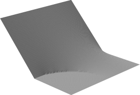
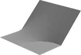
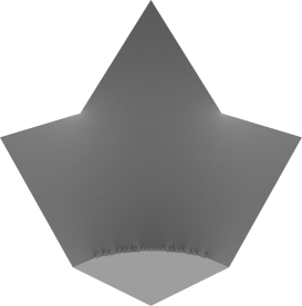
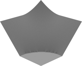
In Figure 1 an example of local minimizer (see Definition 1) is depicted. In this example we have $\Omega=(-1,1)^{2}$, $m=2$, $Q=1$, $g_{1}(x)=x_{2}^{-}$ and $g_{2}(x)=x_{1}^{+}$. Because in this paper the sum of the components of $\mathbf{u}$ and the length of $\mathbf{u}$ will play an important role, we have also depicted these functions.

(a) $u_{1}$

(b) $u_{2}$

(c) $u_{1}+u_{2}$

(d) $|\mathbf{u}|$

Figure 1. Components of a local minimizer $\mathbf{u}$ together with the sum $u_{1}+u_{2}$ and its length $|\mathbf{u}|$.

1.3. Notation

Here we shall line up important notations that are frequently used in this paper.

$C$, $C_{1}$, $C_{2}$	generic constants;
$\chi_{D}$	characteristic function of the set $D$ ($D\subset\mathbb{R}^{n}$);
$\overline{D}$	the closure of $D$;
$\partial D$	boundary of $D$;
$\partial^{*}D$	reduced boundary of $D$;
$\partial_{*}D$	measure theoretic boundary of $D$;
$D^{\circ}$	interior of $D$;
$\sigma$	surface measure;
$|\cdot|$	absolute value, euclidean length of a vector,
	norm of a matrix, Lebesgue measure or surface measure;
$\mathcal{H}^{m}$	$m$-dimensional Hausdorff measure (on $\mathbb{R}^{n}$);
$\|\cdot\|$	norm of functions;
$[\cdot]$	seminorm of functions;
$B_{r}^{m}(x)$	$\bigl{\{}y\in\mathbb{R}^{m}\ |\ |y-x|<r\bigr{\}}$;
$B_{r}(x)$, $B_{r}$, $B$	$B_{r}^{n}(x)$, $B_{r}^{n}(0)$, $B_{1}^{n}(0)$;
$f^{+}$, $f^{-}$	$\max(0,f)$, $\max(0,-f)$;
$\subset\subset$	compactly contained;
$\fint$	integral mean;
$\nu$	outer normal;
$\mu\llcorner A$	measure $\mu$ restricted to the set $A$.

2. Main Results

Let us denote by $\mathcal{A}$ the set of our admissible functions, i.e.

(2.1) $$\mathcal{A}=\Bigl{\{}\mathbf{v}\in H^{1}(\Omega;\mathbb{R}^{m})\enskip\Bigm{|}\enskip\mathbf{v}=g\enskip\text{on}\enskip\partial\Omega\\ \enskip\text{and}\enskip\mathbf{v}_{i}\geq 0\enskip\text{a.e. in}\enskip\Omega\enskip\text{for}\enskip i=1,\cdots,m\Bigr{\}}\text{.}$$

We call $\mathbf{u}\in\mathcal{A}$ an absolute minimizer if $J(\mathbf{u})\leq J(\mathbf{v})$ for all $\mathbf{v}\in\mathcal{A}$.

Theorem 1.

There exists an absolute minimizer of our problem.

For $\mathbf{u},\mathbf{v}\in H^{1}(\Omega;\mathbb{R}^{m})$ let us define the metric $d$ on $H^{1}(\Omega;\mathbb{R}^{m})$ by

(2.2) $$d(\mathbf{u},\mathbf{v}):=\|\mathbf{u}-\mathbf{v}\|_{H^{1}(\Omega;\mathbb{R}^{m})}+\|\chi_{\{|\mathbf{u}|>0\}}-\chi_{\{|\mathbf{v}|>0\}}\|_{L^{1}(\Omega)}\text{.}$$

Definition 1.

We call $\mathbf{u}\in\mathcal{A}$ a local minimizer if there exists $\epsilon>0$ such that $J(\mathbf{u})\leq J(\mathbf{v})$ for $\mathbf{v}\in\mathcal{A}$ with $d(\mathbf{u},\mathbf{v})<\epsilon$.

Theorem 2 (Optimal linear growth).

There exists $C>0$ such that for $\mathbf{u}$ a (local) minimizer and $B_{r}(x)\subset\subset\Omega$ (small balls) if $\overline{B_{r}(x)}\cap\{|\mathbf{u}|=0\}\not=\emptyset$ then

$$\fint_{\partial B_{r}(x)}u_{i}d\sigma\leq CQ_{max}r\enskip\text{for}\enskip i=1,\cdots,m\text{.}$$

In particular, from the linear growth estimate proved in Theorem 2 it follows that $\mathbf{u}$ is Lipschitz continuous, see Corollary 1.

Theorem 3 (Optimal linear nondegeneracy).

Let $\mathbf{u}$ be a (local) minimizer, for $B_{r}(x)\subset\Omega$ (small balls), $0<\rho<1$ (in the case when $n=2$ and $u$ is a local minimizer also small enough $\rho$) and $\overline{B_{\rho r}(x)}\cap\{|\mathbf{u}|>0\}\not=\emptyset$ then

$$\sup_{B_{r}(x)}|\mathbf{u}|\geq cQ_{min}r$$

where $c>0$ depends only on $\rho$.

Theorem 4 (Equation satisfied by each component).

Let $Q$ be a continuous function, then for $\mathcal{H}^{n-1}$ a.e. point $x\in\Omega\cap\partial^{*}\{|\mathbf{u}|>0\}$, $i=1,\cdots,m$ and $\eta>0$ the non-tangential limit

(2.3) $$w_{i}(x)=\lim_{y\in\{|\mathbf{u}|>0\}\cap\{-(y-x)\cdot\nu_{\{|\mathbf{u}|>0\}}(x)\geq\eta\},y\to x}\frac{u_{i}(y)}{|\mathbf{u}(y)|}$$

(here $\nu_{\{|\mathbf{u}|>0\}}(x)$ is the outer normal to $\{|\mathbf{u}|>0\}$ at the point $x$) exists and we have the equations

(2.4) $$\Delta u_{i}=w_{i}Q\mathcal{H}^{n-1}\llcorner(\Omega\cap\partial^{*}\{|\mathbf{u}|>0\})\enskip\text{for}\enskip i=1,\cdots,m\text{.}$$

In the following theorem we prove that around a free boundary point, the set $\{|\mathbf{u}|>0\}$ is a non-tangentially accessible domain. In the Definition 9 a non-tangentially accessible domain, with its associated parameters $M$, $\xi$ and $c$, is defined.

Theorem 5 ($\{|\mathbf{u}|>0\}$ is non-tangentially accessible).

Let $\mathbf{u}$ be a (local) minimizer, for $B_{r_{0}}(x_{0})\subset\Omega$ (small enough) with $x_{0}\in\partial\{|\mathbf{u}|>0\}$, there exists $0<\epsilon_{1}<1$ and $0<\tilde{\epsilon}_{1}<\epsilon_{1}$ such that $B_{\epsilon_{1}r_{0}}(x_{0})\cap\{|\mathbf{u}|>0\}$ is a non-tangentially accessible domain with parameters $M>1$, $\xi=\tilde{\epsilon}_{1}r_{0}$ and $0<c<1$ (where $\epsilon_{1}$, $\tilde{\epsilon}_{1}$, $M$ and $c$ depend only on $n$, $m$, $\frac{Q_{max}}{Q_{min}}$ and additionally on $u$ in the case when $n=2$ and $u$ is a local minimizer).

Definition 2.

For $0<\sigma\leq 1$ and $\nu\in\partial B$ we say that the minimizer $\mathbf{u}$ is $\sigma$-flat in $B_{\rho}(x)\subset\Omega$ in the direction $\nu$ if $x\in\partial\{|\mathbf{u}|>0\}$ and $\mathbf{u}=0$ in $B_{\rho}(x)\cap\{y\ |\ (y-x)\cdot\nu\geq\sigma\rho\}$.

Assume $x_{0}$, $r_{0}$ and $\epsilon_{1}$ to be as in Theorem 5. In Lemma 14 and 15 using the comparison principle for non-tangentially accessible domains (see Lemma 26) we obtain that $w_{i}$ for $i=1,\cdots,m$ are Hölder continuous in $B_{\epsilon_{2}\epsilon_{1}r_{0}}(x_{0})\cap\{|\mathbf{u}|>0\}$ where $0<\epsilon_{2}<1$ depends on the parameters of non-tangentially accessibility which in turn depend on $n$, $m$, $\frac{Q_{max}}{Q_{min}}$ and additionally on $u$ in the case when $n=2$ and $u$ is a local minimizer.

Theorem 6 (Flatness implies regularity).

Let $Q$ be Hölder continuous and $\mathbf{u}$ be a minimizer of our functional. Then there are constants $\alpha>0$, $\beta>0$, $\sigma_{0}>0$, $\tau_{0}>0$ and $C<\infty$ such that if $\mathbf{u}$ is $\sigma$-flat in $B_{\rho}(x_{0})$ in the direction $\nu$ with $\sigma\leq\sigma_{0}$ and $\rho\leq\min(\tau_{0}\sigma^{\frac{2}{\beta}},\frac{1}{2}\epsilon_{2}\epsilon_{1}r_{0})$ then

$$B_{\frac{\rho}{4}}(x_{0})\cap\partial\{|\mathbf{u}|>0\}\enskip\text{is a}\enskip C^{1,\alpha}\enskip\text{surface}$$

(a graph in direction $\nu$ of a $C^{1,\alpha}$ function), and for $x_{1},x_{2}$ on this surface

$$|\nu(x_{1})-\nu(x_{2})|\leq C\sigma\bigl{|}\frac{x_{2}-x_{1}}{\rho}\bigr{|}^{\alpha}\text{.}$$

The constants depend on $n$, $Q_{min}$, $Q_{max}$ and the Hölder exponent and norm of $Q$.

Theorem 7 (Classification of homogenous global minimizers).

The function $\mathbf{u}$ is a first order homogenous absolute minimizer in $B$ with connected $\{|\mathbf{u}|>0\}$ if and only if $u_{i}=c_{i}v$ where $v$ is a first order homogenous scalar absolute minimizer in $B$ with connected $\{v>0\}$, $c\in\mathbb{R}^{m}$, $|c|=1$ and $c_{i}\geq 0$ for $i=1,\cdots,m$.

Definition 3.

Let $\mathbf{u}$ be a minimizer in $\Omega$. We call $\Sigma=\Omega\cap\bigl{(}\partial\{|\mathbf{u}|>0\}\backslash\partial^{*}\{|\mathbf{u}|>0\}\bigr{)}$ the singular set of $\mathbf{u}$.

Let $k^{*}$ be the critical dimension defined in the Section 3 of [20].

Let us note that by [8, 12, 14] it is known that $5\leq k^{*}\leq 7$.

Theorem 8 (Structure of the free boundary).

Let $Q$ be Hölder continuous and $\mathbf{u}$ be a minimizer in $\Omega$. Then $\Sigma$ is a closed set in the relative topology of $\Omega$. The free boundary is $C^{1,\alpha}$ smooth in the open set $\Omega\backslash\Sigma$.

If $n<k^{*}$ then $\Sigma=\emptyset$. If $n=k^{*}$ then the singular set, i.e. $\Sigma$, is at most consisting of isolated points. If $n>k^{*}$ then for $s>n-k^{*}$ we have $\mathcal{H}^{s}(\Sigma)=0$, i.e. the Hausdorff dimension of the singular set is at most $n-k^{*}$.

Theorem 9 (Higher regularity of the free boundary).

If $Q\in C^{1,\gamma}$ for $0<\gamma<1$, $Q\in C^{k,\gamma}$ for $k\geq 2$ and $0<\gamma<1$, $Q\in C^{\infty}$ or $Q$ is real analytic then the free boundary is $C^{2,\min(\alpha,\gamma)}$ (with $\alpha$ as in Theorem 6), $C^{1+k,\gamma}$, $C^{\infty}$ or real analytic, respectively, smooth in the open set $\Omega\backslash\Sigma$.

2.1. Structure of the paper

This paper is structured as follows. In Section 3, the existence of an absolute minimizer is established. In Section 4, general structure and initial regularity of minimizers are demonstrated. In Section 5, the optimal linear growth of minimizers near to the free boundary is proved.

In Section 6, we carry out preliminary local analysis of the minimizers and the free boundary. We obtain the optimal linear nondegeneracy of minimizers near to the free boundary, nonvanishing density of the coincidence set $\{|\mathbf{u}|=0\}$ and the noncoincidence set $\{|\mathbf{u}|>0\}$ near to the free boundary, that noncoincidence set $\{|\mathbf{u}|>0\}$ has locally finite perimeter, a domain variation formula and that linear blowup limits at the free boundary are absolute minimizers.

In Section 7, we derive the equation satisfied by each component $u_{i}$, we prove that the noncoincidence set $\{|\mathbf{u}|>0\}$ is a non-tangentially accessible domain, using the last property, locally we reduce the problem to a nondegenerate scalar one.

In Section 8, using the reduction to a scalar problem we obtain that flatness of the free boundary implies its regularity and also we discuss the equivalence of various definitions of regular points of the free boundary.

In Section 9, after proving a Pohožaev type identity we obtain a Weiss type monotonicity formula. This monotonicity formula establishes the homogeneity of blowup limits.

In Section 10, we classify all possible homogenous global minimizers by relating them with those of the scalar problem.

In Section 11, we obtain the structure of the free boundary and its higher regularity close to regular points provided the data of the problem, i.e. $Q$, is accordingly regular.

In the appendix, for ease of reference, we bring the definition of a non-tangentially accessible domain and the associated comparison principle.

3. Existence of an Absolute Minimizer
(Proof of Theorem 1)

Proof of Theorem 1.

We have $g\in\mathcal{A}$ (see (2.1) for the definition of $\mathcal{A}$) thus $\mathcal{A}\not=\emptyset$. Let $\mathbf{u}^{k}\in\mathcal{A}$ be a minimizing sequence, i.e.

$$\inf_{\mathbf{v}\in\mathcal{A}}J(\mathbf{v})=\lim_{k\to\infty}J(\mathbf{u}^{k})\text{.}$$

Then because $g\in\mathcal{A}$ for large enough $k$ we have

(3.1) $$J(\mathbf{u}^{k})<J(\mathbf{g})+1<\infty\text{.}$$

We might assume that (3.1) holds for all $k\geq 1$. Clearly we have the estimate

(3.2) $$\int_{\Omega}|\nabla\mathbf{u}^{k}|^{2}dx\leq J(\mathbf{u}^{k})\text{.}$$

Now because $\mathbf{u}^{k}=\mathbf{g}$ on $\partial\Omega$ by the Poincaré inequality, (3.1) and (3.2) we obtain the uniform bound

$$\|\mathbf{u}^{k}\|_{H^{1}(\Omega;\mathbb{R}^{m})}\leq C\enskip\text{for}\enskip k\geq 1\text{.}$$

Also we have trivially the uniform bound $\|\chi_{\{|\mathbf{u}^{k}|>0\}}\|_{L^{\infty}(\Omega)}\leq|\Omega|$ for $k\geq 1$. Thus there exists $\mathbf{u}\in H^{1}(\Omega;\mathbb{R}^{m})$, $w\in L^{\infty}(\Omega)$ and a subsequence $k_{\ell}$ such that $\mathbf{u}^{k_{\ell}}\to\mathbf{u}$ weakly in $H^{1}(\Omega;\mathbb{R}^{m})$, $\mathbf{u}^{k_{\ell}}\to\mathbf{u}$ a.e. in $\Omega$ and $\chi_{\{|\mathbf{u}^{k_{\ell}}|>0\}}\to w$ weak^∗ in $L^{\infty}(\Omega)$. We denote the sequence $k_{\ell}$ for simplicity by $k$.

Because $\mathcal{A}$ is a closed (with respect to the strong topology) and convex subset of $H^{1}(\Omega;\mathbb{R}^{m})$, it is also closed with respect to the weak topology, therefore $\mathbf{u}\in\mathcal{A}$. Let now $E\subset\Omega$ be a measurable set, then we have

$$\int_{E}wdx=\int_{\Omega}\chi_{E}wdx=\lim_{k\to\infty}\int_{\Omega}\chi_{E}\chi_{\{|\mathbf{u}^{k}|>0\}}dx\geq 0$$

by the arbitrariness of $E$ we obtain that $w\geq 0$ a.e. in $\Omega$. Since $\mathbf{u}^{k}\to\mathbf{u}$ a.e. in $\Omega$ we have $\chi_{\{|\mathbf{u}^{k}|>0\}}\to 1$ a.e. in $\{|\mathbf{u}|>0\}$. Let $E\subset\{|\mathbf{u}|>0\}$ be a measurable set then

$$\int_{E}wdx=\int_{\Omega}\chi_{E}wdx=\lim_{k\to\infty}\int_{\Omega}\chi_{E}\chi_{\{|\mathbf{u}^{k}|>0\}}dx\\ =\lim_{k\to\infty}\int_{\{|\mathbf{u}|>0\}}\chi_{E}\chi_{\{|\mathbf{u}^{k}|>0\}}dx=\int_{\{|\mathbf{u}|>0\}}\chi_{E}dx=|E|$$

from which by the arbitrariness of $E$ we obtain that $w=1$ a.e. in $\{|\mathbf{u}|>0\}$. We thus have $w\geq\chi_{\{|\mathbf{u}|>0\}}$ a.e. in $\Omega$, and

$$J(\mathbf{u})=\int_{\Omega}\bigl{(}|\nabla\mathbf{u}|^{2}+Q^{2}\chi_{\{|\mathbf{u}|>0\}}\bigr{)}dx\leq\int_{\Omega}\bigl{(}|\nabla\mathbf{u}|^{2}+Q^{2}w\bigr{)}dx\\ =\int_{\Omega}|\nabla\mathbf{u}|^{2}dx+\int_{\Omega}Q^{2}wdx\leq\varliminf_{k\to\infty}\int_{\Omega}|\nabla\mathbf{u}^{k}|^{2}dx+\lim_{k\to\infty}\int_{\Omega}Q^{2}\chi_{\{|\mathbf{u}^{k}|>0\}}dx\\ =\varliminf_{k\to\infty}\int_{\Omega}\bigl{(}|\nabla\mathbf{u}^{k}|^{2}+Q^{2}\chi_{\{|\mathbf{u}^{k}|>0\}}\bigr{)}dx=\varliminf_{k\to\infty}J(\mathbf{u}^{k})=\inf_{\mathbf{v}\in\mathcal{A}}J(\mathbf{v})\text{,}$$

which proves that $\mathbf{u}$ is an absolute minimizer and this finishes the proof of the theorem. ∎

4. Local Minimizer

Lemma 1.

If $\mathbf{u}$ is a local minimizer then $u_{i}$ is subharmonic for all $i=1,\cdots,m$.

Proof.

Let $\mathbf{v}\in C^{1}_{c}(\Omega;\mathbb{R}^{m})$ with $v_{i}\geq 0$ for $i=1,\cdots,m$, and define $u_{\epsilon,i}(x)=(u_{i}(x)-\epsilon v_{i}(x))^{+}$ for $x\in\Omega$ and $i=1,\cdots,m$. Then $\mathbf{u}_{\epsilon}\in\mathcal{A}$ and $\lim_{\epsilon\to 0}d(\mathbf{u},\mathbf{u}_{\epsilon})=0$. Thus for small enough $\epsilon>0$ we have $J(\mathbf{u})\leq J(\mathbf{u}_{\epsilon})$, and hence

$$\int_{\Omega}\bigl{(}|\nabla\mathbf{u}|^{2}+Q^{2}\chi_{\{|\mathbf{u}|>0\}}\bigr{)}dx\leq\int_{\Omega}\bigl{(}|\nabla(\mathbf{u}-\epsilon\mathbf{v})^{+}|^{2}+Q^{2}\chi_{\{|(\mathbf{u}-\epsilon\mathbf{v})^{+}|>0\}}\bigr{)}dx\\ \leq\int_{\Omega}\bigl{(}|\nabla(\mathbf{u}-\epsilon\mathbf{v})|^{2}+Q^{2}\chi_{\{|\mathbf{u}|>0\}}\bigr{)}dx\text{,}$$

from which it follows that

$$2\int_{\Omega}\nabla\mathbf{u}:\nabla\mathbf{v}dx\leq\epsilon\int_{\Omega}|\nabla\mathbf{v}|^{2}dx\text{.}$$

Sending $\epsilon\to 0$ we obtain

$$\int_{\Omega}\nabla\mathbf{u}:\nabla\mathbf{v}dx\leq 0$$

which proves that each component $u_{i}$ is subharmonic in $\Omega$. ∎

Because $u_{i}$ is subharmonic for $i=1,\cdots,m$, for any $x\in\Omega$ the average $\fint_{B_{r}(x)}u_{i}dy$ is nondecreasing in $r$ (for small $r>0$). Thus the limit $\lim_{r\to 0}\fint_{B_{r}(x)}u_{i}dy$ exists. Because this limit is equal to $u_{i}(x)$ for a.e. $x\in\Omega$ we might choose a version of $u_{i}$ such that $u_{i}(x)=\lim_{r\to 0}\fint_{B_{r}(x)}u_{i}dy$ for all $x\in\Omega$.

Also $u_{i}$ being subharmonic by maximum principle we have that $u_{i}(x)\leq\sup_{\partial\Omega}g_{i}$ for all $x\in\Omega$. Because the averages $\fint_{B_{r}(x)}u_{i}dy$ are continuous functions of $x$ and $u_{i}(x)=\inf_{r>0}\fint_{B_{r}(x)}u_{i}dy$ we have that $u_{i}$ is upper-semicontinuous in $\Omega$.

Definition 4.

Let $B_{r_{0}}(x)\subset\Omega$ then for $0<r<r_{0}$ we define

$$\mathbf{u}_{x,r}(y)=\frac{1}{r}\mathbf{u}(x+ry)$$

and call $\mathbf{u}_{x,r}$ the linear blowup of $\mathbf{u}$ at $x$. In the case $x=0$ we denote $\mathbf{u}_{r}=\mathbf{u}_{0,r}$. We define further

$$Q_{x,r}(y)=Q(x+ry)\text{.}$$

In the case $x=0$ we set $Q_{r}(y)=Q_{0,r}(y)$.

Lemma 2 (Initial regularity of minimizers).

Let $\mathbf{u}$ be a local minimizer. Then for each compact subset $K\subset\subset\Omega$ there exists $C>0$ (depending on $K$ and $Q_{max}$) such that

$$|\mathbf{u}(x)-\mathbf{u}(y)|\leq C|x-y|\ln(\frac{1}{|x-y|}),$$

for $x,y\in K$ and $|x-y|<\frac{1}{2}$. In particular $\mathbf{u}\in C^{\beta}_{loc}(\Omega;\mathbb{R}^{m})$ for all $0<\beta<1$.

Proof.

Let $B_{r}(x)\subset\Omega$. Let for $i=1,\cdots,m$, $v_{i}$ be the harmonic function in $B_{r}(x)$ such that $v_{i}=u_{i}$ on $\partial B_{r}(x)$. Let us extend $\mathbf{v}=(v_{1},\cdots,v_{m})$ by $\mathbf{u}$ in $\Omega\backslash B_{r}(x)$. We have $J(\mathbf{u})\leq J(\mathbf{v})$ (in the case of a local minimizer, $r$ should be small enough). It follows that

$$\int_{B}\bigl{(}|\nabla\mathbf{u}_{x,r}|^{2}+Q_{x,r}^{2}\chi_{\{|\mathbf{u}_{x,r}|>0\}}\bigr{)}dy\leq\int_{B}\bigl{(}|\nabla\mathbf{v}_{x,r}|^{2}+Q_{x,r}^{2}\chi_{\{|\mathbf{v}_{x,r}|>0\}}\bigr{)}dy\\ =\int_{B}\bigl{(}|\nabla\mathbf{v}_{x,r}|^{2}+Q_{x,r}^{2}\bigr{)}dy$$

therefore

(4.1) $$\int_{B}\bigl{(}|\nabla\mathbf{u}_{x,r}|^{2}-|\nabla\mathbf{v}_{x,r}|^{2}\bigr{)}dy\leq\int_{B}Q_{x,r}^{2}\chi_{\{|\mathbf{u}_{x,r}|=0\}}dy\\ \leq Q_{max}^{2}\bigl{|}B\cap\{|\mathbf{u}_{x,r}|=0\}\bigr{|}\text{.}$$

For each $i=1,\cdots,m$ we compute

(4.2) $$\int_{B}|\nabla(u_{x,r,i}-v_{x,r,i})|^{2}dy\\ =\int_{B}\bigl{(}|\nabla u_{x,r,i}|^{2}-2\nabla(u_{x,r,i}-v_{x,r,i})\cdot\nabla v_{x,r,i}-|\nabla v_{x,r,i}|^{2}\bigr{)}dy\\ =\int_{B}\bigl{(}|\nabla u_{x,r,i}|^{2}-|\nabla v_{x,r,i}|^{2}\bigr{)}dy\text{.}$$

From (4.1) and (4.2) we obtain

(4.3) $$\int_{B}|\nabla(\mathbf{u}_{x,r}-\mathbf{v}_{x,r})|^{2}dy\leq Q_{max}^{2}\bigl{|}B\cap\{|\mathbf{u}_{x,r}|=0\}\bigr{|}\text{.}$$

Thus we have

$$\int_{B}|\nabla(\mathbf{u}_{x,r}-\mathbf{v}_{x,r})|^{2}dy\leq Q_{max}^{2}|B|\text{.}$$

It follows that for $i=1,\cdots,m$ we have separately for each component

$$\int_{B}|\nabla(u_{x,r,i}-v_{x,r,i})|^{2}dy\leq Q_{max}^{2}|B|\text{.}$$

Proceeding as in Theorem 2.1 of [5] we compete the proof of the Lemma. ∎

5. Lipschitz Regularity of Minimizers
(Proof of Theorem 2)

Let $\psi\in H^{1}(B)$ then for $A\subset B$ we define

$$\operatorname{Cap}(A;B,\psi)=\inf_{u\in H^{1}_{0}(B),\ u\geq\psi\chi_{A}}\int_{B}|\nabla u|^{2}dx\text{.}$$

Lemma 3.

There exists $c>0$ such that if $u\in H^{1}(B)$ is nonnegative and $v$ is the harmonic function in $B$ with $v=u$ on $\partial B$ we have

$$c\operatorname{Cap}\bigl{(}B\cap\{u=0\};B,1-|x|\bigr{)}\bigl{(}\fint_{\partial B}ud\sigma(y)\bigr{)}^{2}\leq\int_{B}|\nabla(v-u)|^{2}dx\text{.}$$

Proof.

By minimum principle we have that $v\geq 0$ in $B$. Let us denote $h=v-u$ then $h=0$ on $\partial B$ and $h=v$ on $B\cap\{u=0\}$. Using Poisson formula for unit ball there exists a dimensional constant $c_{1}>0$ such that for $x\in B$

$$v(x)\geq c_{1}(1-|x|)\fint_{\partial B}vd\sigma(y)\text{.}$$

Thus for $x\in B\cap\{u=0\}$ we have

$$h(x)\geq c_{1}(1-|x|)\fint_{\partial B}ud\sigma(y)$$

since $v=u$ on $\partial B$. Let us define

$$\tilde{h}(x)=\Bigl{(}c_{1}\fint_{\partial B}ud\sigma(y)\Bigr{)}^{-1}h(x)\text{.}$$

Then we have $\tilde{h}=0$ on $\partial B$ and $\tilde{h}\geq 1-|x|$ on $B\cap\{u=0\}$. Therefore

$$\operatorname{Cap}\bigl{(}B\cap\{u=0\};B,1-|x|\bigr{)}\leq\int_{B}|\nabla\tilde{h}|^{2}dx\\ =\Bigl{(}c_{1}\fint_{\partial B}ud\sigma(y)\Bigr{)}^{-2}\int_{B}|\nabla h|^{2}dx$$

and this proves the lemma. ∎

Lemma 4.

There exists $c>0$ such that for $\mathbf{u}$ a (local) minimizer and $B_{r}(x)\subset\Omega$ (small balls) we have

$$\frac{c}{Q_{max}^{2}}\operatorname{Cap}\bigl{(}B\cap\{|\mathbf{u}_{x,r}|=0\};B,1-|x|\bigr{)}\bigl{|}\fint_{\partial B}\mathbf{u}_{x,r}d\sigma(y)\bigr{|}_{2}^{2}\leq\bigl{|}B\cap\{|\mathbf{u}_{x,r}|=0\}\bigr{|}\text{.}$$

Proof.

For $B_{r}(x)\subset\Omega$ and $i=1,\cdots,m$, let $v_{i}$ be the harmonic function in $B_{r}(x)$ such that $v_{i}=u_{i}$ on $\partial B_{r}(x)$. Extending $\mathbf{v}=(v_{1},\cdots,v_{m})$ by $\mathbf{u}$ into $\Omega\backslash B_{r}(x)$ we have $J(\mathbf{u})\leq J(\mathbf{v})$ (in the case of local minimizer $r$ should be small enough). Proceeding as in the proof of Lemma 2 we obtain (4.3).

By Lemma 3 and using $\{|\mathbf{u}|=0\}\subset\{u_{i}=0\}$ for $i=1,\cdots,m$ we obtain

$$c\operatorname{Cap}\bigl{(}B\cap\{|\mathbf{u}_{x,r}|=0\};B,1-|x|\bigr{)}\bigl{|}\fint_{\partial B}\mathbf{u}_{x,r}d\sigma(y)\bigr{|}_{2}^{2}\\ \leq c\sum_{i=1}^{m}\operatorname{Cap}\bigl{(}B\cap\{u_{x,r,i}=0\};B,1-|x|\bigr{)}\bigl{(}\fint_{\partial B}u_{x,r,i}d\sigma(y)\bigr{)}^{2}\\ \leq\int_{B}|\nabla(\mathbf{u}_{x,r}-\mathbf{v}_{x,r})|^{2}dy\leq Q_{max}^{2}\bigl{|}B\cap\{|\mathbf{u}_{x,r}|=0\}\bigr{|}$$

and this proves the lemma. ∎

Lemma 5.

For $A\subset B$ a Borel set we have

$$|A|\leq\operatorname{Cap}\bigl{(}A;B,1-|x|\bigr{)}\text{.}$$

Proof.

Let $v\in H^{1}_{0}(B)$, $v\geq(1-|x|)\chi_{A}$ a.e. in $B$ such that

$$\int_{B}|\nabla v|^{2}dy=\operatorname{Cap}\bigl{(}A;B,1-|x|\bigr{)}\text{.}$$

We claim that

(5.1) $$v\leq 1-|x|\enskip\text{a.e. in}\enskip B\text{.}$$

Let us denote $w=1-|x|$. Assume (5.1) does not hold, then

$$\bigl{|}\bigl{\{}x\in B\bigm{|}v>w\bigr{\}}\bigr{|}>0\text{.}$$

Let us define $u=(v-w)^{+}$, then we have $|\{u>0\}|>0$. Because $u\in H^{1}_{0}(B)$ using Poincaré inequality we obtain

(5.2) $$0<\int_{B}u^{2}dx\leq C\int_{B}|\nabla u|^{2}dx\text{.}$$

Because $v$ is the minimizer in the definition of capacity, we have

$$\int_{B}|\nabla v|^{2}dx\leq\int_{B}|\nabla\min(v,w)|^{2}dx\\ =\int_{B}\chi_{\{v<w\}}|\nabla v|^{2}dx+\int_{B}\chi_{\{v>w\}}|\nabla w|^{2}dx$$

and thus

(5.3) $$\int_{B}\chi_{\{v>w\}}\bigl{(}|\nabla w|^{2}-|\nabla v|^{2}\bigr{)}dx\geq 0\text{.}$$

Next, invoking (5.3), and the fact that $\Delta w\leq 0$ in $H^{-1}(B)$, we obtain

$$\int_{B}|\nabla u|^{2}dx=\int_{B}\chi_{\{v>w\}}|\nabla(v-w)|^{2}dx\\ =\int_{B}\chi_{\{v>w\}}\bigl{(}|\nabla v|^{2}-2\nabla v\cdot\nabla w+|\nabla w|^{2}\bigr{)}dx\\ =\int_{B}\chi_{\{v>w\}}\bigl{(}|\nabla v|^{2}-2\nabla(v-w)\cdot\nabla w-|\nabla w|^{2}\bigr{)}dx\\ =\int_{B}\chi_{\{v>w\}}\bigl{(}|\nabla v|^{2}-|\nabla w|^{2}\bigr{)}dx-2\int_{B}\nabla u\cdot\nabla wdx\leq 0$$

which is in contradiction with (5.2). This contradiction proves claim (5.1). Now by (5.1), and that a.e. in $A$ we have $v\geq 1-|x|$, we obtain $v=1-|x|$ a.e. in $A$, thus

$$\int_{B}|\nabla v|^{2}dy\geq\int_{A}|\nabla v|^{2}dy=\int_{A}|\nabla(1-|x|)|^{2}dy=|A|.$$

This proves the lemma. ∎

Lemma 6.

Let $\mathbf{u}$ be a (local) minimizer. If $B_{r}(x)\cap\{|\mathbf{u}|=0\}\not=\emptyset$ then $|B_{r}(x)\cap\{|\mathbf{u}|=0\}|>0$.

Proof.

Assume by contradiction that $|B_{r}(x)\cap\{|\mathbf{u}|=0\}|=0$. Then $|\mathbf{u}|>0$ a.e. in $B_{r}(x)\cap\Omega$.

Let $y\in B_{r}(x)\cap\Omega$ and $\eta>0$ small enough such that $B_{\eta}(y)\subset B_{r}(x)\cap\Omega$. Let $\mathbf{v}$ be harmonic in $B_{\eta}(y)$ and $\mathbf{v}=\mathbf{u}$ on $\partial B_{\eta}(y)$. Extend $\mathbf{v}$ by $\mathbf{u}$ in $\Omega\backslash B_{\eta}(y)$. Choosing $\eta$ small enough, $\mathbf{v}$ might be made arbitrarily close to $\mathbf{u}$ in metric $d$, see (2.2). Thus for small enough $\eta$ we have that $J(\mathbf{u})\leq J(\mathbf{v})$. We have $\chi_{\{|\mathbf{u}|>0\}}=1$ a.e. in $B_{\eta}(y)$.

It follows that

$$\int_{B_{\eta}(y)}|\nabla\mathbf{u}|^{2}dx\leq\int_{B_{\eta}(y)}|\nabla\mathbf{v}|^{2}dx,$$

and thus $\mathbf{u}$ is a minimizer of Dirichlet energy in $B_{\eta}(y)$, with its own trace as boundary condition, in $B_{\eta}(y)$. Hence $\mathbf{u}$ is harmonic in a neighborhood of any $y\in B_{r}(x)\cap\Omega$. It follows that $\mathbf{u}$ is harmonic in $B_{r}(x)\cap\Omega$. From strong minimum principle it follows that for each component $u_{i}$, either $u_{i}=0$ in $B_{r}(x)\cap\Omega$ or $u_{i}>0$ in $B_{r}(x)\cap\Omega$. Now because $|\mathbf{u}|>0$ a.e. in $B_{r}(x)\cap\Omega$ we obtain that there exists $i_{0}$ such that $u_{i_{0}}>0$ in $B_{r}(x)\cap\Omega$. But this contradicts with $B_{r}(x)\cap\{|\mathbf{u}|=0\}\not=\emptyset$. ∎

Proof of Theorem 2.

Let $\epsilon>0$ be small enough such that $B_{r+\epsilon}(x)\subset\subset\Omega$. By Lemma 4 and 5 we have

$$c\bigl{|}B\cap\{|\mathbf{u}_{x,r+\epsilon}|=0\}\bigr{|}\bigl{|}\fint_{\partial B}\mathbf{u}_{x,r+\epsilon}d\sigma(y)\bigr{|}_{2}^{2}\leq Q_{max}^{2}\bigl{|}B\cap\{|\mathbf{u}_{x,r+\epsilon}|=0\}\bigr{|},$$

and by Lemma 6

$$|B\cap\{|\mathbf{u}_{x,r+\epsilon}|=0\}|=(r+\epsilon)^{-n}|B_{r+\epsilon}(x)\cap\{|\mathbf{u}|=0\}|>0.$$

Therefore

$$c\bigl{|}\fint_{\partial B}\mathbf{u}_{x,r+\epsilon}d\sigma(y)\bigr{|}_{2}^{2}\leq Q_{max}^{2}$$

which by letting $\epsilon\to 0$ proves the theorem. ∎

Corollary 1.

There exists $C>0$ such that for $\mathbf{u}$ a (local) minimizer and $B_{r}(x)\subset\Omega$ (small enough) such that $\mathbf{u}(x)=0$ we have

$$[\mathbf{u}]_{C^{0,1}(B_{\frac{r}{3}}(x))}\leq CQ_{max}\text{.}$$

Proof.

We should show that

$$|\mathbf{u}(x_{2})-\mathbf{u}(x_{1})|\leq CQ_{max}|x_{2}-x_{1}|\enskip\text{for}\enskip x_{1},x_{2}\in B_{\frac{r}{3}}(x)\text{.}$$

Let us denote by $[x_{1},x_{2}]$ the line segment connecting $x_{1}$ and $x_{2}$. We consider two cases depending on whether $[x_{1},x_{2}]\cap\{|\mathbf{u}|=0\}$ is empty or not.

If $[x_{1},x_{2}]\cap\{|\mathbf{u}|=0\}=\emptyset$ then for all $z\in[x_{1},x_{2}]$ we have $\eta=d(z,\{|\mathbf{u}|=0\})>0$. Because $x\in\{|\mathbf{u}|=0\}$ we have $\eta<\frac{r}{3}$. We compute

$$\overline{B_{\eta}(z)}\subset\overline{B_{\eta+\frac{r}{3}}(x)}\subset B_{\frac{2}{3}r}(x)\subset\Omega\text{.}$$

We have that $\mathbf{u}$ is harmonic in $B_{\eta}(z)$. Because $\overline{B_{\eta}(z)}\cap\{|\mathbf{u}|=0\}\not=\emptyset$ by Theorem 2 and Poisson representation formula we have for $i=1,\cdots,m$

$$|\nabla u_{i}(z)|\leq\frac{C_{1}}{\eta}\fint_{\partial B_{\eta}(z)}u_{i}d\sigma\leq C_{1}CQ_{max}\text{.}$$

Because this holds for all $z\in[x_{1},x_{2}]$ by mean value theorem this proves the claim in this case.

If $[x_{1},x_{2}]\cap\{|\mathbf{u}|=0\}\not=\emptyset$ then there exists $z\in[x_{1},x_{2}]$ such that $\mathbf{u}(z)=0$. For $k=1,2$, $z\in\overline{B_{|x_{2}-x_{1}|}(x_{k})}\cap\{|\mathbf{u}|=0\}$. We have also

$$\overline{B_{|x_{2}-x_{1}|}(x_{k})}\subset\overline{B_{|x_{2}-x_{1}|+|x_{k}-x|}(x)}\subset B_{\frac{2}{3}r+\frac{r}{3}}(x)=B_{r}(x)\subset\Omega\text{.}$$

Because for $i\in\{1,\cdots,m\}$, $u_{i}$ is subharmonic using Theorem 2 we obtain

(5.4) $$u_{i}(x_{k})\leq\fint_{\partial B_{|x_{2}-x_{1}|}(x_{k})}u_{i}d\sigma\leq CQ_{max}|x_{2}-x_{1}|\text{.}$$

Using (5.4) we have

$$|\mathbf{u}(x_{2})-\mathbf{u}(x_{1})|\leq|\mathbf{u}(x_{2})|+|\mathbf{u}(x_{1})|\\ \leq C_{1}Q_{max}|x_{2}-x_{1}|$$

which completes the proof of the corollary. ∎

6. Preliminary Local Analysis
(Proof of Theorem 3)

6.1. Nondegeneracy

Let us define for $\eta>0$

$$\phi(\eta)=\left\{\begin{aligned} &-\frac{1}{n-2}\frac{1}{\eta^{n-2}}\enskip\text{for}\enskip n\geq 3\text{,}\\ &\ln(\eta)\enskip\text{for}\enskip n=2\text{.}\end{aligned}\right.$$

Then $\phi(|x|)$ as a function of $x$ is radially symmetric, radially increasing and harmonic function in $\mathbb{R}^{n}\backslash\{0\}$ (constant multiple of the fundamental solution).

For $0<\rho<1$ we define,

$$\psi_{\rho}(x)=\frac{\bigl{(}\phi(|x|)-\phi(\rho)\bigr{)}^{+}}{\phi(1)-\phi(\rho)},$$

which is radially symmetric, radially nondecreasing, varnishes in $B_{\rho}$, is harmonic in $\mathbb{R}^{n}\backslash\overline{B}_{\rho}$, and equals to $1$ on $\partial B$. This will be used in the text below.

Proof of Theorem 3.

For $0<\rho<1$ we define

(6.1) $$v_{i}(y)=\min\bigl{(}u_{i}(y),rM_{x,r}\psi_{\rho}(\frac{y-x}{r})\bigr{)}\enskip\text{for}\enskip i=1,\cdots,m\enskip\text{and}\enskip y\in B_{r}(x)\text{,}$$

where $M_{x,r}=\frac{1}{r}\sup_{B_{r}(x)}|\mathbf{u}|$ and we extend $\mathbf{v}=(v_{1},\cdots,v_{m})$ by $\mathbf{u}$ in $\Omega\backslash B_{r}(x)$.

In the case $\mathbf{u}$ is a local minimizer we should also have that $\mathbf{v}$ is close enough in the metric $d$, see (2.2), to $\mathbf{u}$. In the case $n\geq 3$ by choosing $r$ small enough we might achieve this. In the case $n=2$ by choosing both $r$ and $\rho$ small enough we achieve this. Thus we have $J(\mathbf{u})\leq J(\mathbf{v})$, therefore

$$\int_{B}\bigl{(}|\nabla\mathbf{u}_{x,r}|^{2}+Q_{x,r}^{2}\chi_{\{|\mathbf{u}_{x,r}|>0\}}\bigr{)}dy\leq\int_{B}\bigl{(}|\nabla\mathbf{v}_{x,r}|^{2}+Q_{x,r}^{2}\chi_{\{|\mathbf{v}_{x,r}|>0\}}\bigr{)}dy\text{.}$$

Since $\mathbf{v}_{x,r}=0$ in $B_{\rho}$ and $\{|\mathbf{v}_{x,r}|>0\}=\{|\mathbf{u}_{x,r}|>0\}$ in $B\backslash B_{\rho}$ we have

(6.2) $$\int_{B_{\rho}}\bigl{(}|\nabla\mathbf{u}_{x,r}|^{2}+Q_{x,r}^{2}\chi_{\{|\mathbf{u}_{x,r}|>0\}}\bigr{)}dy\\ =\int_{B}\bigl{(}|\nabla\mathbf{u}_{x,r}|^{2}+Q_{x,r}^{2}\chi_{\{|\mathbf{u}_{x,r}|>0\}}\bigr{)}dy\\ -\int_{B\backslash B_{\rho}}\bigl{(}|\nabla\mathbf{u}_{x,r}|^{2}+Q_{x,r}^{2}\chi_{\{|\mathbf{u}_{x,r}|>0\}}\bigr{)}dy\\ \leq\int_{B}\bigl{(}|\nabla\mathbf{v}_{x,r}|^{2}+Q_{x,r}^{2}\chi_{\{|\mathbf{v}_{x,r}|>0\}}\bigr{)}dy\\ -\int_{B\backslash B_{\rho}}\bigl{(}|\nabla\mathbf{u}_{x,r}|^{2}+Q_{x,r}^{2}\chi_{\{|\mathbf{u}_{x,r}|>0\}}\bigr{)}dy\\ =\int_{B\backslash B_{\rho}}\bigl{(}|\nabla\mathbf{v}_{x,r}|^{2}+Q_{x,r}^{2}\chi_{\{|\mathbf{v}_{x,r}|>0\}}\bigr{)}dy\\ -\int_{B\backslash B_{\rho}}\bigl{(}|\nabla\mathbf{u}_{x,r}|^{2}+Q_{x,r}^{2}\chi_{\{|\mathbf{u}_{x,r}|>0\}}\bigr{)}dy\\ =\int_{B\backslash B_{\rho}}\bigl{(}|\nabla\mathbf{v}_{x,r}|^{2}-|\nabla\mathbf{u}_{x,r}|^{2}\bigr{)}dy\\ =\sum_{i=1}^{m}\int_{B\backslash B_{\rho}}\bigl{(}|\nabla v_{x,r,i}|^{2}-|\nabla u_{x,r,i}|^{2}\bigr{)}dy\text{,}$$

and for each $i=1,\cdots,m$

(6.3) $$\int_{B\backslash B_{\rho}}\bigl{(}|\nabla v_{x,r,i}|^{2}-|\nabla u_{x,r,i}|^{2}\bigr{)}dy\\ =\int_{B\backslash B_{\rho}}\Bigl{(}-2\nabla(M_{x,r}\psi_{\rho})\cdot\nabla(u_{x,r,i}-M_{x,r}\psi_{\rho})^{+}-|\nabla(u_{x,r,i}-M_{x,r}\psi_{\rho})^{+}|^{2}\Bigr{)}dy\\ \leq-2\int_{B\backslash B_{\rho}}\nabla(M_{x,r}\psi_{\rho})\cdot\nabla(u_{x,r,i}-M_{x,r}\psi_{\rho})^{+}dy\\ =2M_{x,r}\int_{\partial B_{\rho}}u_{x,r,i}\partial_{\nu}\psi_{\rho}d\sigma(y)=C_{\rho}M_{x,r}\int_{\partial B_{\rho}}u_{x,r,i}d\sigma(y)\text{.}$$

Putting (6.2) and (6.3) together we obtain

(6.4) $$\int_{B_{\rho}}\bigl{(}|\nabla\mathbf{u}_{x,r}|^{2}+Q_{x,r}^{2}\chi_{\{|\mathbf{u}_{x,r}|>0\}}\bigr{)}dy\leq C_{\rho}M_{x,r}\int_{\partial B_{\rho}}\sum_{i=1}^{m}u_{x,r,i}d\sigma(y)\\ \leq C_{1}C_{\rho}M_{x,r}\int_{\partial B_{\rho}}|\mathbf{u}_{x,r}|d\sigma(y)\text{.}$$

It is easy to check that for each $0<\rho<1$ there exists $\tilde{C}_{\rho}>0$ such that for all $w\in W^{1,1}(B_{\rho})$ we have

(6.5) $$\int_{\partial B_{\rho}}|w|d\sigma(y)\leq\tilde{C}_{\rho}\int_{B_{\rho}}\bigl{(}|w|+|\nabla w|\bigr{)}dy\text{.}$$

Using (6.5) we estimate

(6.6) $$\int_{\partial B_{\rho}}|\mathbf{u}_{x,r}(y)|d\sigma(y)\leq\tilde{C}_{\rho}\int_{B_{\rho}}\bigl{(}|\mathbf{u}_{x,r}|+|\nabla|\mathbf{u}_{x,r}||\bigr{)}dy\\ =\tilde{C}_{\rho}\int_{B_{\rho}}\bigl{(}|\mathbf{u}_{x,r}|\chi_{\{|\mathbf{u}_{x,r}|>0\}}+|\nabla|\mathbf{u}_{x,r}||\chi_{\{|\mathbf{u}_{x,r}|>0\}}\bigr{)}dy\\ \leq\tilde{C}_{\rho}\int_{B_{\rho}}\bigl{(}M_{x,r}\chi_{\{|\mathbf{u}_{x,r}|>0\}}+|\nabla\mathbf{u}_{x,r}|\chi_{\{|\mathbf{u}_{x,r}|>0\}}\bigr{)}dy\\ \leq\tilde{C}_{\rho}\int_{B_{\rho}}\bigl{(}M_{x,r}\chi_{\{|\mathbf{u}_{x,r}|>0\}}+\frac{1}{2}Q_{min}\chi_{\{|\mathbf{u}_{x,r}|>0\}}+\frac{1}{2Q_{min}}|\nabla\mathbf{u}_{x,r}|^{2}\bigr{)}dy\\ =\tilde{C}_{\rho}\Bigl{(}M_{x,r}\int_{B_{\rho}}\chi_{\{|\mathbf{u}_{x,r}|>0\}}dy+\frac{1}{2Q_{min}}\int_{B_{\rho}}\bigl{(}Q_{min}^{2}\chi_{\{|\mathbf{u}_{x,r}|>0\}}+|\nabla\mathbf{u}_{x,r}|^{2}\bigr{)}dy\Bigr{)}\\ \leq\tilde{C}_{\rho}\Bigl{(}\frac{M_{x,r}}{Q_{min}^{2}}\int_{B_{\rho}}Q^{2}_{x,r}\chi_{\{|\mathbf{u}_{x,r}|>0\}}dy\\ +\frac{1}{2Q_{min}}\int_{B_{\rho}}\bigl{(}Q_{x,r}^{2}\chi_{\{|\mathbf{u}_{x,r}|>0\}}+|\nabla\mathbf{u}_{x,r}|^{2}\bigr{)}dy\Bigr{)}\\ \leq\tilde{C}_{\rho}\frac{1}{Q_{min}}\bigl{(}\frac{M_{x,r}}{Q_{min}}+\frac{1}{2}\bigr{)}\int_{B_{\rho}}\bigl{(}Q_{x,r}^{2}\chi_{\{|\mathbf{u}_{x,r}|>0\}}+|\nabla\mathbf{u}_{x,r}|^{2}\bigr{)}dy\text{.}$$

Because $\overline{B_{\rho r}(x)}\cap\{|\mathbf{u}|>0\}\not=\emptyset$ we have

(6.7) $$\int_{\partial B_{\rho}}|\mathbf{u}_{x,r}|d\sigma(y)>0\text{.}$$

From (6.4), (6.6) and (6.7) we obtain that

$$1\leq C_{1}C_{\rho}\tilde{C}_{\rho}\frac{M_{x,r}}{Q_{min}}\bigl{(}\frac{M_{x,r}}{Q_{min}}+\frac{1}{2}\bigr{)},$$

which in turn implies $M_{x,r}\geq\min(1,\frac{2}{3}\frac{1}{C_{1}C_{\rho}\tilde{C}_{\rho}})Q_{min}$. This completes the proof. ∎

Remark 2.

As noted in the proof of Theorem 3, in the case of a local minimizer $\mathbf{u}$ and $n=2$, to have $\mathbf{v}$ close enough in metric $d$, see (2.2), to $\mathbf{u}$ we should choose both $r$ and $\rho$ small enough.

To see that this is necessary (with $\mathbf{v}$ as in (6.1)) one might consider $u=1$, in the scalar case. Then we have

$$\int_{B_{r}(x)}|\nabla(u-v)|^{2}dy=\int_{B}|\nabla\psi_{\rho}|^{2}dz$$

where the right hand side is independent of $r$, but converges to $0$ as $\rho\to 0$.

6.2. Density of $\{|\mathbf{u}|=0\}$ and $\{|\mathbf{u}|>0\}$

Lemma 7.

For any (local) minimizer $\mathbf{u}$, (small ball) $B_{r}(x)\subset\Omega$ and $x\in\overline{\{|\mathbf{u}|>0\}}$ there exists $x_{0}\in\partial B_{\frac{r}{2}}(x)$ such that $B_{\kappa r}(x_{0})\subset\{|u|>0\}$ where $\kappa=\frac{c}{2}\frac{Q_{min}}{Q_{max}}$ and $0<c<1$ is universal except in the case when $u$ is a local minimizer and $n=2$, in which case $c$ depends on $u$.

Proof.

Let $0<\rho<1$. Because $x\in\overline{\{|\mathbf{u}|>0\}}$ we have $\overline{B_{\frac{\rho}{2}r}(x)}\cap\{|\mathbf{u}|>0\}\not=\emptyset$ thus by Theorem 3 we have

$$\sup_{B_{\frac{r}{2}}(x)}|\mathbf{u}|\geq c_{\rho}Q_{min}\frac{r}{2}\text{.}$$

where in the case when $u$ is a local minimizer, $r$ should be small enough and in the case when $n=2$ additionally $\rho$ should be small enough.

Now because $|\mathbf{u}|$ is a subharmonic function there exists $x_{0}\in\partial B_{\frac{r}{2}}(x)$ such that

(6.8) $$|\mathbf{u}(x_{0})|\geq c_{\rho}Q_{min}\frac{r}{2}\text{.}$$

For $0<\kappa<\frac{1}{2}$ we have

$$\overline{B_{\kappa r}(x_{0})}\subset\overline{B_{\kappa r+|x-x_{0}|}(x)}=\overline{B_{\kappa r+\frac{r}{2}}(x)}\subset B_{r}(x)\subset\Omega\text{.}$$

We claim that for small enough $0<c_{1}<1$ and $\kappa=\frac{c_{1}}{2}\frac{Q_{min}}{Q_{max}}$ we have that $|\mathbf{u}|>0$ in $\overline{B_{\kappa r}(x_{0})}$.

Assume this is not the case, then we have $\overline{B_{\kappa r}(x_{0})}\cap\{|\mathbf{u}|=0\}\not=\emptyset$ thus by Theorem 2 we would have

(6.9) $$\fint_{\partial B_{\kappa r}(x_{0})}u_{i}d\sigma\leq CQ_{max}\kappa r\enskip\text{for}\enskip i=1,\cdots,m\text{.}$$

Because $u_{i}$ is subharmonic we have

(6.10) $$u_{i}(x_{0})\leq\fint_{\partial B_{\kappa r}(x_{0})}u_{i}d\sigma\text{.}$$

From (6.8), (6.9) and (6.10) we obtain that

$$c_{\rho}Q_{min}\frac{r}{2}\leq|\mathbf{u}(x_{0})|\leq\bigl{|}\fint_{\partial B_{\kappa r}(x_{0})}\mathbf{u}d\sigma\bigr{|}\leq CQ_{max}\sqrt{m}\kappa r\text{.}$$

By choosing $c_{1}=\min(\frac{1}{2},\frac{c_{\rho}}{C\sqrt{m}})$ we arrive at a contradiction. ∎

Lemma 8.

For any (local) minimizer $\mathbf{u}$ and (small) balls $B_{r}(x)\subset\Omega$ with $x\in\partial\{|\mathbf{u}|>0\}$ we have

$$|B_{r}(x)\cap\{|\mathbf{u}|=0\}|\geq c(\frac{Q_{min}}{Q_{max}})^{n+2}|B_{r}|$$

where $0<c<1$ is universal except in the case when $u$ is a local minimizer and $n=2$, in which case $c$ depends on $u$.

Proof.

By the Poincaré inequality in $B_{r}(x)$ and the inequality (4.3) proved in Lemma 2 we have

(6.11) $$\int_{B_{r}(x)}|\mathbf{u}-\mathbf{v}|^{2}dy\leq Cr^{2}\int_{B_{r}(x)}|\nabla(\mathbf{u}-\mathbf{v})|^{2}dy\\ \leq Cr^{2}Q_{max}^{2}|B_{r}(x)\cap\{|\mathbf{u}|=0\}|$$

where $\mathbf{v}$ is as in the proof of Lemma 2. Since $\overline{B_{\frac{\rho}{2}r}(x)}\cap\{|\mathbf{u}|>0\}\not=\emptyset$, by Theorem 3 we have

(6.12) $$c_{\rho}Q_{min}\frac{r}{2}\leq\sup_{B_{\frac{r}{2}}(x)}|\mathbf{u}|\leq C_{1}\fint_{\partial B_{r}(x)}|\mathbf{u}|d\sigma\text{,}$$

where for the last inequality we have used the Poisson representation for the subharmonic function $|\mathbf{u}|$.

Let $c_{2}>0$ such that $c_{2}|z|_{2}\leq|z|_{1}$ for $z\in\mathbb{R}^{m}$ where $|z|_{2}$ is the usual Euclidean length of $z$ and $|z|_{1}=\sum_{i=1}^{m}|z_{i}|$. One may see that if $c_{3}\leq\frac{c_{\rho}}{2C_{1}}\frac{c_{2}}{m}$ then from (6.12) it follows that there exists $i_{0}\in\{1,\cdots,m\}$ such that

(6.13) $$\fint_{\partial B_{r}(x)}u_{i_{0}}d\sigma\geq c_{3}Q_{min}r\text{.}$$

As in Lemma 3 there exists $c_{4}>0$ such that

$$v_{i_{0}}(y)\geq c_{4}(1-\frac{1}{r}|y-x|)\fint_{\partial B_{r}(x)}v_{i_{0}}d\sigma\enskip\text{for all}\enskip y\in B_{r}(x)\text{.}$$

Thus for $0<\kappa<\frac{1}{2}$ we have

(6.14) $$v_{i_{0}}(y)\geq c_{4}(1-\kappa)\fint_{\partial B_{r}(x)}u_{i_{0}}d\sigma\enskip\text{for all}\enskip y\in B_{\kappa r}(x)\text{.}$$

From (6.13) and (6.14) it follows that

(6.15) $$v_{i_{0}}(y)\geq c_{4}c_{3}Q_{min}(1-\kappa)r\enskip\text{for all}\enskip y\in B_{\kappa r}(x)\text{.}$$

Because $B_{2\kappa r}(x)\subset\subset\Omega$ and $x\in\partial\{|\mathbf{u}|>0\}$ by Theorem 2 and Poisson representation formula we have

(6.16) $$\sup_{B_{\kappa r}(x)}u_{i_{0}}\leq C_{5}\fint_{\partial B_{2\kappa r}(x)}u_{i_{0}}d\sigma\leq 2C_{5}CQ_{max}\kappa r$$

and hence

(6.17) $$u_{i_{0}}(y)\leq 2C_{5}CQ_{max}\kappa r\enskip\text{for all}\enskip y\in B_{\kappa r}(x)\text{.}$$

From (6.15) and (6.17) it follows that for $y\in B_{\kappa r}(x)$ we have

$$v_{i_{0}}(y)-u_{i_{0}}(y)\geq c_{4}c_{3}Q_{min}(1-\kappa)r-2C_{5}CQ_{max}\kappa r\\ =(c_{4}c_{3}Q_{min}+2C_{5}CQ_{max})\bigl{(}\frac{c_{4}c_{3}Q_{min}}{c_{4}c_{3}Q_{min}+2C_{5}CQ_{max}}-\kappa\bigr{)}r\text{.}$$

Choosing

$$\kappa=\frac{1}{2}\frac{1}{1+\frac{2C_{5}C}{c_{4}c_{3}}\frac{Q_{max}}{Q_{min}}}$$

we obtain

(6.18) $$v_{i_{0}}(y)-u_{i_{0}}(y)\geq\frac{1}{2}c_{4}c_{3}Q_{min}r\enskip\text{for all}\enskip y\in B_{\kappa r}(x)\text{.}$$

Now from (6.11) and (6.18) it follows that

$$(\frac{1}{2}c_{4}c_{3}Q_{min}r)^{2}|B_{\kappa r}|\leq\int_{B_{r}(x)}|\mathbf{u}-\mathbf{v}|^{2}dy\\ \leq CQ_{max}^{2}r^{2}|B_{r}(x)\cap\{|\mathbf{u}|=0\}|\text{.}$$

Thus

$$c_{6}\frac{Q_{min}^{2}}{Q_{max}^{2}}|B_{\kappa r}|\leq|B_{r}(x)\cap\{|\mathbf{u}|=0\}|\text{,}$$

which proves the lemma. ∎

6.3. $\{|\mathbf{u}|>0\}$ has locally finite perimeter in $\Omega$

In this subsection $\mathbf{u}$ is a (local) minimizer in $\Omega$. By strong minimum principle it follows that in each component of $\{|\mathbf{u}|>0\}$, for $i=1,\cdots,m$, either $u_{i}$ is identically vanishing or it is positive. It follows that

$$\Omega\cap\partial\{u_{i}>0\}\subset\Omega\cap\partial\{|\mathbf{u}|>0\}\enskip\text{for}\enskip i=1,\cdots,m\text{.}$$

Because each $u_{i}$ is subharmonic in $\Omega$ and $u_{i}\geq 0$ we have that $\lambda_{i}=\Delta u_{i}$ is a positive Radon measure such that $\lambda_{i}(D)<\infty$ for all $D\subset\subset\Omega$. Since also $u_{i}$ is harmonic in $\{u_{i}>0\}$ we have that the support of $\lambda_{i}$ is in $\Omega\cap\partial\{u_{i}>0\}$. Let us define

(6.19) $$\mathcal{U}=\sum_{i=1}^{m}u_{i}\text{.}$$

Lemma 9.

1. For all $D\subset\subset\Omega$ there exist $0<c\leq C$ such that for $B_{r}(x)\subset D$ with $x\in\Omega\cap\partial\{|\mathbf{u}|>0\}$ we have

   $$cQ_{min}r^{n-1}\leq\sum_{i=1}^{m}\lambda_{i}(B_{r}(x))\leq CQ_{max}r^{n-1}\text{.}$$

2. For all $D\subset\subset\Omega$ we have $\mathcal{H}^{n-1}(D\cap\partial\{|\mathbf{u}|>0\})<\infty$.

3. There exist nonnegative Borel functions $q_{i}$ such that

   $$\lambda_{i}=q_{i}\mathcal{H}^{n-1}\llcorner{(\Omega\cap\partial\{|\mathbf{u}|>0\})}\text{.}$$

4. For all $D\subset\subset\Omega$ there exist $0<c\leq C$ such that

   (6.20) $$cQ_{min}\leq\sum_{i=1}^{m}q_{i}\leq CQ_{max}\enskip\text{in}\enskip D$$

   and for $B_{r}(x)\subset D$ with $x\in\Omega\cap\partial\{|\mathbf{u}|>0\}$ we have

   $$cQ_{min}r^{n-1}\leq\mathcal{H}^{n-1}(B_{r}(x)\cap\partial\{|\mathbf{u}|>0\})\leq CQ_{max}r^{n-1}\text{.}$$

Proof.

Let $D\subset\subset\Omega$. Then by Theorems 2 and 3 there exist constants $0<c\leq C<\infty$ such that for (small) $B_{r}(x)\subset D$ with $x\in\Omega\cap\partial\{|\mathbf{u}|>0\}$ we have

(6.21) $$cQ_{min}\leq\frac{1}{r}\fint_{\partial B_{r}(x)}\mathcal{U}d\mathcal{H}^{n-1}\leq CQ_{max}\text{.}$$

Using (6.21) the assertions follow from Theorems 4.3 and 4.5 of [3]. ∎

Lemma 10.

The set $\{|\mathbf{u}|>0\}$ has locally finite perimeter in $\Omega$, $\Omega\cap\partial^{*}\{|\mathbf{u}|>0\}\subset\Omega\cap\partial\{|\mathbf{u}|>0\}$ and

$$\mathcal{H}^{n-1}\bigl{(}\Omega\cap(\partial\{|\mathbf{u}|>0\}\backslash\partial^{*}\{|\mathbf{u}|>0\})\bigr{)}=0\text{.}$$

Proof.

For $D\subset\subset\Omega$ a compact set by part (ii) in Lemma 9 we have

$$\mathcal{H}^{n-1}\bigl{(}D\cap\partial_{*}\{|\mathbf{u}|>0\}\bigr{)}\\ \leq\mathcal{H}^{n-1}\bigl{(}D\cap\partial\{|\mathbf{u}|>0\}\bigr{)}<\infty\text{.}$$

By a local version of Theorem 1 in Section 5.11 of [13] we have that because for all $D\subset\subset\Omega$ compact sets we have $\mathcal{H}^{n-1}(D\cap\partial_{*}\{|\mathbf{u}|>0\})<\infty$ it follows that $\{|\mathbf{u}|>0\}$ has locally finite perimeter in $\Omega$.

Let $x\in\Omega\cap\partial\{|\mathbf{u}|>0\}$. By Lemma 7 and 8 we obtain respectively

$$\varlimsup_{r\to 0}\frac{|B_{r}(x)\cap\{|\mathbf{u}|>0\}|}{r^{n}}>0\enskip\text{and}\enskip\varlimsup_{r\to 0}\frac{|B_{r}(x)\backslash\{|\mathbf{u}|>0\}|}{r^{n}}>0\text{.}$$

It follows that $x\in\partial_{*}\{|\mathbf{u}|>0\}$. Hence

$$\Omega\cap\partial\{|\mathbf{u}|>0\}\subset\partial_{*}\{|\mathbf{u}|>0\}$$

and together with $\partial_{*}\{|\mathbf{u}|>0\}\subset\partial\{|\mathbf{u}|>0\}$ we obtain

(6.22) $$\Omega\cap\partial\{|\mathbf{u}|>0\}=\Omega\cap\partial_{*}\{|\mathbf{u}|>0\}\text{.}$$

By a local version of Lemma 1 in Section 5.8 of [13] we have that $\Omega\cap\partial^{*}\{|\mathbf{u}|>0\}\subset\Omega\cap\partial_{*}\{|\mathbf{u}|>0\}$ and $\mathcal{H}^{n-1}(\Omega\cap(\partial_{*}\{|\mathbf{u}|>0\}\backslash\partial^{*}\{|\mathbf{u}|>0\}))=0$.

Now by these properties and (6.22) the last two claims of the lemma follow. ∎

6.4. Domain variation formula

Lemma 11 (Domain Variation Formula).

Let $Q$ be continuous, $\mathbf{u}$ be a minimizer and $\Psi\in C^{\infty}_{c}(\Omega;\mathbb{R}^{n})$, then we have

$$\int_{\Omega}\Bigl{(}2\sum_{i=1}^{m}(\nabla u_{i}^{T}\nabla\Psi\nabla u_{i})-|\nabla\mathbf{u}|^{2}\operatorname{div}\Psi\Bigr{)}dx+\int_{\Omega}Q^{2}\Psi\cdot d\mu=0$$

where we have used the notation

(6.23) $$\mu=\nabla\chi_{\{|\mathbf{u}|>0\}}\text{.}$$

Proof.

Let $L$ be the Lipschitz constant of $\Psi$. We define for $t>0$

$$\Phi_{t}(x)=x+t\Psi(x)\enskip\text{and}\enskip\mathbf{u}_{t}(x)=\mathbf{u}(x+t\Psi(x))\text{.}$$

One can show that for $0<t<\frac{1}{L}$, $\Phi_{t}:\Omega\to\Omega$ is bijective, $\Phi_{t}^{-1}\in C^{\infty}(\Omega;\mathbb{R}^{n})$, and moreover $\Phi_{t}^{-1}(y)-y\in C^{\infty}_{c}(\Omega;\mathbb{R}^{n})$ with $\operatorname{supp}(\Phi_{t}^{-1}(y)-y)\subset\operatorname{supp}(\Psi)$.

We have $\nabla\Phi_{t}=I+t\nabla\Psi$ and for $i=1,\cdots,m$

$$\nabla u_{t,i}(x)=\nabla\Phi_{t}(x)\nabla u_{i}(\Phi_{t}(x))\text{.}$$

It follows that

$$|\nabla u_{t,i}(x)|^{2}=(\nabla u_{i}(\Phi_{t}(x)))^{T}A_{t}(x)\nabla u_{i}(\Phi_{t}(x))$$

where

$$A_{t}(x)=(\nabla\Phi_{t}(x))^{T}\nabla\Phi_{t}(x)=I+t\bigl{(}(\nabla\psi)^{T}+\nabla\psi\bigr{)}+t^{2}(\nabla\psi)^{T}\nabla\psi\text{.}$$

By change of variables

(6.24) $$\int_{\Omega}|\nabla u_{t,i}|^{2}dx=\int_{\Omega}(\nabla u_{i}(\Phi_{t}(x)))^{T}A_{t}(x)\nabla u_{i}(\Phi_{t}(x))dx\\ =\int_{\Omega}(\nabla u_{i}(y))^{T}A_{t}(\Phi_{t}^{-1}(y))\nabla u_{i}(y)|\det\nabla_{y}\Phi_{t}^{-1}(y)|dy\text{.}$$

We also have

(6.25) $$\frac{d}{dt}(A_{t}(\Phi_{t}^{-1}(y)))\big{|}_{t=0}=\nabla\Psi(y)+\nabla\Psi(y)^{T}$$

and

(6.26) $$\frac{d}{dt}|\det\nabla_{y}\Phi_{t}^{-1}(y)|\big{|}_{t=0}=-\operatorname{div}\Psi(y)\text{.}$$

By differentiating (6.24) with respect to $t$ and using (6.25) and (6.26) we obtain

(6.27) $$\frac{d}{dt}\int_{\Omega}|\nabla u_{t,i}|^{2}dx\big{|}_{t=0}=\int_{\Omega}\Bigl{(}2\nabla u_{i}^{T}\nabla\Psi\nabla u_{i}-|\nabla u_{i}|^{2}\operatorname{div}\Psi\Bigr{)}dy\text{.}$$

We differentiate also the second term in our functional

(6.28) $$\frac{d}{dt}\int_{\Omega}Q^{2}(x)\chi_{\{|\mathbf{u}_{t}|>0\}}(x)dx\big{|}_{t=0}\\ =\frac{d}{dt}\int_{\Omega}Q^{2}(x)\chi_{\{|\mathbf{u}|>0\}}(\Phi_{t}(x))dx\big{|}_{t=0}\\ =\int_{\Omega}Q^{2}(x)\Psi(x)\cdot d\mu(x)\text{.}$$

By (6.27) and (6.28) we obtain

(6.29) $$\frac{d}{dt}\int_{\Omega}\bigl{(}|\nabla\mathbf{u}_{t}|^{2}+Q^{2}\chi_{\{|\mathbf{u}_{t}|>0\}}\bigr{)}dx\big{|}_{t=0}\\ =\int_{\Omega}\Bigl{(}2\sum_{i=1}^{m}(\nabla u_{i}^{T}\nabla\Psi\nabla u_{i})-|\nabla\mathbf{u}|^{2}\operatorname{div}\Psi\Bigr{)}dx+\int_{\Omega}Q^{2}\Psi\cdot d\mu\text{.}$$

This proves the lemma in the case when $\mathbf{u}$ is an absolute minimizer.

In the case when $\mathbf{u}$ is a local minimizer one should also show that $d(\mathbf{u}_{t},\mathbf{u})\to 0$ as $t\to 0$ which together with the equation (6.29) proves the lemma also in the case when $\mathbf{u}$ is a local minimizer. ∎

6.5. Blow-up limits

Lemma 12.

Let $\mathbf{u}$ be a minimizer in $\Omega$, $0\in\Omega$, $\mathbf{u}(0)=0$ and $r_{k}\to 0$ as $k\to\infty$. Assume also that $\mathbf{v}\in H^{1}_{loc}(\mathbb{R}^{n};\mathbb{R}^{m})$ such that as $k\to\infty$ we have the convergences

$$\mathbf{u}_{r_{k}}\to\mathbf{v}\enskip\text{in}\enskip L^{2}_{loc}(\mathbb{R}^{n};\mathbb{R}^{m})\text{,}\enskip\mathbf{u}_{r_{k}}\to\mathbf{v}\enskip\text{a.e. in}\enskip\mathbb{R}^{n}\text{,}$$

$$\mathbf{u}_{r_{k}}\rightharpoonup\mathbf{v}\enskip\text{weakly in}\enskip H^{1}(B_{R};\mathbb{R}^{m})\enskip\text{for all}\enskip R>0$$

and

(6.30) $$\varlimsup_{k\to\infty}\int_{B_{R}}|Q_{r_{k}}-Q(0)|dx=0\enskip\text{for all}\enskip R>0$$

then $\mathbf{v}$ is an absolute minimizer in $B_{R}$ for all $R>0$ with constant $Q(0)$.

Proof.

Let us fix $R>0$. Let $\mathbf{w}\in H^{1}(B_{R};\mathbb{R}^{m})$ such that $w_{i}\geq 0$ a.e. in $B_{R}$ for $i=1,\cdots,m$ and $\mathbf{w}=\mathbf{v}$ on $\partial B_{R}$. We should show that

(6.31) $$\int_{B_{R}}\bigl{(}|\nabla\mathbf{v}|^{2}+Q^{2}(0)\chi_{\{|\mathbf{v}|>0\}}\bigr{)}dy\leq\int_{B_{R}}\bigl{(}|\nabla\mathbf{w}|^{2}+Q^{2}(0)\chi_{\{|\mathbf{w}|>0\}}\bigr{)}dy\text{.}$$

Let $0<r<R$ and $\eta\in C^{\infty}_{c}(B_{R})$ such that $\eta=1$ on $B_{r}$ and $0\leq\eta\leq 1$. Let us define

$$\mathbf{w}^{k}=\bigl{(}\mathbf{w}+(1-\eta)(\mathbf{u}_{r_{k}}-\mathbf{v})\bigr{)}^{+}\text{,}$$

here positive part is taken for each component separately. Then $\mathbf{w}^{k}\in H^{1}(B_{R};\mathbb{R}^{m})$, $\mathbf{w}^{k}_{i}\geq 0$ a.e. in $B_{R}$ for $i=1,\cdots,m$ and $\mathbf{w}^{k}=\mathbf{u}_{r_{k}}$ on $\partial B_{R}$. Define

$$\mathbf{h}^{k}(x)=r_{k}\mathbf{w}^{k}(\frac{x}{r_{k}})\enskip\text{for}\enskip x\in B_{Rr_{k}}$$

and extend it by $\mathbf{u}$ outside $B_{Rr_{k}}$.

It is easy to see that $d(\mathbf{u},\mathbf{h}^{k})\to 0$ as $k\to\infty$ where the distance $d$ is defined in (2.2). Because $\mathbf{u}$ is a (local) minimizer it follows that (for small enough $r_{k}$, i.e. large $k$) we have

$$\int_{B_{Rr_{k}}}\bigl{(}|\nabla\mathbf{u}|^{2}+Q^{2}\chi_{\{|\mathbf{u}|>0\}}\bigr{)}dx\leq\int_{B_{Rr_{k}}}\bigl{(}|\nabla\mathbf{h}^{k}|^{2}+Q^{2}\chi_{\{|\mathbf{h}^{k}|>0\}}\bigr{)}dx\text{.}$$

Thus for large $k$ we have

$$\int_{B_{R}}\bigl{(}|\nabla\mathbf{u}_{r_{k}}|^{2}+Q^{2}_{r_{k}}\chi_{\{|\mathbf{u}_{r_{k}}|>0\}}\bigr{)}dy\leq\int_{B_{R}}\bigl{(}|\nabla\mathbf{w}^{k}|^{2}+Q^{2}_{r_{k}}\chi_{\{|\mathbf{w}^{k}|>0\}}\bigr{)}dy\text{.}$$

It follows that

(6.32) $$\varliminf_{k\to\infty}\int_{B_{R}}\bigl{(}|\nabla\mathbf{u}_{r_{k}}|^{2}-|\nabla\mathbf{w}^{k}|^{2}\bigr{)}dy+\varliminf_{k\to\infty}\int_{B_{R}}Q^{2}_{r_{k}}\chi_{\{|\mathbf{u}_{r_{k}}|>0\}}dy\\ \leq\varliminf_{k\to\infty}\int_{B_{R}}Q^{2}_{r_{k}}\chi_{\{|\mathbf{w}^{k}|>0\}}dy\text{.}$$

For $i=1,\cdots,m$ we compute

$$\int_{B_{R}}\bigl{(}|\nabla u_{r_{k},i}|^{2}-|\nabla w^{k}_{i}|^{2}\bigr{)}dy\\ \geq\int_{B_{R}}\bigl{(}|\nabla u_{r_{k},i}|^{2}-\bigl{|}\nabla(w_{i}+(1-\eta)(u_{r_{k},i}-v_{i}))\bigr{|}^{2}\bigr{)}dy\\ =\int_{B_{R}}\bigl{(}|\nabla v_{i}|^{2}-|\nabla w_{i}|^{2}\bigr{)}dy\\ +\int_{B_{R}}\bigl{(}(1-(1-\eta)^{2})|\nabla(u_{r_{k},i}-v_{i})|^{2}-|\nabla\eta|^{2}(u_{r_{k},i}-v_{i})^{2}\\ +2(u_{r_{k},i}-v_{i})\nabla\phi\cdot\nabla\eta+2\nabla v_{i}\cdot\nabla(u_{r_{k},i}-v_{i})\\ -(1-\eta)\nabla w_{i}\cdot\nabla(u_{r_{k},i}-v_{i})+2(u_{r_{k},i}-v_{i})(1-\eta)\nabla\eta\cdot\nabla(u_{r_{k},i}-v_{i})\bigr{)}dy\\ \geq\int_{B_{R}}\bigl{(}|\nabla v_{i}|^{2}-|\nabla w_{i}|^{2}\bigr{)}dy\\ +\int_{B_{R}}\bigl{(}-|\nabla\eta|^{2}(u_{r_{k},i}-v_{i})^{2}+2(u_{r_{k},i}-v_{i})\nabla\phi\cdot\nabla\eta+2\nabla v_{i}\cdot\nabla(u_{r_{k},i}-v_{i})\\ -(1-\eta)\nabla\phi\cdot\nabla(u_{r_{k},i}-v_{i})+2(u_{r_{k},i}-v_{i})(1-\eta)\nabla\eta\cdot\nabla(u_{r_{k},i}-v_{i})\bigr{)}dy$$

thus

(6.33) $$\varliminf_{k\to\infty}\int_{B_{R}}\bigl{(}|\nabla\mathbf{u}_{r_{k}}|^{2}-|\nabla\mathbf{w}^{k}|^{2}\bigr{)}dy\geq\int_{B_{R}}\bigl{(}|\nabla\mathbf{v}|^{2}-|\nabla\mathbf{w}|^{2}\bigr{)}dy\text{.}$$

For a.e. $y\in\{|\mathbf{v}|>0\}$ and large enough $k$ we have $|\mathbf{u}_{r_{k}}(y)|>0$. Thus for a.e. $y\in B_{R}$ we have $\chi_{\{|\mathbf{v}(y)|>0\}}\leq\varliminf_{k\to\infty}\chi_{\{|\mathbf{u}_{r_{k}}(y)|>0\}}$. Using Fatou’s Lemma we have

(6.34) $$\varliminf_{k\to\infty}\int_{B_{R}}Q^{2}_{r_{k}}\chi_{\{|\mathbf{u}_{r_{k}}|>0\}}dy\\ =\varliminf_{k\to\infty}\int_{B_{R}}\bigl{(}Q^{2}(0)\chi_{\{|\mathbf{u}_{r_{k}}|>0\}}+(Q^{2}_{r_{k}}-Q^{2}(0))\chi_{\{|\mathbf{u}_{r_{k}}|>0\}}\bigr{)}dy\\ \geq\varliminf_{k\to\infty}\int_{B_{R}}\bigl{(}Q^{2}(0)\chi_{\{|\mathbf{u}_{r_{k}}|>0\}}-2Q_{max}|Q_{r_{k}}-Q(0)|\bigr{)}dy\\ \geq\varliminf_{k\to\infty}\int_{B_{R}}Q^{2}(0)\chi_{\{|\mathbf{u}_{r_{k}}|>0\}}dy-2Q_{max}\varlimsup_{k\to\infty}\int_{B_{R}}|Q_{r_{k}}-Q(0)|dy\\ =\varliminf_{k\to\infty}\int_{B_{R}}Q^{2}(0)\chi_{\{|\mathbf{u}_{r_{k}}|>0\}}dy\geq\int_{B_{R}}Q^{2}(0)\varliminf_{k\to\infty}\chi_{\{|\mathbf{u}_{r_{k}}|>0\}}dy\\ \geq\int_{B_{R}}Q^{2}(0)\chi_{\{|\mathbf{v}|>0\}}dy\text{.}$$

Next we estimate

(6.35) $$\varliminf_{k\to\infty}\int_{B_{R}}Q^{2}_{r_{k}}\chi_{\{|\mathbf{w}^{k}|>0\}}dy\\ =\varliminf_{k\to\infty}\int_{B_{R}}(Q^{2}(0)+(Q^{2}_{r_{k}}-Q^{2}(0)))\chi_{\{|\mathbf{w}^{k}|>0\}}dy\\ \leq\varliminf_{k\to\infty}\int_{B_{R}}Q^{2}(0)\chi_{\{|\mathbf{w}^{k}|>0\}}dy+\varlimsup_{k\to\infty}\int_{B_{R}}(Q^{2}_{r_{k}}-Q^{2}(0))\chi_{\{|\mathbf{w}^{k}|>0\}}dy\\ \leq\varliminf_{k\to\infty}\int_{B_{R}}Q^{2}(0)\chi_{\{|\mathbf{w}^{k}|>0\}}dy+2Q_{max}\varlimsup_{k\to\infty}\int_{B_{R}}|Q_{r_{k}}-Q(0)|dy\\ =\varliminf_{k\to\infty}\int_{B_{R}}Q^{2}(0)\chi_{\{|\mathbf{w}^{k}|>0\}}dy\\ =\varliminf_{k\to\infty}\int_{B_{r}\cup(B_{R}\backslash B_{r})}Q^{2}(0)\chi_{\{|(\mathbf{w}+(1-\eta)(\mathbf{u}_{r_{k}}-\mathbf{v}))^{+}|>0\}}dy\\ \leq\int_{B_{r}}Q^{2}(0)\chi_{\{|\mathbf{w}|>0\}}dy+Q^{2}(0)|B_{R}\backslash B_{r}|\text{.}$$

From (6.32), (6.33), (6.34) and (6.35) it follows that

$$\int_{B_{R}}\bigl{(}|\nabla\mathbf{v}|^{2}-|\nabla\mathbf{w}|^{2}\bigr{)}dy+\int_{B_{R}}Q^{2}(0)\chi_{\{|\mathbf{v}|>0\}}dy\\ \leq\int_{B_{r}}Q^{2}(0)\chi_{\{|\mathbf{w}|>0\}}dy+Q^{2}(0)|B_{R}\backslash B_{r}|$$

letting $r\to R$ we obtain (6.31). ∎

We say that the sequence of sets $D_{k}\subset\mathbb{R}^{n}$ locally in Hausdorff distance converges to the set $D\subset\mathbb{R}^{n}$ as $k\to\infty$, if for all $R>0$ we have $D_{k}\cup B_{R}^{c}\to D\cup B_{R}^{c}$ in Hausdorff distance as $k\to\infty$.

Definition 5.

Let $\mathbf{u}$ be a minimizer in $\Omega$ with $0\in\Omega$ and $\mathbf{u}(0)=0$. We call $\mathbf{v}\in C^{0,1}_{loc}(\mathbb{R}^{n};\mathbb{R}^{m})$ a blowup limit of $\mathbf{u}$ at the origin if there is a sequence $B_{r_{k}}\subset\Omega$ with $r_{k}\to 0$ as $k\to\infty$ such that

$$\mathbf{u}_{r_{k}}\to\mathbf{v}\enskip\text{in}\enskip C^{0,\alpha}_{loc}(\mathbb{R}^{n};\mathbb{R}^{m})\enskip\text{for all}\enskip 0\leq\alpha<1\text{,}$$

$$\mathbf{u}_{r_{k}}\to\mathbf{v}\enskip\text{in}\enskip W^{1,p}_{loc}(\mathbb{R}^{n};\mathbb{R}^{m})\enskip\text{for all}\enskip 1\leq p<\infty\text{,}$$

$$\nabla\mathbf{u}_{r_{k}}\to\nabla\mathbf{v}\enskip\text{a.e. in}\enskip\mathbb{R}^{n}\text{,}$$

$$\chi_{\{|\mathbf{u}_{r_{k}}|>0\}}\to\chi_{\{|\mathbf{v}|>0\}}\enskip\text{in}\enskip L^{p}_{loc}(\mathbb{R}^{n})\enskip\text{for all}\enskip 1\leq p<\infty\text{,}$$

$$\chi_{\{|\mathbf{u}_{r_{k}}|>0\}}\to\chi_{\{|\mathbf{v}|>0\}}\enskip\text{a.e. in}\enskip\mathbb{R}^{n}\text{,}$$

$$\{|\mathbf{u}_{r_{k}}|>0\}\to\{|\mathbf{v}|>0\}\enskip\text{locally in Hausdorff distance}\text{,}$$

$$\{|\mathbf{u}_{r_{k}}|=0\}\to\{|\mathbf{v}|=0\}\enskip\text{locally in Hausdorff distance}$$

and

$$\partial\{|\mathbf{u}_{r_{k}}|>0\}\to\partial\{|\mathbf{v}|>0\}\enskip\text{locally in Hausdorff distance}\text{.}$$

Lemma 13.

Let $\mathbf{u}$ be a minimizer in $\Omega$, $0\in\Omega$, $\mathbf{u}(0)=0$, $r_{k}\to 0$ as $k\to\infty$ and (6.30) hold. Then there exists a subsequence $k_{j}$ and $\mathbf{v}\in C^{0,1}_{loc}(\mathbb{R}^{n};\mathbb{R}^{m})$ such that $\mathbf{v}$ is a blowup limit of $\mathbf{u}$ at the origin with respect to the sequence $\mathbf{u}_{r_{k_{j}}}$.

Proof.

Let $\mathbf{u}$ and $r_{k}$ as in the statement of the Lemma. Let $R>0$, then by Corollary 1 for large enough $k$ we have that $\mathbf{u}_{r_{k}}$ are uniformly bounded in $C^{0,1}(\overline{B}_{R};\mathbb{R}^{m})$. Thus there exists a subsequence $k_{j}$ and $\mathbf{v}\in C^{0,1}_{loc}(\mathbb{R}^{n};\mathbb{R}^{m})$ such that $\mathbf{u}_{r_{k_{j}}}\to\mathbf{v}$ in $C^{0,\alpha}(\overline{B}_{R};\mathbb{R}^{m})$ for all $0\leq\alpha<1$ and $R>0$ (using a diagonalization argument) and weakly in $H^{1}(B_{R};\mathbb{R}^{m})$ for all $R>0$.

From Lemma 12 it follows that $\mathbf{v}$ is an absolute minimizer in $B_{R}$ with constant $Q(0)$ for all $R>0$. From part (ii) in Lemma 9 it follows that $|B_{R}\cap\partial\{|\mathbf{v}|>0\}|=0$ for all $R>0$.

Then by similar arguments as in [3, 4] we obtain the rest of the convergences. ∎

7. Reduction to Scalar Weak Solution
(Proofs of Theorems 4 and 5)

7.1. Equation satisfied by $u_{i}$

Proof of Theorem 4.

For $i=1,\cdots,m$, by Lemma 9 part (iii) there exists a nonnegative Borel function $q_{i}$ such that

$$\Delta u_{i}=q_{i}\mathcal{H}^{n-1}\llcorner(\Omega\cap\partial\{|\mathbf{u}|>0\})\text{.}$$

By Lemma 10 we obtain

(7.1) $$\Delta u_{i}=q_{i}\mathcal{H}^{n-1}\llcorner(\Omega\cap\partial^{*}\{|\mathbf{u}|>0\})\text{.}$$

By Theorem 4.8 and Remark 4.9 in [3] for $\mathcal{H}^{n-1}$ a.e. $x\in\Omega\cap\partial^{*}\{|\mathbf{u}|>0\}$, $x$ is a Lebesgue point of $q_{i}$ with respect to the measure $\mathcal{H}^{n-1}\llcorner(\Omega\cap\partial^{*}\{|\mathbf{u}|>0\})$ and as $y\to 0$ we have

(7.2) $$u_{i}(x+y)=q_{i}(x)\bigl{(}-\nu_{\{|\mathbf{u}|>0\}}(x)\cdot y\bigr{)}^{+}+o(|y|)\text{.}$$

We might assume that for $\mathcal{H}^{n-1}$ a.e. $x\in\Omega\cap\partial^{*}\{|\mathbf{u}|>0\}$, (7.2) holds for all $i=1,\cdots,m$.

From (7.2) it follows that for $\mathcal{H}^{n-1}$ a.e. $x\in\Omega\cap\partial^{*}\{|\mathbf{u}|>0\}$ as $y\to 0$ we have

(7.3) $$|\mathbf{u}(x+y)|=|\mathbf{q}(x)|\bigl{(}-\nu_{\{|\mathbf{u}|>0\}}(x)\cdot y\bigr{)}^{+}+o(|y|)$$

here $\mathbf{q}(x)$ is the vector function with components $q_{i}(x)$.

Now using the first inequality in (6.20), (7.2) and (7.3) for $y\in\{|\mathbf{u}|>0\}-x$, $y\to 0$ non-tangentially, i.e. for some $\eta>0$ we have $-\nu_{\{|\mathbf{u}|>0\}}(x)\cdot\frac{y}{|y|}\geq\eta$, we might compute and obtain

$$\bigl{|}\frac{u_{i}(x+y)}{|\mathbf{u}(x+y)|}-\frac{q_{i}(x)}{|\mathbf{q}(x)|}\bigr{|}\leq\frac{o(1)}{|\mathbf{q}(x)|\eta}$$

which proves (2.3).

From (7.2) it follows that for $\mathcal{H}^{n-1}$ a.e. $x\in\Omega\cap\partial^{*}\{|\mathbf{u}|>0\}$ the blowup of $\mathbf{u}$ at $x$ is unique and given by

(7.4) $$\mathbf{u}_{x,r}(y)\to\mathbf{v}_{x}(y):=\mathbf{q}(x)\bigl{(}-\nu_{\{|\mathbf{u}|>0\}}(x)\cdot y\bigr{)}^{+}\enskip\text{as}\enskip r\to 0\text{.}$$

From Lemma 12 it follows that $\mathbf{v}_{x}$ is a global absolute minimizer with constant $Q(x)$.

For short notation let us denote $\nu_{\{|\mathbf{u}|>0\}}(x)=\nu(x)$. Let $\varphi\in C^{\infty}_{c}(B)$ and set $\Psi_{x}(y):=\varphi(y)\nu(x)$, then

$$\{|\mathbf{v}|>0\}=\{y\in\mathbb{R}^{n}\enskip|\enskip\nu(x)\cdot y<0\}\text{,}\enskip\nabla v_{x,i}(y)=-q_{i}(x)\chi_{\{\nu(x)\cdot y<0\}}\nu(x)\text{,}$$

$$\nabla\Psi_{x}(y)=\nabla\varphi(y)\nu(x)^{T}\text{,}\qquad\operatorname{div}\Psi_{x}(y)=\partial_{\nu(x)}\varphi(y)\text{,}$$

and

$$\Psi_{x}(y)\cdot d\mu(y)=-\Psi_{x}(y)\cdot\nu(x)d(\mathcal{H}^{n-1}\llcorner\{z\in\mathbb{R}^{n}\enskip|\enskip\nu(x)\cdot z=0\})(y)\\ =-\varphi(y)d(\mathcal{H}^{n-1}\llcorner\{z\in\mathbb{R}^{n}\enskip|\enskip\nu(x)\cdot z=0\})(y)$$

(the vector Radon measure $\mu$ is defined in (6.23)).

By domain variation formula proved in Lemma 11 we have

$$0=\int_{B}\Bigl{(}2\sum_{i=1}^{m}(\nabla v_{i}^{T}\nabla\Psi_{x}\nabla v_{i})-|\nabla\mathbf{v}|^{2}\operatorname{div}\Psi_{x}\Bigr{)}dy+\int_{B}Q^{2}(x)\Psi_{x}(y)\cdot d\mu(y)\\ =\int_{B\cap\{\nu(x)\cdot y<0\}}\Bigl{(}2|\mathbf{q}(x)|^{2}\partial_{\nu(x)}\varphi(y)-|\mathbf{q}(x)|^{2}\partial_{\nu(x)}\varphi(y)\Bigr{)}dy\\ -\int_{B\cap\{\nu(x)\cdot y=0\}}Q^{2}(x)\varphi(y)d\sigma(y)\\ =|\mathbf{q}(x)|^{2}\int_{B\cap\{\nu(x)\cdot y<0\}}\partial_{\nu(x)}\varphi(y)dy-Q^{2}(x)\int_{B\cap\{\nu(x)\cdot y=0\}}\varphi(y)d\sigma(y)\\ =|\mathbf{q}(x)|^{2}\int_{B\cap\{\nu(x)\cdot y=0\}}\varphi(y)d\sigma(y)-Q^{2}(x)\int_{B\cap\{\nu(x)\cdot y=0\}}\varphi(y)d\sigma(y)\\ =\bigl{(}|\mathbf{q}(x)|^{2}-Q^{2}(x)\bigr{)}\int_{B\cap\{\nu(x)\cdot y=0\}}\varphi(y)d\sigma(y)\text{.}$$

Now by choosing $\varphi\in C^{\infty}_{c}(B)$ such that

$$\int_{B\cap\{\nu(x)\cdot y=0\}}\varphi(y)d\sigma(y)\not=0$$

we obtain that $|\mathbf{q}(x)|=Q(x)$. It follows that

(7.5) $$\mathbf{q}(x)=\mathbf{w}(x)Q(x)\text{,}$$

where $\mathbf{w}$ is defined in (2.3).

By (7.1) and (7.5) we obtain (2.4) and this finishes the proof of the theorem. ∎

7.2. $\{|\mathbf{u}|>0\}$ is a Non-tangentially Accessible Domain

Proof of Theorem 5.

We might assume that $x_{0}=0$. By Corollary 1 we have

$$[\mathbf{u}]_{C^{0,1}(B_{\frac{1}{3}r_{0}})}\leq CQ_{max}\text{.}$$

Thus for $K=C_{1}CQ_{max}$ we have

$$[\mathcal{U}]_{C^{0,1}(B_{\frac{1}{3}r_{0}})}\leq K$$

where $\mathcal{U}$ is defined in (6.19).

For $x\in B_{\frac{1}{3}r_{0}}\cap\{|\mathbf{u}|>0\}$ let $\delta=\operatorname{dist}(x,\{|\mathbf{u}|=0\})$. Then $\delta\leq|x|<\frac{1}{3}r_{0}$, thus

$$B_{\delta}(x)\subset B_{\frac{1}{3}r_{0}}(x)\subset B_{\frac{1}{3}r_{0}+|x|}\subset B_{\frac{2}{3}r_{0}}\text{.}$$

Because $u_{i}$ is harmonic in $B_{\delta}(x)$ using Poisson representation and Theorem 3 we have

$$\mathcal{U}(x)=\fint_{\partial B_{\delta}(x)}\mathcal{U}d\sigma\geq c_{2}\sup_{B_{\frac{1}{2}\delta}(x)}\mathcal{U}\geq c_{2}c_{3}\sup_{B_{\frac{1}{2}\delta}(x)}|\mathbf{u}|\geq c_{2}c_{3}c_{\rho}Q_{min}\frac{1}{2}\delta>k\delta$$

where $0<\rho<1$ (and in the case when $n=2$ and $u$ is a local minimizer then $\rho$ is small enough) and we have denoted $k=c_{2}c_{3}c_{\rho}Q_{min}\frac{1}{4}$. Thus

$$\mathcal{U}(x)>k\operatorname{dist}(x,\{|\mathbf{u}|=0\})\enskip\text{for}\enskip x\in B_{\frac{1}{3}r_{0}}\cap\{|\mathbf{u}|>0\}\text{.}$$

Now one follows the proof given in Section 4 of [2] by considering the function $\mathcal{U}$ in the domain $B_{\frac{1}{3}r_{0}}\cap\{|\mathbf{u}|>0\}$. ∎

7.3. Reduction to nondegenerate scalar weak solution

In the following $u$ is a minimizer and $x_{0},r_{0},\epsilon_{1},\tilde{\epsilon}_{1},M$ and $c$ are as in Theorem 5.

In this subsection let us denote

$$D_{1}=B_{\epsilon_{1}r_{0}}(x_{0})\cap\{|\mathbf{u}|>0\}\text{.}$$

By the definition of a non-tangentially accessible domain (see Definition 9 in the appendix) for any $y\in\partial D_{1}$ and $0<r<\xi=\tilde{\epsilon}_{1}r_{0}$ there exists $a_{r}(y)\in D_{1}\cap B_{r}(y)$ such that $\operatorname{dist}\bigl{(}a_{r}(y),\partial D_{1}\bigr{)}>\frac{r}{M}$.

Let the constants $0<\lambda<1$, $0<c_{1}<1$, $0<c_{2}<1$, $C_{3}>1$ and $C_{4}>0$ be as in Lemma 26 for the non-tangentially accessible domain $D_{1}$.

Lemma 14.

There exists $0<\epsilon_{2}<1$ such that

(7.6) $$\frac{1}{mC_{4}}\mathcal{U}(y)\leq u_{i_{0}}(y)\enskip\text{for}\enskip y\in B_{\epsilon_{2}\epsilon_{1}r_{0}}(x_{0})\cap\{|\mathbf{u}|>0\}$$

where $i_{0}\in\{1,\cdots,m\}$ is such that

(7.7) $$u_{i_{0}}(a_{r_{1}}(x_{0}))=\max_{i\in\{1,\cdots,m\}}u_{i}(a_{r_{1}}(x_{0}))$$

with

(7.8) $$r_{1}=\frac{1}{c_{2}}\epsilon_{2}\epsilon_{1}r_{0}=\min(\frac{1}{2}c_{1}\tilde{\epsilon}_{1},\frac{\epsilon_{1}}{2C_{3}})r_{0}\text{.}$$

Proof.

Let $r_{1}=\min(\frac{1}{2}c_{1}\tilde{\epsilon}_{1}r_{0},\frac{1}{2C_{3}}\epsilon_{1}r_{0})$. We have

(7.9) $$B_{C_{3}r_{1}}(x_{0})\cap\partial D_{1}\subset B_{\frac{1}{2}\epsilon_{1}r_{0}}(x_{0})\cap\partial(B_{\epsilon_{1}r_{0}}(x_{0})\cap\{|u|>0\})\\ =B_{\frac{1}{2}\epsilon_{1}r_{0}}(x_{0})\cap\partial\{|u|>0\}\text{.}$$

Thus we have that $\mathbf{u}$ vanishes on $B_{C_{3}r_{1}}(x_{0})\cap\partial D_{1}$ and also we have $r_{1}<c_{1}\xi$ ($\xi=\tilde{\epsilon}_{1}r_{0}$). From (7.9), because of non-tangential accessibility and the first inequality in (A.1) for all $i\in\{1,\cdots,m\}$ we have

(7.10) $$\frac{1}{C_{4}}\frac{u_{i}(a_{r_{1}}(x_{0}))}{\mathcal{U}(a_{r_{1}}(x_{0}))}\mathcal{U}(y)\leq u_{i}(y)\enskip\text{for}\enskip y\in B_{c_{2}r_{1}}(x_{0})\cap D_{1}\text{.}$$

Let us define

$$\epsilon_{2}=\frac{c_{2}r_{1}}{\epsilon_{1}r_{0}}$$

it is easy to see that $0<\epsilon_{2}<\frac{1}{2}c_{2}<1$. Now for $i_{0}\in\{1,\cdots,m\}$ such that (7.7) holds, we have

(7.11) $$u_{i_{0}}(a_{r_{1}}(x_{0}))\geq\frac{1}{m}\mathcal{U}(a_{r_{1}}(x_{0}))\text{.}$$

From (7.10) and (7.11) the assertion follows. ∎

In the following $\epsilon_{2}$ and $r_{1}$ are as in Lemma 14.

Lemma 15.

If $j\in\{1,\cdots,m\}$ such that $u_{j}>0$ in $D_{1}$ then we have

$$[\frac{u_{j}}{|\mathbf{u}|}]_{C^{\lambda}(B_{\epsilon_{2}\epsilon_{1}r_{0}}(x_{0})\cap\{|\mathbf{u}|>0\})}\leq\frac{C_{5}}{r_{0}^{\lambda}}\Bigl{(}\sum_{i\not=j}\bigl{(}\frac{u_{i}(a_{r_{1}}(x_{0}))}{u_{j}(a_{r_{1}}(x_{0}))}\bigr{)}^{2}\Bigr{)}^{\frac{1}{2}}$$

where

$$C_{5}=(\frac{c_{2}}{\epsilon_{2}\epsilon_{1}})^{\lambda}C_{4}$$

and $r_{1}$ is defined in (7.8).

Proof.

Let $j\in\{1,\cdots,m\}$ be such that $u_{j}>0$ in $D_{1}$. By (7.9) and (A.2) for $i\in\{1,\cdots,m\}$ we have

(7.12) $$[\frac{u_{i}}{u_{j}}]_{C^{\lambda}(B_{c_{2}r_{1}}(x_{0})\cap D_{1})}\leq\frac{C_{4}}{r_{1}^{\lambda}}\frac{u_{i}(a_{r_{1}}(x_{0}))}{u_{j}(a_{r_{1}}(x_{0}))}\text{.}$$

Next from

$$|\mathbf{u}(y)|^{2}=\sum_{i=1}^{m}u_{i}^{2}(y)=u_{j}^{2}(y)\Bigl{(}1+\sum_{i\not=j}(\frac{u_{i}(y)}{u_{j}(y)})^{2}\Bigr{)}$$

we have

$$\frac{u_{j}(y)}{|\mathbf{u}(y)|}=\Bigl{(}1+\sum_{i\not=j}(\frac{u_{i}(y)}{u_{j}(y)})^{2}\Bigr{)}^{-\frac{1}{2}}=\phi\Bigl{(}\bigl{(}\sum_{i\not=j}(\frac{u_{i}(y)}{u_{j}(y)})^{2}\bigr{)}^{\frac{1}{2}}\Bigr{)}$$

where

$$\phi(z)=(1+z^{2})^{-\frac{1}{2}}\enskip\text{for}\enskip z\in\mathbb{R}\text{.}$$

The function $\phi$ is Lipschitz continuous in $\mathbb{R}$ with Lipschitz constant bounded by $1$. For $y_{1},y_{2}\in B_{c_{2}r_{1}}(x_{0})\cap D_{1}$, using (7.12) we have

$$\bigl{|}\frac{u_{j}(y_{2})}{|\mathbf{u}(y_{2})|}-\frac{u_{j}(y_{1})}{|\mathbf{u}(y_{1})|}\bigr{|}=\Bigl{|}\phi\Bigl{(}\bigl{(}\sum_{i\not=j}(\frac{u_{i}(y_{2})}{u_{j}(y_{2})})^{2}\bigr{)}^{\frac{1}{2}}\Bigr{)}-\phi\Bigl{(}\bigl{(}\sum_{i\not=j}(\frac{u_{i}(y_{1})}{u_{j}(y_{1})})^{2}\bigr{)}^{\frac{1}{2}}\Bigr{)}\Bigr{|}\\ \leq\Bigl{|}\bigl{(}\sum_{i\not=j}(\frac{u_{i}(y_{2})}{u_{j}(y_{2})})^{2}\bigr{)}^{\frac{1}{2}}-\bigl{(}\sum_{i\not=j}(\frac{u_{i}(y_{1})}{u_{j}(y_{1})})^{2}\bigr{)}^{\frac{1}{2}}\Bigr{|}\leq\Bigl{(}\sum_{i\not=j}(\frac{u_{i}(y_{2})}{u_{j}(y_{2})}-\frac{u_{i}(y_{1})}{u_{j}(y_{1})})^{2}\Bigr{)}^{\frac{1}{2}}\\ \leq\Bigl{(}\sum_{i\not=j}(\frac{C_{4}}{r^{\lambda}}\frac{u_{i}(a_{r_{1}}(x_{0}))}{u_{j}(a_{r_{1}}(x_{0}))}|y_{2}-y_{1}|^{\lambda})^{2}\Bigr{)}^{\frac{1}{2}}=\frac{C_{4}}{r^{\lambda}}\Bigl{(}\sum_{i\not=j}\bigl{(}\frac{u_{i}(a_{r_{1}}(x_{0}))}{u_{j}(a_{r_{1}}(x_{0}))}\bigr{)}^{2}\Bigr{)}^{\frac{1}{2}}|y_{2}-y_{1}|^{\lambda}$$

and this proves the lemma. ∎

Corollary 2.

We have

$$[\frac{u_{i_{0}}}{|\mathbf{u}|}]_{C^{\lambda}(B_{\epsilon_{2}\epsilon_{1}r_{0}}(x_{0})\cap\{|\mathbf{u}|>0\})}\leq(m-1)^{\frac{1}{2}}\frac{C_{5}}{r_{0}^{\lambda}}\text{.}$$

Corollary 3.

For each $K\subset\subset\Omega$, $\mathbf{w}=(w_{1},\cdots,w_{m})$ (as defined in (2.3)) is uniformly (Hölder) continuous in $K\cap\{|\mathbf{u}|>0\}$.

Lemma 16.

Let $Q$ be a continuous function then for all $x\in\Omega\cap\partial^{*}\{|\mathbf{u}|>0\}$ as $y\to 0$ we have

(7.13) $$\mathbf{u}(x+y)=\mathbf{w}(x)Q(x)\bigl{(}-\nu_{\{|\mathbf{u}|>0\}}(x)\cdot y\bigr{)}^{+}+o(|y|)\text{.}$$

Proof.

For $i=1,\cdots,m$, by Theorem 4 we have

$$\Delta u_{i}=w_{i}Q\mathcal{H}^{n-1}\llcorner(\Omega\cap\partial^{*}\{|\mathbf{u}|>0\})\text{.}$$

Let $x\in\Omega\cap\partial\{|\mathbf{u}|>0\}$ then by Corollary 3 we have that $\mathbf{w}$ is uniformly continuous close to $x$. Also we have assumed that $Q$ is continuous. Now as in Theorem 4 by Theorem 4.8 in [3] we obtain (7.13). ∎

Lemma 17.

$u_{i_{0}}$ is weak solution for $w_{i_{0}}Q$ in $B_{\epsilon_{2}\epsilon_{1}r_{0}}(x_{0})$ as defined in Section 5 of [3], i.e.

1. $u_{i_{0}}$ is continuous and non-negative in $B_{\epsilon_{2}\epsilon_{1}r_{0}}(x_{0})$ and harmonic in $B_{\epsilon_{2}\epsilon_{1}r_{0}}(x_{0})\cap\{u_{i_{0}}>0\}$.

2. For $K\subset\subset B_{\epsilon_{2}\epsilon_{1}r_{0}}(x_{0})$ there are constants $0<c\leq C$ such that for balls $B_{s}(y)\subset K$ with $y\in\partial\{u_{i_{0}}>0\}$ we have

   (7.14) $$c\leq\frac{1}{s}\fint_{\partial B_{s}(y)}u_{i_{0}}d\sigma\leq C\text{.}$$

3. The equation $\Delta u_{i_{0}}=w_{i_{0}}Q\mathcal{H}^{n-1}\llcorner(B_{\epsilon_{2}\epsilon_{1}r_{0}}(x_{0})\cap\partial^{*}\{u_{i_{0}}>0\})$ holds in $B_{\epsilon_{2}\epsilon_{1}r_{0}}(x_{0})$ (in the sense of distributions).

Proof.

By Lemma 14 we have

$$B_{\epsilon_{2}\epsilon_{1}r_{0}}(x_{0})\cap\{|\mathbf{u}|>0\}=B_{\epsilon_{2}\epsilon_{1}r_{0}}(x_{0})\cap\{u_{i_{0}}>0\}\text{.}$$

Part (i) is trivial. The first inequality in (7.14) follows from the first inequality in (6.21) and the inequality (7.6). The second inequality in (7.14) follows directly from Theorem 2 and this finishes the proof of Part (ii).

Part (iii) follows from Theorem 4 and this finishes the proof of the lemma. ∎

8. Flat Free Boundary Points
(Proof of Theorem 6)

In this section $x_{0}$, $r_{0}$, $\epsilon_{1}$, $\epsilon_{2}$ and $i_{0}$ are as in subsection 7.3.

8.1. Flatness implies regularity

Proof of Theorem 6.

By Lemma 17, $u_{i_{0}}$ is weak solution for $w_{i_{0}}Q$ in $B_{\epsilon_{2}\epsilon_{1}r_{0}}(x_{0})$ as defined in Section 5 of [3]. By Lemma 15 we know that $w_{i_{0}}Q$ is Hölder continuous in $B_{\epsilon_{2}\epsilon_{1}r_{0}}(x_{0})$. Now the Theorem follows from Theorem 8.1 in [3]. ∎

8.2. Equivalence of reduced, regular, and flat free boundary points

Definition 6 (Flat free boundary points).

We call $x\in\Omega\cap\partial\{|\mathbf{u}|>0\}$ a flat free boundary point if for all $0<\sigma<1$ there exist sequences $\rho_{j}\to 0$ and $\nu_{j}\in\partial B$ such that $u$ is $\sigma$-flat in $B_{\rho_{j}}(x)$ in the direction $\nu_{j}$ (see Definition 2).

Definition 7.

We call $x\in\Omega\cap\partial\{|\mathbf{u}|>0\}$ a regular point if $Q$ is continuous at $x$, there exists a sequence $r_{j}\to 0$ such that $\mathbf{u}_{x,r_{j}}\to Q(x)(\nu\cdot y)^{+}e$ in $C(B)$ where $\nu\in\mathbb{R}^{n}$, $|\nu|=1$, $e\in\mathbb{R}^{m}$, $|e|=1$ and $e_{i}\geq 0$ for $i=1,\cdots,m$.

Lemma 18.

Let $Q$ be Hölder continuous and $u$ be a minimizer of our functional. Then the following free boundary points coincide

1. Reduced free boundary points.

2. Regular free boundary points.

3. Flat free boundary points.

4. $C^{1,\alpha}$ free boundary points (i.e. Free boundary points in a neighborhood of which the free boundary is $C^{1,\alpha}$ smooth).

Proof.

From Lemma 16 we obtain that at a reduced free boundary point there exists a unique halfspace blowup limit thus in particular such a point is a regular point.

Assume $x$ is a regular free boundary point. Then, by definition, there exists $r_{k}\to 0$, $\nu\in\partial B^{n}$, $e\in\partial B^{m}$ with $e_{i}\geq 0$ for $i=1,\cdots,m$ such that $\mathbf{u}_{x,r_{k}}\to Q(x)(y\cdot\nu)^{+}e$ in $C(B;\mathbb{R}^{m})$. From Lemma 13 it follows that there exists a subsequence $k_{j}$ such that $Q(x)(y\cdot\nu)^{+}e$ is the blowup limit of $\mathbf{u}$ at $x$ with respect to the sequence $r_{k_{j}}$. Now by the Hausdorff convergence of the coincidence sets it follows that for given $0<\sigma<1$, for $j$ large enough we have $\mathbf{u}=0$ in $B_{\frac{1}{2}r_{k_{j}}}(x)\cap\{-(y-x)\cdot\nu\geq\frac{1}{2}\sigma r_{k_{j}}\}$. This proves that $x$ is a flat free boundary point. Now if $x$ is a flat free boundary point then by Theorem 6, in a neighborhood of $x$ the free boundary is $C^{1,\alpha}$ smooth.

Finally, if the free boundary is $C^{1,\alpha}$ smooth in a neighborhood of the free boundary point $x$ then $x$ is a reduced free boundary point. ∎

Corollary 4.

Let $Q$ be Hölder continuous and $u$ be a minimizer for $Q$ then the reduced boundary is an open subset of the free boundary in the relative topology of the free boundary.

9. Monotonicity Formula

Lemma 19 (Basic Energy Identity).

Let $\mathbf{u}$ be a minimizer and $B_{r_{0}}(x_{0})\subset\Omega$ then for a.e. $r\in(0,r_{0})$ we have

(9.1) $$\int_{B_{r}(x_{0})}|\nabla u_{i}|^{2}dx=\int_{\partial B_{r}(x_{0})}u_{i}\partial_{\nu}u_{i}d\sigma$$

for $i=1,\cdots,m$.

Proof.

We might assume that $x_{0}=0$. We know that $u_{i}$ is harmonic in $\{|\mathbf{u}|>0\}$ and $u_{i}\in H^{1}(\Omega)$. Let $0<r<r_{0}$. For $0<\epsilon<r$ let us define

(9.2) $$\varphi_{r,\epsilon}(x)=\max\Bigl{(}0,\min\bigl{(}1,\frac{r}{\epsilon}(1-\frac{|x|}{r})\bigr{)}\Bigr{)}\text{.}$$

We compute

$$\nabla\varphi_{r,\epsilon}(x)=-\chi_{\{r-\epsilon<|x|<r\}}\frac{1}{\epsilon}\frac{x}{|x|}\text{.}$$

We have $u_{i}\varphi_{r,\epsilon}\in H^{1}_{0}(B_{r}\cap\{|\mathbf{u}|>0\})$. We compute

$$0=\int_{B_{r}\cap\{|\mathbf{u}|>0\}}\nabla u_{i}\cdot\nabla(\varphi_{r,\epsilon}u_{i})dx\\ =\int_{B_{r}}|\nabla u_{i}|^{2}\varphi_{r,\epsilon}dx-\frac{1}{\epsilon}\int_{B_{r}\backslash\overline{B_{r-\epsilon}}}\nabla u_{i}\cdot\frac{x}{|x|}u_{i}dx\text{.}$$

Letting $\epsilon\to 0$ we obtain that for a.e. $r\in(0,r_{0})$

$$\int_{B_{r}}|\nabla u_{i}|^{2}dx=\int_{\partial B_{r}}\nabla u_{i}\cdot\frac{x}{|x|}u_{i}d\sigma(x)=\int_{\partial B_{r}}u_{i}\partial_{\nu}u_{i}d\sigma(x),$$

and this finishes the proof of the lemma. ∎

Lemma 20 (Pohožaev Type Identity).

Let $\mathbf{u}$ be a minimizer with continuous $Q$ and $B_{r_{0}}(x_{0})\subset\Omega$ then for a.e. $r\in(0,r_{0})$ the following Pohožaev type identity holds

(9.3) $$n\int_{B_{r}(x_{0})}|\nabla\mathbf{u}|^{2}dx\\ =2\int_{B_{r}(x_{0})}|\nabla\mathbf{u}|^{2}dx+r\int_{\partial B_{r}(x_{0})}\bigl{(}|\nabla\mathbf{u}|^{2}-2|\partial_{\nu}\mathbf{u}|^{2}\bigr{)}d\sigma(x)\\ +\int_{B_{r}(x_{0})}Q^{2}(x)(x-x_{0})\cdot d\mu(x);$$

the vector Radon measure $\mu$ is define in (6.23).

Proof.

We might assume that $x_{0}=0$. Let $r\in(0,r_{0})$ and $\varphi_{r,\epsilon}$ be as in (9.2). Let $\Psi(x)=x\varphi_{r,\epsilon}(x)$. We compute

$$\nabla\Psi(x)=\varphi_{r,\epsilon}(x)I+\nabla\varphi_{r,\epsilon}(x)x^{T}\enskip\text{and}\enskip\operatorname{div}\Psi(x)=n\varphi_{r,\epsilon}(x)+x\cdot\nabla\varphi_{r,\epsilon}(x)\text{.}$$

Now by the Lemma 11 we obtain that

$$\int_{\Omega}\Bigl{(}2\bigl{(}\varphi_{r,\epsilon}|\nabla\mathbf{u}|^{2}+\sum_{i=1}^{m}\nabla\varphi_{r,\epsilon}\cdot\nabla u_{i}x\cdot\nabla u_{i}\bigr{)}-|\nabla\mathbf{u}|^{2}\bigl{(}n\varphi_{r,\epsilon}+x\cdot\nabla\varphi_{r,\epsilon}\bigr{)}\Bigr{)}dx\\ +\int_{\Omega}Q^{2}\varphi_{r,\epsilon}x\cdot d\mu(x)=0\text{.}$$

Passing to the limit as $\epsilon\to 0$ we obtain that for a.e. $r\in(0,r_{0})$

$$n\int_{B_{r}}|\nabla\mathbf{u}|^{2}dx=2\int_{B_{r}}|\nabla\mathbf{u}|^{2}dx+r\int_{\partial B_{r}}\bigl{(}|\nabla\mathbf{u}|^{2}-2|\partial_{\nu}\mathbf{u}|^{2}\bigr{)}d\sigma(x)\\ +\int_{B_{r}}Q^{2}x\cdot d\mu(x)$$

which proves the lemma. ∎

Let us define

$$W(r,\mathbf{u};Q)=\frac{1}{r^{n}}\int_{B_{r}}\bigl{(}|\nabla\mathbf{u}|^{2}+Q^{2}(x)\chi_{\{|\mathbf{u}|>0\}}\bigr{)}dx-\frac{1}{r^{n+1}}\int_{\partial B_{r}}|\mathbf{u}|^{2}d\sigma(x)\text{.}$$

Lemma 21 (Weiss type Monotonicity Formula).

For $r,s>0$ and $\mathbf{u}\in H^{1}(B_{rs};\mathbb{R}^{m})$ we have $W(rs,\mathbf{u};Q)=W(s,\mathbf{u}_{r};Q_{r})$. For $\mathbf{u}\in H^{1}(B_{r_{0}};\mathbb{R}^{m})$, $W(r,\mathbf{u};Q)$ as a function of $0<r<r_{0}$ is locally bounded and absolutely continuous. Let $\mathbf{u}$ be a minimizer in $B_{r_{0}}$. If $Q=Q(0)$ is constant then for a.e. $r\in(0,r_{0})$ we have

(9.4) $$\frac{d}{dr}W(r,\mathbf{u};Q(0))=2r\int_{\partial B_{1}}|\partial_{r}\mathbf{u}_{r}|^{2}d\sigma(x)$$

and generally for continuous $Q$ for a.e. $r\in(0,r_{0})$ we have

(9.5) $$\frac{d}{dr}W(r,\mathbf{u};Q)\geq 2r\int_{\partial B_{1}}|\partial_{r}\mathbf{u}_{r}|^{2}d\sigma(x)-CQ_{max}\frac{1}{r}\operatorname{osc}_{B_{r}}Q\text{.}$$

For $\mathbf{u}$ a first order homogenous minimizer in $B_{1}$ we have

$$W(r,\mathbf{u};Q(0))=Q^{2}(0)\int_{B}\chi_{\{|\mathbf{u}|>0\}}dx\\ =\frac{1}{n}Q^{2}(0)\int_{\partial B}\chi_{\{|\mathbf{u}|>0\}}d\sigma(x)\text{.}$$

Proof.

For $r,s>0$ and $\mathbf{u}\in H^{1}(B_{rs})$ we compute

$$W(rs,\mathbf{u};Q)=\frac{1}{(rs)^{n}}\int_{B_{rs}}\bigl{(}|\nabla\mathbf{u}|^{2}+Q^{2}\chi_{\{|\mathbf{u}|>0\}}\bigr{)}dx-\frac{1}{(rs)^{n+1}}\int_{\partial B_{rs}}|\mathbf{u}|^{2}d\sigma(x)\\ =\frac{1}{s^{n}}\int_{B_{s}}\bigl{(}|\nabla\mathbf{u}(rx)|^{2}+Q^{2}(rx)\chi_{\{|\mathbf{u}(rx)|>0\}}\bigr{)}dx-\frac{1}{s^{n+1}r^{2}}\int_{\partial B_{s}}|\mathbf{u}(rx)|^{2}d\sigma(x)\\ =\frac{1}{s^{n}}\int_{B_{s}}\bigl{(}|\nabla\mathbf{u}_{r}|^{2}+Q^{2}_{r}(x)\chi_{\{|\mathbf{u}_{r}|>0\}}\bigr{)}dx-\frac{1}{s^{n+1}}\int_{\partial B_{s}}|\mathbf{u}_{r}|^{2}d\sigma(x)=W(s,\mathbf{u}_{r};Q_{r})$$

and this proves the first claim.

Let $\mathbf{u}\in H^{1}(B_{r_{0}};\mathbb{R}^{m})$ then for $0<r<r_{0}$ by direct computation using polar coordinates we have

(9.6) $$\int_{\partial B_{r}}u_{i}^{2}d\sigma(x)=-2r^{n-1}\int_{B_{r_{0}}\backslash B_{r}}\frac{1}{|x|^{n}}u_{i}(x)\nabla u_{i}(x)\cdot xdx\\ +(\frac{r}{r_{0}})^{n-1}\int_{\partial B_{r_{0}}}u_{i}^{2}d\sigma(x)$$

The equation (9.6) together with the fact that for $f\in L^{1}_{loc}(\mathbb{R}^{n})$, $\int_{B_{r}}fdx$ as a function of $r$ is bounded and absolutely continuous proves the second claim.

Let $\mathbf{u}$ be a minimizer in $B_{r_{0}}$ and $0<r<r_{0}$. By scaling in the second integral in the definition of $W$ we obtain

$$W(r,\mathbf{u};Q)=r^{-n}\int_{B_{r}}\bigl{(}|\nabla\mathbf{u}|^{2}+Q^{2}\chi_{\{|\mathbf{u}|>0\}}\bigr{)}dx-r^{-2}\int_{\partial B_{1}}|\mathbf{u}|^{2}(ry)d\sigma(y)\text{.}$$

Computing the derivative with respect to $r$, for a.e. $r\in(0,r_{0})$ we obtain

$$\frac{1}{2}r^{n+1}\frac{d}{dr}W(r,\mathbf{u};Q)=-\frac{1}{2}n\int_{B_{r}}|\nabla\mathbf{u}|^{2}dx-\frac{n}{2}\int_{B_{r}}Q^{2}\chi_{\{|\mathbf{u}|>0\}}dx\\ +\frac{r}{2}\int_{\partial B_{r}}\bigl{(}|\nabla\mathbf{u}|^{2}+Q^{2}\chi_{\{|\mathbf{u}|>0\}}\bigr{)}d\sigma(x)\\ +\frac{1}{r}\int_{\partial B_{r}}|\mathbf{u}|^{2}d\sigma(x)-\int_{\partial B_{r}}\sum_{i=1}^{m}u_{i}\partial_{\nu}u_{i}d\sigma(x)\text{.}$$

Using the identity (9.3) proved in the previous lemma for the first integral on the right hand side we obtain (in the following the vector Radon measure $\mu$ is defined in (6.23))

$$\frac{1}{2}r^{n+1}\frac{d}{dr}W(r,\mathbf{u};Q)=-\frac{1}{2}\Bigl{(}2\int_{B_{r}}|\nabla\mathbf{u}|^{2}dx\\ +r\int_{\partial B_{r}}\bigl{(}|\nabla\mathbf{u}|^{2}-2|\partial_{\nu}\mathbf{u}|^{2}\bigr{)}d\sigma(x)+\int_{B_{r}}Q^{2}(x)x\cdot d\mu(x)\Bigr{)}\\ -\frac{n}{2}\int_{B_{r}}Q^{2}\chi_{\{|\mathbf{u}|>0\}}dx+\frac{r}{2}\int_{\partial B_{r}}\bigl{(}|\nabla\mathbf{u}|^{2}+Q^{2}\chi_{\{|\mathbf{u}|>0\}}\bigr{)}d\sigma(x)\\ +\frac{1}{r}\int_{\partial B_{r}}|\mathbf{u}|^{2}d\sigma(x)-\int_{\partial B_{r}}\sum_{i=1}^{m}u_{i}\partial_{\nu}u_{i}d\sigma(x)\\ =-\int_{B_{r}}|\nabla\mathbf{u}|^{2}dx+r\int_{\partial B_{r}}|\partial_{\nu}\mathbf{u}|^{2}d\sigma(x)+\frac{1}{r}\int_{\partial B_{r}}|\mathbf{u}|^{2}d\sigma(x)\\ -\int_{\partial B_{r}}\sum_{i=1}^{m}u_{i}\partial_{\nu}u_{i}d\sigma(x)-\frac{1}{2}\int_{B_{r}}Q^{2}(x)x\cdot d\mu(x)\\ -\frac{n}{2}\int_{B_{r}}Q^{2}\chi_{\{|\mathbf{u}|>0\}}dx+\frac{r}{2}\int_{\partial B_{r}}Q^{2}\chi_{\{|\mathbf{u}|>0\}}d\sigma(x)\text{.}$$

Using the identity (9.1) proved in the Lemma 19 for the first integral on the right hand side we obtain for a.e. $r\in(0,r_{0})$

(9.7) $$\frac{1}{2}r^{n+1}\frac{d}{dr}W(r,\mathbf{u};Q)\\ =r\int_{\partial B_{r}}|\partial_{\nu}\mathbf{u}|^{2}d\sigma(x)+\frac{1}{r}\int_{\partial B_{r}}|\mathbf{u}|^{2}d\sigma(x)-2\int_{\partial B_{r}}\sum_{i=1}^{m}u_{i}\partial_{\nu}u_{i}d\sigma(x)\\ -\frac{1}{2}\int_{B_{r}}Q^{2}(x)x\cdot d\mu(x)-\frac{n}{2}\int_{B_{r}}Q^{2}\chi_{\{|\mathbf{u}|>0\}}dx+\frac{r}{2}\int_{\partial B_{r}}Q^{2}\chi_{\{|\mathbf{u}|>0\}}d\sigma(x)\text{.}$$

Separately we compute

(9.8) $$r\int_{\partial B_{r}}|\partial_{\nu}\mathbf{u}|^{2}d\sigma(x)+\frac{1}{r}\int_{\partial B_{r}}|\mathbf{u}|^{2}d\sigma(x)-2\int_{\partial B_{r}}\sum_{i=1}^{m}u_{i}\partial_{\nu}u_{i}d\sigma(x)\\ =\frac{1}{r}\sum_{i=1}^{m}\int_{\partial B_{r}}\bigl{(}r\partial_{\nu}u_{i}-u_{i}\bigr{)}^{2}d\sigma(x)=r^{n+2}\int_{\partial B_{1}}|\partial_{r}\mathbf{u}_{r}|^{2}d\sigma(x)\text{.}$$

One may see that

(9.9) $$-\frac{1}{2}\int_{B_{r}}x\cdot d\mu(x)-\frac{n}{2}\int_{B_{r}}\chi_{\{|\mathbf{u}|>0\}}dx+\frac{r}{2}\int_{\partial B_{r}}\chi_{\{|\mathbf{u}|>0\}}d\sigma(x)=0\text{.}$$

From (9.7), (9.8) and (9.9) we obtain (9.4).

Using Lemma 9 part (iv) we further compute

(9.10) $$-\frac{1}{2}\int_{B_{r}}Q^{2}(x)x\cdot d\mu(x)\\ -\frac{n}{2}\int_{B_{r}}Q^{2}\chi_{\{|\mathbf{u}|>0\}}dx+\frac{r}{2}\int_{\partial B_{r}}Q^{2}\chi_{\{|\mathbf{u}|>0\}}d\sigma(x)\\ =-\frac{1}{2}\int_{B_{r}}(Q^{2}(x)-Q^{2}(0))x\cdot d\mu(x)\\ -\frac{n}{2}\int_{B_{r}}(Q^{2}(x)-Q^{2}(0))\chi_{\{|\mathbf{u}|>0\}}dx\\ +\frac{r}{2}\int_{\partial B_{r}}(Q^{2}(x)-Q^{2}(0))\chi_{\{|\mathbf{u}|>0\}}d\sigma(x)\\ \geq-C_{1}Q_{max}r\operatorname{osc}_{B_{r}}Q\int_{B_{r}}d|\mu|(x)\\ -C_{1}Q_{max}\operatorname{osc}_{B_{r}}Q\int_{B_{r}}\chi_{\{|\mathbf{u}|>0\}}dx\\ -C_{1}Q_{max}r\operatorname{osc}_{B_{r}}Q\int_{\partial B_{r}}\chi_{\{|\mathbf{u}|>0\}}d\sigma(x)\\ \geq-C_{2}Q_{max}r^{n}\operatorname{osc}_{B_{r}}Q\text{.}$$

By (9.7), (9.8) and (9.10) we obtain

$$\frac{1}{2}r^{n+1}\frac{d}{dr}W(r,\mathbf{u};Q)\geq r^{n+2}\int_{\partial B_{1}}|\partial_{r}\mathbf{u}_{r}|^{2}d\sigma(x)-C_{2}Q_{max}r^{n}\operatorname{osc}_{B_{r}}Q\text{;}$$

from which (9.5) follows.

For $\mathbf{u}$ a minimizer in $B_{1}$ with constant $Q=Q(0)$ using the identity (9.1) proved in the Lemma 19 we compute

$$W(1,\mathbf{u};Q(0))=\int_{B_{1}}|\nabla\mathbf{u}|^{2}dx+\int_{B_{1}}Q^{2}(0)\chi_{\{|\mathbf{u}|>0\}}dx-\int_{\partial B_{1}}|\mathbf{u}|^{2}d\sigma(x)\\ =\int_{\partial B_{1}}\sum_{i=1}^{m}u_{i}\partial_{\nu}u_{i}d\sigma(x)+\int_{B_{1}}Q^{2}(0)\chi_{\{|\mathbf{u}|>0\}}dx-\int_{\partial B_{1}}|\mathbf{u}|^{2}d\sigma(x)\\ =\int_{B_{1}}Q^{2}(0)\chi_{\{|\mathbf{u}|>0\}}dx+\int_{\partial B_{1}}\sum_{i=1}^{m}\bigl{(}u_{i}\partial_{\nu}u_{i}-u_{i}^{2}\bigr{)}d\sigma(x)\\ =\int_{B_{1}}Q^{2}(0)\chi_{\{|\mathbf{u}|>0\}}dx+\int_{\partial B_{1}}\sum_{i=1}^{m}(\partial_{\nu}u_{i}-u_{i})u_{i}d\sigma(x)\\ =\int_{B_{1}}Q^{2}(0)\chi_{\{|\mathbf{u}|>0\}}dx+\int_{\partial B_{1}}(\partial_{\nu}\mathbf{u}-\mathbf{u})\cdot\mathbf{u}d\sigma(x)\text{.}$$

For a first order homogenous function we have $\partial_{\nu}\mathbf{u}=\mathbf{u}$ thus the last integral vanishes and this proves the last claim of the lemma. ∎

Lemma 22.

Let $\mathbf{u}$ be a local minimizer with continuous $Q$ in $\Omega$ with $0\in\Omega$ and $\mathbf{u}(0)=0$. Assume that $Q$ Dini continuous at origin, i.e.

(9.11) $$\int_{0+}\frac{1}{r}\operatorname{osc}_{B_{r}}Qdr<\infty\text{.}$$

Let $B_{r_{k}}\subset\Omega$ with $r_{k}\to 0$ as $k\to\infty$. Let $\mathbf{v}$ be a blowup limit of $\mathbf{u}$ at the origin with respect to the sequence $r_{k}$. Then $\mathbf{v}$ is first order homogenous.

Proof.

Let $\mathbf{u}$, $Q$, $r_{k}$ and $\mathbf{v}$ as in the statement of the Lemma.

Let us define

$$\rho(r)=\int_{0}^{r}\frac{1}{s}\operatorname{osc}_{B_{s}}Qds\text{.}$$

By (9.11), $\rho(r)$ is well defined for small enough $r>0$.

Let $B_{r_{0}}\subset\Omega$. By (9.5) in Lemma 21 we have that for a.e. $r\in(0,r_{0})$

$$\frac{d}{dr}W(r,\mathbf{u};Q)\geq-CQ_{max}\frac{1}{r}\operatorname{osc}_{B_{r}}Q=-CQ_{max}\rho^{\prime}(r)\text{.}$$

Thus we have

$$\frac{d}{dr}\bigl{(}W(r,\mathbf{u};Q)+CQ_{max}\rho(r)\bigr{)}\geq 0\text{.}$$

Therefore $W(r,\mathbf{u};Q)+CQ_{max}\rho(r)$ is a nondecreasing and absolutely continuous function. It follows that the limit $\lim_{r\to 0,\ r>0}(W(r,\mathbf{u};Q)+CQ_{max}\rho(r))$ exists. Because $\lim_{r\to 0,\ r>0}\rho(r)=0$ we obtain that the limit

$$W(+0,\mathbf{u};Q)=\lim_{r\to 0,\ r>0}W(r,\mathbf{u};Q)$$

exists. Because $\mathbf{u}(0)=0$ one may see that by regularity results $W(+0,\mathbf{u};Q)>-\infty$.

For $s>0$ we have $W(r_{k}s,\mathbf{u};Q)=W(s,\mathbf{u}_{r_{k}};Q_{r_{k}})$. Clearly we have $W(+0,\mathbf{u};Q)=\lim_{k\to\infty}W(r_{k}s,\mathbf{u};Q)$, and

$$W(s,\mathbf{u}_{r_{k}};Q_{r_{k}})\\ =\frac{1}{s^{n}}\int_{B_{s}}\bigl{(}|\nabla\mathbf{u}_{r_{k}}|^{2}+Q_{r_{k}}^{2}\chi_{\{|\mathbf{u}_{r_{k}}|>0\}}\bigr{)}dx-\frac{1}{s^{n+1}}\int_{\partial B_{s}}|\mathbf{u}_{r_{k}}|^{2}d\sigma(x)\\ \to\frac{1}{s^{n}}\int_{B_{s}}\bigl{(}|\nabla\mathbf{v}|^{2}+Q^{2}(0)\chi_{\{|\mathbf{v}|>0\}}\bigr{)}dx-\frac{1}{s^{n+1}}\int_{\partial B_{s}}|\mathbf{v}|^{2}d\sigma(x)\\ =W(s,\mathbf{v};Q(0))\text{.}$$

Thus $-\infty<W(+0,\mathbf{u};Q)=W(s,\mathbf{v};Q(0))$ for $0<s<1$. By Lemma 12 we know that $\mathbf{v}$ is an absolute minimizer thus by Lemma 21 because $W(s,\mathbf{v};Q(0))$ is independent of $s$ it follows that $\mathbf{v}$ is first order homogenous. ∎

10. Homogenous Global Minimizers
(Proof of Theorem 7)

In this section we use the notation $S^{n-1}=\partial B$. Assume $Q_{0}>0$. Then one may see that $\mathbf{u}$ is a minimizer in $\Omega$ with $Q=Q_{0}$ if and only if $\mathbf{v}=\frac{1}{Q_{0}}\mathbf{u}$ is a minimizer in $\Omega$ with $Q=1$. This allows us in the following to consider only the case $Q=1$.

Lemma 23.

If $v$ is an absolute scalar minimizer in $B$, $c\in\mathbb{R}^{m}$, $|c|=1$, $c_{i}\geq 0$ for $i=1,\cdots,m$ and $u_{i}=c_{i}v$ then $\mathbf{u}$ is an absolute (vector) minimizer in $B$.

Proof.

For $i=1,\cdots,m$ let $w_{i}\in H^{1}(B;\mathbb{R}^{m})$, $w_{i}\geq 0$ in $B$, $w_{i}=u_{i}=c_{i}v$ on $\partial B$. Then

$$\int_{B}\bigl{(}|\nabla\mathbf{u}|^{2}+\chi_{\{|\mathbf{u}|>0\}}\bigr{)}dx=\int_{B}\bigl{(}|\nabla v|^{2}+\chi_{\{v>0\}}\bigr{)}dx\\ =\sum_{i=1}^{m}c_{i}^{2}\int_{B}\bigl{(}|\nabla v|^{2}+\chi_{\{v>0\}}\bigr{)}dx\leq\sum_{i=1}^{m}c_{i}^{2}\int_{B}\bigl{(}|\nabla(\frac{w_{i}}{c_{i}})|^{2}+\chi_{\{\frac{w_{i}}{c_{i}}>0\}}\bigr{)}dx\\ =\int_{B}\bigl{(}|\nabla\mathbf{w}|^{2}+\sum_{i=1}^{m}c_{i}^{2}\chi_{\{w_{i}>0\}}\bigr{)}dx\leq\int_{B}\bigl{(}|\nabla\mathbf{w}|^{2}+\sum_{i=1}^{m}c_{i}^{2}\chi_{\{|\mathbf{w}|>0\}}\bigr{)}dx\\ =\int_{B}\bigl{(}|\nabla\mathbf{w}|^{2}+\chi_{\{|\mathbf{w}|>0\}}\bigr{)}dx$$

which finishes the proof of the lemma. ∎

Lemma 24.

Suppose $\mathbf{u}$ is a first order homogenous absolute minimizer in $B$, $\{|\mathbf{u}|>0\}$ is a connected open set and $\{|\mathbf{u}|>0\}\not=B\backslash\{0\}$. Then $u_{i}=c_{i}v$ where $c\in\mathbb{R}^{m}$, $|c|=1$, $c_{i}\geq 0$ for $i=1,\cdots,m$ and $v$ is a scalar first order homogenous absolute minimizer with $\{v>0\}=\{|\mathbf{u}|>0\}$.

Proof.

Let us define the set

$$U=\{|\mathbf{u}|>0\}\cap S^{n-1}\text{.}$$

$U$ is an open and connected strict subset of $S^{n-1}$. Because $\mathbf{u}$ is harmonic in the cone $\{|\mathbf{u}|>0\}$ and first order homogenous we obtain that for all $i=1,\cdots,m$ we have

$$\left\{\begin{aligned} &-\Delta_{S^{n-1}}u_{i}=(n-1)u_{i}\enskip\text{on}\enskip U\text{,}\\ &u_{i}=0\enskip\text{on}\enskip\partial_{S^{n-1}}U\text{.}\end{aligned}\right.$$

Here $\Delta_{S^{n-1}}$ is the Laplacian on the sphere and $\partial_{S^{n-1}}U$ is the boundary of $U$ in the sphere. It follows that $u_{i}$ are in the eigenspace corresponding to the eigenvalue $n-1$. Because $u_{i}$ are nonnegative it follows that $n-1$ is the first eigenvalue. Since the first eigenvalue is simple, $u_{i}$ are in a one dimensional space. Let $u_{i}=a_{i}w$ for $w$ a fixed eigenfunction corresponding to the first eigenvalue. Let us define $c=\frac{a}{|a|}$ and $v=|a|w$.

Now let us show that $v$ is an absolute scalar minimizer in $B$.

For $\phi\in H^{1}(B)$, $\phi\geq 0$ a.e. in $B$ and $\phi=v$ on $\partial B$, define $w_{i}=c_{i}\phi$. Then $w_{i}=c_{i}v=u_{i}$ on $\partial B$, and

$$\int_{B}\bigl{(}|\nabla v|^{2}+\chi_{\{v>0\}}\bigr{)}dx=\int_{B}\bigl{(}|\nabla\mathbf{u}|^{2}+\chi_{\{|\mathbf{u}|>0\}}\bigr{)}dx\\ \leq\int_{B}\bigl{(}|\nabla\mathbf{w}|^{2}+\chi_{\{|\mathbf{w}|>0\}}\bigr{)}dx=\int_{B}\bigl{(}|\nabla\phi|^{2}+\chi_{\{\phi>0\}}\bigr{)}dx\text{,}$$

which proves that $v$ is an absolute scalar minimizer in $B$ and this finishes the proof of the lemma. ∎

In the previous lemma we have considered the cases when $\{|\mathbf{u}|>0\}\not=B\backslash\{0\}$. In the following lemma we consider the case when $\{|\mathbf{u}|>0\}=B\backslash\{0\}$.

Lemma 25.

There exists no first order homogenous absolute minimizer $\mathbf{u}$ in $B$ such that $\{|\mathbf{u}|>0\}=B\backslash\{0\}$.

Proof.

Assume that $\mathbf{u}$ is a first order homogenous absolute minimizer in $B$ such that $\{|\mathbf{u}|>0\}=B\backslash\{0\}$. Because $\mathbf{u}$ is harmonic in $\{|\mathbf{u}|>0\}=B\backslash\{0\}$ and bounded in a neighborhood of the origin, it follows that $\mathbf{u}$ might be extended as a harmonic function at the origin. From this it follows that $\{|\mathbf{u}|>0\}=B$ a contradiction. ∎

Proof of Theorem 7.

This follows from Lemma 23, 24 and 25. ∎

11. Smoothness of the Free Boundary
(Proofs of Theorems 8 and 9)

Proof of Theorem 8.

This follows as in Sections 3 and 4 of [20] by using Theorem 6, Lemma 22 and Theorem 7. ∎

In the following we prove Theorem 9. The proof is based on the Schauder estimates and the regularity theory of elliptic systems as in [19] which is a further development of [1].

Proof of Theorem 9.

Step 1) In this step we outline the partial hodograph transform to straighten the free boundary.

Let $x_{0},r_{0},\epsilon_{1},\epsilon_{2}$ and $i_{0}$ as in subsection 7.3. We might assume that $x_{0}=0$, $i_{0}=1$ and $\nu(0)=-e_{n}$ where $\nu(x)$ is the outward normal of $\partial\{|\mathbf{u}|>0\}$ at $x$. Let $\rho$ be as in Theorem 6. Thus $B_{\frac{\rho}{4}}\cap\partial\{|\mathbf{u}|>0\}$ is the graph in direction $-e_{n}$ of a $C^{1,\alpha}$ function. It follows that $u_{1}$ is $C^{1,\alpha}$ regular in $B_{\frac{\rho}{8}}\cap\overline{\{|\mathbf{u}|>0\}}$. Let us denote $\tilde{r}_{0}=\frac{\rho}{8}$.

We consider the partial hodograph transform defined as the mapping of $x\in B_{\tilde{r}_{0}}\cap\{|\mathbf{u}|>0\}$ to $y$ defined by the equations

$$\left\{\begin{aligned} &y_{n}=u_{1}(x)\text{,}\\ &y^{\prime}=x^{\prime}\text{.}\end{aligned}\right.$$

Here $y^{\prime}=(y_{1},\cdots,y_{n-1})$ and $x^{\prime}=(x_{1},\cdots,x_{n-1})$. One may see that this mapping is injective.

Let us denote by $D$ the image of $B_{\tilde{r}_{0}}\cap\{|\mathbf{u}|>0\}$ after this mapping. The inverse of this mapping is the Legendre transform defined as the mapping of $y\in D$ to $x$ given by

$$\left\{\begin{aligned} &x_{n}=v_{1}(y)\text{,}\\ &x^{\prime}=y^{\prime}\text{,}\end{aligned}\right.$$

where the function $v_{1}:D\to\mathbb{R}$ satisfies

(11.1) $$y_{n}=u_{1}(y^{\prime},v_{1}(y))\enskip\text{for all}\enskip y\in D\text{.}$$

By differentiating equation (11.1) with respect to $y_{n}$ we obtain

(11.2) $$1=\partial_{x_{n}}u_{1}(y^{\prime},v_{1}(y))\partial_{y_{n}}v_{1}(y)$$

and by differentiating equation (11.1) with respect to $y_{i}$ for $i=1,\cdots,n-1$ we obtain

(11.3) $$0=\partial_{x_{i}}u_{1}(y^{\prime},v_{1}(y))+\partial_{x_{n}}u_{1}(y^{\prime},v_{1}(y))\partial_{y_{i}}v_{1}(y)\text{.}$$

Let $g$ be a function defined in $B_{\tilde{r}_{0}}\cap\{|u|>0\}$ and $f(y)=g(x)$, then from (11.2) and (11.3) we obtain that

(11.4) $$\partial_{x_{j}}g(x)=\partial_{y_{j}}f(y)-\frac{\partial_{y_{j}}v_{1}(y)}{\partial_{y_{n}}v_{1}(y)}\partial_{y_{n}}f(y)\enskip\text{for}\enskip j=1,\cdots,n-1$$

and

(11.5) $$\partial_{x_{n}}g(x)=\frac{1}{\partial_{y_{n}}v_{1}(y)}\partial_{y_{n}}f(y)\text{.}$$

Let us define $v_{k}(y)=u_{k}(x)$ for $k=2,\cdots,m$.

Step 2) In this step we derive the differential equations satisfied by $v_{k}$ for $k=1,\cdots,m$.

For functions defined on $D$ let us define the second order differential operator

$$\mathcal{L}(v_{1})f=\frac{1+|\nabla_{y^{\prime}}v_{1}|^{2}}{(\partial_{y_{n}}v_{1})^{2}}\partial_{y_{n}y_{n}}f+\Delta_{y^{\prime}}f-2\frac{\nabla_{y^{\prime}}v_{1}}{\partial_{y_{n}}v_{1}}\cdot\nabla_{y^{\prime}}\partial_{y_{n}}f\text{.}$$

Let $g(x)=f(y)$ then using (11.4) and (11.5) we compute

(11.6) $$\Delta g(x)=\mathcal{L}(v_{1})f-\frac{\partial_{y_{n}}f}{\partial_{y_{n}}v_{1}}\mathcal{L}(v_{1})v_{1}\text{.}$$

Because $\Delta u_{1}=0$ in $\{|\mathbf{u}|>0\}$ and $u_{1}(x)=y_{n}$ we have

$$0=\Delta u_{1}=\mathcal{L}(v_{1})y_{n}-\frac{\partial_{y_{n}}y_{n}}{\partial_{y_{n}}v_{1}}\mathcal{L}(v_{1})v_{1}=-\frac{1}{\partial_{y_{n}}v_{1}}\mathcal{L}(v_{1})v_{1}\text{.}$$

It follows that

(11.7) $$\mathcal{L}(v_{1})v_{1}=0\enskip\text{in}\enskip D\text{.}$$

Because $\Delta u_{k}=0$ in $\{|\mathbf{u}|>0\}$ from (11.6) and (11.7) we obtain

(11.8) $$0=\Delta u_{k}=\mathcal{L}(v_{1})v_{k}-\frac{\partial_{y_{n}}v_{k}}{\partial_{y_{n}}v_{1}}\mathcal{L}(v_{1})v_{1}=\mathcal{L}(v_{1})v_{k}\enskip\text{in}\enskip D\text{.}$$

The free boundary is the graph of the function $v_{1}(y^{\prime},0)$, therefore we have

(11.9) $$\nu(x)=\frac{(\nabla_{y^{\prime}}v_{1},-1)}{\sqrt{1+|\nabla_{y^{\prime}}v_{1}|^{2}}}\text{.}$$

Using (11.4), (11.5), (11.9) and $u_{1}(x)=y_{n}$ we have

$$\partial_{\nu}u_{1}(x)=\nu(x)\cdot\nabla u_{1}(x)=-\frac{\sqrt{1+|\nabla_{y^{\prime}}v_{1}|^{2}}}{\partial_{y_{n}}v_{1}}\text{.}$$

Similarly for $k=2,\cdots,m$, using (11.4), (11.5), (11.9) and $\nabla_{y^{\prime}}v_{k}(y^{\prime},0)=0$ we have

$$\partial_{\nu}u_{k}(x)=\nu(x)\cdot\nabla u_{k}(x)=-\frac{\sqrt{1+|\nabla_{y^{\prime}}v_{1}|^{2}}}{\partial_{y_{n}}v_{1}}\partial_{y_{n}}v_{k}\text{.}$$

Now by the free boundary condition (which follows from (2.4))

$$Q^{2}(x)=\sum_{k=1}^{m}(\partial_{\nu}u_{k}(x))^{2}\enskip\text{for}\enskip x\in B_{\tilde{r}_{0}}\cap\partial\{|\mathbf{u}|>0\}$$

we obtain

(11.10) $$Q^{2}(x)=\frac{(1+|\nabla_{y^{\prime}}v_{1}|^{2})}{(\partial_{y_{n}}v_{1})^{2}}\bigl{(}1+\sum_{k=2}^{m}(\partial_{y_{n}}v_{k})^{2}\bigr{)}\enskip\text{for}\enskip x\in B_{\tilde{r}_{0}}\cap\partial\{|\mathbf{u}|>0\}\text{.}$$

Thus $v_{1}$ satisfies

(11.11) $$\left\{\begin{aligned} &\mathcal{L}(v_{1})v_{1}=0\enskip\text{in}\enskip D\text{,}\\ &\frac{\partial_{y_{n}}v_{1}}{\sqrt{1+|\nabla_{y^{\prime}}v_{1}|^{2}}}=\frac{1}{Q(y^{\prime},v_{1}(y))}\bigl{(}1+\sum_{k=2}^{m}(\partial_{y_{n}}v_{k})^{2}\bigr{)}^{\frac{1}{2}}\enskip\text{on}\enskip\overline{D}\cap\{y_{n}=0\}\end{aligned}\right.$$

and for $k=2,\cdots,m$ we have

(11.12) $$\left\{\begin{aligned} &\mathcal{L}(v_{1})v_{k}=0\enskip\text{in}\enskip D\text{,}\\ &v_{k}=0\enskip\text{on}\enskip\overline{D}\cap\{y_{n}=0\}\text{.}\end{aligned}\right.$$

Step 3) In this step we show that the linear, homogenous second order and scalar operator $\mathcal{L}(v_{1})$ is uniformly elliptic.

Let $D_{r}$ denote the set of those $y$ which correspond to those $x\in B_{r}\cap\{|\mathbf{u}|>0\}$. Because in $B_{\tilde{r}_{0}}\cap\overline{\{|\mathbf{u}|>0\}}$ we have $u_{1}\in C^{1,\alpha}$ it follows that for small enough $0<r_{2}<\tilde{r}_{0}$ we have

$$0<c\leq\partial_{y_{n}}v_{1}\leq C\enskip\text{and}\enskip|\nabla_{y^{\prime}}v_{1}|\leq\epsilon\enskip\text{in}\enskip D_{r_{2}}$$

where

$$0<\epsilon\leq\frac{c}{2\max(1,C^{2})}\text{.}$$

For $\zeta\in\mathbb{R}^{n}$ and $y\in D_{r_{2}}$ we compute

$$\frac{1}{(\partial_{y_{n}}v_{1})^{2}}\bigl{(}1+|\nabla_{y^{\prime}}v_{1}|^{2}\bigr{)}\zeta_{n}^{2}+|\zeta^{\prime}|^{2}-\frac{2}{\partial_{y_{n}}v_{1}}(\nabla_{y^{\prime}}v_{1}\cdot\zeta^{\prime})\zeta_{n}\\ \geq\frac{1}{(\partial_{y_{n}}v_{1})^{2}}\zeta_{n}^{2}+|\zeta^{\prime}|^{2}-\frac{2}{\partial_{y_{n}}v_{1}}|\nabla_{y^{\prime}}v_{1}||\zeta^{\prime}||\zeta_{n}|\\ \geq\frac{1}{C^{2}}\zeta_{n}^{2}+|\zeta^{\prime}|^{2}-\frac{2}{c}\epsilon|\zeta^{\prime}||\zeta_{n}|\\ \geq\frac{1}{C^{2}}\zeta_{n}^{2}+|\zeta^{\prime}|^{2}-\frac{2}{c}\epsilon\bigl{(}\frac{1}{2}|\zeta^{\prime}|^{2}+\frac{1}{2}\zeta_{n}^{2}\bigr{)}\\ =\bigl{(}\frac{1}{C^{2}}-\frac{\epsilon}{c}\bigr{)}\zeta_{n}^{2}+\bigl{(}1-\frac{\epsilon}{c}\bigr{)}|\zeta^{\prime}|^{2}\geq\frac{1}{2\max(1,C^{2})}|\zeta|^{2}$$

which proves the claim of this step.

Step 4) In this step we show that if $Q\in C^{1,\gamma}$ then $v_{k}\in C^{2,\min(\alpha,\gamma)}(D_{\frac{1}{2}r_{2}})$ for $k=1,\cdots,m$. Because $v_{1}\in C^{1,\alpha}(D)$ the coefficients of the operator $\mathcal{L}(v_{1})$ are $C^{\alpha}(D)$ regular. Also from the previous step we have that this operator is uniformly elliptic in $D_{r_{2}}$.

For $k=2,\cdots,m$ because $v_{k}$ satisfies (11.12) from Schauder estimates it follows that $v_{k}\in C^{2,\alpha}(D_{\frac{1}{2}r_{2}})$. It is easy to see that because $v_{1}\in C^{1,\alpha}(D)$ and $Q\in C^{1,\gamma}$ we have $Q(y^{\prime},v_{1}(y))\in C^{1,\min(\alpha,\gamma)}(D)$. Now the right hand side of the second equation in (11.11) is in $C^{1,\min(\alpha,\gamma)}(D_{\frac{1}{2}r_{2}})$. Because $v_{1}$ satisfies (11.11), from Schauder estimates it follows that $v_{1}\in C^{2,\min(\alpha,\gamma)}(D_{\frac{1}{4}r_{2}})$.

Step 5) In this step we collect the equations satisfied by all $v_{k}$ for $k=1,\cdots,m$ in a nonlinear system.

Let us define

$$F_{k}(\mathbf{v})=\mathcal{L}(v_{1})v_{k}\enskip\text{for}\enskip k=1,\cdots,m\text{,}$$

$$\Phi_{1}(y^{\prime},\mathbf{v})=\frac{(1+|\nabla_{y^{\prime}}v_{1}|^{2})}{(\partial_{y_{n}}v_{1})^{2}}\bigl{(}1+\sum_{k=2}^{m}(\partial_{y_{n}}v_{k})^{2}\bigr{)}-Q^{2}(y^{\prime},v_{1})$$

and

$$\Phi_{k}(\mathbf{v})=v_{k}\enskip\text{for}\enskip k=2,\cdots,m\text{.}$$

Now by (11.11) and (11.12) we obtain the nonlinear system

(11.13) $$\left\{\begin{aligned} &F_{k}(\mathbf{v})=0\enskip\text{in}\enskip D\enskip\text{for}\enskip k=1,\cdots,m\text{,}\\ &\Phi_{k}(\mathbf{v})=0\enskip\text{on}\enskip\overline{D}\cap\{y_{n}=0\}\enskip\text{for}\enskip k=1,\cdots,m\text{.}\end{aligned}\right.$$

Step 6) In this step we compute the linearization of the nonlinear system.

We compute

(11.14) $$\frac{d}{dt}\mathcal{L}(v_{1}+t\bar{v}_{1})f\big{|}_{t=0}\\ =\frac{2}{(\partial_{y_{n}}v_{1})^{2}}\Bigl{(}\bigl{(}\nabla_{y^{\prime}}v_{1}\cdot\nabla_{y^{\prime}}\partial_{y_{n}}f-\frac{(1+|\nabla_{y^{\prime}}v_{1}|^{2})}{\partial_{y_{n}}v_{1}}\partial_{y_{n}y_{n}}f\bigr{)}\partial_{y_{n}}\bar{v}_{1}\\ +\bigl{(}\partial_{y_{n}y_{n}}f\nabla_{y^{\prime}}v_{1}-\partial_{y_{n}}v_{1}\nabla_{y^{\prime}}\partial_{y_{n}}f\bigr{)}\cdot\nabla_{y^{\prime}}\bar{v}_{1}\Bigr{)}\text{,}$$

(11.15) $$\frac{d}{dt}\Phi_{1}(y^{\prime},v_{1}+t\bar{v}_{1},v_{2},\cdots,v_{m})\big{|}_{t=0}\\ =\frac{-2}{(\partial_{y_{n}}v_{1})^{2}}\bigl{(}1+\sum_{k=2}^{m}(\partial_{y_{n}}v_{k})^{2}\bigr{)}\Bigl{(}\frac{(1+|\nabla_{y^{\prime}}v_{1}|^{2})}{\partial_{y_{n}}v_{1}}\partial_{y_{n}}\bar{v}_{1}-\nabla_{y^{\prime}}v_{1}\cdot\nabla_{y^{\prime}}\bar{v}_{1}\Bigr{)}\\ -2Q(y^{\prime},v_{1})\partial_{x_{n}}Q(y^{\prime},v_{1})\bar{v}_{1}$$

and for $j=2,\cdots,m$

(11.16) $$\frac{d}{dt}\Phi_{1}(y^{\prime},v_{1},\cdots,v_{j}+t\bar{v}_{j},\cdots,v_{m})\big{|}_{t=0}\\ =2\frac{(1+|\nabla_{y^{\prime}}v_{1}|^{2})}{(\partial_{y_{n}}v_{1})^{2}}\partial_{y_{n}}v_{j}\partial_{y_{n}}\bar{v}_{j}\text{.}$$

For $k,j=1,\cdots,m$ we denote by $D_{j}F_{k}(\mathbf{v})$ the derivative of $F_{k}$ in the direction $v_{j}$, i.e. assuming $\mathbf{v}$ and $\bar{v}_{j}$ smooth enough

$$\frac{d}{dt}F_{k}(v_{1},\cdots,v_{j}+t\bar{v}_{j},\cdots,v_{m})\big{|}_{t=0}=D_{j}F_{k}(\mathbf{v})\bar{v}_{j}\text{.}$$

Similarly we define $D_{j}\Phi_{1}(y^{\prime},\mathbf{v})$ and $D_{j}\Phi_{k}(\mathbf{v})$ for $k=2,\cdots,m$.

It follows from (11.14) that for all $k,j=1,\cdots,m$

$$D_{j}F_{k}(\mathbf{v})\bar{v}_{j}=\delta_{1j}\frac{2}{(\partial_{y_{n}}v_{1})^{2}}\Bigl{(}\bigl{(}\nabla_{y^{\prime}}v_{1}\cdot\nabla_{y^{\prime}}\partial_{y_{n}}v_{k}-\frac{(1+|\nabla_{y^{\prime}}v_{1}|^{2})}{\partial_{y_{n}}v_{1}}\partial_{y_{n}y_{n}}v_{k}\bigr{)}\partial_{y_{n}}\bar{v}_{j}\\ +\bigl{(}\partial_{y_{n}y_{n}}v_{k}\nabla_{y^{\prime}}v_{1}-\partial_{y_{n}}v_{1}\nabla_{y^{\prime}}\partial_{y_{n}}v_{k}\bigr{)}\cdot\nabla_{y^{\prime}}\bar{v}_{j}\Bigr{)}+\delta_{kj}\mathcal{L}(v_{1})\bar{v}_{j}\text{.}$$

Also from (11.15) and (11.16) it follows

$$D_{1}\Phi_{1}(y^{\prime},\mathbf{v})\bar{v}_{1}\\ =\frac{-2\bigl{(}1+\sum_{k=2}^{m}(\partial_{y_{n}}v_{k})^{2}\bigr{)}}{(\partial_{y_{n}}v_{1})^{2}}\Bigl{(}\frac{(1+|\nabla_{y^{\prime}}v_{1}|^{2})}{\partial_{y_{n}}v_{1}}\partial_{y_{n}}\bar{v}_{1}-\nabla_{y^{\prime}}v_{1}\cdot\nabla_{y^{\prime}}\bar{v}_{1}\Bigr{)}\\ -2Q(y^{\prime},v_{1})\partial_{x_{n}}Q(y^{\prime},v_{1})\bar{v}_{1}\text{,}$$

$$D_{j}\Phi_{1}(\mathbf{v})\bar{v}_{j}=2\frac{(1+|\nabla_{y^{\prime}}v_{1}|^{2})}{(\partial_{y_{n}}v_{1})^{2}}\partial_{v_{n}}v_{j}\partial_{y_{n}}\bar{v}_{j}\enskip\text{for}\enskip j=2,\cdots,m$$

and

$$D_{j}\Phi_{k}(\mathbf{v})\bar{v}_{j}=\delta_{kj}\bar{v}_{j}\enskip\text{for}\enskip k=2,\cdots,m\enskip\text{and}\enskip j=1,\cdots,m\text{.}$$

Step 7) In this step we compute the principal part of the linearization.

The theory outlined in [18] requires a special structure for the orders of principal parts of the linearized system. These orders are described by integers $s_{k}$, $t_{j}$ and $r_{k}$ for $j,k=1,\cdots,m$. The order of $D_{j}F_{k}$ should be less than or equal to $s_{k}+t_{j}$ with its principal part $D_{j}^{\prime}F_{k}$ having order $s_{k}+t_{j}$. Similarly the order of $D_{j}\Phi_{k}$ should be less than or equal to $r_{k}+t_{j}$ with its principal part $D_{j}^{\prime}\Phi_{k}$ having order $r_{k}+t_{j}$. Let us note that we consider the null operator to be of any integer order.

For our system we choose $t_{j}=2$, $s_{k}=0$ and $r_{k}=(-1)\chi_{\{k=1\}}+(-2)\chi_{\{k\not=1\}}$ for $k,j=1,\cdots,m$.

Then from the expressions derived for the linear parts in the previous step it follows that the principal parts are given by

(11.17) $$D_{j}^{\prime}F_{k}(\mathbf{v})=\delta_{kj}\mathcal{L}(v_{1})\text{,}$$

(11.18) $$D_{1}\Phi_{1}(y^{\prime},\mathbf{v})\bar{v}_{1}\\ =\frac{-2\bigl{(}1+\sum_{k=2}^{m}(\partial_{y_{n}}v_{k})^{2}\bigr{)}}{(\partial_{y_{n}}v_{1})^{2}}\Bigl{(}\frac{(1+|\nabla_{y^{\prime}}v_{1}|^{2})}{\partial_{y_{n}}v_{1}}\partial_{y_{n}}\bar{v}_{1}-\nabla_{y^{\prime}}v_{1}\cdot\nabla_{y^{\prime}}\bar{v}_{1}\Bigr{)}\text{,}$$

(11.19) $$D_{j}^{\prime}\Phi_{1}(\mathbf{v})\bar{v}_{j}=2\frac{(1+|\nabla_{y^{\prime}}v_{1}|^{2})}{(\partial_{y_{n}}v_{1})^{2}}\partial_{v_{n}}v_{j}\partial_{y_{n}}\bar{v}_{j}\enskip\text{for}\enskip j=2,\cdots,m$$

and

(11.20) $$D_{j}^{\prime}\Phi_{k}(\mathbf{v})\bar{v}_{j}=\delta_{kj}\bar{v}_{j}\enskip\text{for}\enskip k=2,\cdots,m\enskip\text{and}\enskip j=1,\cdots,m\text{.}$$

Step 8) In this step we prove that the principal part of the linearization is elliptic and coercive at $y=0$ as defined in [18].

The principal part of the linearization at $y=0$ is given by

(11.21) $$D_{j}^{\prime}F_{k}(\mathbf{v})\big{|}_{y=0}\bar{v}_{j}=\delta_{kj}\Delta_{y}\bar{v}_{j}\text{,}$$

(11.22) $$D_{1}\Phi_{1}(y^{\prime},\mathbf{v})\big{|}_{y=0}\bar{v}_{1}\\ =-2\bigl{(}1+\sum_{k=2}^{m}(\partial_{y_{n}}v_{k}(0))^{2}\bigr{)}\partial_{y_{n}}\bar{v}_{1}\text{,}$$

(11.23) $$D_{j}^{\prime}\Phi_{1}(\mathbf{v})\big{|}_{y=0}\bar{v}_{j}=2\partial_{y_{n}}v_{j}(0)\partial_{y_{n}}\bar{v}_{j}\enskip\text{for}\enskip j=2,\cdots,m$$

and

(11.24) $$D_{j}^{\prime}\Phi_{k}(\mathbf{v})\big{|}_{y=0}\bar{v}_{j}=\delta_{kj}\bar{v}_{j}\enskip\text{for}\enskip k=2,\cdots,m\enskip\text{and}\enskip j=1,\cdots,m\text{.}$$

By (11.21) the principal part has a diagonal structure and on the diagonal we have Laplacians. By this simple structure the ellipticity is easy to check.

From (11.21), (11.22), (11.23) and (11.24) it follows that the system is coercive if $\partial_{y_{n}}\bar{\varphi}(0)=0$ is coercive for $\Delta\bar{\varphi}=0$. But the latter is easy to check and thus we obtain the coercivity of the system.

Step 9) In this step we finish the proof of the theorem.

By step 4 if $Q\in C^{1,\gamma}$ then $v\in C^{2,\min(\alpha,\gamma)}(D_{\frac{1}{4}r_{2}})$. By this initial regularity, the ellipticity and coercivity at $y=0$ as demonstrated in the previous step the proof of the theorem follows from Theorem 6.8.2 in [19]. ∎

Appendix A Non-Tangentially Accessible Domains

In the following we bring the definition of non-tangentially accessible domains and recall the comparison principle. For more on these one may refer to [2] and [17]. Let us note that the standard reference for non-tangentially accessible domains is [15]. But in [2] and [17] the definition of a non-tangentially accessible domain is more general than the one in [15] and this generalization is necessary for the results in this paper.

Definition 8 (Harnack chain with parameter $M$).

Let $D\subset\mathbb{R}^{n}$ be a domain, $M>1$ and $x_{1},x_{2}\in D$. A Harnack chain with parameter $M$ from $x_{1}$ to $x_{2}$ in $D$ is a finite sequence $B_{r_{i}}(x_{i})\subset D$ for $i=1,\cdots,\ell$ of balls such that

$$\frac{r_{i}}{M}<\operatorname{dist}(B_{r_{i}}(x_{i}),\partial D)<Mr_{i}\enskip\text{for all}\enskip i=1,\cdots,\ell\text{,}$$

the first ball contains $x_{1}$, the last contains $x_{2}$ and consecutive balls intersect. The number of balls in the chain, i.e. $\ell$, is called the length of the chain.

Definition 9 (Non-tangentially accessible domain with parameters $M$, $\xi$ and $c$).

A bounded domain $D$ in $\mathbb{R}^{n}$ is called a non-tangentially accessible with parameters $M>1$, $\xi>0$ and $0<c<1$ when

1. $D$ satisfies corkscrew condition with parameters $M$ and $\xi$, i.e. for any $x\in\partial D$ and $0<r<\xi$ there exists $a_{r}(x)\in D\cap B_{r}(x)$ such that $\operatorname{dist}(a_{r}(x),\partial D)>\frac{r}{M}$.

2. $D^{c}$ satisfies uniform positive density condition with parameter $c$, i.e. for all $x\in D^{c}$ we have $|B_{r}(x)\cap D^{c}|\geq c|B_{r}|$.

3. $D$ satisfies Harnack chain condition with parameter $M$, i.e. for $\epsilon>0$ and $x_{1},x_{2}\in D$ such that $\operatorname{dist}(x_{1},\partial D)>\epsilon$, $\operatorname{dist}(x_{2},\partial D)>\epsilon$ and $|x_{2}-x_{1}|<C\epsilon$ then there exists a Harnack chain with parameter $M$ from $x_{1}$ to $x_{2}$ whose length depends on $C$, but not $\epsilon$.

Lemma 26 (Comparison principle).

Let $D\subset\mathbb{R}^{n}$ be a non-tangentially accessible domain with parameters $M>1$, $\xi>0$ and $0<c<1$. Then there exist $0<\lambda<1$, $0<c_{1}<1$, $0<c_{2}<1$, $C_{3}>1$ and $C_{4}>0$ depending only on $M$ and $c$ such that if $r<c_{1}\xi$, $x\in\partial D$, $v_{1}$ and $v_{2}$ be positive harmonic functions in $D$ vanishing continuously on $B_{C_{3}r}(x)\cap\partial D$. Then

(A.1) $$\frac{1}{C_{4}}\frac{v_{2}(a_{r}(x))}{v_{1}(a_{r}(x))}\leq\frac{v_{2}(y)}{v_{1}(y)}\leq C_{4}\frac{v_{2}(a_{r}(x))}{v_{1}(a_{r}(x))}\enskip\text{for}\enskip y\in B_{c_{2}r}(x)\cap D$$

and

(A.2) $$[\frac{v_{2}}{v_{1}}]_{C^{\lambda}(B_{c_{2}r}(x)\cap D)}\leq\frac{C_{4}}{r^{\lambda}}\frac{v_{2}(a_{r}(x))}{v_{1}(a_{r}(x))}\text{.}$$

References

- [1] S. Agmon, A. Douglis and L. Nirenberg, Estimates near the boundary for solutions of elliptic partial differential equations satisfying general boundary conditions. I., Comm. Pure Appl. Math. 12 1959 623–727.
- [2] N.E. Aguilera, L.A. Caffarelli and J. Spruck, An optimization problem in heat conduction, Ann. Scuola Norm. Sup. Pisa Cl. Sci. (4) 14 (1987), no. 3, 355–387 (1988).
- [3] H.W. Alt and L.A. Caffarelli, Existence and regularity for a minimum problem with free boundary, J. Reine Angew. Math. 325 (1981), 105–144.
- [4] H.W. Alt, L.A. Caffarelli and A. Friedman, A free boundary problem for quasilinear elliptic equations, Ann. Scuola Norm. Sup. Pisa Cl. Sci. (4) 11 (1984), no. 1, 1–44.
- [5] H.W. Alt, L.A. Caffarelli and A. Friedman, Variational problems with two phases and their free boundaries, Trans. Amer. Math. Soc. 282 (1984), no. 2, 431–461.
- [6] J. Andersson, Optimal regularity for the Signorini problem and its free boundary, Invent. Math. 204 (2016), no. 1, 1–82.
- [7] J. Andersson, H. Shahgholian, N.N. Uraltseva and G.S. Weiss, Equilibrium points of a singular cooperative system with free boundary, Adv. Math. 280 (2015), 743–771.
- [8] L.A. Caffarelli, D. Jerison and C.E. Kenig, Global energy minimizers for free boundary problems and full regularity in three dimensions, Noncompact problems at the intersection of geometry, analysis, and topology, 83–97, Contemp. Math., 350, Amer. Math. Soc., Providence, RI, 2004.
- [9] L.A. Caffarelli, H. Shahgholian and K. Yeressian, Forthcoming,
- [10] L.A. Caffarelli, and F. Lin, Singularly perturbed elliptic systems and multi-valued harmonic functions with free boundaries. J. Amer. Math. Soc. 21 (2008), no. 3, 847 862.
- [11] M. Conti, S. Terracini, and G. Verzini, Asymptotic estimates for the spatial segregation of competitive systems. Adv. Math. 195 (2005), no. 2, 524 560.
- [12] D. De Silva and D. Jerison, A singular energy minimizing free boundary, J. Reine Angew. Math. 635 (2009), 1–21.
- [13] L.C. Evans and R.F. Gariepy, Measure theory and fine properties of functions, Studies in Advanced Mathematics. CRC Press, Boca Raton, FL, 1992. viii+268 pp. ISBN 0-8493-7157-0
- [14] D. Jerison and O. Savin, Some remarks on stability of cones for the one-phase free boundary problem, Geom. Funct. Anal. 25 (2015), no. 4, 1240–1257.
- [15] D.S. Jerison and C.E. Kenig, Boundary behavior of harmonic functions in nontangentially accessible domains, Adv. in Math. 46 (1982), no. 1, 80–147.
- [16] H. Jiang and F. Lin, A new type of free boundary problem with volume constraint, Comm. Partial Differential Equations 29 (2004), no. 5-6, 821-865.
- [17] C.E. Kenig, Harmonic analysis techniques for second order elliptic boundary value problems, CBMS Regional Conference Series in Mathematics, 83. Published for the Conference Board of the Mathematical Sciences, Washington, DC; by the American Mathematical Society, Providence, RI, 1994. xii+146 pp. ISBN 0-8218-0309-3
- [18] D. Kinderlehrer, L. Nirenberg and J. Spruck, Regularity in elliptic free boundary problems, J. Analyse Math. 34 (1978), 86–119 (1979).
- [19] C.B. Morrey (Jr.), Multiple integrals in the calculus of variations, Die Grundlehren der mathematischen Wissenschaften, Band 130 Springer-Verlag New York, Inc., New York 1966 ix+506 pp.
- [20] G.S. Weiss, Partial regularity for a minimum problem with free boundary, J. Geom. Anal. 9 (1999), no. 2, 317–326.