An Einstein@Home search for continuous gravitational waves from Cassiopeia A

Abstract

We report the results of a directed search for continuous gravitational-wave emission in a broad frequency range (between 50 and 1000 Hz) from the central compact object of the supernova remnant Cassiopeia A (Cas A). The data comes from the sixth science run of LIGO and the search is performed on the volunteer distributed computing network Einstein@Home. We find no significant signal candidate, and set the most constraining upper limits to date on the gravitational-wave emission from Cas A, which beat the indirect age-based upper limit across the entire search range. At 170 Hz (the most sensitive frequency range), we set $90\%$ confidence upper limits on the gravitational wave amplitude $h_{0}$ of $\sim\!\!~{}2.9\times 10^{-25}$, roughly twice as constraining as the upper limits from previous searches on Cas A. The upper limits can also be expressed as constraints on the ellipticity of Cas A; with a few reasonable assumptions, we show that at gravitational-wave frequencies greater than 300 Hz, we can exclude an ellipticity of $\gtrsim\!\!~{}10^{-5}$.

I Introduction

Isolated neutron stars with non-axisymmetric asymmetries are thought to be one of the best sources for continuous gravitational-wave emission. We report the results of a directed search for continuous gravitational-wave emission from the central compact object of the supernova remnant Cassiopeia A (Cas A) with the Laser Interferometer Gravitational-Wave Observatory (LIGO). Directed searches, in which the source and therefore the sky position are specified, are generally more sensitive than all-sky surveys. The reason is that typically fewer templates are needed for directed searches than for all-sky surveys; this results in a smaller trials factor and hence in a smaller weakest detectable signal at fixed detection confidence.

At an age of a few hundreds of years, Cas A is one of the youngest known supernova remnants Fesen et al. (2006). Its young age means that any asymmetries in the central compact object that were produced at birth are likely still present. Based on X-ray observations, the central compact object is most likely a neutron star with a low surface magnetic field strength Ho and Heinke (2009). No pulsed electromagnetic emission has been observed from the central object, so its spin parameters are unknown.

Assuming the central object is a neutron star, its asymmetries would be expected to continuously produce slowly evolving and nearly monochromatic gravitational waves (e.g., Abadie et al. (2010)). We perform a search for this gravitational-wave emission from Cas A using data from the sixth LIGO science run with the volunteer distributed computer network Einstein@Home Eat .

For the remainder of this paper, when we refer to Cas A, we are referring to the central compact object.

II The search

II.1 Data used in this search

The two LIGO interferometers are located in the US in Hanford, Washington and Livingston, Louisiana, a separation distance of 3000 km Abbott et al. (2009). The last science run of initial LIGO, S6, took place between July 2009 and October 2010 Abadie et al. (2012). For this analysis, we only use data taken between 06 February 2010 (GPS 949461068) and 20 October 2010 (GPS 971629632), selected for the best sensitivity Shaltev (2016).

Unlike what we did for previous Einstein@Home searches Abbott et al. (2016); Singh et al. (2016), we do not perform any upfront line cleaning to remove known artefacts.

II.2 The search set-up

$T_{\textup{coh}}$ (hrs)	140
$t_{\textup{ref}}$ (GPS s)	960541454.5
$N_{\textup{seg}}$	44
$\delta f$ (Hz)	$5.4\times 10^{-7}$
$\delta\dot{f}$ (Hz s-1)	$8.2\times 10^{-12}$
$\delta\ddot{f}$ (Hz s-2)	$1.9\times 10^{-18}$
$\gamma_{1}$	90
$\gamma_{2}$	60

Table 1: The search parameters (rounded to the first decimal point) are listed. $t_{\textup{ref}}$ is the reference time at which the values of $f$ and $\dot{f}$ are defined. $\gamma_{1}$ and $\gamma_{2}$ are the refinement factors for the $\dot{f}$ and $\ddot{f}$ grids, respectively, during the incoherent summation stage.

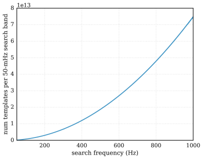
Figure 1: For this search, the number of templates per 50-mHz search band increases quadratically with $f$. At each value of $f$, the ${\dot{f}}$ search range is [-$f/\tau_{\textrm{NS}}$, 0] and the $\ddot{f}$ search range is [0, $2f/\tau_{\textrm{NS}}^{2}$]. In total, $4.99\times 10^{17}$ templates are included in this search.

We perform a semi-coherent search and rank the results according to the line-robust statistic $\widehat{O}_{{{\mathrm{{S}}}{\mathrm{{G}}{\mathrm{{L}}}}}}$ Keitel et al. (2014), in a manner similar to Abbott et al. (2016); Singh et al. (2016). The basic ingredient is the averaged $\mathcal{F}$ statistic Jaranowski et al. (1998); Cutler and Schutz (2005), $\overline{\mathcal{F}}$, computed using the Global Correlation Transform (GCT) method Pletsch and Allen (2009); Pletsch (2012). In a stack-slide search, the time series data are partitioned into $i=1...{N_{\mathrm{seg}}}$ segments of length $T_{\mathrm{coh}}$ each. The data from every segment are match-filtered against a set of signal templates each specified by a set of parameters (the signal frequency $f$, the first-order spindown ${\dot{f}}$, the second-order spindown $\ddot{f}$, and the sky position) to produce values of the detection statistic $\mathcal{F}_{i}$ for each segment (the coherent step). These $\mathcal{F}_{i}$ values are then combined to produce an average value of the statistic across the ${N_{\mathrm{seg}}}$ segments, $2\overline{\mathcal{F}}$, which is the core statistic that we use in these analyses (the incoherent step). The values of the signal template parameters $f$, ${\dot{f}}$, and $\ddot{f}$ are given by a predetermined grid. The $f$ grid spacing (i.e., the separation between two adjacent values of $f$ in the search) is kept the same for the coherent and incoherent steps, while the spacings for the ${\dot{f}}$ and $\ddot{f}$ grids for the incoherent summing are finer by factors of 90 and 60, respectively. The search parameters are summarized in Table 1 and were derived using the optimisation scheme described in Prix and Shaltev (2012) assuming a run duration of 6 months on Einstein@Home.

II.3 The detection and ranking statistics

The 2$\overline{\mathcal{F}}$ statistic gives a measure of the likelihood that the data resembles a signal versus Gaussian noise; therefore, signals are expected to have high values of $2\overline{\mathcal{F}}$. However, line disturbances in the data can also result in high values of $2\overline{\mathcal{F}}$. The line-robust statistic, $\widehat{O}_{{{\mathrm{{S}}}{\mathrm{{G}}{\mathrm{{L}}}}}}$, was designed to address this by testing the signal hypothesis against a composite noise model comprising a combination of Gaussian noise and a single-detector spectral line. The $\widehat{O}_{{{\mathrm{{S}}}{\mathrm{{G}}{\mathrm{{L}}}}}}$ parameters are tuned as described in Keitel et al. (2014) using simulations so that the detection efficiency of $\widehat{O}_{{{\mathrm{{S}}}{\mathrm{{G}}{\mathrm{{L}}}}}}$ performs as well as $2\overline{\mathcal{F}}$ in Gaussian noise and better in the presence of lines. For this search, the value of $c^{\star}$ (related to the tuning parameter in the choice of prior, see Keitel et al. (2014)) is set to be $34.8$, which corresponds to a Gaussian false-alarm probability of $10^{-9}$.

The $\widehat{O}_{{{\mathrm{{S}}}{\mathrm{{G}}{\mathrm{{L}}}}}}$ distribution even in Gaussian noise is not known analytically. Therefore, although we use the $\widehat{O}_{{{\mathrm{{S}}}{\mathrm{{G}}{\mathrm{{L}}}}}}$ toplists to find the best signal candidates, we still use $2\overline{\mathcal{F}}$ as the detection statistic for ascertaining a candidate’s significance. For a stack-slide search with ${N_{\mathrm{seg}}}$ segments, the ${N_{\mathrm{seg}}}\times 2\overline{\mathcal{F}}$ distribution in Gaussian noise follows a chi-squared distribution with $4{N_{\mathrm{seg}}}$ degrees of freedom Wette (2012).

II.4 The parameter space

Since the spin parameters of Cas A are unknown, our search encompasses a large range of possible gravitational-wave frequencies $f$; namely, from 50 to 1000 Hz. For a given value of $f$, the ${\dot{f}}$ and $\ddot{f}$ ranges are given by the following specifications:

$${\dot{f}} \in[-f/\tau_{\mathrm{NS}},0]$$ (1)

$$\ddot{f} \in[0,2f/\tau_{\mathrm{NS}}^{2}]$$ (2)

where $\tau_{\mathrm{NS}}$ is the fiducial age of the neutron star, taken to be 300 years. As discussed in Abadie et al. (2010), this choice of $\tau_{\mathrm{NS}}$ is on the young end of the age estimates, which yields a larger search parameter space than other, less conservative choices. The searched parameter space at each value of $f$ is a rectangle in the ${\dot{f}}-\ddot{f}$ plane, and the search volume increases quadratically with $f$ (Fig. 1).

Compared to Wette et al. (2008); Abadie et al. (2010); Aasi et al. (2015), the largest magnitude of the first order spindown parameter is the same, corresponding to a conservative assumption (in the sense that it allows for the broadest range of first order spindown values) on the average braking index at fixed age of the object. The range of the second order spindown is constructed differently here than in Abadie et al. (2010); Aasi et al. (2015) in that it does not depend on ${\dot{f}}$. The highest searched value of $\ddot{f}$ is $n{{{{\dot{f}}^{2}}_{\textrm{max}}}/f}$, with $n=2$ being the instantaneous braking index. The searches mentioned above took this as the lower boundary of the $\ddot{f}$ range and set the upper boundary at $n=7$. Our choice does not search such a broad range of $\ddot{f}$ values, and is driven by ease of set-up of the search. Observational data on braking indexes supports this choice Hamil et al. (2015).

We estimate that searching over third order spindown values is not necessary. We do this by counting how many templates are needed to cover the third order spindown range. The 3rd order spindown template extent ${\Delta\dddot{f}}$ in a semi-coherent search with mismatch $m$ is

$${\Delta}\dddot{f}={1\over\gamma_{3}}{{2520\sqrt{m}}\over{\pi T_{\textrm{\mbox{\tiny{coh}}}}^{4}}}.$$ (3)

For this search we set $m=0.2$ and $\gamma_{3}\simeq 3.89\times 10^{5}$ Shaltev (2012). The template extent of Eq. 3 is $\sqrt{mg^{33}}$ where $g^{ij}$ is the inverse of the phase metric Wette (2015). The 3rd order spindown range, consistent with the choices of Eq. 2, is $6{f/\tau_{\textrm{NS}}^{3}}$. With $\tau_{\mathrm{NS}}=300$ years, we find that we do not need more than a single template to cover the 3rd order spindown range; therefore, we do not need to add a 3rd order spindown dimension.

The location of Cas A is known to within $\sim$ 1”, which is smaller than the sky resolution of our search. Hence, we only search a single sky position (right ascension = 23h 23m 28s, declination = 58^∘ 58’ 43”).

II.5 Distribution of the computational load

The search runs on volunteer computers in the Einstein@Home network, and is split into 9.2 million work units (WUs), with each WU designed to run for about six hours on a modern PC. A single WU encompasses a 50-mHz range in $f$ and the entire range of $\ddot{f}$ at the start value of $f$, along a single slice out of the ${\dot{f}}$ range. The results from WUs that search over the same 50-mHz range are combined into a single band, and these multiple WUs together cover the entire ${\dot{f}}$ range at that value of $f$. Each WU searches through approximately $5\times 10^{10}$ templates, and returns two lists of results corresponding to the 3000 templates with the highest values of the 2$\mathcal{F}$ and $\widehat{O}_{{{\mathrm{{S}}}{\mathrm{{G}}{\mathrm{{L}}}}}}$ statistics (described in section II.3), called the toplists. The total number of templates included in this search is $4.99\times 10^{17}$.

II.6 Semiautomatic identification of disturbances

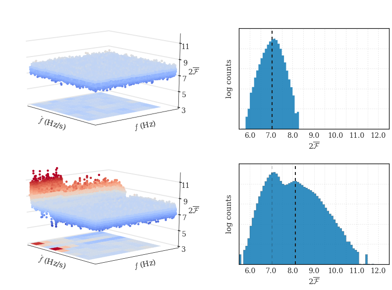
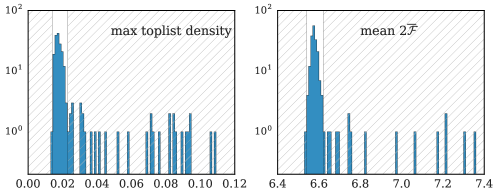
Figure 2: The maximum density (left) and the mean $2\overline{\mathcal{F}}$ value (right) for the candidates are the two metrics we use to identify potentially disturbed bands. Left: undisturbed bands (an example in the top panels) have a very uniform density of candidates in $f$-${\dot{f}}$, while disturbed bands (an example in the bottom panels) present marked overdensities. The $2\overline{\mathcal{F}}$ values in $f$-${\dot{f}}$ plane are shown in the 3D plot, while the candidate density is shown in the 2D projections.The maximum density in a disturbed band tends to be much higher (here, more red) than the maximum density in an undisturbed band. Right: The $2\overline{\mathcal{F}}$ distribution in an undisturbed band (top) and in a disturbed band (bottom).

Figure 3: The distributions of maximum toplist density (left) and mean toplist $2\overline{\mathcal{F}}$ (right) are shown for a sample 10-Hz frequency range. Both distributions consist of an undisturbed body with a disturbed tail (hatched). All 50-mHz bands that fall within the hatched areas are marked as potentially disturbed.

When the noise is purely Gaussian, the 2$\overline{\mathcal{F}}$ distribution is well-modelled and the significances of signal candidates can be determined in a straight-forward manner. However, disturbances generate deviations from the expected distribution. In order to meaningfully use the same statistical analysis on all of the candidates, the disturbed 50-mHz bands must be excluded from the search. Previous searches Singh et al. (2016); Abbott et al. (2016) relied on a visual inspection of the full data set in order to identify the disturbed bands, which is a very time consuming endeavor. Here, we introduce a semiautomatic method that greatly reduces the number of bands that need to be visually inspected.

We use two indices to identify bands that cannot automatically be classified as undisturbed: 1) the density of toplist candidates in that band and 2) their average $2\overline{\mathcal{F}}$. We classify as undisturbed those bands whose maximum density and average $2\overline{\mathcal{F}}$ are well within the bulk distribution of the values for these quantities in the neighbouring frequency bands, and mark the remainder as potentially disturbed and in need of visual inspection.

The size of the toplist and the frequency grid spacing are fixed. Therefore, when a disturbance is present in a 50-mHz band, the toplists within that band disproportionately include templates in the parameter space near the disturbance. We look for evidence of disturbances in the 50-mHz bands using a method that mimics and replaces the visual inspection used in previous searches Abbott et al. (2016): For a given band, we calculate the density of candidates in a $10\times 10$ grid in $f$-${\dot{f}}$ space, and take the maximum density as an indicator of how disturbed the band is likely to be. Since disturbances also manifest as deviations in the $2\overline{\mathcal{F}}$ distribution, we use the mean of $2\overline{\mathcal{F}}$ as an additional indicator of how much a band is disturbed. A visual representation of these concepts is shown in Fig. 3.

Because the search volume increases with $f$, both the mean of $2\overline{\mathcal{F}}$ and the candidate density vary with frequency. To account for this effect, we compare the observed maximum density and mean $2\overline{\mathcal{F}}$ from each band with the distribution of maximum density and mean $2\overline{\mathcal{F}}$ values in sets of 200 contiguous 50-mHz bands (10 Hz). These constitute our reference distributions.

Since the majority of bands are undisturbed, the reference distributions are composed of a well-defined bulk (from the undisturbed bands) with tails (disturbed bands), as illustrated in Fig. 3. We define the “bulk” of each distribution by eye, and then mark the bands that fall outside of this bulk on either side as being potentially disturbed; we generally expect disturbed bands to be in the upper ends of the distributions (that is, to have particularly large values of maximum density and mean $2\overline{\mathcal{F}}$) but also include bands in the lower ends so as not to miss any unexpected disturbed behavior. We proceed with a full visual inspection only of this potentially disturbed subset. Fig. 3 shows the reference distributions for the bands between 90 and 100 Hz. These are typical examples and illustrate how the “by eye” definition of the bulk of the distributions is not subtle. When selecting the bulk, we err on being conservative: when in doubt, we label bands as being potentially disturbed, as these will be re-inspected later.

If a signal were present, it would not be excluded because of the automated procedure. On the one hand, if it were so weak that the band would not be marked as disturbed, the band would automatically be included in the analysis. On the other hand, if it were strong enough that the automated procedure mark its band as being potentially disturbed, then it would be visually inspected by a human who would recognise the signature of a signal and not discard the band.

This method still requires human input in two steps: first, to define the bulk of the reference distributions; and second, to inspect the subset of potentially disturbed bands. However, the “calibration” work necessary for determining the bulk of the reference distributions only requires the inspection of 2 distributions every 10 Hz rather than multiple distributions every 50 mHz. Furthermore, the bands that do not pass the undisturbed-classification criteria and require visual inspection are only 15% of the total set. Overall, this procedure still cuts down the required time from multiple days with multiple people to a few hours by a single person.

This procedure requires minimal tuning and relies only on the assumption that the reference distributions are predominantly undisturbed. This has so far been our experience on all the LIGO data sets that we have inspected. We are confident that this method can be applied to other sets of gravitational wave data.

When we compare this method against a full visual inspection of a few search frequency ranges (50 to 100 Hz, 450 to 500 Hz, and 950 to 1000 Hz), it identifies $\sim\!95\%$ of the disturbed bands and misses only the most marginal disturbances. After we apply this method to the entire frequency range, we exclude a total of 1991 50-mHz bands as being disturbed ($\sim\!10\%$); these are listed in Table S2.

II.7 Analysis of undisturbed bands

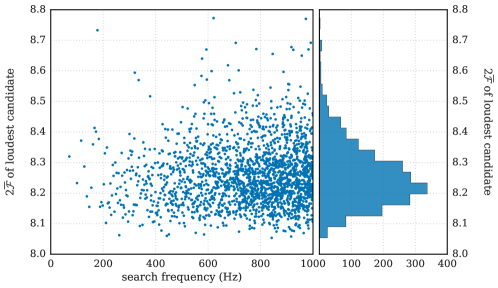
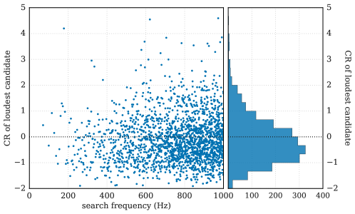
Figure 4: For each of the 2000 partitions, we determine the $2\overline{\mathcal{F}}$ of the loudest candidates (top) as well as their CR values (bottom), where CR is defined in Eq. 4.

The $2\overline{\mathcal{F}}$ distribution in Gaussian noise only depends on the number of effectively independent templates searched ($N$). However, the grid spacings are chosen to maximize signal recovery, so the $N$ templates are not fully independent. The observed distribution is instead described by an effective number of templates $N_{\mathrm{eff}}<N$. The value of $N_{\mathrm{eff}}$ is obtained by fitting the distribution of the loudest candidates (i.e., the highest values of $2\overline{\mathcal{F}}$).

We divide the entire set of 50-mHz bands across our search frequency range into 2000 partitions of approximately equal parameter space volume, which results in $\sim\!2\times 10^{14}$ templates per partition. In order to create these partitions, we calculate an exact partitioning of the total search volume and divide the full range of 50-mHz bands so that the number of templates in each partition best matches the number of templates in the exact partitioning. Since the number of templates in a band grows with frequency, the frequency width spanned by each partition decreases with increasing frequency. This can be clearly seen in the left panels of Fig. 4. In this way, since each partition contains roughly the same number of search templates, the expected loudest candidate in each partition is the same and drawn from the same underlying distribution, defined by $N_{\mathrm{eff}}$. For this search, we find that $N_{\mathrm{eff}}/N~{}\approx~{}0.65$.

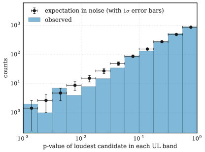
Figure 5: The p-values for the loudest candidate in each UL band is plotted in the blue histogram, and the expectation in Gaussian noise is shown in the black scatter points. We do not find any excess in our search. The small systematic deviation in our data from the expected is caused by a subtle difference in the $\widehat{O}_{{{\mathrm{{S}}}{\mathrm{{G}}{\mathrm{{L}}}}}}$- and $2\overline{\mathcal{F}}$- rankings.

Fig. 4 shows both the $2\overline{\mathcal{F}}$ (top) and the critical ratio CR (bottom) for the loudest candidates. We define CR as

$$CR:=\frac{2\overline{\mathcal{F}}_{\mathrm{meas}}-2\overline{\mathcal{F}}_{\mathrm{exp}}}{\sigma_{2\overline{\mathcal{F}}}}$$ (4)

where $2\overline{\mathcal{F}}_{\mathrm{meas}}$ is the measured value of the loudest, $2\overline{\mathcal{F}}_{\mathrm{exp}}$ the expected value of the loudest, and $\sigma_{2\overline{\mathcal{F}}}$ is the expected standard deviation for the loudest over a partition. The loudest candidate over the entire search is in the 620.85 Hz band and has a $2\overline{\mathcal{F}}$ value of 8.77; this is also the most significant candidate, with a CR of 4.56. However, if we consider the entire searched parameter space rather than just the partition at 620.85 Hz, the CR value of the most significant candidate drops to $<0$; i.e., the expected loudest is actually higher than the loudest that we observe. This tells us that our search has not revealed any gravitational wave signal from Cas A in the targeted waveform parameter space, as even the template that most resembles a signal has a statistical significance that is well within the expectations due to random chance.

We convert the CR values of the loudest candidates to p-values to represent the chance probability of finding a partition-loudest candidate as significant as or more significant than what was measured in the search. The results are plotted in Fig. 5, along with the expected distribution of p-values in Gaussian noise. There is a small systematic deviation from the expected distribution which arises from a subtle difference between the $\widehat{O}_{{{\mathrm{{S}}}{\mathrm{{G}}{\mathrm{{L}}}}}}$ and $2\overline{\mathcal{F}}$ toplists and is not due to any physical effect.

III Upper limits

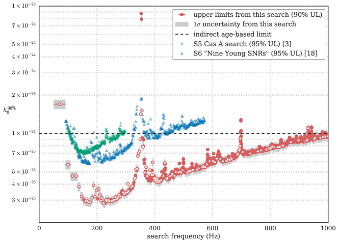
Figure 6: $90\%$ confidence strain amplitude upper limits in each of the 2000 partitions. The results for partitions that contain only undisturbed 50-mHz bands are plotted in the filled red circles, while the results for partitions with disturbed 50-mHz bands are plotted in the open red circles. We also plot the 95% confidence upper limits from two previous searches on Cas A in green and blue. Our upper limits beat the so-called indirect age-based limit Wette et al. (2008) across the band.

We find no candidates with $CR>5$ and no excess in the p-value distribution. Therefore, we set frequentist 90% upper limits on the continuous gravitational-wave strain $h_{0}^{90\%}$ in our search range using the process described in previous works Abbott et al. (2016); Singh et al. (2016), which we summarise below.

The $h_{0}^{90\%}$ in a partition is the gravitational-wave amplitude at which 90% of a population of signals with parameters within the partition would produce a more significant candidate than the most significant candidate measured by the search in that partition. We determine $h_{0}^{90\%}$ by injecting signals at fixed amplitudes bracketing the $h_{0}^{90\%}$ level, then running the search on these injections and counting how many injections were recovered (i.e., how many produced a candidate more significant than the loudest measured by the actual search). Because this injection-and-recovery procedure is time-consuming, we perform it on only a subset of twenty representative partitions — uniformly distributed in frequency in the search range — rather than the full set of 2000, and use these results to derive the upper limits in all the other partitions.

For each of the twenty injection partitions, we fit a sigmoid to the detection efficiency (the fraction of recovered injections) as a function of injection amplitude to determine both the value of $h_{0}^{90\%}$ and the 1-$\sigma$ uncertainty on $h_{0}^{90\%}$. We determine the $h_{0,\textrm{CR}_{i}}^{90\%,j}$ in each of the injection partitions corresponding to different detection criteria binned by CR, with $\textrm{CR}_{i}=[0,~{}1,~{}2,~{}3,~{}4,~{}5]$. For each $\textrm{CR}_{i}$, we derive the corresponding sensitivity depths

$${\mathcal{D}}_{\textrm{CR}_{i}}^{90\%,j}={{\sqrt{S_{h}(f_{j})}}\over{h_{0,\textrm{CR}_{i}}^{90\%,j}}}~{}~{}~{}[1/\sqrt{\text{Hz}}].$$ (5)

By design, the sensitivity depths of this search are roughly constant across the different partitions. We estimate the sensitivity depths by averaging the values across the injection partitions:

$${\mathcal{D}}_{\textrm{CR}_{i}}^{90\%}={1\over 20}\sum_{j=1}^{20}{\mathcal{D}}_{\textrm{CR}_{i}}^{90\%,j}.$$ (6)

For each of the remaining partitions, at frequencies around $f_{k}$, we derive the upper limit as

$${h{{}_{0}^{90\%}}(f_{k})}={{\sqrt{S_{h}(f_{k})}}\over{{{\mathcal{D}}}_{\textrm{CR}_{i}(f_{k})}^{90\%}}},$$ (7)

where $\textrm{CR}_{i}(f_{k})$ is the significance bin of the loudest candidate of the partition at $f_{k}$ and $S_{h}(f_{k})$ the power spectral density of the data. ${\mathcal{D}}_{\textrm{CR}_{i}}^{90\%}\simeq 70$ Hz^-1/2 for this search.

Our upper limits are plotted in Fig. 6 in red with 1-$\sigma$ uncertainties in gray, and provided in tabular form as Supplemental Material. The uncertainties in $h_{0}^{90\%}$ that we report here are propagated from the statistical uncertainties in fitting the recovery. The partitions containing disturbed bands (which were not included in the analysis) are marked with open circles.

The upper limit value near 170 Hz, where the detectors are the most sensitive, is $2.9\times 10^{-25}$. This value is roughly two times lower than the previous most constraining upper limit on Cas A Aasi et al. (2015), plotted in blue, which also used S6 data. Our upper limits are also more than twice as constraining as an earlier Cas A search, plotted in green Abadie et al. (2010), which ran on S5 data. Our upper limits beat the so-called indirect age-based limit Wette et al. (2008) across the vast majority of the frequency range.

IV Conclusions

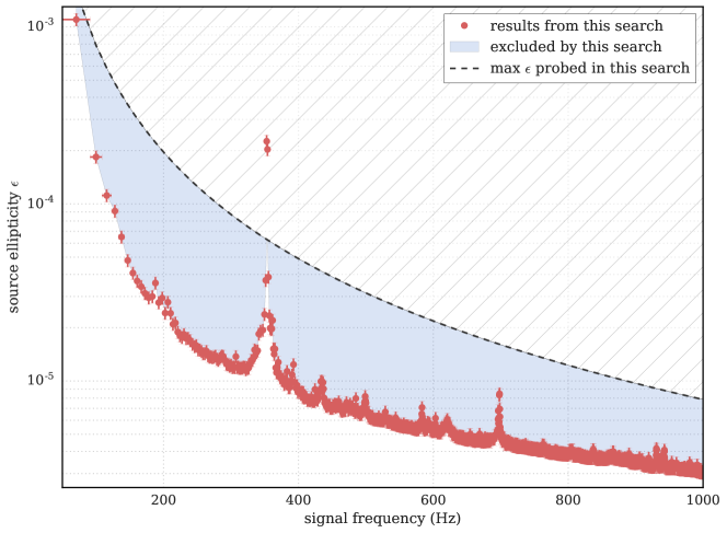
Figure 7: With a few reasonable assumptions, we can convert the upper limits on the gravitational-wave strain to upper limits on the ellipticity of Cas A. The shaded area denotes the source ellipticities (as a function of signal frequency) that are excluded by this search: ellipticities in this region would have produced signals that this search would have detected. The dashed line marks the spindown ellipticity probed by this search and is set by our choice of $\dot{f}$ search range.

The upper limits on the gravitational wave strain from Cas A translate into constraints on the shape of Cas A. As described in Ming et al. (2016), a neutron star’s mass distribution can be described by the ellipticity $\epsilon$, where

$$\epsilon=\frac{\left|I_{xx}-I_{yy}\right|}{I_{zz}}$$ (8)

and $I_{zz}$ is the principal moment of inertia of the star around its rotational axis. If a neutron star at a distance $D$ and spinning at a frequency $f/2$ has a non-axisymmetric distortion $\epsilon$, then it will produce a continuous gravitational wave with a frequency $f$ and amplitude $h_{0}$. These quantities are related to each other as follows:

$$\epsilon=\frac{h_{0}D}{f^{2}}\frac{c^{4}}{4\pi^{2}I_{zz}G}.$$ (9)

Eq. 9 shows how we can re-express the constraints on the gravitational wave amplitude as constraints on the ellipticity. We take the distance to Cas A to be 3.4 kpc Fesen et al. (2006) and $I_{zz}$ to be $10^{38}$ kg m².

These constraints on source ellipticity are shown in Fig. 7. For instance, if Cas A is emitting gravitational waves at around 200 Hz (and, therefore, spinning at a frequency of 100 Hz), its ellipticity should be less than a few times $10^{-5}$, since we would have been able to detect gravitational waves produced by larger ellipticities.

The maximum ellipticity is the ellipticity necessary to sustain emission at the spindown limit, i.e., when all of the lost rotational energy is radiated as gravitational waves. This spindown ellipticity is

$$\epsilon^{sd}=\sqrt{\frac{5c^{5}}{32\pi^{4}G}\frac{x|\dot{f}|}{If^{5}}}~{}~{}\textrm{with~{} x=1},$$ (10)

where ${\dot{f}}$ is twice the spin-frequency derivative.

The highest spin-down ellipticity for an object emitting gravitational waves at a frequency $f$ that our search could have detected can be computed from Eq. 10 by setting ${\dot{f}}=f/300$ years. For an isolated system, if ${\dot{f}}$ is twice the spin-frequency derivative, larger ellipticities would violate energy conservation. For this reason we only highlight the region between the ellipticity upper limit curve and the spindown ellipticity curve as excluded by the search. However, we note that systems in general could have ellipticities larger than the spindown ellipticity if the gravitational wave ${\dot{f}}$ (the apparent ${\dot{f}}$) differs from the intrinsic one due to, for example, radial motion.

V Acknowledgments

The authors thank the Einstein@Home volunteers who have supported this work by donating compute cycles of their machines. Maria Alessandra Papa, Bruce Allen and Xavier Siemens gratefully acknowledge the support from $\mathrm{NSF\;PHY}$ Grant 1104902. All the post-processing computational work for this search was carried out on the $\mathrm{ATLAS}$ super-computing cluster at the Max-Planck-Institut für Gravitationsphysik / Leibniz Universität Hannover. We also acknowledge the Continuous Wave Group of the LIGO Scientific Collaboration for useful discussions. This document has been assigned LIGO Laboratory document number LIGO-P1600212.

References

- Fesen et al. (2006) R. A. Fesen et al., “The expansion asymmetry and age of the Cassiopeia A supernova remnant,” Astrophys. J. 645, 283 (2006).
- Ho and Heinke (2009) W. C. G. Ho and C. O. Heinke, “A neutron star with a carbon atmosphere in the Cassiopeia A supernova remnant,” Nature 462, 71 (2009).
- Abadie et al. (2010) J. Abadie et al., “First search for gravitational waves from the youngest known neutron star,” Astrophys. J. 722, 1504 (2010).
- (4) https://www.einsteinathome.org.
- Abbott et al. (2009) B. P. Abbott et al., “LIGO: The Laser Interferometer Gravitational-Wave Observatory,” Rep. Prog. Phys. 72 (2009).
- Abadie et al. (2012) J. Abadie et al., “Sensitivity Achieved by the LIGO and Virgo Gravitational Wave Detectors during LIGO’s Sixth and Virgo’s Second and Third Science Runs,” (2012), arXiv:1203.2674 [hep-th] .
- Shaltev (2016) M. Shaltev, “Optimizing the StackSlide setup and data selection for continuous-gravitational-wave searches in realistic detector data,” Phys. Rev. D 93, 044058 (2016).
- Abbott et al. (2016) B. P. Abbott et al., “Results of the deepest all-sky survey for continuous gravitational waves on LIGO S6 data running on the Einstein@Home volunteer distributed computing project,” submitted to Phys. Rev. D (2016), arXiv:1606.09619 [gr-qc] .
- Singh et al. (2016) A. Singh et al., “Results from an all-sky high-frequency Einstein@Home search for continuous gravitational waves in the LIGO 5th Science Run,” Phys. Rev. D 94, 064061 (2016).
- Keitel et al. (2014) D. Keitel et al., “Search for continuous gravitational waves: Improving robustness versus instrument artifacts,” Phys. Rev. D 89, 060423 (2014).
- Jaranowski et al. (1998) P. Jaranowski, A. Królak, and B. F. Schutz, “Data analysis of gravitational-wave signals from spinning neutron stars: The signal and its detection,” Phys. Rev. D 58, 063001 (1998).
- Cutler and Schutz (2005) C. Cutler and B. F. Schutz, “Generalized -statistic: Multiple detectors and multiple gravitational wave pulsars,” Phys. Rev. D 72, 063006 (2005).
- Pletsch and Allen (2009) H. J. Pletsch and B. Allen, “Exploiting Large-Scale Correlations to Detect Continuous Gravitational Waves,” Phys. Rev. Letters 103, 181102 (2009).
- Pletsch (2012) H. J. Pletsch, “Parameter-space metric of semicoherent searches for continuous gravitational waves,” Phys. Rev. D 82, 042002 (2012).
- Prix and Shaltev (2012) Reinhard Prix and Miroslav Shaltev, “Search for Continuous Gravitational Waves: Optimal StackSlide method at fixed computing cost,” Phys. Rev. D 85, 084010 (2012).
- Wette (2012) K. Wette, “Estimating the sensitivity of wide-parameter-space searches for gravitational-wave pulsars,” Phys. Rev. D 85, 042003 (2012).
- Wette et al. (2008) K. Wette et al., “Searching for gravitational waves from Cassiopeia A with LIGO,” Class. Quant. Grav. 25, 235011 (2008).
- Aasi et al. (2015) J. Aasi et al., “Searches for continuous gravitational waves from nine young supernova remnants,” Astrophys. J. 813, 1 (2015).
- Hamil et al. (2015) O. Hamil, J. R. Stone, M. Urbanec, and G. Urbancová, “Braking index of isolated pulsars,” Phys. Rev. D 91, 063007 (2015).
- Shaltev (2012) Miroslav Shaltev, “Coherent follow-up of continuous gravitational-wave candidates: minimal required observation time,” Journal of Physics: Conference Series 363, 012043 (2012).
- Wette (2015) Karl Wette, “Parameter-space metric for all-sky semicoherent searches for gravitational-wave pulsars,” Phys. Rev. D 92, 082003 (2015).
- Papa et al. (2016) M. A. Papa et al., “Hierarchical follow-up of sub-threshold candidates of an all-sky Einstein@home search for continuous gravitational waves on LIGO data,” submitted to Phys. Rev. D (2016), arXiv:1608.08928 [astro-ph] .
- Ming et al. (2016) J. Ming et al., “Optimal directed searches for continuous gravitational waves,” Phys. Rev. D. 93, 064011 (2016).