The Vev Flip-Flop: Dark Matter Decay between Weak Scale Phase Transitions

Abstract

We propose a new alternative to the Weakly Interacting Massive Particle (WIMP) paradigm for dark matter. Rather than being determined by thermal freeze-out, the dark matter abundance in this scenario is set by dark matter decay, which is allowed for a limited amount of time just before the electroweak phase transition. More specifically, we consider fermionic singlet dark matter particles coupled weakly to a scalar mediator $S_{3}$ and to auxiliary dark sector fields, charged under the Standard Model gauge groups. Dark matter freezes out while still relativistic, so its abundance is initially very large. As the Universe cools down, the scalar mediator develops a vacuum expectation value (vev), which breaks the symmetry that stabilises dark matter. This allows dark matter to mix with charged fermions and decay. During this epoch, the dark matter abundance is reduced to give the value observed today. Later, the SM Higgs field also develops a vev, which feeds back into the $S_{3}$ potential and restores the dark sector symmetry. In a concrete model we show that this “vev flip-flop” scenario is phenomenologically successful in the most interesting regions of its parameter space. We also comment on detection prospects at the LHC and elsewhere.

The WIMP (Weakly Interacting Massive Particle) paradigm in dark matter physics states that dark matter (DM) particles should have non-negligible couplings to Standard Model (SM) particles. Their abundance today would then be determined by their abundance at freeze-out, the time when the temperature of the Universe dropped to the level where interactions producing and annihilating DM particles become inefficient. In many models these interactions should still be observable today, through residual DM annihilation in galaxies and galaxy clusters, through scattering of DM particles on atomic nuclei, or through DM production at colliders. The conspicuous absence of any convincing signals [1, 2, 3, 4, 5, 6, 7] to date motivates us to look for alternatives to the WIMP paradigm.

In this letter, we present a scenario in which the DM abundance is set not by annihilation, but by decay. We focus on models in which fermionic DM particles couple to a new scalar species and argue that the resulting scalar potential may undergo multiple phase transitions, “flip-flopping” between phases in which the symmetry stabilising the DM is intact and a phase where it is broken. Similar behaviour is found in models of electroweak baryogenesis [8, 9, 10, 11, 12, 13, 14], see also [15] for related work. During the broken phase, the initially overabundant DM particles are depleted until their relic density reaches the value observed today. Although the resulting picture of early freeze out, followed by a period of DM decay around the weak scale, is quite generic, we focus here on a concrete example and comment on possible generalisations in the end.

Field	Spin	SM	$\mathbb{Z}_{3}$	mass scale
$\chi$	$\tfrac{1}{2}$	$(1,1,0)$	$\chi\to e^{2\pi i/3}\chi$	TeV
$S_{3}$	$0$	$(1,3,0)$	$S_{3}\to e^{2\pi i/3}S_{3}$	100 GeV
$\Psi_{3}$	$\tfrac{1}{2}$	$(1,3,0)$	$\Psi_{3}\to e^{-2\pi i/3}\Psi_{3}$	TeV
$\Psi_{3}^{\prime}$	$\tfrac{1}{2}$	$(1,3,0)$	$\Psi_{3}^{\prime}\to e^{-2\pi i/3}\Psi_{3}^{\prime}$	TeV

Table 1: New particles in our toy model, with their mass scales and charge assignments under the SM gauge group $SU(3)_{c}\times SU(2)_{L}\times U(1)_{Y}$ and under the dark sector $\mathbb{Z}_{3}$ symmetry.

Model Framework.—We introduce a complex dark sector scalar $S_{3}$ that is a triplet under the SM $SU(2)_{L}$ gauge symmetry and carries zero hypercharge. We take the DM particle to be a multi-TeV Dirac fermion $\chi$, uncharged under the SM gauge group. To offer the DM particle a decay mode, we also introduce two multi-TeV Dirac fermion triplets $\Psi_{3}=(\psi^{+},\psi^{0},\psi^{-})$ and $\Psi_{3}^{\prime}=(\psi^{\prime+},\psi^{\prime 0},\psi^{\prime-})$. All new particles are charged under a symmetry that stabilises the dark sector and is taken here as a $\mathbb{Z}_{3}$, which could be a remnant of a dark sector gauge symmetry broken at a scale $\gg\text{TeV}$. The dark sector particle content is summarised in table 1.

The tree level scalar potential and the relevant Yukawa terms in the Lagrangian of the model are

$$\mathcal{L}_{\text{scalar}} =\mu_{H}^{2}H^{\dagger}H-\lambda_{H}(H^{\dagger}H)^{2}$$

$$+\mu_{S}^{2}S_{3}^{\dagger}S_{3}-\lambda_{S}(S_{3}^{\dagger}S_{3})^{2}-\lambda_{3}(S_{3}^{\dagger}T^{a}S_{3})^{\dagger}(S_{3}^{\dagger}T^{a}S_{3})$$

$$-\alpha(H^{\dagger}H)(S_{3}^{\dagger}S_{3})-\beta(H^{\dagger}\tau^{a}H)(S_{3}^{\dagger}T^{a}S_{3})\,,$$ (1)

$$\mathcal{L}_{\text{Yuk}} =y_{\chi}S_{3}^{\dagger}\bar{\chi}\Psi_{3}+y_{\chi}^{\prime}S_{3}^{\dagger}\bar{\chi}\Psi_{3}^{\prime}+y_{\Psi}\epsilon^{ijk}S_{3}^{i}\overline{\Psi_{3}^{j}}(\Psi_{3}^{\prime k})^{c}+h.c.$$ (2)

The first line in eq. 1 contains the SM Higgs potential, characterised by the tree-level mass parameter $\mu_{H}\simeq 88$ GeV and the quartic coupling $\lambda_{H}\simeq 0.12$. We will use $H=(G^{+},(h+iG^{0})/\sqrt{2})$. In the second line, the analogous potential for the scalar mediator $S_{3}=(s^{+},(s+ia)/\sqrt{2},s^{-})$ is given. It is characterised by $\mu_{S}\sim\mathcal{O}(\text{100\leavevmode\nobreak\ GeV})$ and positive quartic couplings $\lambda_{S},\lambda_{3}\sim\mathcal{O}(1)$. We will use the convention that only the electrically neutral, CP even components $h$ and $s$ of $H$ and $S_{3}$ acquire vevs. The third line of eq. 1 contains the Higgs portal terms with couplings $\alpha$ and $\beta$. The symmetries of the model are designed to allow new Yukawa couplings involving $S_{3}$, $\chi$, $\Psi_{3}$ and $\Psi_{3}^{\prime}$ with small coupling constants $y_{\chi}$, $y_{\chi}^{\prime}$. When ${\langle s\rangle}\neq 0$, these couplings will lead to mixing between $\chi$, $\Psi_{3}$ and $\Psi_{3}^{\prime}$ and thus to DM decay via $\chi\to W\Psi_{3}$, $\chi\to W\Psi_{3}^{\prime}$. The masses $m_{\chi}$, $m_{\Psi}$, $m_{\Psi^{\prime}}$ of the new fermions are assumed to be such that the decay channels $\chi\to S_{3}\Psi_{3}$, $\chi\to S_{3}\Psi_{3}^{\prime}$ are forbidden today. If these decay channels were open, the DM candidates would be $\psi^{0}$, $\psi^{\prime 0}$ and $S$ instead of $\chi$, and their abundance would be determined by a regular thermal freeze-out. DM decays to $S\Psi_{3}$ and $S\Psi_{3}^{\prime}$ may still be open at early times as the masses of $S_{3}$, $\Psi_{3}$, and $\Psi_{3}^{\prime}$ are $T$-dependent. In particular, when ${\langle s\rangle}\neq 0$, the coupling $y_{\Psi}\sim\mathcal{O}(1)$ in the last line of eq. 2 leads to mass shifts for $\psi^{\pm}$ and $\psi^{\prime\pm}$. The same term also allows $\Psi_{3}$ and $\Psi_{3}^{\prime}$ to annihilate efficiently into SM particles.

We assume that the parameters of the scalar potential are chosen such that, at zero temperature, the SM Higgs field has its usual vev ${\langle h\rangle}\equiv v=246$ GeV, while ${\langle s\rangle}=0$. Thus, the electroweak symmetry is broken at temperature $T=0$, while the $\mathbb{Z}_{3}$ symmetry that stabilises DM is unbroken. The tree level masses of the physical Higgs boson $h$ and of $s$ today are given by $m_{h}^{2}=2\mu_{H}^{2}$ and $m_{s}^{2}=-\mu_{S}^{2}+\alpha\mu_{H}^{2}/(2\lambda_{H})$.

The Vev Flip-Flop.—To determine the evolution of the system given by eq. 2 in the hot early Universe, we consider the effective potential $V^{\text{eff}}$. In addition to $V^{\text{tree}}$, the effective potential includes the $T$-independent one-loop Coleman–Weinberg contributions [16], the one-loop $T$-dependent corrections [17], and the resummed higher-order “daisy” contributions [18, 19, 20, 21], see appendix A for details. We include the dominant contributions to these higher order terms from $t,B^{\mu},Z^{\mu},W^{\mu},H$ and $S_{3}$. The Coleman–Weinberg contribution introduces a renormalisation scale, which we set equal to the SM Higgs vev. Note that at high temperature $\mu_{S}^{2}$ receives negative corrections from the one-loop $T$ dependent term, and positive corrections from the “daisy” terms. This means that at high $T$, the $\mathbb{Z}_{3}$ symmetry may be broken or unbroken, depending on which contribution dominates. The SM Higgs vev is always zero at high $T$ for the experimentally determined values of $\mu_{H}^{2}$ and $\lambda_{H}$.

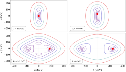
Figure 1: The effective potential $V^{\text{eff}}$ at high $T$ (top left), at the nucleation temperature $T_{S}=385$ GeV where $S_{3}$ obtains a non-zero vev (top right), at the nucleation temperature $T_{n}=143$ GeV where the SM Higgs obtains a vev and the $S_{3}$ vev goes to zero (bottom left), and at $T=0$ (bottom right). Red dots indicate the minima the Universe is in at each stage. Contour lines are evenly spaced on a log scale and range from $1.4\times 10^{6}\text{\,GeV}^{4}$ (purple) to $5.6\times 10^{8}\text{\,GeV}^{4}$ (red), with each contour representing one $e$-fold. For this plot, we have chosen $\alpha=1.33$, $\beta=0$, $\lambda_{S}=\lambda_{3}=1$, and $\mu_{S}^{2}>0$ is fixed such that the tree level mass $m_{s}=185$ GeV at $T=0$ GeV.

We illustrate the main features of the flip-flopping vevs mechanism in fig. 1 for a specific choice of Lagrangian parameters. At high $T$ (top left panel), $V^{\text{eff}}$ is symmetric in both $s$ and $h$. As the Universe cools the $T$-dependent corrections to the $S_{3}$ mass term become subdominant and, since $\mu_{S}^{2}$ is positive, $S_{3}$ develops a non-zero vev at $T=T_{S}$, fig. 1 (top right). Now the $\mathbb{Z}_{3}$ symmetry that stabilises the dark sector is broken, and DM can decay via $\chi\to W\Psi_{3}$ and $\chi\to W\Psi_{3}^{\prime}$. Note that, during this epoch, $SU(2)_{L}$ is also broken and $W^{\mu}$ obtains a mass $m_{W}=g{\langle s\rangle}$, where $g$ is the SM weak gauge coupling. Thanks to the mass shift in $\psi^{\pm}$ and $\psi^{\prime\pm}$, the decay modes $\chi\to S\Psi_{3}$ and $\chi\to S\Psi_{3}^{\prime}$ may also be open.

As the temperature continues to drop $T$-dependent corrections to $\mu_{H}$ become subdominant and $V^{\text{eff}}$ develops new minima at non-zero $\left\langle h\right\rangle$. The extra contribution of this vev to the $S_{3}^{\dagger}S_{3}$ term through the Higgs portal makes the effective $\mu_{S}^{2}$ negative and so ${\langle s\rangle}=0$ is restored at the new minima. At first, the minima at $\left\langle h\right\rangle\neq 0$ are only local minima, but as the temperature drops they become global minima. Typically there is a barrier between the ${\langle s\rangle}\neq 0$ and the ${\langle h\rangle}\neq 0$ minima, so that the phase transition between the two is first order. For the transition to take place, the formation and growth of bubbles of the new phase has to be energetically favourable [22], which happens at $T=T_{n}$, some time after the ${\langle h\rangle}\neq 0$ minima become the global ones. In other words, the Universe is in a supercooled state for some time. To calculate the nucleation temperatures $T_{S}$ and $T_{n}$ we used the publicly available CosmoTransitions package [23, 24, 25, 26]. Note that since the effective potential is gauge dependent away from the minima, the calculated $T_{n}$ may have a residual gauge dependence, see e.g. [27]. As is usual in the baryogenesis literature, we neglect this effect. For our illustrative parameter point, the effective potential at $T_{n}$ is shown in the bottom left panel of fig. 1. At this point the $\mathbb{Z}_{3}$ symmetry is restored and $\chi$ stabilises.

The transition from a phase with unbroken $\mathbb{Z}_{3}$ and $SU(2)_{L}$ at very high $T$ to the broken phase at intermediate $T$, and back to an unbroken phase at the electroweak phase transition is what we call the vev flip-flop. As we approach the present day, $T\sim 0$, the $\left\langle h\right\rangle\neq 0$ minima deepen, and the Universe remains in the phase with broken electroweak symmetry and stable DM, fig. 1 (bottom right).

Dark Matter Abundance.—One of the salient features of the Lagrangian in eq. 2 is that interactions between $\chi$ and the SM always involve the Yukawa couplings $y_{\chi}$, $y_{\chi}^{\prime}$. There is no a priori constraint on the magnitude of these couplings. We focus here on the region of small $y_{\chi},\,y_{\chi}^{\prime}\lesssim 10^{-7}$, where $\chi$ never comes into thermal equilibrium with the SM through the interactions in eq. 2. We thus imagine that a thermal abundance of DM is produced during reheating after inflation or by other new interactions at scales far above the electroweak scale. $\chi$ freezes out when these interactions decouple, at a temperature $T_{\text{fo}}\gg m_{\chi}$. Its abundance at freeze-out is then several orders of magnitude larger than the value observed today, and is independent of $m_{\chi}$, $y_{\chi}$, and $y_{\chi}^{\prime}$. After freeze-out, the DM number density tracks the entropy density until $S_{3}$ develops a vev thanks to the flip-flopping vevs and $\chi$ begins to decay. Recall that during that epoch, $S_{3}$, $\Psi_{3}$, and $\Psi_{3}^{\prime}$ are still in the thermal bath, so processes with these particles in the final state are as good at depleting $\chi$ as processes with only SM particles in the final state would be.

Note that inverse decays like $W\Psi_{3}\to\chi$ are negligible in the parameter space of interest to us as $\chi$ is sufficiently heavy that its abundance is at all times larger than the equilibrium abundance. This would be different at larger values of $y_{\chi}$, $y_{\chi}^{\prime}$, where the interplay of decays and inverse decays would keep $\chi$ in thermal equilibrium until either a conventional thermal freeze-out happens or the electroweak phase transition switches off mixing between $\chi$ and $\Psi_{3}$, $\Psi_{3}^{\prime}$. However, in the parameter region featuring a vev flip-flop, it turns out that neither of these mechanisms can yield the correct DM relic density.

Some time after the $\mathbb{Z}_{3}$ symmetry is restored, the annihilation processes that keep $S_{3}$, $\Psi_{3}$, and $\Psi_{3}^{\prime}$ in thermal equilibrium freeze-out, leaving behind a small, subdominant, relic abundance of $S_{3}$, $\Psi_{3}$, and $\Psi_{3}^{\prime}$. It is crucial in this context that the electrically neutral components of these fields must be lighter than the charged components today to avoid stable charged relics in the Universe. Radiative electroweak corrections indeed lead to a mass splitting of $\mathcal{O}(100\,\text{MeV})$ [28]. For $S_{3}$, we have to make the additional assumption that $\beta\lesssim 0.001$ to avoid a tree level mass splitting that would shift $s^{+}$ ($s^{-}$) downward (upward) by $\tfrac{1}{8}\beta v^{2}/m_{s}$ [29].

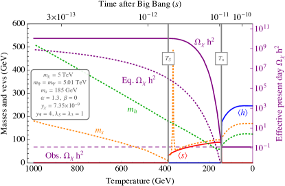
Figure 2: The vev flip-flop: at very high temperatures, both the SM Higgs field vev ${\langle h\rangle}$ (solid blue) and the dark sector scalar vev ${\langle s\rangle}$ (solid red) are zero. As the temperature drops there is a phase transition at $T_{S}$ and $S_{3}$ develops a nonzero vev, breaking the dark sector $\mathbb{Z}_{3}$ symmetry and making the DM unstable. We plot in solid purple the evolution of the effective present day relic density, obtained from the instantaneous DM number density scaled by the subsequent expansion of the Universe. At a lower temperature $T_{n}$, there is a second phase transition where $h$ develops a vev and the feedback of this vev into the dark sector via the Higgs portal restores the $\mathbb{Z}_{3}$ symmetry, halting the DM decay when the observed relic density is reached. The DM equilibrium density (dotted purple), observed relic density (dashed purple), SM Higgs mass $m_{h}$ (dotted green), and $s$ mass $m_{s}$ (dotted orange) are also given.

In fig. 2 we show the evolution of the scalar vevs, the scalar masses and the effective present day DM relic density as the Universe cools, for an illustrative benchmark point with $m_{\chi}=5$ TeV $m_{\Psi}=m_{\Psi^{\prime}}=5.01$ TeV, and $y_{\chi}=y_{\chi}^{\prime}=7.35\times 10^{-9}$. The parameters of the scalar potential are the same as in fig. 1. At the left edge of the plot, at $T=1$ TeV, both scalar fields are without vevs, and the $\chi$ relic density is around eleven orders of magnitude too large. When the temperature reaches $T_{S}\sim 385$ GeV the Universe transitions (via a first order phase transition) to a phase where ${\langle s\rangle}\neq 0$. At this point $\chi$ begins to decay. Most $\chi$ decays happen at temperatures just above the electroweak phase transition as the temperature drops more slowly at later times. At $T\sim 152$ GeV the ${\langle s\rangle}=0$, ${\langle h\rangle}\neq 0$ phase becomes the global minimum, but as there is a barrier in the potential the Universe does not immediately transition to this phase; there is a short period of supercooling until the Universe nucleates to the ${\langle s\rangle}=0$, ${\langle h\rangle}\neq 0$ phase at $T_{n}\sim 143$ GeV with another first order phase transition. At this point the $\mathbb{Z}_{3}$ symmetry is restored and DM decays are no longer possible.

Figure 2 also illustrates that the DM abundance today depends sensitively on the precise value of $T_{n}$ and thus on the parameters of the model. This scenario therefore does not solve the coincidence problem between the observed baryon and DM abundances. On the other hand, if this model is realised in nature, its parameters could be inferred with high precision from cosmological measurements.

In computing the $\chi$ abundance today, we take into account the momentum dependence of the decay rate. At freeze-out, $\chi$ had a Fermi-Dirac distribution, but because of relativistic time dilation, the low-momentum modes decay faster than the high-momentum ones, which leads to a skewed distribution at lower temperatures. Details on our calculation of the DM relic abundance are given in appendix C.

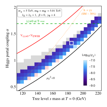
Figure 3: The value of $y_{\chi}=y_{\chi}^{\prime}$ required to obtain the correct relic density $\Omega h^{2}$ [30] for DM mass $m_{\chi}=5$ TeV and $m_{\Psi}=m_{\Psi^{\prime}}=5.01$ TeV. For points plotted in grey, the vev flip-flop occurs but DM depletion is halted by freeze-out of $\Psi_{3}$ and $\Psi_{3}^{\prime}$ rather than the electroweak phase transition. At points shown in pink the equilibrium abundance of $\chi$ is still too high at $T_{n}$, and as inverse decays ensure that the DM density can never drop below its equilibrium value, this implies DM overproduction. Outside the pixelated region, the vev flip-flop does not occur. The red and black lines give tree level estimates for the boundaries of this region. Above the dotted orange line, the decay rate for $h\to\gamma\gamma$ is lower than the SM prediction by more than 30%. Above the dashed green line the $\mathbb{Z}_{3}$ symmetry is broken in the high $T$ limit.

Parameter Space.—We now depart from the particular parameter point considered in figs. 1 and 2 and consider a wider range of parameter space in fig. 3, which shows the $m_{s}$–$\alpha$ plane. Here, $m_{s}$ refers to the tree level $s$ mass at $T=0$. Note that for $\alpha\gtrsim 5$ the perturbative expansion may no longer be reliable [14, 31], but for the $\alpha$ values shown in fig. 3 there is no problem.

We highlight the region where the observed relic density can be obtained from the vev flip-flop, with the blue colour-code indicating the requisite value of $y_{\chi}=y_{\chi}^{\prime}$. We see that this is usually possible provided the vev flip-flop occurs at all (pixelated area in fig. 3). At parameter points shown in grey, the $\Psi_{3}$, $\Psi_{3}^{\prime}$ annihilation rate at the nucleation temperature $\sim(y_{\Psi}^{4}/m_{\Psi}^{2})[m_{\Psi}T_{n}/(2\pi)]^{3/2}\exp(-m_{\Psi}/T_{n})$ is lower than the Hubble rate $\sim T_{n}^{2}/M_{\text{Pl}}$, implying that the depletion of dark sector particles is halted by $\Psi_{3}$, $\Psi_{3}^{\prime}$ rather than the electroweak phase transition. This can change if the DM mass is lower, $y_{\Psi}$ is larger, or extra annihilation modes for $\Psi_{3}$ and $\Psi_{3}^{\prime}$ are introduced. Points with too high $T_{n}$ (shown in pink), could be rescued by increasing $m_{\chi}$.

Below the black line in fig. 3, $\mu_{S}^{2}$ is negative at tree level, so the $\mathbb{Z}_{3}$ symmetry is never broken at tree-level. Above the red line, $\mu_{S}^{2}>0$ is so large at tree level that the Universe never leaves the ${\langle s\rangle}\neq 0$, ${\langle h\rangle}=0$ phase. By comparing with the edge of the pixelated region, where the vev flip-flop occurs, we see that these tree level estimates are only rough approximations to the full one-loop $T$ dependent behaviour. Above the dashed green line, our model is in the phase with broken $\mathbb{Z}_{3}$ and $SU(2)_{L}$ symmetries in the $T\to\infty$ limit. In this regime, the positive daisy corrections to $\mu_{S}^{2}$ are larger than the negative one-loop corrections in the high-$T$ limit. In principle, $\chi$ decays are then sensitive to higher scale physics, but since most decays still happen just above the electroweak phase transition, our calculations, which begin at $T=1$ TeV, remain valid.

Constraints and Future Tests.—The flip-flopping vevs model presented here is mainly constrained by collider searches as direct and indirect detection of $\chi$ are hindered by the smallness of $y_{\chi}$, $y_{\chi}^{\prime}$. For direct and indirect searches, the subdominant population of $S_{3}$, $\Psi_{3}$, $\Psi_{3}^{\prime}$ offers the best detection prospects.

At the LHC or a possible future collider, the most promising direct discovery channel is Drell–Yan production of $s^{\pm}$ pairs through their electromagnetic interactions, followed by the decay $s^{\pm}\to s+W^{*\pm}$. Due to the small mass splitting between the charged and neutral components of the triplets, these decays will typically be too soft to be observed directly, so that the sensitivity to the model will come mainly from mono-$X$ searches. At present, these searches still fall several orders of magnitude short of probing the interesting region of parameter space [29]. For very small mass splittings $<m_{\pi}\sim 140$ MeV, charged track searches could be sensitive [37, 38, 39], but reducing the mass splitting this far would require tuning between a small non-zero value of the coupling constant $\beta$ and electroweak radiative corrections. Perhaps the most promising probe of our vev flip-flop model at the LHC is the precision measurement of the $h\to\gamma\gamma$ rate. Indeed, as shown in fig. 3, sizeable deviations from the SM rate for this decay are predicted. In fact, the present limit would already appear to be in some tension with our model at the $2\sigma$ level [40, 41] due to an event excess in the 7+8 TeV data from ATLAS and CMS. This statement is, however, put into perspective when taking into account that at $\sqrt{s}=13$ TeV, both experiments have observed an event deficit [42, 43].

Summary.—We have presented a novel mechanism for generating the observed relic abundance of electroweak scale DM utilising a temporary period of dark matter decay at the weak scale. In this scenario, the DM abundance today is governed by the dynamics of the scalar potential. We have demonstrated the mechanism in a simple Higgs portal model, focusing on a region of parameter space where dark matter freezes out while relativistic. The initial overabundance is depleted after the $\mathbb{Z}_{3}$ symmetry that stabilises dark matter is spontaneously broken and DM decays. At a later point the Universe undergoes a first order phase transition that restores the dark sector $\mathbb{Z}_{3}$ symmetry and breaks $SU(2)_{L}\times U(1)_{Y}$. Finally, we have outlined avenues for testing this scenario at colliders.

Acknowledgements.—We would like to thank the members of the DFG Research Unit “New Physics at the LHC”, especially Jan Heisig and Susanne Westhoff, for many useful discussions. We are moreover indebted to Jonathan Kozaczuk for invaluable advice on using CosmoTransitions. JK would like to thank Moshe Moshe for interesting conversations. We also appreciate suggestions made by Tim Cohen, Brian Shuve and Andi Hektor. We would like to thank CERN and Fermilab for kind hospitality and support during crucial stages of this project. This work was in part supported by the German Research Foundation (DFG) under Grant Nos. KO 4820/1–1 and FOR 2239, and by the European Research Council (ERC) under the European Union’s Horizon 2020 research and innovation programme (grant agreement No. 637506, “$\nu$Directions”).

Appendix A Appendix A: The Scalar Potential at Finite $T$.

Here we give the finite temperature corrections to the scalar potential in eq. 1. These corrections are dominated by contributions from the scalars ($H$ and $S_{3}$), the electroweak gauge bosons and the top quark. The other SM fermions couple very weakly to $H$, while the new fermions $\chi$, $\Psi_{3}$ and $\Psi_{3}^{\prime}$ are heavy and decouple at the temperatures under consideration. The field dependent masses of the CP even neutral scalars in the basis $(h,s)$ are given by

$$\begin{pmatrix}-\mu_{H}^{2}+3\lambda h^{2}+\frac{1}{2}\alpha s^{2}&\alpha hs\\ \alpha hs&-\mu_{S}^{2}+3\lambda_{S}s^{2}+\frac{1}{2}\alpha h^{2}\end{pmatrix}.$$ (3)

The charged scalars, in the basis $(s^{+},s^{-},G^{+})$, have the mass matrix

$$\begin{pmatrix}-\mu_{S}^{2}+\frac{1}{4}(2\alpha-\beta)h^{2}+(\lambda_{S}+\lambda_{3})s^{2}&\lambda_{3}s^{2}&\frac{\beta hs}{2\sqrt{2}}\\ \lambda_{3}s^{2}&-\mu_{S}^{2}+\frac{1}{4}(2\alpha+\beta)h^{2}+(\lambda_{S}+\lambda_{3})s^{2}&\frac{\beta hs}{2\sqrt{2}}\\ \frac{\beta hs}{2\sqrt{2}}&\frac{\beta hs}{2\sqrt{2}}&-\mu_{H}^{2}+\lambda_{H}h^{2}+\frac{\alpha s^{2}}{2}\end{pmatrix}.$$ (4)

The field dependent masses of the remaining fields are

$$m_{a}^{2} =-\mu_{S}^{2}+\frac{1}{2}\alpha h^{2}+\lambda_{S}s^{2}\,,$$ (5)

$$m_{G^{0}}^{2} =-\mu_{H}^{2}+\frac{1}{2}\alpha s^{2}+\lambda_{H}h^{2}\,,$$ (6)

$$m_{W^{\pm}}^{2} =\frac{1}{4}g^{2}(h^{2}+4s^{2})\,,$$ (7)

$$m_{Z}^{2} =\frac{1}{4}(g^{2}+g^{\prime 2})h^{2}\,,$$ (8)

$$m_{\gamma}^{2} =0\,,$$ (9)

$$m_{t}^{2} =\frac{1}{2}y_{t}^{2}h^{2}\,.$$ (10)

Here, $y_{t}$ is the top quark Yukawa coupling and $g$ and $g^{\prime}$ are the SM $SU(2)_{L}$ and $U(1)_{Y}$ coupling constants, respectively.

The $T$-independent Coleman-Weinberg contribution is [16, 19]

$$V^{\text{CW}}(h,s) =\sum_{i}\frac{n_{i}}{64\pi^{2}}m_{i}^{4}(h,s)\left[\log\frac{m_{i}^{2}(h,s)}{\Lambda^{2}}-C_{i}\right],$$ (11)

where the sum is over the eigenvalues of the mass matrices of $\{h,G^{0},G^{+},s,a,s^{+},s^{-},W,Z,t\}$ and $n_{h}=n_{s}=n_{a}=n_{G^{0}}=1$, $n_{G^{+}}=n_{s^{\pm}}=2$, $n_{Z}=3$, $n_{W}=6$ and $n_{t}=-12$ accounts for their degrees of freedom. We take the renormalisation scale $\Lambda$ to be the SM Higgs vev $v=246$ GeV. In the dimensional regularisation scheme $C_{i}=5/6\,(3/2)$ for gauge bosons (scalars and fermions). We also add counterterms to ensure that $v=\mu_{H}/\sqrt{\lambda_{H}}$ and $m_{h}=\sqrt{2}\mu_{H}$ at $T=0$.

The one-loop finite temperature correction is [17]

$$V^{T}(h,s)= \sum_{i}\frac{n_{i}T^{4}}{2\pi^{2}}\int_{0}^{\infty}\!dx\,x^{2}$$

$$\times\log\bigg{[}1\pm\exp\Big{(}-\sqrt{x^{2}+m_{i}^{2}(h,s)/T^{2}}\Big{)}\bigg{]}\,,$$ (12)

where we sum over the same eigenvalues as for the Coleman-Weinberg contribution. The negative sign in the integrand is for bosons while the positive sign is for fermions.

The bosons also contribute to higher order “daisy” diagrams which can be resummed to give [18]

$$V^{\text{daisy}} =-\frac{T}{12\pi}\sum_{i}n_{i}\Big{(}\left[m^{2}(h,s)+\Pi(T)\right]_{i}^{\frac{3}{2}}$$

$$\hskip 85.35826pt-\left[m_{i}^{2}(h,s)\right]_{i}^{\frac{3}{2}}\Big{)}\,.$$ (13)

Here, the first term should be interpreted as the $i$-th eigenvalue of the matrix-valued quantity $[m^{2}(h,s)+\Pi(T)]^{3/2}$, where $m^{2}(h,s)$ is the block-diagonal matrix composed of the individual mass matrices in eqs. 3 to 9 [27]. The sum runs over the bosonic degrees of freedom: $i\in\{h,G^{0},G^{+},s,a,s^{+},s^{-},W^{i},B\}$. The bosonic thermal masses (Debye masses) in the gauge basis are given by

$$\Pi_{h,G^{0},G^{+}} =\frac{T^{2}}{16}\left(3g^{2}+g^{\prime 2}+4\alpha+8\lambda_{H}+4y_{t}^{2}\right)\,,$$ (14)

$$\Pi_{s,a,s^{+},s^{-}} =\frac{T^{2}}{6}\left(3g^{2}+\alpha+2\lambda_{3}+4\lambda_{S}\right)\,,$$ (15)

$$\Pi_{W^{1,2,3}}^{L} =\frac{5}{2}g^{2}T^{2}\,\qquad\Pi_{W^{1,2,3}}^{T}=0\,,$$ (16)

$$\Pi_{B}^{L} =\frac{11}{6}g^{\prime 2}T^{2}\,,\qquad\Pi_{B}^{T}=0.$$ (17)

Since only the longitudinal components of the gauge bosons contribute, $n_{W^{i}}^{L}=n_{B}^{L}=1$.

Appendix B Appendix B: Dark Matter Decay Rates.

When $\left\langle s\right\rangle\neq 0$, the fermion $\chi$ can mix into $\Psi_{3}$ and $\Psi_{3}^{\prime}$ and decay via a $W$ boson. When kinematically allowed, $\chi$ can also decay into components of $\Psi_{3}$ or $\Psi_{3}^{\prime}$ and a component of $S_{3}$. We will denote the mass eigenstates of the charged fermions as $\widetilde{\Psi}^{+}_{1,2}$, and we will make use of the functions

$$\Gamma_{V}(W,\psi) =\frac{\sqrt{[m_{\chi}^{2}-(m_{W}-m_{\psi})^{2}][m_{\chi}^{2}-(m_{W}+m_{\psi})^{2}]}}{16\pi m_{W}^{2}m_{\chi}^{3}}\Big{[}-2m_{W}^{4}+m_{W}^{2}(m_{\chi}^{2}-6m_{\chi}m_{\psi}+m_{\psi}^{2})+(m_{\chi}^{2}-m_{\psi}^{2})^{2}\Big{]}\,,$$ (18)

$$\Gamma_{S}(s,\psi) =\frac{\sqrt{[m_{\chi}^{2}-(m_{s}-m_{\psi})^{2}][m_{\chi}^{2}-(m_{s}+m_{\psi})^{2}]}}{16\pi m_{\chi}^{3}}\Big{[}(m_{\chi}+m_{\psi})^{2}-m_{s}^{2}\Big{]}\,.$$ (19)

Taking $y_{\chi}=y_{\chi}^{\prime}$, we find the total decay rate to be

$$\Gamma_{\chi} =g^{2}\sin^{2}\theta\big{[}\Gamma_{V}(W,\widetilde{\psi}^{+}_{1})+\Gamma_{V}(W,\widetilde{\psi}^{+}_{2})\big{]}+y_{\chi}^{2}\Gamma_{S}(s,\psi^{0})$$

$$+\left(y_{\chi}^{2}+\frac{y_{\Psi}^{2}\sin^{2}\theta}{2}\right)\big{[}\Gamma_{S}(s^{+},\widetilde{\Psi}^{+}_{1})+\Gamma_{S}(s^{+},\widetilde{\Psi}^{+}_{2})\big{]}\,.$$ (20)

The mixing angle is $\theta\simeq y_{\chi}\left\langle s\right\rangle/(m_{\Psi}-m_{\chi})$, where we have used the small angle approximation. This is justified since $y_{\chi}\lesssim 10^{-7}$ and $\left\langle s\right\rangle\sim(m_{\Psi}-m_{\chi})$. Since the mixing angle is small, we neglect the resulting change in the $\chi$ and $\Psi^{0}$ mass eigenvalues.

Appendix C Appendix C: Computation of the Dark Matter Abundance.

To compute the DM abundance today in the vev flip-flop scenario, we need to solve the coupled Boltzmann equations

$$\dot{n}_{\chi}^{j}+3Hn_{\chi}^{j}=-\frac{\Gamma}{\gamma^{j}}\big{(}n_{\chi}^{j}-n_{\chi}^{j,\text{eq}}\big{)}$$ (21)

together with the Friedmann equation

$$H^{2}=\bigg{(}\frac{\dot{a}}{a}\bigg{)}^{2}=\frac{8\pi G_{N}}{3}\big{(}\rho_{\text{SM}}+\rho_{\chi}\big{)}\,.$$ (22)

In these equations, $n_{\chi}^{j}$ denotes the number density of DM particles in a comoving momentum interval centred at a momentum $p^{j}$, and $n_{\chi}^{j,\text{eq}}$ is the corresponding equilibrium abundance. We use 128 such intervals, covering the momentum range from 0 to 1000 TeV at $T=10$ TeV. We have checked that increasing the momentum range or resolution does not alter our results. The DM energy density is obtained from $n_{\chi}^{j}$ according to $\rho_{\chi}\equiv\sum_{j}E^{j}n_{\chi}^{j}$, where $E^{j}=[(p^{j})^{2}+m_{\chi}^{2}]^{1/2}$, and the energy density of SM particles is given by $\rho_{\text{SM}}=g_{*}(\pi^{2}/30)T^{4}$, with $g_{*}$ the effective number of SM degrees of freedom. The decay rate $\Gamma$ depends on temperature through $m_{s}$, $m_{h}$ and ${\langle s\rangle}$, but is independent of momentum. The relativistic gamma factor is given by $\gamma^{j}=E_{j}/m_{\chi}$.

To solve eqs. 21 and 22 in practice, we make the substitution $Y^{j}\equiv n^{j}/s$, where $s=g_{*}(2\pi^{2}/45)T^{3}$ is the entropy density in SM degrees of freedom. We moreover need a relation between time $t$ and temperature $T$. To find it, note that

$$\dot{\rho}_{\text{SM}}=4\rho_{\text{SM}}\frac{\dot{T}}{T}=m_{\chi}\sum_{j}\frac{\Gamma}{\gamma^{j}}\big{(}n_{\chi}^{j}-n_{\chi}^{j,\text{eq}}\big{)}-4H\rho_{\text{SM}}\,.$$ (23)

The first term on the right hand side corresponds to energy injection into the SM plasma from DM decays, the second one corresponds to energy dissipation by redshifting. It follows that

$$\frac{dT}{dt}=\sum_{j}\big{(}n_{\chi}^{j}-n_{\chi}^{j,\text{eq}}\big{)}\frac{m_{\chi}\Gamma T}{4\gamma^{j}\rho_{\text{SM}}}-HT\,.$$ (24)

References

- [1] LUX Collaboration, A. Manalaysay, Dark-matter results from 332 new live days of LUX data, . Identification of Dark Matter 2016 slides.
- [2] PandaX-II Collaboration, A. Tan et al., Dark Matter Results from First 98.7-day Data of PandaX-II Experiment, arXiv:1607.07400.
- [3] Fermi-LAT Collaboration, M. Ackermann et al., Searching for Dark Matter Annihilation from Milky Way Dwarf Spheroidal Galaxies with Six Years of Fermi Large Area Telescope Data, Phys. Rev. Lett. 115 (2015), no. 23 231301, [arXiv:1503.02641].
- [4] AMS-02 Collaboration, C. Pizzolotto, Positron fraction, electron and positron spectra measured by AMS-02, EPJ Web Conf. 121 (2016) 03006.
- [5] M. S. Madhavacheril, N. Sehgal, and T. R. Slatyer, Current Dark Matter Annihilation Constraints from CMB and Low-Redshift Data, Phys. Rev. D89 (2014) 103508, [arXiv:1310.3815].
- [6] ATLAS Collaboration, M. Aaboud et al., Search for new phenomena in final states with an energetic jet and large missing transverse momentum in collisions at TeV using the ATLAS detector, arXiv:1604.07773.
- [7] CMS Collaboration, Search for dark matter in final states with an energetic jet, or a hadronically decaying W or Z boson using of data at , . CMS-PAS-EXO-16-037.
- [8] S. Profumo, M. J. Ramsey-Musolf, and G. Shaughnessy, Singlet Higgs phenomenology and the electroweak phase transition, JHEP 08 (2007) 010, [arXiv:0705.2425].
- [9] J. M. Cline, G. Laporte, H. Yamashita, and S. Kraml, Electroweak Phase Transition and LHC Signatures in the Singlet Majoron Model, JHEP 07 (2009) 040, [arXiv:0905.2559].
- [10] J. R. Espinosa, T. Konstandin, and F. Riva, Strong Electroweak Phase Transitions in the Standard Model with a Singlet, Nucl. Phys. B854 (2012) 592–630, [arXiv:1107.5441].
- [11] Y. Cui, L. Randall, and B. Shuve, Emergent Dark Matter, Baryon, and Lepton Numbers, JHEP 08 (2011) 073, [arXiv:1106.4834].
- [12] J. M. Cline and K. Kainulainen, Electroweak baryogenesis and dark matter from a singlet Higgs, JCAP 1301 (2013) 012, [arXiv:1210.4196].
- [13] M. Fairbairn and R. Hogan, Singlet Fermionic Dark Matter and the Electroweak Phase Transition, JHEP 09 (2013) 022, [arXiv:1305.3452].
- [14] D. Curtin, P. Meade, and C.-T. Yu, Testing Electroweak Baryogenesis with Future Colliders, JHEP 11 (2014) 127, [arXiv:1409.0005].
- [15] T. Cohen, D. E. Morrissey, and A. Pierce, Changes in Dark Matter Properties After Freeze-Out, Phys. Rev. D78 (2008) 111701, [arXiv:0808.3994].
- [16] S. R. Coleman and E. J. Weinberg, Radiative Corrections as the Origin of Spontaneous Symmetry Breaking, Phys. Rev. D7 (1973) 1888–1910.
- [17] L. Dolan and R. Jackiw, Symmetry Behavior at Finite Temperature, Phys. Rev. D9 (1974) 3320–3341.
- [18] M. E. Carrington, The Effective potential at finite temperature in the Standard Model, Phys. Rev. D45 (1992) 2933–2944.
- [19] M. Quiros, Finite temperature field theory and phase transitions, in Proceedings, Summer School in High-energy physics and cosmology: Trieste, Italy, June 29-July 17, 1998, pp. 187–259, 1999. hep-ph/9901312.
- [20] A. Ahriche, What is the criterion for a strong first order electroweak phase transition in singlet models?, Phys. Rev. D75 (2007) 083522, [hep-ph/0701192].
- [21] C. Delaunay, C. Grojean, and J. D. Wells, Dynamics of Non-renormalizable Electroweak Symmetry Breaking, JHEP 04 (2008) 029, [arXiv:0711.2511].
- [22] A. D. Linde, Decay of the False Vacuum at Finite Temperature, Nucl. Phys. B216 (1983) 421. [Erratum: Nucl. Phys.B223,544(1983)].
- [23] C. L. Wainwright, CosmoTransitions: Computing Cosmological Phase Transition Temperatures and Bubble Profiles with Multiple Fields, Comput. Phys. Commun. 183 (2012) 2006–2013, [arXiv:1109.4189].
- [24] J. Kozaczuk, S. Profumo, L. S. Haskins, and C. L. Wainwright, Cosmological Phase Transitions and their Properties in the NMSSM, JHEP 01 (2015) 144, [arXiv:1407.4134].
- [25] N. Blinov, J. Kozaczuk, D. E. Morrissey, and C. Tamarit, Electroweak Baryogenesis from Exotic Electroweak Symmetry Breaking, Phys. Rev. D92 (2015), no. 3 035012, [arXiv:1504.05195].
- [26] J. Kozaczuk, Bubble Expansion and the Viability of Singlet-Driven Electroweak Baryogenesis, JHEP 10 (2015) 135, [arXiv:1506.04741].
- [27] H. H. Patel and M. J. Ramsey-Musolf, Baryon Washout, Electroweak Phase Transition, and Perturbation Theory, JHEP 07 (2011) 029, [arXiv:1101.4665].
- [28] M. Cirelli and A. Strumia, Minimal Dark Matter: Model and results, New J.Phys. 11 (2009) 105005, [arXiv:0903.3381].
- [29] J. Kopp, E. T. Neil, R. Primulando, and J. Zupan, From gamma ray line signals of dark matter to the LHC, Phys.Dark Univ. 2 (2013) 22–34, [arXiv:1301.1683].
- [30] Planck Collaboration, P. A. R. Ade et al., Planck 2015 results. XIII. Cosmological parameters, Astron. Astrophys. 594 (2016) A13, [arXiv:1502.01589].
- [31] C. Tamarit, Higgs vacua with potential barriers, Phys. Rev. D90 (2014), no. 5 055024, [arXiv:1404.7673].
- [32] V. A. Kuzmin, V. A. Rubakov, and M. E. Shaposhnikov, On the Anomalous Electroweak Baryon Number Nonconservation in the Early Universe, Phys. Lett. B155 (1985) 36.
- [33] M. E. Shaposhnikov, Possible Appearance of the Baryon Asymmetry of the Universe in an Electroweak Theory, JETP Lett. 44 (1986) 465–468. [Pisma Zh. Eksp. Teor. Fiz.44,364(1986)].
- [34] M. E. Shaposhnikov, Baryon Asymmetry of the Universe in Standard Electroweak Theory, Nucl. Phys. B287 (1987) 757–775.
- [35] D. E. Morrissey and M. J. Ramsey-Musolf, Electroweak baryogenesis, New J. Phys. 14 (2012) 125003, [arXiv:1206.2942].
- [36] M. Carena, M. Quiros, and C. E. M. Wagner, Opening the window for electroweak baryogenesis, Phys. Lett. B380 (1996) 81–91, [hep-ph/9603420].
- [37] ATLAS Collaboration, G. Aad et al., Search for long-lived, weakly interacting particles that decay to displaced hadronic jets in proton-proton collisions at TeV with the ATLAS detector, Phys. Rev. D92 (2015), no. 1 012010, [arXiv:1504.03634].
- [38] CMS Collaboration, Search for heavy stable charged particles with of 2016 data, . CMS-PAS-EXO-16-036.
- [39] CMS Collaboration, Search for displaced leptons in the e-mu channel, . CMS-PAS-EXO-16-022.
- [40] ATLAS, CMS Collaboration, G. Aad et al., Measurements of the Higgs boson production and decay rates and constraints on its couplings from a combined ATLAS and CMS analysis of the LHC pp collision data at and 8 TeV, JHEP 08 (2016) 045, [arXiv:1606.02266].
- [41] Particle Data Group Collaboration, C. Patrignani et al., Review of Particle Physics, Chin. Phys. C40 (2016), no. 10 100001.
- [42] CMS Collaboration Collaboration, Updated measurements of Higgs boson production in the diphoton decay channel at in pp collisions at CMS., Tech. Rep. CMS-PAS-HIG-16-020, CERN, Geneva, 2016.
- [43] ATLAS Collaboration Collaboration, Measurement of fiducial, differential and production cross sections in the decay channel with 13.3 fb-1 of 13 TeV proton-proton collision data with the ATLAS detector, Tech. Rep. ATLAS-CONF-2016-067, CERN, Geneva, Aug, 2016.