Activity Networks with Delays
An application to toxicity analysis

Abstract

ANDy, Activity Networks with Delays, is a discrete time framework aimed at the qualitative modelling of time-dependent activities. The modular and concise syntax makes ANDy suitable for an easy and natural modelling of time-dependent biological systems (i.e., regulatory pathways).

Activities involve entities playing the role of activators, inhibitors or products of biochemical network operation. Activities may have given duration, i.e., the time required to obtain results. An entity may represent an object (e.g., an agent, a biochemical species or a family of thereof) with a local attribute, a state denoting its level (e.g., concentration, strength). Entities levels may change as a result of an activity or may decay gradually as time passes by.

The semantics of ANDy is formally given via high-level Petri nets ensuring this way some modularity. As main results we show that ANDy systems have finite state representations even for potentially infinite processes and it well adapts to the modelling of toxic behaviours. As an illustration, we present a classification of toxicity properties and give some hints on how they can be verified with existing tools on ANDy systems. A small case study on blood glucose regulation is provided to exemplify the ANDy framework and the toxicity properties.

1 Introduction

Activities and their causal relationships are a central concern in biological systems such as biological networks and regulatory pathways. They deal with questions such as, how long does it take to complete an activity, when it can be performed, or whether it can be delayed or even ignored. Our proposal stems from reaction systems [1], a formalism based on reactions, each defined as a triple $(R,I,P)$ with $R$ set of reactants, $I$ set of inhibitors and $P$ set of products, and $R,I$ and $P$ taken from a common set of species. Reaction systems are based on three basic assumptions:

1. a reaction can take place only if all the reactants involved are available but none of the inhibitors are;

2. if a species is available then a sufficient amount of it is necessary to trigger a reaction;

3. species are not persistent: they become unavailable if they are not sustained by a reaction.

We complement this model by adding several important features. We allow a richer description of species states using attributes having potentially multiple values and introduce timing aspects. More precisely, the resulting formalism, Activity Networks with Delays (ANDy), targets systems composed of various entities (i.e., species in reaction systems) that evolve by means of time-dependent activities. Each entity is characterised by one attribute, called level, representing rates, activation/inhibition status or expression degrees (e.g., low, medium, high). Activities are rules describing the evolution of systems, involving (as for reaction systems) three sets of entities: activators, which must be present, inhibitors, which must be absent, and results whose expression levels have to be modified (increased or decreased). The introduction of time concerns both activities and entities. Activities have a duration and entities are subject to a decay process or aging that models the action of a non-specified environment: i.e., levels decrease with time progression. Another difference is in the semantics of activities: while in reaction systems a maximal concurrency model is considered, here we adopt two types of activities: mandatory and potential ones. The former set of activities, once enabled, must take place altogether in the same time unit (in maximal concurrency) while the latter, non deterministically one at the time, may be performed or not. Following [2], as in our modelling all entities have discrete states and share the same global clock, it is reasonable to work with discrete time constraints.

Our main objective is to provide theoretical foundations and underlying tools for the description and the understanding of the mechanisms and of the structural properties underpinning biological interactions networks. In biology, ordinary differential equations (ODE) remain the predominant modelling methodology[3]. Such models present however some drawbacks: they need a precise quantification of parameters, random interactions are difficult to model outside an averaged approach, system openness and non-linearities make hopeless the existence of analytic solutions, and numerical methods – often the only sensible option – are mainly descriptive and cannot form the basis for an explanatory theory. On the other hand, many languages and tools have been developed to build and explore discrete qualitative models in various application domains. Such models are rough abstractions of real world processes but they make possible to unravel the entangled causal relationships between system’s entities. More specifically in systems biology, formalisms like Petri nets [4], Boolean networks [5], process algebras [6] or rewriting systems [7] (to cite a few) have been used with undeniable success to understand the causal links between structure and behaviour in molecular networks. Nonetheless, the management of time is somewhat problematic in all of the previous approaches. In general, timing aspects are either disregarded or handled at a primitive level, which leads to expressiveness problems for the modeller. For example, modelling a synchronous evolution directly in Petri nets requires a coding that is not necessarily natural for a biologist. This is why here we propose a qualitative discrete formalism for biological systems that provides, in particular, a direct and intuitive account of timing aspects natural in biology such as activity duration and decay. Such features are in particular essential in describing toxicity problems. Indeed toxicology [8] studies the adverse effects of the exposures to chemicals at various levels of living entities: organism, tissue, cell and intracellular molecular systems. During the last decade, the accumulation of genomic and post-genomic data together with the introduction of new technologies for gene analysis has opened the way to toxicogenomics. Toxicogenomics combines toxicology with “Omics” technologies to study the mode-of-action of toxicants or environmental stressors on biological systems. The mode-of-action is understood as the sequence of events from the absorption of chemicals to a toxic outcome. Toxicogenomics potentially improves clinical diagnosis capabilities and facilitates the identification of potential toxicity in drug discovery [9] or in the design of bio-synthetic entities [10]. Our formalism permits to model biological systems together with their stressors and discover (or highlight) the mode-of-action of toxicants, that is why we complement our designing process with a general discussion on toxicity properties and how they can be tested against ANDy systems. In this respect, we aim at providing a methodology rather than a precise technique of testing.

Organisation of the paper.

This paper is the extended version of BioPPN workshop paper [11]. The main difference with respect to [11] is the introduction of time aspects in ANDy systems, a more mature taxonomy of toxicity properties and a prototype implementation of ANDy networks using Snakes toolkit [12], Snoopy [13] and its related analysis tool Charlie [14].

Section 2 introduces the principles behind ANDy networks and gives a formal definition of ANDy semantics in terms of high-level Petri nets. It also states the main result of the paper addressing the finiteness of state space. Next, Section 3 discusses an axiomatisation of toxicity properties. An illustration of the model and its properties is given in Section 4 describing the assimilation of aspartame in blood regulation in human body. Finally Sections 5 and 6 discuss related works and conclude.

A web page with additional material is available at [15]. It includes the implementations in Snakes and Snoopy and a technical report adding a comparison with timed automata.

2 Activity Networks with Delays

In this section we give the syntax and semantics of Activity Networks with Delays (ANDy). An ANDy is composed by a set of entities $\mathcal{E}$ driven by a set of timed activities. The time is assumed to be discrete and modelled by a tick event.

Entities.

Each entity, $e\in\mathcal{E}$, is associated to a finite number of levels $\mathcal{L}_{e}$ (from 0 to $\mathcal{L}_{e}-1$) that in general represent ordered expression degrees (e.g., low, medium, high) and refer to a change in the entity capability of action. A decay duration is associated to each level of an entity $e$ through the function $\delta_{e}:[0\,.\,.\,\mathcal{L}_{e}-1]\to{\rm Nature}^{+}\cup\{\omega\}$ allowing different duration’s for different levels or $\omega$ if unbounded. More precisely, if $\delta_{e}(i)=\omega$, then level $i$ is permanent and it can be modified only by an activity. If $\delta_{e}(i)\neq\omega$, the presence of the entity at level $i$ is transient: once entity $e$ at level $i$ has passed $\delta_{e}(i)$ time units its level will pass to $i-1$, i.e., it decays or ages gradually as time passes by. We fix $\delta_{e}(0)=\omega$ as no negative level is allowed. In principle, this substitutes a set of unspecified activities accounting for the action of an underspecified environment that consumes entities. A state $\mathsf{s}$ of an ANDy network assigns to each entity $e\in\mathcal{E}$ a level $\eta\in[0..\mathcal{L}_{e}-1]$. The initial state $\mathsf{s}_{0}$ sets each entity $e$ to a given level $\eta_{e}$.

Activities.

The evolution of entities is driven by timed activities of the form:

$$\rho::=A_{\rho};I_{\rho}\xrightarrow{\Delta_{\rho}}R_{\rho}$$

where $\Delta_{\rho}\in{\rm Nature}$ is the activity duration, $A_{\rho}$ (activators) and $I_{\rho}$ (inhibitors) are sets of pairs $(e,\eta_{e})$ with $e\in\mathcal{E}$ and $\eta_{e}\in[0\,.\,.\,\mathcal{L}_{e}-1]$; $R_{\rho}$, the results, is a non empty set of pairs $(e,\pm n)$ where $e\in\mathcal{E}$ and $\pm n\in\mathbb{Z}$ is a positive or negative variation of the entity level $\eta_{e}$. Entities can appear at most once in each set $A_{\rho}$, $I_{\rho}$ and $R_{\rho}$, cf., Remark 2.2 below. We write $e\in A_{\rho}$ to denote $(e,\cdot)\in A_{\rho}$, similarly for $I_{\rho}$ and $R_{\rho}$. We omit index $\rho$ if it is clear from the context.

Duration $\Delta_{\rho}$ characterises the number of ticks required for yielding change of levels of results, $\Delta_{\rho}=0$ denotes an instantaneous activity. The results of an activity are the increments or decrements $\pm n$ of each entity level in $R_{\rho}$ (up to the range of entity levels). An activity $\rho$ can take place only if it is enabled, this depends on the activator and inhibitor levels appearing in $A_{\rho}$ and $I_{\rho}$. Nonetheless, observing only the current level of each entity is not enough to decide if an activity is enabled: such approach would miss the handling of decays and durations.

Definition 2.1 (Enabled activity)

An activity $\rho$ is enabled (i.e., may happen) if and only if:

• for each entity $e_{a}$ of the activators set $A_{\rho}$ (i.e., $(e_{a},\eta_{a})\in A_{\rho}$), $e_{a}$ is available at least at level $\eta_{a}$ for the whole duration $\Delta_{\rho}$;

• for each entity $e_{i}$ of the inhibitors set $I_{\rho}$ (i.e., $(e_{i},\eta_{i})\in I_{\rho}$), $e_{i}$ is available at a level strictly inferior to $\eta_{i}$ for the whole duration $\Delta_{\rho}$;

Remark 2.2

Notice that:

• If an entity is an activator (resp. an inhibitor) at level $\ell$ for some activity $\rho$, it is also an activator (resp. an inhibitor) for $\rho$ at all levels $l\geq\ell$ (resp. $l\leq\ell$).

• An entity may be both in $A$ and $R$, e.g., as in an auto-catalytic production where reaction products themselves are activators for the reaction. Similarly, an entity may be both in $I$ and $R$: thus representing self-repressing activities.

• An entity can appear in the same activity simultaneously as an activator and as an inhibitor but we require them to occur with different levels. For instance, the rule

  $$\{({e},\eta)\}\cup A;\{({e},\eta^{\prime})\}\cup I\xrightarrow{\Delta}R\qquad\text{where\leavevmode\nobreak\ }\eta<\eta^{\prime}$$

  requires that the activity takes place only if the level $l_{e}$ of ${e}$ belongs to the interval $\eta\leq l_{e}<\eta^{\prime}$. In particular, if ${e}$ has to be present in an activity exactly at level $\eta$, ${e}$ should appear as an activator at level $\eta$ and as inhibitor at level $\eta^{\prime}=\eta+1$.

• The set of activators and inhibitors $A\cup I$ is allowed to be empty. In this case, the activity is constantly enabled. This accounts for modelling an environment that continuously sustains the production of an entity. In this case a duration $\Delta\not=0$ may be used to account for a start-up time.

Guided by the case study and the biological applications, we assume that once an activity $\rho$ is triggered:

• it must wait at least $\Delta_{\rho}$ before being enabled again (a kind of refractory period).

• its activators and inhibitors are left unchanged.

These are non restrictive hypotheses and by slightly modifying Definition 2.6 one can obtain different semantics that could depend on the specific modelled scenario: e.g., once enabled an activity $\rho$ can be triggered an unbounded number of times or once per time unit; also one can easily choose a different policy to modify the level of activators and/or inhibitors.

It is important to note that when an activity is enabled, it is not necessarily performed. The idea is to make a distinction between two types of activities:

1. potential activities, denoted by $\alpha$ in a set $\mathcal{P}$: if enabled, they may occur in an interleaved way thus the result depends on the order they are performed. It may happen that no potential activities occur even if they are enabled;

2. mandatory activities, denoted by $\beta$ in a set $\mathcal{M}$: if enabled they must occur within the same time unit. All enabled mandatory activities occur simultaneously.

As all mandatory activities $\beta_{i}$ are triggered simultaneously, all updates related to an entity $e$ are collected and summed up before being applied to the current level of $e$.

Definition 2.3 (ANDy network and its semantics)

An ANDy network is a triple $(\mathcal{E},\mathcal{M},\mathcal{P})$ where $\mathcal{E}$ is the set of entities, $\mathcal{M}$ is the set of mandatory activities and $\mathcal{P}$ is the set of potential ones. It evolves by triggering enabled activities in two separate phases implementing one evolution step:

1. In this phase (between two ticks) potential activities that are enabled may be triggered. Their action occurs non-deterministically in an interleaved way. Any potential activity is triggered at most once in this phase.

2. This phase is the tick transition: the effect is that all concerned entities must decay and all enabled mandatory activities are performed simultaneously. Notice that as activators and inhibitors are not “consumed”, there are no conflicts and so there is a unique way (per time unit) to execute all enabled mandatory activities.

Example 2.4 (Repressilator)

The repressilator [16] is a synthetic genetic regulatory network in Escherichia Coli consisting of three genes ($lacI,tetR,cI$) connected in a feedback loop such that each gene inhibits the next gene and is inhibited by the previous one. The repressilator exhibits a stable oscillation with fixed time period that is witnessed by the synthesis of a green fluorescent protein ($GFP$). According to [16]: “the resulting oscillation with typical periods of hours are slower than the cell division cycle so the state of the oscillator has to be transmitted from generation to generation”.

It may be modelled in ANDy with five entities $\mathcal{E}=\{lacI,tetR,cI,GFP,gen\}$. The first three represent the three genes, each with two levels denoting an on/off state where level $1=on$ has decay time $2$. $GFP$ has two levels (on/off) with unbounded decay. Finally, the evolution of successive generations is represented by entity $gen$ with, let’s say, seven levels (from 0 to 6, with unbounded decay) to differentiate among generations.

The behaviour is modelled with potential and mandatory activities: potential activities (on the left below) are used to represent the feedback loop between $lacI,tetR$ and $cI$. Mandatory activities (on the right) handle the synthesis of $GFP$ and show the evolution of generations.

$$\begin{array}[]{ll}\alpha_{1}:\emptyset;(lacI,1)\xrightarrow{2}(tetR,+1)&\beta_{1}:(lacI,1);\emptyset\xrightarrow{0}(GFP,+1)\\ \alpha_{2}:\emptyset;(tetR,1)\xrightarrow{2}(cI,+1)&\beta_{2}:(lacI,0);(lacI,1)\xrightarrow{0}(GFP,-1)\\ \alpha_{3}:\emptyset;(cI,1)\xrightarrow{2}(lacI,+1)&\beta_{3}:(gen,0);(gen,6)\xrightarrow{1}(gen,+1)\\ &\beta_{4}:(gen,6);\emptyset\xrightarrow{1}(gen,-6)\end{array}$$

In particular, the evolution of successive generations is circular modulo 7, this allows us to have a finite number of levels for $gen$). Activities $\beta_{3}$ and $\beta_{4}$ describe such a behaviour. Notice in particular the use of inhibitor $(gen,6)$ in $\beta_{3}$ that allows to apply the activity for all levels of $gen$ from 0 to 5 and to apply $\beta_{4}$ for level 6.

We now exhibit a possible execution scenario for the repressilator, the table below shows for each line the current level of each entity:

$$lacI$$ description

0 0 1 0 0  initial state

0 0 1 0 0  after Ph. 2 (tick)

0 0 1 0 0  after Ph. 1 (no activity)

0 0 1 0 1  after Ph. 2 (tick and activity )

0 1 1 0 1  after Ph. 1 (activity )

0 1 1 0 1  after Ph. 2 (tick)

0 1 1 0 1  after Ph. 1 (no activity)

0 1 0 0 2  after Ph. 2 (tick, decay of and activity )

1 1 0 0 2  after Ph. 1 (activity )

1 1 0 0 2  after Ph. 2 (tick)

1 1 0 0 2  after Ph. 1 (no activity)

1 0 0 1 3  after Ph. 2 (tick, decay of and activities )

$\diamond$

2.1 Petri Net formalisation.

The semantics of ANDy networks is formalised in terms of high-level Petri nets. We recall here the notations together with some elements of their semantics [17].

Definition 2.5

A high-level Petri net is a tuple $(P,T,F,L,M_{0})$ where:

• $P$ is the set of places, $T$ is the set of transitions, with $P\cap T=\emptyset$;

• $F\subseteq(P\times T)\cup(T\times P)$ is the set of arcs;

• $L$ is the labelling of $P\cup T\cup F$ defined as follows:

  • $\forall p\in P$, $L(p)$ is a set of values (the type of $p$);

  • $\forall t\in T$, $L(t)$ is a computable Boolean expression (a guard);

  • and $\forall f\in F$, $L(f)$ is a tuple of variables or values.

• $M_{0}$ is the initial marking putting a multiset of values (tokens) in $L(p)$ in each $p\in P$.

The behaviour of high-level Petri nets is defined as usual: markings (states) are functions from places in $P$ to multisets of possibly structured tokens in $L(p)$. A transition $t\in T$ is enabled at marking $M$, if there exists a valuation $\sigma$ of all variables in the labelling of $t$ such that the guard $L(t)$ evaluates to true ($L_{\sigma}(t)=\mathsf{true}$) and there are enough tokens in all input places $p$ of $t$ to satisfy the corresponding input arcs, i.e., $L_{\sigma}((p,t))\in M(p)$ for each input place $p$ of $t$. The firing of $t$ produces the marking $M^{\prime}$: $\forall p\in P,M^{\prime}(p)=M(p)-L_{\sigma}((p,t))+L_{\sigma}((t,p))$ with $L_{\sigma}(f)=0$ if $f\notin F$, $-$ and $+$ are multiset operators for removal and adding of one element, respectively. We denote it by $M[{t}{:}\sigma{\rangle}M^{\prime}$. Observe that for ANDy we are considering a subclass of high-level Petri nets where for each pair place/transition there is either no connection or a loop (an input and an output arc). So, starting from an initial marking associating one token per place, the number of tokens (but not necessary their value) is maintained at each step of the net evolution.

As usual, in figures, places are represented as rounds, transitions as squares, and arcs as directed arrows. By convention, primed version of variables (e.g., $x^{\prime}$) are used to annotate output arcs of transitions, their evaluation is possibly computed using unprimed variables (e.g., $x$) appearing on input arcs. With an abuse of notation, singleton markings are denoted without brackets, the same is used in arc annotations. Also we refer to valuated variables without effectively mentioning the valuation $\sigma$: e.g., we say that the current value of variable $w$ is $w$ instead of $\sigma(w)$. An example of firing is shown in Figure 1.

(a) Before firing.

(b) After firing.

Figure 1: Example of firing of transition $t$ with $\sigma=\{x=5,y=2,x^{\prime}=7\}$.

We say that a marking $M$ is reachable from the initial marking $M_{0}$ if there exists a firing sequence $(t_{1},\sigma_{1}),\,.\,.\,,(t_{n},\sigma_{n})$ such that $M_{0}[{t_{1}}{:}\sigma_{1}{\rangle}M_{1}\,.\,.\,M_{n-1}[{t_{n}}{:}\sigma_{n}{\rangle}M$. The semantics of an initially marked Petri net is a marking graph (transition system) comprising all the reachable markings.

ANDy’s formalisation.

ANDy syntax and semantics of Definition 2.3 are compact and intelligible, thus easily usable in practice as shown in Example 2.4. However, time and the interplay between entity levels, decay and activity durations require a complex machinery to realize the expected behaviour into high-level Petri nets. Nevertheless, the advantage is that this realization is completely transparent to the final user.

In order to properly describe decay and the semantics of activities we need to record three kinds of information:

1. (decay) since how long an entity is at the current level since the last update,

2. (activators) since how long an entity is available at a level less or equal to the current one (recall that levels are inclusive),

3. (inhibitors) since how long a level greater than the current one has been left.

Notice that duration relative to Items 1 and 2 for the current level can be different: i.e., if an entity is continuously sustained by some activities it remains available in the system at the current level for a period that may be longer than the corresponding decay time. Thus Item 1 reports the duration since the last update (i.e., when the activity concerning the entity has been performed) and Item 2 is the duration since the first appearance of the entity at that level.

For this reason, we model each entity $e\in\mathcal{E}$ by a single Petri net place $p_{e}$ carrying tuples $\langle l_{e},u_{e},\lambda_{e}\rangle$ as tokens where $l_{e}$ is the current level of $e$; $u_{e}$ is a counter storing the duration spent in the current level since the last update (Item 1): $0\leq u_{e}\leq\delta_{e}(l_{e})$; and $\lambda_{e}$ is a tuple of counters with $\mathcal{L}_{e}$ fields (one for each level). Each counter $\lambda_{e}[i]$ contains a duration interpreted as follows:

$$\lambda_{e}[i]=\begin{cases}\begin{minipage}{199.16928pt} since how long $e$ has reached level $i$ (Item 2) \end{minipage}&\text{for }0\leq i\leq l_{e}\\ \\ \begin{minipage}{199.16928pt} since how long $e$ has left level $i$ (Item 3)\\ (or $0$ if $e$ has not yet reached $i$). \end{minipage}&\text{for }l_{e}<i\leq\mathcal{L}_{e}-1\end{cases}$$

Each place is initialised to $\langle\eta_{e},0,0^{\mathcal{L}_{e}}\rangle$ where $\eta_{e}$ is the given initial level of $e$ and $0^{\mathcal{L}_{e}}$ denotes vector $\lambda_{e}$ of counters uniformly initialised with zero.

It is worth observing that once a duration in $\lambda$ has reached the maximum duration for all activities ($D=\max\{\Delta_{\rho}\mid\rho\in\mathcal{M}\cup\mathcal{P}\}$) it is useless to increment it, as for all duration greater than $D$, the guards of all activities involving the entity are satisfied.

Notation 2.5

$\lambda\{\raisebox{2.15277pt}{\small$x$}\!/\mbox{\small$[l\,.\,.\,l+n]$}\}$ is the systematic update to $x$ of values in counters $\lambda[l]\,.\,.\,\lambda[l+n]$. We denote by $\mathsf{inc}_{D}(\lambda)$ the increment by one of all values in $\lambda$: i.e., $\forall k\in[0\,.\,.\,\mathcal{L}_{e}-1]$, $\lambda[k]=\min(\lambda[k]+1,D)$ with $D\in{\rm Nature}$.

Every potential activity $\alpha\in\mathcal{P}$ is modelled with a transition $t_{\alpha}$ and a special place $p_{\alpha}$ that ensures that the same activity is not executed more than once every $\Delta_{\alpha}$ time units, complying to Phase Ph. 1 in Definition 2.3. Figure 2(b) details the scheme of the resulting Petri net and defines the arc annotations. Input and output arcs between the same place and transition with the same label (read arcs) are denoted with a double-pointed arrow with a single label. We comment on the conditions (implementing requirements in Definition 2.1) and results of firing of $t_{\alpha}$ corresponding to a potential activity $\alpha=A;I\xrightarrow{\Delta}R$. We have:

• since each activity must wait at least $\Delta$ before being enabled again, place $p_{\alpha}$ retains whether the activity can be performed $w_{\alpha}\geq\Delta$ and after firing the token is set to $0$, ($w^{\prime}_{\alpha}=0$).

• each activator $a\in A$ has to be present at least at level $\eta_{a}$ for at least $\Delta$ time units, this is expressed by guard $l_{a}\geq\eta_{a}\wedge\lambda[\eta_{a}]\geq\Delta$;

• each inhibitor $i\in I$ has not to exceed level $\eta_{i}$ for at least $\Delta$ time units, this is guaranteed by guard $l_{i}<\eta_{i}\wedge\lambda[\eta_{i}]\geq\Delta$;

• the updates on a place $p_{r}$ of a result entity $r$ at level $l_{r}$ containing token $\langle l_{r},u_{r},\lambda_{r}\rangle$, (i.e., $(r,\pm n)\in R$ with $n\in{\rm Nature}$) are performed as follows:

  Increase $+n$:

  $\langle l_{r}+n,0,\lambda_{r}\{\raisebox{2.15277pt}{\small$0$}\!/\mbox{\small$[l_{r}+1\,.\,.\,l_{r}+n]$}\}\rangle$. $l_{r}$ becomes $l_{r}+n$, $u_{r}$ is reset to 0 restarting the counter for level $l_{r}+n$ and $\lambda_{r}$ is updated to record the change to the new level by resetting the counters $\lambda_{r}[i]$ for all levels $i$ from $l_{r}+1$ to $l_{r}+n$.

  Maintenance $0$:

  $\langle l_{r},0,\lambda_{r}\rangle$: the current level is recharged resetting $u_{r}$ to 0.

  Decrease $-n$:

  $\langle l_{r}-n,0,\lambda_{r}\{\raisebox{2.15277pt}{\small$0$}\!/\mbox{\small$[l_{r}-n+1\,.\,.\,l_{r}]$}\}\rangle$. This case is symmetric to the increase one, except for the treatment of $\lambda_{r}$ that is updated by resetting counters $\lambda_{r}[i]$ for all levels $i$ from $l_{r}-n+1$ to $l_{r}$.

(a) Clock transition.

(b) Transition for $\alpha\in\mathcal{P}$.

Figure 2: Scheme of Petri net modelling of ANDy.

Finally, in order to cope with time aspects present in ANDy, we introduce a tick transition $t_{c}$ (Figure 2(a)) that represents the time progression. Its effect is the one described by Phase Ph. 2 in Definition 2.3: it increments counters of entities, takes care of the decay and simultaneously performs all enabled mandatory activities. More precisely:

Time:

All counters in entities tuples are incremented by one: we pass from $\langle l,u,\lambda\rangle$ to $\langle l,u+1,\mathsf{inc}_{D}(\lambda)\rangle$. Counter $u$ remains unchanged for levels of unbounded duration.

Decay:

An entity may stay at level $l$ for $\delta(l)$ time units (i.e., $u\leq\delta(l)$). Decay happens as soon as the interval $\delta(l)$ is elapsed and is obtained by decreasing the level by one, till reaching level zero. We pass from $\langle l,u,\lambda\rangle$ to $\langle l-1,0,\mathsf{inc}_{D}(\lambda)\{\raisebox{2.15277pt}{\small$0$}\!/\mbox{\small$l$}\}\rangle$.

Mandatory activities:

All enabled mandatory activities $\beta$ are performed simultaneously. The results on involved entities are collected and summed up. The derived update works as decribed above for potential activities.

Notice that transition $t_{c}$ is always enabled and Algorithm $\mathit{Calc}$ (cf., Algorithm 1) takes care of implementing the proper updates. The Algorithm is divided into 4 successive loops: the first one increments the counters in $p_{\rho}$ ($w^{\prime}_{\rho}=w_{\rho}+1$) for all activities $\rho\in\mathcal{M}\cup\mathcal{P}$, the second one realizes decay for all entities, the third one checks whether a mandatory activity $\beta$ is enabled in which case the involved entities are updated and the corresponding $w^{\prime}_{\beta}$ is set to 0. The last loop combines the effect of decay and mandatory activities and updates counters in $\lambda$ accordingly.

Next definition puts together all the elements described so far:

Definition 2.6

Given an ANDy network $(\mathcal{E},\mathcal{M},\mathcal{P})$ with initial state $(e,\eta_{e})$ for each $e\in\mathcal{E}$, the high-level Petri net representation is defined as tuple $(P,T,F,L,M_{0})$ where $l$, $l^{\prime}$, $u$, $u^{\prime}$, $\lambda$, $\lambda^{\prime}$, $w$, $w^{\prime}$ range over variables and:

• $P=\{p_{e}\mid e\in{\mathcal{E}}\}\cup\{p_{\rho}\mid\rho\in\mathcal{M}\cup\mathcal{P}\};$

• $T=\{t_{c}\}\cup\{t_{\alpha}\mid\alpha\in\mathcal{P}\}$;

• $F=\{(p,t_{c}),(t_{c},p)\mid p\in P\}\quad\cup$
         $\{(p_{e},t_{\alpha}),(t_{\alpha},p_{e}),(p_{\alpha},t_{\alpha}),(t_{\alpha},p_{\alpha})\mid\alpha\in\mathcal{P},e\in A_{\alpha}\cup I_{\alpha}\cup R_{\alpha}\}$

• Labels for places in $P$:

  $$\begin{array}[]{lr}L(p_{\rho})=[0\,.\,.\,D]&\text{ for each }\rho\in\mathcal{M}\cup\mathcal{P}\\ L(p_{e})=[0\,.\,.\,\mathcal{L}_{e}-1]\times[0\,.\,.\,d]\times[0\,.\,.\,D]^{\mathcal{L}_{e}}&\text{ for each }e\in\mathcal{E}\end{array}$$

  with $d=\max\{\delta_{e}(i)\mid i\in[0\,.\,.\,\mathcal{L}_{e}-1]\}$ and $D=\max\{\Delta_{\rho}\mid\rho\in\mathcal{M}\cup\mathcal{P}\}$

• Labels for arcs in $F$:

  $$\begin{array}[]{llr}L((p_{\rho},t_{c}))=w_{\rho}&L((t_{c},p_{\rho}))=w^{\prime}_{\rho}&\text{ for each }\rho\in\mathcal{M}\cup\mathcal{P}\\ L((p_{e},t_{c}))=\langle l_{e},u_{e},\lambda_{e}\rangle&L((t_{c},p_{e}))=\langle l_{e}^{\prime},u_{e}^{\prime},\lambda_{e}^{\prime}\rangle&\text{ for each }e\in\mathcal{E}\end{array}$$

  For each potential activity $\alpha\in\mathcal{P}$ and $e\in A_{\alpha}\cup I_{\alpha}\cup R_{\alpha}$:

  $$\begin{array}[]{llr}L((p_{e},t_{\alpha}))=\langle l_{e},u_{e},\lambda_{e}\rangle&L((t_{\alpha},p_{e}))=\begin{cases}\langle l_{e},u_{e},\lambda_{e}\rangle&\text{if }e\notin R_{\alpha}\\ \langle l_{e}^{\prime},u_{e}^{\prime},\lambda_{e}^{\prime}\rangle&\text{otherwise}\end{cases}\\ L((p_{\alpha},t_{\alpha}))=w_{\alpha}&L((t_{\alpha},p_{\alpha}))=w^{\prime}_{\alpha}\end{array}$$

  Algorithm 1 Calc’s algorithm

  function Calc

       for all $\rho\in\mathcal{M}\cup\mathcal{P}$ do  $w_{\rho}^{\prime\prime}:=\max(w_{\rho}+1,D)$      

       for all $e\in\mathcal{E}$ do

           $l_{e}^{\prime\prime}:=l_{e}$   $u_{e}^{\prime\prime}:=u_{e}$   $\lambda_{e}^{\prime\prime}:=\mathsf{inc}_{D}(\lambda_{e})$

           if  $\delta(l_{e})\neq\omega$  then  $u_{e}^{\prime\prime}:=u_{e}+1$          

           if $u_{e}>\delta(l_{e})$ then  $l_{e}^{\prime\prime}:=\max(0,l_{e}-1)$   $u_{e}^{\prime\prime}:=0$               

       for all $\beta\in\mathcal{M}$ do

           if  $\forall{(a,\eta_{a})\in A_{\beta}}(l_{a}\geq\eta_{a}\leavevmode\nobreak\ and\leavevmode\nobreak\ \lambda[\eta_{a}]\geq\Delta_{\beta})\quad\leavevmode\nobreak\ and$

               $\forall{(i,\eta_{i})\in I_{\beta}}(l_{i}<\eta_{i}\leavevmode\nobreak\ and\leavevmode\nobreak\ \lambda[\eta_{i}]\geq\Delta_{\beta})\quad and\quad(w_{\beta}\geq\Delta_{\beta})$   then

                $w^{\prime\prime}_{\beta}:=0$

                for all $(r,v)\in R_{\beta}$ do  $l_{r}^{\prime\prime}:=l_{r}^{\prime\prime}+v$   $u_{r}^{\prime\prime}:=0$                             

       for all $e\in\mathcal{E}$ do

           $l_{e}^{\prime\prime}:=\max(0,\min(l_{e}^{\prime\prime},\mathcal{L}_{e}-1))$

           if $l_{e}^{\prime\prime}<l_{e}$ then  $\lambda_{e}^{\prime}:=\lambda^{\prime\prime}_{e}\{\raisebox{2.15277pt}{\small$0$}\!/\mbox{\small$[l_{e}^{\prime\prime}+1\,.\,.\,l_{e}]$}\}$          

           if $l_{e}^{\prime\prime}>l_{e}$ then  $\lambda_{e}^{\prime\prime}=\lambda_{e}^{\prime\prime}\{\raisebox{2.15277pt}{\small$0$}\!/\mbox{\small$[l_{e}+1\,.\,.\,l_{e}^{\prime\prime}]$}\}$               

       return $\bigwedge_{\rho\in\mathcal{M}\cup\mathcal{P}}(w^{\prime}_{\rho}=w^{\prime\prime}_{\rho})\wedge\bigwedge_{e\in\mathcal{E}}(\langle l_{e}^{\prime},u_{e}^{\prime},\lambda_{e}^{\prime}\rangle=\langle l_{e}^{\prime\prime},u_{e}^{\prime\prime},\lambda_{e}^{\prime\prime}\rangle)$

  
  

• Labels for transitions in $T$:

  $$L(t_{c})=\mathit{Calc}$$

  where $\mathit{Calc}$ is the guard computed by Algorithm 1; when evaluated for a given valuation of net variables of input arcs of $t_{c}$, it produces the corresponding updates of net variables of output arcs.

  $$\begin{array}[]{lcl}L(t_{\alpha})\!&=&w_{\alpha}\geq\Delta_{\alpha}\wedge w^{\prime}_{\alpha}=0\quad\wedge\\ &&\bigwedge_{(a,\eta_{a})\in A_{\alpha}}(l_{a}\geq\eta_{a}\wedge\lambda[\eta_{a}]\geq\Delta_{\alpha})\quad\wedge\\ &&\bigwedge_{(i,\eta_{i})\in I_{\alpha}}(l_{i}<\eta_{i}\wedge\lambda[\eta_{i}]\geq\Delta_{\alpha})\quad\wedge\\ &&\bigwedge_{(r,+n)\in R_{\alpha}}C_{r+}\wedge\bigwedge_{(r,0)\in E_{\alpha}}C_{r0}\wedge\bigwedge_{(r,-n)\in R_{\alpha}}C_{r-},\\ \end{array}$$

  for each potential activity $\alpha\in\mathcal{P}$ with

  $$\begin{array}[]{ll}C_{r+}\!&:\!\langle l^{\prime}_{r},u^{\prime}_{r},\lambda^{\prime}_{r}\rangle=\langle\min(l_{r}+n,\mathcal{L}_{r}-1),0,\lambda_{r}\{\raisebox{2.15277pt}{\small$0$}\!/\mbox{\small$[l_{r}+1\,.\,.\,\min(l_{r}+n,\mathcal{L}_{r}-1]$}\}\rangle\\ C_{r0}\!&:\!\langle l^{\prime}_{r},u^{\prime}_{r},\lambda^{\prime}_{r}\rangle=\langle l_{r},0,\lambda_{r}\rangle\\ C_{r-}\!&:\!\langle l^{\prime}_{r},u^{\prime}_{r},\lambda^{\prime}_{r}\rangle=\langle\max(0,l_{r}-n),0,\lambda_{r}\{\raisebox{2.15277pt}{\small$0$}\!/\mbox{\small$[\max(0,l_{r}-n)+1\,.\,.\,l_{r}]$}\}\rangle.\end{array}$$

• The initial marking is $M_{0}(p_{e})=\langle\eta_{s},0,0^{\mathcal{L}_{e}}\rangle$ for each $e\in\mathcal{E}$ and $M_{0}(p_{\rho})=0$ for $\rho\in\mathcal{M}\cup\mathcal{P}$.

Figure 3: The general shape of the ANDy network for the Repressilator from Example 2.4 (arcs annotations are omitted).

Example 2.7

Figure 3 gives the simplified Petri net representation of the ANDy system introduced in Example 2.4, obtained via the Snakes library.

Expressiveness.

The first result that we show for ANDy networks concerns the finiteness of the state space. Actually, even if the number of species and levels is finite, as a state of the network includes an information concerning time (that could be unbounded, if one takes a naive representation of dates), this could lead to an infinite state space. Nonetheless in our case, when the local counters have reached the maximal duration for activities $D$, no new behaviours can be triggered by the system. This immediately provides a way of abstracting without loosing precision and thus getting a symbolic representation.

Proposition 2.8

The state space of an ANDy network $N$ is finite.

Proof 2.9

Immediate as the type of each place is finite and each place can have at most one token.

An alternative formalization of ANDy networks can be given using a timed automata model [18]. In Appendix A we provide an encoding that is compositional with respect to entities and potential activities. This encoding is exponential because of the nature of mandatory activities that have to be treated simultaneously and dynamically. We think that this encoding, although equivalent, is less elegant as it requires a lower level representation of the system. Indeed it corresponds to a sort of unfolding of the Petri net given in Definition 2.6.

3 Application to toxicology

ANDy and in particular the introduction of time constraints in conjunction with expression levels well adapts to study and explain toxic behaviours in biological systems. Here we explore the notion of toxicity and provide a methodology to analyse it in ANDy.

The main approach used in toxicogenomics employs empirical analysis like in the identification of molecular biomarkers, i.e., indicators of disease or toxicity in the form of specific gene expression patterns [19]. Clearly, biomarkers remain observational indicators linking genes related measures to toxic states. In this proposal, we complement these empirical methods with a computational method that aims at discovering the molecular mechanisms of toxicity. This way, instead of studying the phenomenology of the toxic impacts, we focus on the processes triggering adverse effects on organisms. Usually, the toxicity process is defined as a sequence of physiological events that causes the abnormal behaviour of a living organism with respect to its healthy state.

Healthy physiological states generally correspond to homoeostasis, namely a process that maintains a dynamic stability of internal conditions against changes in the external environment. Hence, we will consider toxicity outcomes as deregulation of homoeostasis processes, namely deviation of some intrinsic referential equilibrium of the system. Biological processes are usually given in terms of pathways which are causal chains of the responses to stimuli, this way the deregulation of homoeostasis appears as the unexpected activation or inhibition of existing pathways. Moreover, in the context of toxicogenomics it is crucial to take into account at least two other parameters: the exposure time and the thresholds dosage delimiting the ranges of safe and hazardous effects. Considering the qualitative nature of ANDy models, we believe that the potential contribution lies in the analysis of the etiology of toxic processes. From this perspective, toxicity properties can be classified into two categories:

1. properties characterising pathological states or more generally associated to symptoms and

2. properties characterising sequences of states (traces), e.g., non viable behaviours.

The former class of properties basically leads to check the reachability of some states, while the latter may be used to unravel sequences of events leading to toxic outcomes.

ANDy allows us to describe such scenarios and the Petri net representation of a reaction network with the associated marking graph may be used to detect and predict toxic behaviours related to the dynamics of biological networks, both from the point of view of the dose (e.g., some species exceed a pathological level) and from the point of view of the exposure (e.g., some species persist in time beyond some maximal exposure time). Remark that defining toxicity by characterising properties on sequences of events is more general than just characterising pathological states. It addresses the needs to characterise multifactorial scenario (e.g., periodical behaviours relating possibly several species) and to discover complex etiology among reactants.

From healthy states to healthy behaviours.

In ANDy a state is a marking in the marking graph, it collects for each species its current level and the corresponding $\lambda$ vector. The first step is to observe that some states can be naturally characterised as dangerous, they highlight particular symptoms (e.g. the dosage of a poison has become relevant). Let $\mathcal{D}$ be the set of such states. Symmetrically to dangerous states, there are some states that characterise a “safe” condition (e.g. the organism is functioning normally and does not present hazardous symptoms), denoted $\mathcal{H}$. Notice that there are states that are not assigned to any of the two classes, we group them into set $\mathcal{R}$. Characterising harmful states corresponds only to address toxicity problems as in Item 1 above, more complex properties (Item 2) need to refer to (sets of) traces in the marking graph. We therefore classify possible behaviours starting from an initial state into four toxicity scenarios:

1. those that lead to states in $\mathcal{D}$,

2. those that irremediably quit $\mathcal{H}$ and never reach it again: the tail of the trace visits only states in $\mathcal{D}$ or $\mathcal{R}$ (e.g., when a gene mutation knock out some pathway);

3. those that quit $\mathcal{H}$ for too long in terms of ticks (even if they may reach it again), the regulation system allows, in principle, to reestablish the homeostatic equilibrium but the process takes too long, compromising the viability of the organism (e.g., DNA damage caused by hydrogen peroxide in Escherichia Coli can be recovered to some extent by DNA repair enzymes but the perturbation may lead to cell apoptosis if to important or too long [20]);

4. those that quit $\mathcal{H}$ an unbounded number of times (systemic metabolic dysfunction, slow poisoning)

All these properties can be given in terms of temporal logic formulae. As mentioned above, the first item corresponds to reachability analysis thus instead of logic formulae ad hoc algorithms can be used as well. The second item can be dealt with formulae like the following in CTL: EF EG $(s\notin\mathcal{H})$, which means that eventually (EF) all visited states (EG) will not belong to set $\mathcal{H}$. The formulation of remaining items depends on the specific property of the system under consideration, for instance taking into account a precise number of ticks or a concrete sequence of states.

From healthy behaviours to healthy states.

Notice that sometimes it is not sufficient or possible to describe the healthy condition of an organism (i.e., the ability of maintaining its capabilities) only in terms of the sets $\mathcal{H}$ and $\mathcal{D}$. Indeed, for some organisms their viability conditions are characterised by complex behaviours such as specific traces or oscillations. We, thus, define toxic (and symmetrically viable) behaviours $\mathcal{T}_{toxic}$ (resp. $\mathcal{T}_{viable}$) by giving the property characterising them (or simply by enumerating the traces). The properties can be described by specific temporal logic formulae (that can be rather complex employing also recursive operators). For instance, we can consider viable all traces that infinitely repeat an ordered sequence of three states as in our example of the repressilator (e.g., only lacL ON, then only tetR ON, and finally only cI ON) and where the period of oscillation is six ticks. This way toxicity can be checked by testing whether a trace belongs or not to $\mathcal{T}_{toxic}$. For instance, suppose that we want to describe the periodic activation of three genes $a,b$ and $c$, we could use this $\mu$ calculus formula to describe $\mathcal{T}_{viable}$:

$$\nu.X(a\wedge\langle-\rangle\langle-\rangle\langle-\rangle tt\wedge[-](b\wedge[-](c\wedge[-]X)))$$

which means we are in a state with $a$ activated, followed by three transitions, for each first transition we should have $b$ activated and then $c$ and so on recursively. In our case, as the state space is finite, any ANDy network may be simulated by a Büchi automaton and the questions above may correspond either to check word acceptance or language inclusion, which are both decidable questions in our case.

Moreover once we have given the specification of viable and toxic behaviour, we may infer several interesting sets of states:

• states starting from which all possible futures are behaviours in $\mathcal{T}_{viable/toxic}$

• states that have at least one possible future in $\mathcal{T}_{viable/toxic}$,

• states that are included only in $\mathcal{T}_{viable/toxic}$.

Example 3.1

We generalise here the example of the repressilator given above: we take three entities $\{A,B,C\}$ each with decay duration 2 that are inhibited in turn by potential activities:

$$\begin{array}[]{l}\alpha_{1}:\emptyset;(A,1)\xrightarrow{2}(B,+1)\qquad\alpha_{2}:\emptyset;(B,1)\xrightarrow{2}(C,+1)\qquad\alpha_{3}:\emptyset;(C,1)\xrightarrow{2}(A,+1)\end{array}$$

we consider a new perturbed variant of the system with an additional entity $D$ with only one level (i.e., the entity is permanent) such that $\alpha_{1}$ and $\alpha_{3}$ remains unchanged and $\alpha_{2}$ is modified in

$$\alpha_{2}^{\prime}:(D,1);(B,1)\xrightarrow{4}(C,+1)$$

Figure 4: Entities levels evolving with time corresponding to the given scenario.

Figure 4 shows the periodic activation of entity $A$ (bottom line) each six time units while the second line shows the periodic behaviour of $A$ (top line, here denoted with $A^{\prime}$ to avoid confusion) in the system perturbed with entity $D$.

We now define $\mathcal{T}_{viable}$ as all traces where entity $A$ is activated every six ticks, clearly with this definition of viability all traces in the perturbed system will be toxic.

$\diamond$

Notice that formulae describing properties can be rather long requiring, for instance, a complex combination of all possible cases and interleaving. To this aim, in the future we plan to design a language with dedicated primitives that abbreviate common use cases (i.e., macro instructions).

4 Case study: Blood glucose regulation

Here we model glucose regulation in human body (Figure 5). This example shows that ANDy model is not limited to genetic regulations but it may express other kinds of interactions. In the following, we are always referring to the process under normal circumstances in a healthy body.

Glucose regulation is a homeostatic process: i.e., the rates of glucose in blood (glycemia) must remain stable at what we call the equilibrium state. Glycemia is regulated by two hormones: insulin and glucagon. When glycemia rises (for instance as a result of the digestion of a meal), insulin promotes the storing of glucose in muscles through the glycogenesis process, thus decreasing the blood glucose levels. Conversely, when glycemia is critically low, glucagon stimulates the process of glycogenolysis that increases the blood glucose level by transforming glycogen back into glucose.

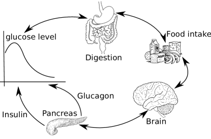
Figure 5: Glucose metabolism

We will focus on the assimilation of sweeteners: i.e., sugars or artificial sweeteners such as aspartame. Whenever we eat something sweet either natural or artificial, the sweet sensation sends a signal to the brain (through neurotransmitters) that in turns stimulates the production of insulin by pancreas. In the case of sugar, the digestion transforms food into nutrients (i.e., glucose) that are absorbed by blood. This way, sugar through digestion increases glucose in blood giving the sensation of satiety. In case the income of glucose produces hyperglycemia, the levels of glucose are promptly equilibrated by the intervention of insulin. Unlike sugar, artificial sweeteners are not assimilated by the body, hence they do not increase the glucose levels in blood. Nevertheless the insulin produced under the stimuli originated by the sweet sensation, although weak, can still cause the rate of glucose to drop engendering hypoglycemia. In response to that, the brain induces the stimulus of hunger. As a matter of fact this appears as an unwanted/toxic behaviour. Indeed the assimilation of food (even if it contains aspartame) should calm hunger and induce satiety not the opposite.

This schema suggests that we should consider four levels for glycemia: low, hunger, equilibrium and high. Likewise for insulin we assume three levels: inactive, low and high. All other actors involved in glucose regulation, have only two levels (inactive or active). In this example, duration do not play a fundamental role, for the sake of simplicity we have set all complementary activities such as production of insulin and glucagon, to take the same amount of time, the signal to the brain is the fastest, and the decay of glycemia values are much longer than the digestion process.

Thus the set of involved entities is

$$\mathcal{E}=\{Sugar,Aspartame,Glycemia,Glucagon,Insulin\}$$

and their expression levels and corresponding decays are:

$$\begin{array}[]{|lcl|}\hline\cr\mbox{levels}&&\mbox{duration}\\ \hline\cr\mathcal{L}_{sugar}=\{0,1\}&&\delta_{sugar}(1)=2\\ \hline\cr\mathcal{L}_{aspartame}=\{0,1\}&&\delta_{aspartame}(1)=2\\ \hline\cr\mathcal{L}_{glycemia}=\{0,1,2,3\}&&\delta_{glycemia}(1)=8\\ &&\delta_{glycemia}(2)=8\\ &&\delta_{glycemia}(3)=8\\ \hline\cr\mathcal{L}_{glucagon}=\{0,1\}&&\delta_{glucagon}(1)=3\\ \hline\cr\mathcal{L}_{insulin}=\{0,1,2\}&&\delta_{insulin}(1)=3\\ &&\delta_{insulin}(2)=3\\ \hline\cr\end{array}$$

The levels of glycemia are: 0 corresponding to low, 1 to hunger, 2 to equilibrium and 3 to high. Likewise for insulin we have 0 that corresponds to inactive, 1 to low and 2 to high. All levels for the other species are 0 for inactive and 1 for active.

The set of potential activities $\mathcal{P}=\{\alpha_{k}=A_{k};I_{k}\xrightarrow{}R_{k}\mid k\in[1..9]\}$ for the glucose metabolism example is:

$$\begin{array}[]{l l}\alpha_{1}:&(Sugar,1);\emptyset\xrightarrow{}(Insulin,+1),(Glycemia,+1)\\ \alpha_{2}:&(Aspartame,1);\emptyset\xrightarrow{}(Insulin,+1)\\ \alpha_{3}:&\emptyset;(Glycemia,1)\xrightarrow{}(Glucagon,+1)\\ \alpha_{4}:&(Glycemia,3);\emptyset\xrightarrow{}(Insulin,+1)\\ \alpha_{5}:&(Insulin,2);\emptyset\xrightarrow{}(Glycemia,-1)\\ \alpha_{6}:&(Insulin,1),(Glycemia,3);\emptyset\xrightarrow{}(Glycemia,-1)\\ \alpha_{7}:&(Insulin,1);(Glycemia,2)\xrightarrow{}(Glycemia,-1)\\ \alpha_{8}:&(Glucagon,1);\emptyset\xrightarrow{}(Glycemia,+1)\end{array}$$

$\alpha_{1}$ and $\alpha_{2}$ represent the assimilation of Sugar and Aspartame, respectively: while Aspartame only increases the level of Insulin, Sugar also increases Glycemia. $\alpha_{3}$ takes care of hypoglycemia, i.e., a Glycemia level equal to 0 (obtained by using $(Glycemia,1)$ as inhibitor) engenders the production of Glucagon. On the contrary, hyperglycemia causes the production of Insulin ($\alpha_{4}$). The presence of Insulin lowers Glycemia (activities $\alpha_{5},\alpha_{6},\alpha_{7}$). In particular Insulin level equal to 1 plays a role in the decrease of Glycemia only in case of hyperglycemia $\alpha_{6}$ or hypoglycemia $\alpha_{7}$, otherwise the signal is not strong enough and we need Insulin at level 2 to see the effect on Glycemia ($\alpha_{5}$). Last activity describes the role of Glucagon which if active increases the level of Glycemia.

For this example we consider an empty set of mandatory activities. Observe now the behaviour of $Glycemia$ in the following scenario:

$$\begin{array}[]{ll}\text{initial state}&\langle 3,0\rangle\\ \text{$8$ time units elapse, counter at level $3$ updates}&\langle 3,8\rangle\\ \text{one time unit elapses, $Glycemia$ decays}&\langle 2,0\rangle\\ \text{one time unit elapses, counter at level $2$ updates}&\langle 2,1\rangle\\ \text{activity $\alpha_{5}$ decreases $Glycemia$ level}&\langle 1,0\rangle\\ \text{$8$ time units elapse, counter at level $1$ updates}&\langle 1,8\rangle\\ \text{one time unit elapses, $Glycemia$ decays}&\langle 0,0\rangle\\ \text{one time unit elapses, no effect since $\delta_{glycemia}(0)=\omega$ \quad}&\langle 0,0\rangle.\end{array}$$

Figure 6 shows a simplified ANDy network $(\mathcal{E},\mathcal{P},\emptyset)$. The shown fragment focuses only on the activity schema linking inputs (i.e., activators and inhibitors) to results. Each input arc is labeled with either letter A or letter I denoting whether the input place is an activator or an inhibitor, respectively. Likewise, each output arc is labeled with a + or a - to denote increase or decrease of product levels by 1. For each activity transition $\alpha$, we have omitted place $q_{\alpha}$ and all arcs in the opposite direction. The numbers inside each transition refer to the corresponding activity. Figure 7, instead, shows a portion of the complete initially marked ANDy network focusing only on activity $\alpha_{7}$.

Figure 6: Simplified ANDy network of glucose metabolism.

Figure 7: A portion of the ANDy network of glucose metabolism with an initial marking.

The obtained network allows to simulate and intuitively confirm expected behaviours. In addition and as explained in previous section, we can perform exhaustive checks and for instance automatically verify the following CTL properties:

Symptoms:

Is it possible to have an anomalous decrease of glucose levels in blood (revealing hypoglycemia)?

$$\mathbf{E}\mathbf{F}(Glycemia,0)$$

Causality:

Does assimilation of sweeteners cause hypoglycemia?

$$\begin{array}[]{l}\mathbf{E}\mathbf{F}[((Sugar,1)\vee(Aspartame,1))\wedge(Glycemia,1)]\rightarrow\mathbf{A}\mathbf{F}(Glycemia,2)\end{array}$$

For this formula we highlight the different mode-of-action depending on the absorption of sugar or aspartame.

In the case of the assimilation of sugar, it induces an increase of the production of insulin and an augmentation of the blood glucose levels. Nonetheless the levels of insulin produced are not enough to cause the glycemia to drop and the formula is satisfied.

$$\begin{array}[]{l}(Sugar,1),(Aspartame,0),(Glycemia,1),(Insulin,0),(Glucagon,0)\xrightarrow{\alpha_{1}}\\ (Sugar,1),(Aspartame,0),\mathbf{(Glycemia,2)},(Insulin,1),(Glucagon,0)\end{array}$$

In the case of the assimilation of aspartame but not sugar, it causes only an increase of insulin. Unfortunately, this increment is sufficient to induce a decrease of blood glucose levels thus contradicting the formula above. This illustrates the toxic behaviour caused by aspartame.

$$\begin{array}[]{l}(Sugar,0),(Aspartame,1),(Glycemia,1),(Insulin,0),(Glucagon,0)\xrightarrow{\alpha_{2}}\\ (Sugar,0),(Aspartame,1),(Glycemia,1),(Insulin,1),(Glucagon,0)\xrightarrow{\alpha_{7}}\\ (Sugar,0),(Aspartame,0),\mathbf{(Glycemia,0)},(Insulin,1),(Glucagon,0)\end{array}$$

The ANDy network, its implementation in Snoopy and formulas for Charlie analyser as well as some results can be found in [15].

5 Related works

From a technical point of view, the closest related work is on reaction systems [1] or their Petri net representation [21]. Although we use a similar definition for activity, the semantics we have proposed is inherently different: in [1] all enabled reactions occur in one step while we consider two forms of activity evolution: simultaneous for mandatory activities and interleaved for potential ones. Furthermore, we have introduced discrete abstract levels that, to the best of our knowledge, are not taken into account in reaction systems. Also, we have presented a more elaborated notion of time that governs both entities and activities. In [22] the authors consider an extension of reaction systems with duration but it concerns only decay and not duration of activities. Furthermore the decay is referred to the number of steps and not to the discrete time progression as in our case.

From the Petri net modelling point of view, our representation of time is considerably different from the approaches traditionally used in time and timed Petri nets ([23] presents a survey with insightful comparison of the different approaches). The main difference lies on the fact that the progression of time is implicit and external to the system. By contrast, in our proposal we have assumed the presence of an explicit way of incrementing duration (modelled by synchronised counters). This is also different from the notion of timestamps introduced in [24] that again refers to an implicit notion of time. Indeed, our approach is conceptually closer to Petri nets with causal time [25] for the presence of an explicit transition for time progression. Nevertheless, in our approach time cannot be suspended under the influence of the environment (as is the case in [25]).

Time is featured also in [26] based on the Thomas framework and using delays as parameters to be discovered. A similar approach but based on timed automata is presented in [27] and [28]. In all these proposals, delays are reminiscent of our durations for mandatory activities but our semantics is more general as it includes the treatment of decay and potential activities.

In a broader sense, our work could also be related to P-systems [29, 30] or the $\kappa$-calculus [31] that describe the evolution of cells through rules. Both these approaches are mainly oriented to simulation while we are interested in verification aspects. Moreover, always related to the modelling in Petri nets but with a different aim, levels have been used in qualitative approaches to address problems related to the identification of steady states in genetic networks such as in [32]. Nevertheless these contributions abstract away from time related aspects that are instead central in our proposal. It is also interesting to notice that our formalism adds a new node in between timed and qualitative regions in the classification in [33].

6 Final remarks

We have introduced ANDy to model time-dependent activity-driven systems, which consist of a set of entities present in the environment at a given level. Entities can age as time passes by and their level is governed by a set of mandatory and potential activities with duration. The ANDy network is compact and provides an intelligible representation of the described activities. Moreover, it is easily scalable as the size of the network grows linearly with the number of added entities and activities and the rule-based architecture of guarantees a modular construction of the systems. We have shown that, despite the ability of modelling timed (thus infinite) systems, ANDy networks have finite state space.

Moreover we have discussed how toxicity problems can be addressed using our formalism. To the best of our knowledge this is the first attempt to give a general methodology, a systemic approach of toxicity analysis rather than a particular technique to verify them. We have exemplified our approach to toxicity on the blood glucose regulation example.

As the semantics of ANDy is given in terms of high-level Petri nets, ANDy networks can be easily used as overlay of existing implemented tools. We have prototyped a tool to simulate and build the state space of an ANDy network using the SNAKES toolkit and Snoopy/Charlie. The first results [15] are very positive, ANDy is particularly suited to describe biological systems, in particular regulatory networks and pathways whose formalisation is based on rules (activities).

We plan to develop the ANDy approach along several directions. We want to extend the decay function to arbitrary maps in $\mathcal{L}$. The problem is to generalise the notion of increase and decrease in a relevant way for the application. More structure can also be given to the notion of entity. Characterising an entity by several attributes (instead of only one level) raises the question of the causal relationships between these attributes and their update strategy. Another aspect that will be addressed in the future is to consider dynamic models where entities are created and deleted, as in [34]. Finally, it would certainly be interesting to find a systematic way for approximating stochastic rates into activities duration and decays.

Acknowledgements.

We thank the anonymous reviewers of PNSE and BioPPN 2014 for their comments on the very first version of this paper. We are grateful to M. Heiner, F. Pommereau, Y.-S. Le Cornec and A. Finkelstein for useful suggestions and discussions.

Appendix A Encoding into Timed Automata

In Section 2 we have hinted at the construction of a timed automaton coming directly from the marking graph of an ANDy network. Here we present another encoding that is syntax-driven which is not straightforward because of the management of mandatory rules. Unfortunately, even if the obtained automata is smaller, we cannot avoid it to be exponential at least in the number of activities. We conclude this section showing that the semantics of ANDy in terms of timed automata is equivalent to the semantics in terms of high-level Petri nets.

Timed automata.

A timed automaton is an annotated directed (and connected) graph, with an initial node and provided with a finite set of non-negative real variables called clocks. Nodes (called locations) are annotated with invariants (predicates allowing to enter or stay in a location). Arcs are annotated with guards, communication labels, and possibly with some clock resets. Guards are conjunctions of elementary predicates of the form $x\leavevmode\nobreak\ \mathit{op}\leavevmode\nobreak\ c$, where $\mathit{op}\in\{>,\geq,=,>,\leq\}$ where $x$ is a clock and $c$ a (possibly parameterised) positive integer constant. As usual, the empty conjunction is interpreted as true. The set of all guards and invariant predicates will be denoted by $G$.

Definition A.1

A timed automaton $\mathit{TA}$ is a tuple $(L,l^{0},X,\Sigma,\mathit{Arcs},\mathit{Inv})$, where

• $L$ is a set of locations with $l^{0}\in L$ the initial one, $X$ is the set of clocks,

• $\Sigma=\Sigma^{s}\cup\Sigma^{u}\cup\Sigma^{b}$ is a set of communication labels, where $\Sigma^{s}$ are synchronous, $\Sigma^{u}$ are synchronous and urgent, and $\Sigma^{b}$ are broadcast ones,

• $\mathit{Arcs}\subseteq L\times(G\cup\Sigma\cup R)\times L$ is a set of arcs between locations with a guard in $G$, a communication label in $\Sigma\cup\{\epsilon\}$, and a set of clock resets in $R=2^{X}$; for all $a\in\Sigma^{u}$, we require the guard to be $\mathbf{true}$;

• $\mathit{Inv}:L\rightarrow G$ assigns invariants to locations.

It is possible to define a synchronised product of a set of timed automata that work and synchronise in parallel. The automata are required to have disjoint sets of locations, but may share clocks and communication labels which are used for synchronisation. We define three communication policies:

• synchronous communications through labels $a\in\Sigma^{s}$ that require all the automata having label $a$ to synchronise on $a$;

• synchronous urgent communications through labels $u\in\Sigma^{u}$ that are synchronous as above but urgent meaning that there will be no delay if transition with label $u$ can be taken;

• broadcast communications through labels $b!,b?\in\Sigma^{b}$ meaning that a set of automata can synchronise if one is emitting; notice that, a process can always emit (e.g., $b!$) and the receivers ($b?$) must synchronise if they can.

The synchronous product $\mathit{TA}_{1}\parallel\ldots\parallel\mathit{TA}_{n}$ of timed automata, where for each $j\in[1,\ldots,n]$, $\mathit{TA}_{j}=(L_{j},l^{0}_{j},X_{j},\Sigma_{j},\mathit{Arcs}_{j},\mathit{Inv}_{j})$ and all $L_{j}$ are pairwise disjoint sets of locations is the timed automaton $\mathit{TA}=(L,l^{0},X,\Sigma,\mathit{Arcs},\mathit{Inv})$ such that:

• $L=L_{1}\times\ldots\times L_{n}$ and $l^{0}=(l^{0}_{1},\ldots,l^{0}_{n})$, $X=\bigcup_{j=1}^{n}X_{j}$, $\Sigma=\bigcup_{j=1}^{n}\Sigma_{j}$,

• $\forall l=(l_{1},\ldots,l_{n})\in L\colon\mathit{Inv}(l)=\bigwedge_{j}\mathit{Inv}_{j}(l_{j})$,

• $\mathit{Arcs}$ is the set of arcs $(l_{1},\ldots,l_{n})\stackrel{{\scriptstyle g,a,r}}{{\longrightarrow}}(l^{\prime}_{1},\ldots,l^{\prime}_{n})$ such that (where for each $a\in\Sigma^{s}\cup\Sigma^{u},S_{a}=\{j\mid 1\leq j\leq n,a\in\Sigma^{s}_{j}\cup\Sigma^{u}_{j}\}$): for all $1\leq j\leq n$, if $j\not\in S_{a}$, then $l_{j}^{\prime}=l_{j}$, otherwise there exist $g_{j}$ and $r_{j}$ such that $l_{j}\stackrel{{\scriptstyle g_{j},a,r_{j}}}{{\longrightarrow}}l_{j}^{\prime}\in E_{j}$; $g=\bigwedge_{j\in S_{a}}g_{j}$ and $r=\bigcup_{j\in S_{a}}r_{j}$.

The semantics of a synchronous product $\mathit{TA}_{1}\parallel\ldots\parallel\mathit{TA}_{n}$ is that of the underlying timed automaton $\mathit{TA}$ (synchronising on synchronous and broadcast communication labels) as recalled below, with the following notations. A location is a vector $l=(l_{1},\ldots,l_{n})$. We write $l[l^{\prime}_{j}/l_{j},j\in S]$ to denote the location $l$ in which the $j$th element $l_{j}$ is replaced by $l^{\prime}_{j}$, for all $j$ in some set $S$. A valuation is a function $\nu$ from the set of clocks to the non-negative reals. Let $\mathbb{V}$ be the set of all clock valuations, and $\nu_{0}(x)=0$ for all $x\in X$. We shall denote by $\nu\vDash F$ the fact that the valuation $\nu$ satisfies (makes true) the formula $F$. If $r$ is a clock reset, we shall denote by $\nu[r]$ the valuation obtained after applying clock reset $r\subseteq X$ to $\nu$; and if $d\in\mathbb{R}_{>0}$ is a delay, $\nu+d$ is the valuation such that, for any clock $x\in X$, $(\nu+d)(x)=\nu(x)+d$.

The semantics of a synchronous product $\mathit{TA}_{1}\parallel\ldots\parallel\mathit{TA}_{n}$ is defined as a timed transition system $(S,s_{0},\rightarrow)$, where $S=(L_{1}\times,\ldots\times L_{n})\times\mathbb{V}$ is the set of states, $s_{0}=(l^{0},\nu_{0})$ is the initial state, and $\rightarrow\subseteq S\times S$ is the transition relation defined by:

• (sync): $(\bar{l},\nu)\rightarrow(\bar{l^{\prime}},\nu^{\prime})$ if there exist arc $l\stackrel{{\scriptstyle g,a,r}}{{\longrightarrow}}l^{\prime}\in\mathit{Arcs}$ such that $\nu\vDash g$, $\nu^{\prime}=\nu[r]$, for $S_{a}=\{j\mid 1\leq j\leq n,a\in\Sigma^{s}_{j}\}$, $l^{\prime}=l[l^{\prime}_{j}/l_{j},j\in S_{a}]$, and there is no enabled transition with urgent communication label from $(\bar{l},\nu)$;

• (urgent): as (sync) but $a\in\Sigma^{u}$ and there is no delay if transition with urgent communication label can be taken;

• (broadcast): $(\bar{l},\nu)\rightarrow(\bar{l^{\prime}},\nu^{\prime})$ if there exist an output arc $l_{j}\stackrel{{\scriptstyle g_{j},b!,r_{j}}}{{\longrightarrow}}l_{j}^{\prime}\in\mathit{Arcs}_{j}$ and a (possibly empty) set of input arcs of the form $l_{k}\stackrel{{\scriptstyle g_{k},b?,r_{k}}}{{\longrightarrow}}l_{k}^{\prime}\in\mathit{Arcs}_{k}$ such that for all $k\in K=\{k_{1},\ldots,k_{m}\}\subseteq\{l_{1},\ldots,l_{n}\}\setminus\{l_{j}\}$, the size of $K$ is maximal, $\nu\vDash\bigwedge_{k\in K\cup\{j\}}g_{k}$, $l^{\prime}=l[l^{\prime}_{k}/l_{k},k\in K\cup\{j\}]$ and $\nu^{\prime}=\nu[r_{k},k\in K\cup\{j\}]$;

• (timed): $(l,\nu)\rightarrow(l,\nu+d)$ if $\nu+d\vDash\mathit{Inv}(l)$.

Here we exemplify timed automata usage: consider for instance the network of timed automata $\mathit{TA}_{1}$ and $\mathit{TA}_{2}$ with synchronous (non urgent) communications only:

whose behaviour is given by their synchronised product $\mathit{TA}_{1}\parallel\mathit{TA}_{2}$:

and where a possible run is:

Encoding into timed automata.

We are now ready to introduce the encoding of the high-level Petri net formalisation of ANDy, to this aim we need to add some notation:

Notation A.1

Let $\mathit{B}=\{\beta_{1},\ldots,\beta_{n}\}$ be the set of all mandatory activities identifiers from $\mathcal{M}$, ordered alphabetically, i.e., $\beta_{i}<\beta_{j}$ if $i<j$. We denote by

$$\mathit{B}^{\circledast}=\{seq(h)\mid h\in\mathcal{P}(\mathit{B})\wedge h\neq\emptyset\}\cup\{\varepsilon\},$$

the set of sequences $seq(h)$ obtained by concatenating the identifiers in non-empty subsets $h$ of $\mathit{B}$, where for each $h=\{\beta_{i_{1}},\ldots,\beta_{i_{m}}\mid\forall j,k:\leavevmode\nobreak\ i_{j}<i_{k}\}\in\mathcal{P}(\mathit{B})$, $seq(h)=\beta_{i_{1}}\cdots\beta_{i_{m}}$. We assume that if $\mathit{B}^{\circledast}=\{h_{1}\,.\,.\,h_{k}\}$, then the $h_{i}$’s are ordered by decreasing length and alphabetically in such a way that $h_{1}=\beta_{1}\cdots\beta_{|\mathit{B}|}$ and $h_{k}=\varepsilon$.

Moreover, $\beta_{i}=h[i]$ is the identifier at the $i$-position, and $h=h_{1}-h_{2}$ is the sequence of identifier in $h_{1}$ without those in $h_{2}$.

The encoding of an ANDy network is the synchronised product of one timed automaton for each entity in $\mathcal{E}$ together with a set of auxiliary automata that are used to handle potential and mandatory activities. The idea is that the global state of an ANDy network is divided into its local counterparts represented by state of entities (i.e., their levels). Thus for each entity $e$ we build a timed automaton $\mathit{TA}(e,\eta_{e})$ which has as many locations as the levels in $e$. Auxiliary automata are used to implement the encoding of places $p_{\rho}$ ($\mathit{TA}(\rho)$ for $\rho\in\mathcal{M}\cup\mathcal{P}$) and to realise time progression together with mandatory activities ($\mathit{TA}_{\surd}$). More formally:

Definition A.2

Given an ANDy network $(\mathcal{E},\mathcal{M},\mathcal{P})$, with initial expression level $\eta_{e}$ for each $e\in\mathcal{E}$, the corresponding timed automata encoding is

$$\llbracket(\mathcal{E},\mathcal{M},\mathcal{P})\rrbracket=\prod_{e\in\mathcal{E}}\mathit{TA}(e,\eta_{e})\parallel\prod_{\alpha\in\mathcal{P}}\mathit{TA}(\alpha)\parallel\prod_{\beta\in\mathcal{M}}\mathit{TA}(\beta)\parallel\mathit{TA}_{\surd}$$

where $\mathit{TA}(e,\eta_{e})$, $\mathit{TA}(\alpha)$,$\mathit{TA}(\beta)$ and $\mathit{TA}_{\surd}$ are defined next. In the following we assume $\mathit{B}$ to be the set of identifiers of mandatory activities in $\mathcal{M}$.

Entities.

$\mathit{TA}(e,\eta_{e})=(L_{e},l^{0}_{e},X_{e},\Sigma_{e},\mathit{Arcs}_{e},\mathit{Inv}_{e})$ where:

• $L_{e}=\{l^{e}_{i}\mid i\in[0\,.\,.\,\mathcal{L}_{e}]\}\cup\{k_{i}^{h},k_{i}^{d,h}\mid i\in[0\,.\,.\,\mathcal{L}_{e}],h\in\mathit{B}^{\circledast}\}$ with $l^{0}_{e}=l^{e}_{\eta_{e}}$

• $X_{e}=\{\lambda^{e}_{i},u^{e}_{i}\mid i\in[0\,.\,.\,\mathcal{L}_{e}]\}\cup\{x_{e}\}$

• $\Sigma^{s}_{e}=\{\alpha\mid\alpha\text{ identifier of an activity in }\mathcal{P}\}$, $\Sigma_{e}^{b}=\mathit{B}^{\circledast}$, $\Sigma_{e}^{u}=\{\surd h\mid h\in\mathit{B}^{\circledast}\}$

• $\mathit{Arcs}_{e}=\mathit{Arcs}_{\mathcal{P}}\cup\mathit{Arcs}_{\mathcal{M}}$ where

  $$\mathit{Arcs}_{\mathcal{P}}\!=\!\{l_{j}\xrightarrow{g(A_{\alpha})\wedge g(I_{\alpha})\wedge x_{e}=0,\alpha,r}l_{e}\mid e_{A_{\alpha}}\leq j<e_{I_{\alpha}},\alpha\in\mathcal{P},e\in A_{\alpha}\cup I_{\alpha}\cup R_{\alpha}\}$$

  with $j,e,e_{A_{\alpha}}$, and $e_{I_{\alpha}}$ are levels of $e$ defined as follows:

  $$e_{A_{\alpha}}=\begin{cases}\eta_{a}&\text{if }(e,\eta_{a})\in{A_{\alpha}}\\ 0&\text{otherwise}\end{cases}\qquad e_{I_{\alpha}}=\begin{cases}\eta_{i}&\text{if }(e,\eta_{i})\in{I_{\alpha}}\\ \mathcal{L}_{e}&\text{otherwise}\end{cases}$$

  $$g(A_{\alpha})=\begin{cases}\lambda^{e}_{\eta_{a}}\geq\Delta_{\alpha}&\text{if }(e,\eta_{a})\in A_{\alpha}\\ \mathbf{true}&\text{otherwise}\end{cases}\ g(I_{\alpha})=\begin{cases}\lambda^{e}_{\eta_{i}}\geq\Delta_{\alpha}&\text{if }(e,\eta_{i})\in I_{\alpha}\\ \mathbf{true}&\text{otherwise}\end{cases}$$

  $$m=\begin{cases}\max(0,\min(j+v,\mathcal{L}_{e}-1))&\text{if }(e,v)\in R_{\alpha}\\ j&\text{otherwise}\end{cases}$$

  $$r=\begin{cases}\emptyset&\text{if }(e,v)\not\in R_{\alpha}\\ \{u^{e}_{m},\}\cup\{\lambda_{x}^{e}\mid x\in[j+1,m]\}&\text{if }(e,v)\in R_{\alpha}\wedge m-j>0\\ \{u^{e}_{m},\}&\text{if }(e,v)\in R_{\alpha}\wedge m-j=0\\ \{u^{e}_{m},\}\cup\{\lambda_{x}^{e}\mid x\in[m+1,j]\}&\text{if }(e,v)\in R_{\alpha}\wedge m-j<0\end{cases}$$

  $$\begin{array}[]{ll}\mathit{Arcs}_{\mathcal{M}}=&\{l_{j}\xrightarrow{g(d)\wedge g,h?,\emptyset}k_{j}^{d,h},\mid j\in[0\,.\,.\,\mathcal{L}_{e}-1],h\in\mathit{B}^{\circledast}\}\ \cup\\ &\{l_{j}\xrightarrow{\neg g(d)\wedge g,h?,\emptyset}k_{j}^{h},\mid j\in[0\,.\,.\,\mathcal{L}_{e}-1],h\in\mathit{B}^{\circledast}\}\ \cup\\ &\{k_{j}^{d,h}\xrightarrow{\mathbf{true},h^{\prime},r\cup\{x_{e}\}}l_{e},\mid j\in[0\,.\,.\,\mathcal{L}_{e}-1],h,h^{\prime}\in\mathit{B}^{\circledast},h<h^{\prime}\}\ \cup\\ &\{k_{j}^{h}\xrightarrow{\mathbf{true},\surd h^{\prime},r^{\prime}\cup\{x_{e}\}}l_{e}^{\prime},\mid j\in[0\,.\,.\,\mathcal{L}_{e}-1],h,h^{\prime}\in\mathit{B}^{\circledast},h<h^{\prime}\}\end{array}$$

  where

  $$\begin{array}[]{lcl}g&=&\!\bigwedge_{k=1}^{n}g(\beta_{k})\wedge\bigwedge_{k=1}^{m}\neg g(\beta^{\prime}_{m})\text{ for }h=\beta_{1}\cdots\beta_{n}\text{ and }h_{1}-h=\beta^{\prime}_{1}\cdots\beta^{\prime}_{m}\\ g(\beta)&=&g^{\prime}(A_{\beta})\wedge g^{\prime}(I_{\beta})\text{ and }\beta=A_{\beta};I_{\beta}\xrightarrow{\Delta_{\beta}}R_{\beta}\\ g(d)&=&u_{j}>\delta_{e}(j)\end{array}$$

  $$g^{\prime}(A_{\beta})=\begin{cases}j\geq\eta_{a}\wedge\lambda^{e}_{\eta_{a}}\geq\Delta_{\beta}&\text{if }(e,\eta_{a})\in A_{\beta}\\ \mathbf{true}&\text{otherwise}\end{cases}$$

  $$g^{\prime}(I_{\beta})=\begin{cases}j<\eta_{i}\wedge\lambda^{e}_{\eta_{i}}\geq\Delta_{\beta}&\text{if }(e,\eta_{i})\in I_{\beta}\\ \mathbf{true}&\text{otherwise}\end{cases}$$

  $$\begin{array}[]{lcl}m&=&\max(0,\min(\sum_{i\in[1\,.\,.\,n]}f(h[i]^{\prime})+j-1,\mathcal{L}_{e}-1))\\ m^{\prime}&=&\max(0,\min(\sum_{i\in[1\,.\,.\,n]}f(h[i]^{\prime})+j,\mathcal{L}_{e}-1))\\ &&\mbox{ where }f(h[i])=\begin{cases}v&\text{if }(e,v)\in R_{\beta_{i}}\\ 0&\text{otherwise}\end{cases}\end{array}$$

  $$\begin{array}[]{ll}r=&\begin{cases}\{u^{e}_{m}\}\cup\{\lambda_{x}^{e}\mid x\in[j+1,m]\}&\text{if }m-j>0\\ \{u^{e}_{m}\}&\text{if }m-j=0\\ \{u^{e}_{m}\}\cup\{\lambda_{x}^{e}\mid x\in[m+1,j]\}&\text{if }m-j<0\end{cases}\\ r^{\prime}=&\begin{cases}\{u^{e}_{m^{\prime}}\}\cup\{\lambda_{x}^{e}\mid x\in[j+1,m^{\prime}]\}&\text{if }m^{\prime}-j>0\\ \{u^{e}_{m^{\prime}}\}&\text{if }e\in h^{\prime}\wedge m^{\prime}-j=0\\ \{u^{e}_{m^{\prime}}\}\cup\{\lambda_{x}^{e}\mid x\in[m^{\prime}+1,j]\}&\text{if }m^{\prime}-j<0\\ \emptyset&\text{if }e\notin h^{\prime}\end{cases}\end{array}$$

  where $e\in h$ denotes formula: $\exists\beta_{k}=A_{\beta_{k}};I_{\beta_{k}}\xrightarrow{\Delta_{\beta_{k}}}R_{\beta_{k}}$ s.t. $h=\beta_{1}\cdots\beta_{n},1\leq k\leq n\wedge(e,v)\in R_{\beta_{k}}$

• $Inv_{e}(l^{e}_{i})=u^{e}_{i}\leq\delta_{e}(i)$ for all $i\in[0\,.\,.\,\mathcal{L}_{e}]$

Potential activity.

$\mathit{TA}(\alpha)=(L_{\alpha},l^{0}_{\alpha},X_{\alpha},\Sigma_{\alpha},\mathit{Arcs}_{\alpha},\mathit{Inv}_{\alpha})$ for $\alpha\in\mathcal{P}$ where

• $L_{\alpha}=\{l_{\alpha}\}$, $l^{0}_{\alpha}=\alpha$, $X_{\alpha}=\{w_{\alpha}\}$, $\Sigma^{s}_{\alpha}=\{\alpha\}$

• $\mathit{Arcs}_{\alpha}=\{l_{\alpha}\xrightarrow{w_{\alpha}\geq\Delta_{\alpha},\alpha,\{w_{\alpha}\}}l_{\alpha}\}$

• $\mathit{Inv}_{\alpha}(l_{\alpha})=\mathbf{true}$.

Mandatory activity.

$\mathit{TA}(\beta)=(L_{\beta},l^{0}_{\beta},X_{\beta},\Sigma_{\beta},\mathit{Arcs}_{\beta},\mathit{Inv}_{\beta})$ for $\beta\in\mathcal{M}$ where

• $L_{\beta}=\{l_{\beta},l^{\prime}_{\beta}\}$, $l^{0}_{\beta}=l_{\beta}$, $X_{\beta}=\{w_{\beta}\}$, $\Sigma_{\beta}^{b}=\mathit{B}^{\circledast}$, $\Sigma_{\beta}^{u}=\{\surd h\mid h\in\mathit{B}^{\circledast}\}$

• $\mathit{Arcs}_{\beta}=\{l_{\beta}\xrightarrow{w_{\beta}\geq\Delta_{\beta},h?,\emptyset}l^{\prime}_{\beta}\mid h\in\mathit{B}^{\circledast},\beta\in h\}\cup\{l^{\prime}_{\beta}\xrightarrow{\mathbf{true},\surd h,\{w_{\beta}\}}l^{\prime}_{\beta}\mid h\in\mathit{B}^{\circledast},\beta\in h\}$

• $\mathit{Inv}_{\beta}(l_{\beta})=\mathbf{true}$ and $\mathit{Inv}_{\beta}(l^{\prime}_{\beta})=\mathbf{true}$.

Time.

$\mathit{TA}_{\surd}=(L_{\surd},l^{0}_{\surd},X_{\surd},\Sigma_{\surd},\mathit{Arcs}_{\surd},\mathit{Inv}_{\surd})$ where

• $L_{\surd}=\{l_{h}\mid h\in\mathit{B}^{\circledast}\}\cup\{l_{\bot}\}$, $l^{0}_{\surd}=l_{h_{1}}$, $X_{\surd}=\{x\}$, $\Sigma_{\surd}^{b}=\mathit{B}^{\circledast}$, $\Sigma_{\surd}^{u}=\{\surd h\mid h\in\mathit{B}^{\circledast}\}$

• $\mathit{Arcs}_{\surd}=\begin{array}[]{l}\{l_{h_{i}}\xrightarrow{x=1,h_{i}!,\emptyset}l_{h_{i}+1},l_{h_{i}+1}\xrightarrow{\mathbf{true},\surd h_{i},\{x\}}l_{h_{1}}\mid h,i\in[1\,.\,.\,n-1]\}\\ \cup\ \{l_{h_{n}}\xrightarrow{x=1,h_{n}!,\emptyset}l_{\bot},l_{\bot}\xrightarrow{\mathbf{true},\surd\varepsilon,\{x\}}l_{h_{1}}\}\end{array}$

• $\mathit{Inv}_{\surd}(l)=\mathbf{true}$ for all $l\in L_{\surd}$.

Theorem A.3

The above encoding of ANDy network $(\mathcal{E},\mathcal{M},\mathcal{P})$ is correct and complete.

Proof A.4 (Sketch)

Follows by induction on the length of the run and from a case analysis on the transition performed.

Some intuitions on the proof follows. For each entity $e$, the corresponding marking of place $p_{e}$, $M(p_{e})=\langle l_{e},u_{e},\lambda_{e}\rangle$, in the Petri net representation is encoded by the state (location $l^{e}_{l_{e}}$ and valuations of clocks variables $u^{e}_{l_{e}},\lambda^{e}_{i}$ for $i\in[0\,.\,.\,\mathcal{L}_{e}-1]$) of each timed automaton $\mathit{TA}(e,\eta_{e})$. Marking of places $p_{\rho}$ (for $\rho\in\mathcal{M}\cup\mathcal{P}$) is given by the valuation of clock $w_{\rho}$ in the corresponding timed automaton $\mathit{TA}(\rho)$.

Each transition of the Petri net is encoded by (a series of) timed automata arcs. For each transition $t_{\alpha}$ (corresponding to potential activity $\alpha$) involving $e$ there is a (synchronous) arcs in the timed automaton $\mathit{TA}(e,\eta_{e})$ whose guard describes its role in the activity (activator, inhibitor or result). Clock $w_{\alpha}$ in $\mathit{TA}(\alpha)$ implements the constraint that the activity $\alpha$ is performed at most once in the interval $\Delta_{\alpha}$: $w_{\alpha}\geq\Delta_{\alpha}$. This way, the synchronous product of all automata reconstructs the full guard of the activity $\alpha$ and exactly one transition in the synchronised product of automata corresponds to the firing of transition $t_{\alpha}$. The state reached after this transition coincides with the corresponding marking in the Petri net.

Transition $t_{c}$ is trickier as time progression causes decay but more importantly the simultaneous action of mandatory activities. Notice that mandatory activities concern the global state of an ANDy network (the maximal set of enabled mandatory activities has to be performed each time $t_{c}$ fires) but each sub-automaton of the synchronised automaton as only a partial/local information. That is why, we need to introduce the auxiliary automaton $\mathit{TA}_{\surd}$ that coordinates and gathers partial information from all other automata. Thus, the implementation of $t_{c}$ has two phases. The first one gathers partial information, performs the selection of the largest set of enabled mandatory activities and forces the time to progress in a discrete fashion; the second phase completes the time progression and synchronises all timed automata communicating the chosen maximal set of mandatory activities. Both phases are initiated by automaton $\mathit{TA}_{\surd}$ which has two types of arcs: broadcast ones for the first phase and urgent synchronous ones for the second (see Figure 8).

Figure 8: The shape of timed automaton $\mathit{TA}_{\surd}$ for $\mathit{B}^{\circledast}=\{\beta_{1}\beta_{2},\beta_{1},\beta_{2},\epsilon\}$, where $\surd\beta_{1}\beta_{2}$, $\surd\beta_{1}$, $\surd\beta_{2}$, $\surd\epsilon$ are all synchronous urgent communication labels.

More precisely, $\mathit{TA}_{\surd}$ progressively interrogates the entities timed automata $\mathit{TA}(e,\eta_{e})$ and the mandatory activities automata $\mathit{TA}(\beta_{i})$ to “compute” for each automaton the maximal set of enabled mandatory activities. This is obtained through broadcast arcs labelled with sequences of mandatory activities identifiers $h\in\mathit{B}^{\circledast}$, from the longest ($h=seq(\mathit{B})=\beta_{1}\cdots\beta_{n}$) to the shortest ($h=\epsilon$, i.e., no mandatory activity is enabled). As broadcast is a non blocking transition and because of the ordering on sequences in $\mathit{B}^{\circledast}$, each entity automaton chooses its maximal set of mandatory activities it is involved in. If it is necessary, it also performs decay. When all automata $\mathit{TA}(e,\eta_{e})$ and $\mathit{TA}(\beta_{i})$ have agreed on some sequence $h=\beta_{i_{1}}\,.\,.\,\beta_{i_{m}}$ (in the worst case $h$ is empty) the first phase is completed and $\{\beta_{i_{1}},\,.\,.\,,\beta_{i_{m}}\}$ is the largest set of enabled mandatory activities. The second phase is then implemented with an urgent synchronous arc synchronising all automata: $\mathit{TA}_{\surd}$, $\mathit{TA}(e,\eta_{e})$, for each $e\in\mathcal{E}$, and $\mathit{TA}(\beta_{i})$, for $i\in[i_{1}\,.\,.\,i_{m}]$. Notice that guards on broadcast transitions constraint the clocks to progress by one time unit at once. As a consequence, at the end of the two phase algorithm, timed automata of entities and of places $p_{\rho}$ together with the corresponding clocks valuations exactly encode the marking reached after firing $t_{c}$.

References

- [1] Brijder R, Ehrenfeucht A, Main MG, Rozenberg G. A Tour of reaction Systems. Journal of Foundations of Computer Science. 2011;22(7):1499–1517.
- [2] Wang F. Formal verification of timed systems: A survey and perspective. In: Proceedings of the IEEE; 2004. p. 1–23.
- [3] Alon U. An introduction to systems biology: design principles of biological circuits. CRC press; 2006.
- [4] Baldan P, Cocco N, Marin A, Simeoni M. Petri nets for modelling metabolic pathways: a survey. Natural Computing. 2010;9(4):955–989.
- [5] Thomas R. Boolean formalisation of genetic control circuits. Journal of theoretical biology. 1973;42:565–583.
- [6] Cardelli L. Abstract Machines of Systems Biology. Transactions on Computational Systems Biology. 2005;3737:145–168.
- [7] Giavitto JL, Malcolm G, Michel O. Rewriting systems and the modelling of biological systems. Comparative and Functional Genomics. 2004 Feb;5:95–99.
- [8] Waters MD, Fostel JM. Toxicogenomics and systems toxicology: aims and prospects. Nature reviews Genetics. 2004 Dec;5(12):936–48.
- [9] Foster WR, Chen SJ, He A, Truong A, Bhaskaran V, Nelson DM, et al. A retrospective analysis of toxicogenomics in the safety assessment of drug candidates. Toxicologic pathology. 2007 Aug;35(5):621–35.
- [10] Serrano L. Synthetic biology: promises and challenges. Molecular Systems Biology. 2007;3(158).
- [11] Di Giusto C, Klaudel H, Delaplace F. Systemic approach for toxicity analysis. In: Proceedings of the 5th International Workshop on Biological Processes & Petri Nets. vol. 1159 of CEUR Workshop Proceedings. CEUR-WS.org; 2014. p. 30–44.
- [12] Pommereau F. Quickly prototyping Petri nets tools with SNAKES. Petri net newsletter. 2008 10;(10-2008):1–18. SNAKES is available here.
- [13] Heiner M, Herajy M, Liu F, Rohr C, Schwarick M. Snoopy - A Unifying Petri Net Tool. In: Petri Nets. vol. 7347 of LNCS. Springer; 2012. p. 398–407.
- [14] Heiner M, Schwarick M, Wegener J. Charlie – an extensible Petri net analysis tool. In: Devillers R, Valmari A, editors. Proc. PETRI NETS 2015. vol. 9115 of LNCS. Springer; 2015. p. 200–211.
- [15] Additional material;. Available from: http://prova.
- [16] Elowitz M, Leibler S. A Synthetic Oscillatory Network of Transcriptional Regulators. Nature. 2000;403(6767):335–8.
- [17] Jensen K. Coloured Petri Nets - Basic Concepts, Analysis Methods and Practical Use - Volume 1. EATCS Monographs on TCS. Springer; 1992.
- [18] Alur R, Dill DL. A Theory of Timed Automata. TCS. 1994;126(2):183–235.
- [19] De Cristofaro M, Daniels K. Toxicogenomics in Biomarker Discovery. In: Essential Concepts in Toxicogenomics. vol. 460 of Methods in Molecular Biology. Humana Press; 2008. p. 185–194.
- [20] Imlay J, Linn S. DNA damage and oxygen radical toxicity. Science. 1988;240(4857):1302–1309.
- [21] Kleijn J, Koutny M, Rozenberg G. Modelling Reaction Systems with Petri Nets. In: BioPPN-2011; 2011. p. 36–52.
- [22] Brijder R, Ehrenfeucht A, Rozenberg G. Reaction Systems with Duration. In: Computation, Cooperation, and Life. vol. 6610 of LNCS. Springer; 2011. p. 191–202.
- [23] Cerone A, Maggiolo-Schettini A. Time-Based Expressivity of Time Petri Nets for System Specification. TCS. 1999;216(1-2):1–53.
- [24] Hanisch HM, Lautenbach K, Simon C, Thieme J. Timestamp Petri Nets in Technical Applications. In: WODES ’98; 1998. p. 321–326.
- [25] Thanh CB, Klaudel H, Pommereau F. Petri nets with causal time for system verification. ENTCS. 2002;68(5):85–100.
- [26] Comet J, Bernot G, Das A, Diener F, Massot C, Cessieux A. Simplified Models for the Mammalian Circadian Clock. In: CSBio 2012. vol. 11 of Procedia Computer Science. Elsevier; 2012. p. 127–138.
- [27] Batt G, Salah RB, Maler O. On Timed Models of Gene Networks. In: Raskin J, Thiagarajan PS, editors. FORMATS 2007. vol. 4763 of LNCS. Springer; 2007. p. 38–52.
- [28] Siebert H, Bockmayr A. Incorporating Time Delays into the Logical Analysis of Gene Regulatory Networks. In: CMSB 2006,. vol. 4210 of LNCS. Springer; 2006. p. 169–183.
- [29] Paun A, Paun M, Rodríguez-Patón A, Sidoroff M. P Systems with proteins on Membranes: a Survey. Int Journal of Foundations of Computer Science. 2011;22(1):39–53.
- [30] Kleijn J, Koutny M. Membrane Systems with Qualitative Evolution Rules. Fundam Inform. 2011;110(1-4):217–230.
- [31] Danos V, Laneve C. Formal molecular biology. TCS. 2004;325(1):69–110.
- [32] Chaouiya C, Naldi A, Remy E, Thieffry D. Petri net representation of multi-valued logical regulatory graphs. Natural Computing. 2011;10(2):727–750.
- [33] Heiner M, Gilbert D. How Might Petri Nets Enhance Your Systems Biology Toolkit. In: Petri Nets. vol. 6709 of LNCS. Springer; 2011. p. 17–37.
- [34] Giavitto JL, Klaudel H, Pommereau F. Integrated regulatory networks (IRNs): Spatially organized biochemical modules. TCS. 2012;431(1):219–234.