NCTS-TH/1607

The Thermal Bath of de Sitter from Holography

Chong-Sun Chu^1,2, Dimitrios Giataganas¹

¹ Physics Division, National Center for Theoretical Sciences,
National Tsing-Hua University, Hsinchu, 30013, Taiwan
² Department of Physics, National Tsing-Hua University, Hsinchu 30013, Taiwan

cschu@phys.nthu.edu.tw , dgiataganas@phys.cts.nthu.edu.tw

We consider the AdS/dS CFT correspondence and study the nature of the thermal bath of the de Sitter field theory using holography. Unlike the temperature of a thermal field theory in flat spacetime, the temperature of a superconformal field theory on de Sitter space is an integral part of the theory and leaves intact the conformal symmetry and supersymmetry. In the dual AdS side, there is no black hole. Instead we have cosmological expansion of the de Sitter factor. We consider a number of different observables, such as the entanglement entropy, two point correlation function, Wilson loops corresponding to static and spinning mesons in the field theory, and study their thermal properties using holography. The former two quantities have trivial temperature dependence due to conformal symmetry. We compute the energy of the quark anti-quark bound state for a static meson, as well as the energy and the angular momentum for a spinning meson. We find that there is a maximum distance, as well as a maximum spin for the latter case, beyond which the bound state become unstable. The temperature behavior of the physical quantities in these meson systems are similar to that of the usual thermal field theory with holographic black hole dual. With these examples, we show clearly how the field theory observables get their thermal properties from the bulk despite the absence of a black hole, with the role of the black hole horizon played by the cosmological expansion of the de Sitter factor of the AdS metric.

1 Introduction

de Sitter spacetime is an important background in cosmology because it not only describes the late time cosmology, but it is also crucial to the description of the inflationary early universe. In certain approximation, one may decouple quantum gravity and consider the quantum dynamics of other fields on a background de Sitter spacetime. Using perturbative quantum field theory on de Sitter space [1], one could connect of cosmological perturbation of the CMB in terms of the quantum fluctuation of the field theory in a slow roll potential. Among other things, the prediction of a scale invariant spectrum is in excellent agreement with the observational results of CMB and marked a remarkable success for the inflationary scenario. Nevertheless the picture suffers from the $\eta$ problem for the inflaton mass. Minimally coupled massless scalar field also suffers from large secular infrared effects and it would be nice to have better nonperturbative techniques to deal with them, beyond the often practiced approximation methods such as dynamical renormalization group (dRG) [2] or stochastic analysis [3].

Recently, by employing a specific dS-slicing coordination of the AdS space, a duality between type IIB string theory on AdS${}_{5}\times$S⁵ with dS₄ boundary and the ${\cal N}=4$ maximal superconformal Yang-Mills theory (SCYM) has been proposed [4]. It should be mentioned that while it is not possible to construct global supersymmetric field theory on four dimensional de Sitter spacetime [5, 6], the employment of global superconformal symmetry makes it possible. The Lagrangian of the SCYM theory has been constructed in [7]. See also [8]-[15] for related works. The SCYM theory is a cousin of the ${\cal N}=4$ supersymmetric Yang-Mills theory on flat space and, based on the holographic duality, it has been argued that SCYM theory would also share certain remarkable properties like its cousin, such as exact conformality, $SL(2,Z)$ strong-weak duality and integrability in some of its sectors. This makes the studies of the quantum ${\cal N}=4$ SCYM field theory a well motivated problem and it will be the subject of a different paper.

Here we simply mention that the de Sitter field theory has a finite temperature $T=H/(2\pi)$ due to Hawking radiation in de Sitter space. However this temperature has properties quite different from that of a thermal field theory in flat spacetime: 1. While ordinary temperature break Poincare supersymmetry, the de Sitter temperature does not break de Sitter superconformal symmetry. This is partially because the de Sitter temperature is not a independent parameter but is fixed directly in terms of the de Sitter space. 2. In terms of holography, the thermal vacuum of a quantum field theory in flat spacetime is dual to a black hole deep in the bulk. The presence of a black hole, in particular its horizon, changes the behavior of bulk supergravity solutions compared to the case without, and this is how the bulk gravitational dynamics could account for the properties of the thermal field theory. However there is no such black hole in our dual AdS spacetime. A motivation of this paper is to understand how the thermal properties of the de Sitter field theory is encoded in the bulk. It is natural to suspect that the role of the black hole horizon would be played by the cosmological expansion of the AdS bulk. We will demonstrate with examples that this is basically correct. Nevertheless the way the cosmological expansion affects the bulk solutions are different from the black hole horizon. In particular, in contrast with the effect of the AdS black hole where the presence of the gravitational attraction of the black hole pulls the string along the radial holographic direction, the cosmological expansion pulls the string in the directions orthogonal to the radial direction.

As said, the presence of de Sitter temperature is compatible with the superconformal symmetry of de Sitter space. As the two and 3-points correlation functions of the theory are completely fixed by the conformal symmetry, this means they depend on the temperature in a trivial way, through the geodesic distance of the space. This is indeed what we found in [4] using the bulk-to-boundary formalism. However this is not the case for other more nontrivial observables. For example, if we consider a Wilson loop operator $W_{C}$ on the de Sitter field theory, the expectation value of the Wilson loop could depend nontrivially on dimensionless combinations such as $LT$ or $AT^{2}$, where $L(A)$ is the length (area) of the loop $C$. This is a highly nontrivial problem, especially in the strongly coupled regime. The analysis of such nontrivial temperature dependence in strongly coupled field theory in de Sitter space is another motivation of this paper. Notice that gauge/gravity duals in de Sitter where also studied in [16, 17, 18, 19, 20, 21, 22, 23, 24, 25, 26, 27, 28, 29, 30, 31, 32]

The plan of the paper is as follows. In section 2, we consider the computation of entanglement entropy in the de Sitter theory in arbitrary dimensions. For the 2 dimensional case, an exact analytic solution is possible. As a by-product, we use the result of the entanglement entropy to obtain the equal time two-point correlator function. The result agrees with the one fixed by conformal symmetry. In section 3, we set up a heavy quark bound state with constant inter-quark distance. We compute the energy of the system and find that it behaves similarly to those of a thermal field theory in a flat spacetime. We discuss in what ways the cosmological expansion and the black hole horizon differs in their effects on the bulk dynamics of strings. In section 4, we consider a spinning heavy quark bound state with constant inter-quark distance. We regularize the energy and the angular momenta using the Legendre transformed action. We find that there exist a maximum spin beyond which the bound state ceases to exist. This is similar to the behavior of the bound states in a finite temperature field theories in flat spacetime. Section 5 contains our conclusions and discussions.

2 Entanglement Entropy

In this section, we compute the entanglement entropy for a rectangular stripe on dS space using holography [33, 34]. With a dS-slicing, the metric of AdS space takes the form

$$ds^{2}_{AdS_{d+1}}=dz^{2}+\sinh^{2}Hzds^{2}_{dS_{d}}~{},\qquad ds^{2}_{dS_{d}}=\frac{1}{H^{2}\eta^{2}}{\left({-d\eta^{2}+dx_{i}^{2}}\right)}~{},$$ (1)

where $i=1,\cdots,d-1$, $H=1/R$. In this coordinate patch, the boundary of the AdS space is located at $z=z_{\rm bdy}=\infty$ and is given by a $d$-dimensional de Sitter space. We consider a rectangular strip $\Sigma$ on the dS space described by

$$-\frac{L}{2}\leq x_{1}\leq\frac{L}{2}~{},\qquad 0\leq x_{j}\leq L_{1}~{},\quad(j=2,\cdots,d-1)~{},$$ (2)

where $L$ is the width of the strip and $L_{1}\gg L$ so to ensure translational invariance along the $x_{j}$ space directions. To obtain the entanglement entropy, we need to compute the area of the codimension 2 minimal surface $\gamma_{\Sigma}$ whose boundary is given by $\Sigma$. It turns out sufficient to consider a static parametrization of the surface

$$x_{1}=\sigma~{},\qquad x_{j}=\sigma_{j}~{},\qquad z=z{\left({\sigma}\right)}~{},\qquad\eta=\eta{\left({\sigma}\right)}~{}.$$ (3)

The boundary condition at $\sigma=\pm L/2$ is

$$z{\left({-\frac{L}{2}}\right)}=z{\left({\frac{L}{2}}\right)}=z_{\rm bdy}~{}.$$ (4)

We remark that the metric (1) belongs to a more general class of bulk metric of the form

$$ds^{2}=g_{\eta\eta}{\left({\eta,z}\right)}d\eta^{2}+\sum_{i=1}^{d-1}g_{ii}{\left({\eta,z}\right)}dx_{i}^{2}+g_{\rho\rho}{\left({\eta,z}\right)}dz^{2}~{},$$ (5)

where one can set up the computation of the minimal surface in an uniform manner . The entanglement entropy of the chosen region (3) is given by

$$4G_{N}^{(d+1)}S={\rm Area}(\gamma_{\Sigma})=L_{1}^{d-2}\int d\sigma A{\left({\sigma}\right)}\sqrt{D}~{},$$ (6)

where

$$A:=\sqrt{g_{22}g_{33}\ldots g_{dd}}~{},\qquad D:=g_{11}+g_{zz}z^{\prime 2}+g_{\eta\eta}\eta^{\prime 2}~{}.$$ (7)

The Hamiltonian is a constant of motion, since there is no explicit $\sigma$ dependence. Setting it equal to $-c$ we obtain the constraint

$$\frac{Ag_{11}}{\sqrt{D}}=c~{},$$ (8)

which gives a first order ordinary differential equation of $z$ and $\eta$

$$g_{zz}z^{\prime 2}+g_{\eta\eta}\eta^{\prime 2}+g_{11}\frac{c^{2}-A^{2}g_{11}}{c^{2}}=0~{}.$$ (9)

The other two equations of motion are obtained by the variation of the action (6) and gives

$$\sqrt{D}\partial_{\alpha}A+\frac{A}{2\sqrt{D}}{\left({\partial_{\alpha}g_{11}+\partial_{\alpha}g_{zz}\,z^{\prime 2}+\partial_{\alpha}g_{\eta\eta}\,\eta^{\prime 2}}\right)}-\begin{cases}\partial_{\sigma}{\left({\frac{A}{\sqrt{D}}g_{zz}z^{\prime}}\right)}=0~{},\\ \partial_{\sigma}{\left({\frac{A}{\sqrt{D}}g_{\eta\eta}\eta^{\prime}}\right)}=0~{},\end{cases}$$ (10)

where $\partial_{\alpha}=\partial_{\eta}$ or $\partial_{z}$. Eliminating the square root using the constraint (8), we obtain

$$\frac{g_{11}}{2c}\partial_{\alpha}(A^{2})+\frac{c}{2g_{11}}{\left({\partial_{\alpha}g_{11}+\partial_{\alpha}g_{zz}\,z^{\prime 2}+\partial_{\alpha}g_{\eta\eta}\,\eta^{\prime 2}}\right)}+\begin{cases}-c\partial_{\sigma}{\left({\frac{g_{zz}}{g_{11}}}\right)}z^{\prime}-c\frac{g_{zz}}{g_{11}}z^{\prime\prime}=0~{}.\\ -c\partial_{\sigma}{\left({\frac{g_{\eta\eta}}{g_{11}}}\right)}\eta^{\prime}-c\frac{g_{\eta\eta}}{g_{11}}\eta^{\prime\prime}=0~{}.\\ \end{cases}$$ (11)

The desired minimal surface $\gamma_{\Sigma}$ is obtained from solving the differential equations (8) and (11), subjected to the boundary conditions (4).

For the AdS_d+1 metric (1), the function (7) and the expressions appear in the equations of motion are

$$A(\sigma)={\left({\frac{\sinh Hz}{H\eta}}\right)}^{d-2}~{},\qquad\frac{g_{zz}}{g_{11}}=\frac{H^{2}\eta^{2}}{\sinh^{2}Hz}~{},\qquad\frac{g_{\eta\eta}}{g_{11}}=-1~{}.$$ (12)

Then the Hamiltonian constraint (8) and the equations of motion (11) take the relatively compact form

$$z^{\prime 2}-\frac{\sinh^{2}Hz}{H^{2}\eta^{2}}\eta^{\prime 2}+\frac{\sinh^{2}Hz}{H^{2}\eta^{2}}{\left({1-\frac{1}{c^{2}}\left(\frac{\sinh^{2}Hz}{H^{2}\eta^{2}}\right)^{d-1}}\right)}=0~{},$$ (13)

$$z^{\prime\prime}-2H\coth(Hz)\,z^{\prime 2}+\frac{2}{\eta}z^{\prime}\eta^{\prime}+\frac{\sinh(2Hz)}{2H\eta^{2}}\eta^{\prime 2}-\frac{\sinh(2Hz)}{2H\eta^{2}}{\left({1+\frac{d-2}{c^{2}}\left(\frac{\sinh^{2}Hz}{H^{2}\eta^{2}}\right)^{d-1}}\right)}=0~{},{}$$

(14)

$$\eta^{\prime\prime}+\frac{1}{\eta}\eta^{\prime 2}-\frac{1}{\eta}{\left({1+\frac{d-2}{c^{2}}\left(\frac{\sinh^{2}Hz}{H^{2}\eta^{2}}\right)^{d-1}}\right)}=0~{}.$$ (15)

In arbitrary number of dimensions the equations can be solved numerically. However, for the case of 2 dimensional conformal field theory, the factor $A{\left({\sigma}\right)}$ in (12) is equal to the unit and the equations of motion can be solved analytically.

2.1 Entanglement entropy for AdS₃/dS₂

Let us consider the case of a two dimensional conformal field theory. The equation of motion (15) for $\eta$ reads

$$\eta^{\prime\prime}+\frac{\eta^{\prime 2}}{\eta}-\frac{1}{\eta}=0~{}.$$ (16)

This has the solution

$$\eta=\pm\sqrt{\sigma^{2}+c_{1}\sigma+c_{2}}~{},$$ (17)

with $c_{1,2}$ being constants of integration. Notice that the solution of $\eta$ does not depend on the cosmological horizon $H$. Similarly the equation (14) gives

$$z^{\prime\prime}-2H\coth(Hz)z^{\prime 2}+\frac{2}{\eta}z^{\prime}\eta^{\prime}-\sinh(2Hz)\frac{1-H^{2}\eta^{\prime 2}}{2H\eta^{2}}=0~{}$$ (18)

and by substituting the solution (17), we get an second order differential equation for $z{\left({\sigma}\right)}$

$$z^{\prime\prime}-2H\coth(Hz)\,z^{\prime 2}+z^{\prime}\frac{2\sigma+c_{1}}{\sigma^{2}+c_{1}\sigma+c_{2}}+\sinh(2Hz)\frac{c_{1}^{2}-4c_{2}}{8H{\left({\sigma^{2}+c_{1}\sigma+c_{2}}\right)}^{2}}=0~{}.$$ (19)

The solution for $z$ then can be written in the compact form as

$$\coth Hz=\pm\frac{c_{3}}{4}\cdot\frac{4+c_{4}{\left({c_{1}^{2}-4c_{2}}\right)}\sigma}{\sqrt{c_{2}+c_{1}\sigma+\sigma^{2}}}~{},$$ (20)

where $c_{3}$ and $c_{4}$ are arbitrary integration constant. To specify the integration constants, we note that due to the symmetry of the problem, the geodesic should be left-right symmetric with respect to $x_{1}$. The geodesic has a turning point in the bulk $(z_{0},\eta_{0})$, which by the symmetry of the space, must therefore be located at $\sigma=0$, and the desired functions $z$ and $\eta$ must be even functions of $\sigma$. We obtain immediately that

$$\eta_{0}=\pm\sqrt{c_{2}}~{},\quad c_{1}=0~{},\quad c_{4}=0$$ (21)

and

$$\eta=\sqrt{\sigma^{2}+\eta_{0}^{2}}~{}.$$ (22)

In addition, $c_{3}$ can be expressed in terms of the turning point coordinates as

$$\coth^{2}Hz_{0}=\frac{c_{3}^{2}}{\eta_{0}^{2}}~{}.$$ (23)

Now the boundary condition (4) at $\sigma=\pm\frac{L}{2}$ gives

$$c_{3}^{2}=\frac{L^{2}}{4}+\eta_{0}^{2}~{}.$$ (24)

Therefore, eliminating $c_{3}$, we get the relation between the turning point $(z_{0},\eta_{0})$ and $L$:

$$\frac{\sinh^{2}Hz_{0}}{\eta^{2}_{0}}=\frac{4}{L^{2}}~{}.$$ (25)

Note that the Hamiltonian constraint (8) is satisfied by the solutions and applying it at the turning point for the geodesic it fixes the constant c as

$$c^{2}=\frac{4}{H^{2}L^{2}}~{}.$$ (26)

The minimized action is

$$4G_{N}^{(3)}S=\frac{2}{H}~{}\mbox{arctanh}\frac{2\sigma}{L}\bigg{|}_{0}^{L/2-\varepsilon}=R\log{\left({\frac{L}{\varepsilon}}\right)}~{},$$ (27)

where $R:=1/H$ is the radius of the AdS space and $\varepsilon\approx 0$ is a UV cutoff imposed in the $\sigma$ direction of the worldsheet. To compare with the field theory, we need to express (27) in terms of the UV cutoff of the field theory. This can be achieved by noting that if we introduce the radial coordinate $\rho$ of the bulk defined by

$$dz=R\frac{d\rho}{\rho}~{},$$ (28)

then the desired UV cutoff is given by

$$R\log\frac{1}{\epsilon}:=z{\left({{\frac{L}{2}-\varepsilon}}\right)}\simeq\frac{1}{2H}\log\frac{4\eta_{b}^{2}}{L\varepsilon}~{},$$ (29)

where

$$\eta_{b}:=\eta{\left({\frac{L}{2}}\right)}=\sqrt{\frac{L^{2}}{4}+\eta_{0}^{2}}~{},$$ (30)

is the time coordinate for the boundary point of the string. As a result,

$$4G_{N}^{(3)}S=2R\log\frac{L}{\epsilon\eta_{b}}~{}.$$ (31)

As $\eta_{b}$ should be treated as an independent parameter apart from $L$, we obtain [35, 36]

$$S=\frac{c}{3}\log\frac{L}{\epsilon}~{},\qquad c=\frac{3R}{2G_{N}^{(3)}}~{}.$$ (32)

The entropy (32) has a trivial $L$ dependence as fixed by conformal symmetry and has a trivial dependence on the de Sitter temperature. We also note that (32) is the same as the result in the flat space. This must be the case since the boundary metric is conformally related to that of the flat space and the logarithmic divergent piece is universal and depends trivially on the de Sitter temperature through the geodesic distance.

2.2 Two-Point Correlation Function

In the above computation of the holographic entanglement entropy, we have computed the length $L_{g}$ of the bulk geodesic joining the two points $x_{1}=\pm L/2$ on the boundary. As an application, this can be used to reconstruct the boundary correlation function for conformal operators. In general, for a scalar field of mass $m$ in the bulk of AdS₃, it has the lowest energy eigenvalue $H\Delta$ and the bulk propagator from $x$ to $x^{\prime}$ is given by

$$G(x,x^{\prime})=\int{\cal D}{\cal P}e^{-H\Delta L{\left({{\cal P}}\right)}},$$ (33)

where ${\cal P}$ is a path joining the two points and $L({\cal P})$ is the proper length of the path ${\cal P}$. In the semiclassical limit, the path integral is localized to its saddle points and is given by a sum over the geodesics. In the present case

$$G(x,x^{\prime})=e^{-H{\Delta}L_{g}}~{}.$$ (34)

According to [37, 38], (33) is also equal to the CFT correlator for the dual operator ${\cal O}$ in the large $N$ limit. Therefore we obtain in the large $N$ limit and semiclassical approximation the following expression for the two point function

$${\left<{{\cal O}{\left({x}\right)}{\cal O}{\left({x^{\prime}}\right)}}\right>}\simeq{\left({\frac{1}{\epsilon}}\right)}^{2\Delta}e^{-H\Delta L_{g}}~{},$$ (35)

where we have regulated the two point function by adopting a normalization involving an appropriate expression of the cutoff $\epsilon$. Using (31), we obtain

$${\left<{{\cal O}{\left({-\frac{L}{2},t}\right)}{\cal O}{\left({\frac{L}{2},t}\right)}}\right>}={\left({\frac{\eta_{b}}{L}}\right)}^{2\Delta}\sim\frac{1}{\sigma^{2\Delta}}~{},$$ (36)

where $\sigma$ is the de Sitter invariant distance

$$\sigma^{2}{\left({x,x^{\prime}}\right)}:=\frac{-{\left({\eta-\eta^{\prime}}\right)}^{2}+{\left({x-x^{\prime}}\right)}^{2}}{H^{2}\eta\eta^{\prime}}~{}.$$ (37)

(36) agrees with the result obtained in [4] using the bulk-to-boundary formalism. As the result is completely determined by conformal invariance, it is trivially depending on the de Sitter temperature through the geodesic distance.

3 Static Mesons in dS Theory

To see nontrivial dependence on temperature, let us introduce heavily massive external quarks and consider expectation value of the Wilson loop operators for space-like loop $C$ in the dS conformal field theory. According to holography [39, 40] they are determined in the large $N$ limit, by the minimal surface formed by the string world-sheet ending on the loop $C$ on the dS boundary. For convenience let us go to the planar coordinates for the dS space by setting $\eta=e^{-2Ht}$, we have

$$ds^{2}_{AdS_{d+1}}=dz^{2}+\sinh^{2}Hz~{}ds^{2}_{dS_{d}}~{},\qquad ds^{2}_{dS_{d}}=-dt^{2}+e^{2Ht}dx_{i}^{2}~{}.$$ (38)

3.1 The String Solution

We consider quark, anti-quark pair at the boundary (38) at

$$t=\tau~{},\qquad x_{1}=\pm\frac{L}{2}e^{-Ht}~{},$$ (39)

where the $\pm$ sign correspond to the positions of Q and Q̄ respectively. Note that in contrary to the flat space case, we have specified a specific time dependence for the position of the quarks, which give them a constant speed

$$v=\pm\frac{HL}{2}~{}.$$ (40)

pointing towards each other. This counter balance the expansion of the dS space and results in a constant $dS$ invariant distance (37) between the quarks

$$\sigma_{\rm inv}^{2}(Q,\bar{Q})=L^{2}~{}.$$ (41)

In other words, we have chosen here to consider meson of constant size and this is the closest analogy to the flat space case. Motivated by (39), we parametrize the string worldsheet as

$$t=\tau~{},\qquad x_{1}=e^{-Ht}\sigma~{},\qquad z=z(\sigma)~{}.$$ (42)

As we will see below, this parametrization guarantees time translation invariance for the Wilson loop and greatly simplifies the problem since the string world sheet is then govern by ordinary differential equations instead of partial differential equations. This is not the case if we have considered the usual static gauge parametrization $t=\tau,~{}x_{1}=\sigma,~{}z=z(\sigma)$, which does not satisfies the equations of motion.

It is not difficult to check that the Nambu-Goto (NG) action

$$S=\frac{\sqrt{\lambda}}{4\pi}\int d\sigma d\tau\sqrt{-g}~{},$$ (43)

for the parametrization (42) is consistent and gives only one non-trivial equation of motion

$$(1-H^{2}\sigma^{2})\sinh^{2}(Hz(\sigma))~{}z^{\prime\prime}(\sigma)-H^{2}\sigma(1-H^{2}\sigma^{2})~{}z^{\prime}(\sigma)^{3}{}$$

$$-\frac{3H}{2}(1-H^{2}\sigma^{2})\sinh(2Hz(\sigma))~{}z^{\prime}(\sigma)^{2}-2H^{2}\sigma\sinh^{2}(Hz(\sigma))~{}z^{\prime}(\sigma){}$$

$$-2H\cosh(Hz(\sigma))\sinh^{3}(Hz(\sigma))=0~{}.$$ (44)

The on-shell action takes the compact form

$$\frac{4\pi}{{\cal T}\sqrt{\lambda}}S=\int d\sigma\sinh Hz\sqrt{\sinh^{2}Hz+(1-H^{2}\sigma^{2})z^{\prime}(\sigma)^{2}}~{},$$ (45)

where we have integrated the world-sheet time to give a factor of ${\cal T}$. Notice that the resulting action is time independent reflecting the fact that the endpoints of the string have static invariant distance. For $H\sigma>1$ the action (45) may become zero or imaginary, this is a common characteristic for the orthogonal Wilson loop action in finite temperature field theories, where $H$ here plays the role of the black hole horizon.

The solution of the equation (44) can be found numerically and is presented in Figure (2). For small inter-quark distances $LH<<1$ the profile of the string has the usual U-shape of a hanging chain form with two fixed end-points. As the distance between the pair increases, the gravitational effects of the cosmological expansion in the interior of the AdS space give rises to a deformed U-shaped profile with more substantial modification around its turning point.

A couple of remarks are in order:

1. A common property of the holographic finite temperature field theories is that to each boundary distance of the string, there are two string solutions extending inside the bulk with different radial dependence [41, 42]. This is also the case here. As can be seen in Figure 2, there are two different string profiles in the bulk with different turning points $z_{0}$ for each boundary separation $L$. In Figure 2, we plot $L$ as a function of the turning point $z_{0}$. We find that for inter-quark distance less than a certain maximum, namely

$$L_{\rm max}H\simeq 0.92~{},$$ (46)

there always exists two different connected string solutions. At this point a natural question arises for the reason of the resemblance of our string solutions with the ones in the usual holographic thermal field theories. The mechanism that provides here twin world-sheets solutions is not because of the presence of a black hole in the bulk but is due to the expansion of the AdS space, an effect which is visible when the AdS metric is expressed in the form (1) in terms of the dS-sliced coordinates. Effectively, we have placed the string in the AdS space while keeping fixed the distance of the two boundary string endpoints by counterbalancing the expansion of the space with a given boundary velocity. However the rest of the string is still affected by the expansion, where the effect is enhanced as one goes deeper in the bulk. At some point the deformation of the connected string becomes so large that the string prefers energetically to break and become two separate strings and this is when the heavy quark bound state dissociates.

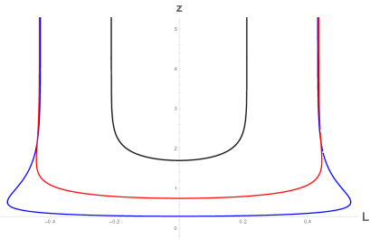
Figure 1: The string profile for different values of the inter-quark distance $L$. The boundary is at the large values of $z$. We plot string solutions with three different turning points $z_{0}$. The one with smallest $L$ has a string profile that is minimally deformed by the cosmological expansion. The other two string solutions correspond to the same inter-quark distance $L$, while the acceptable one has an endpoint closer to the boundary and is the energetically favorable. The string solution that goes deeper to the bulk, is clearly deformed by the cosmological expansion.

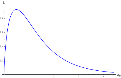
Figure 2: The inter-quark distance $L$ in units of $H$, in terms of the turning point $z_{0}$ of the string. For each value of $L$ there exist two string solutions with different turning points and energy. The acceptable one lies on the right branch of the maximum of the curve, since it has lower energy and it is stable. An example of such twin-solutions with the same boundary conditions is presented in Figure 2.

2. The deformation of the string in the bulk due to the cosmological expansion leads to a minor complication in the numerics . To obtain the string profile we solve the equation (44) by selecting the initial value of the holographic distance of the turning point of the world-sheet in the bulk $z_{0}$ and we shoot from this point towards the boundary. The selection of $z_{0}$ specifies the inter-quark distance $L$ at the boundary. For $\sigma=\sigma_{1}$ the string has a second turning point at $z_{1}=z(\sigma_{1})$, where $z^{\prime}(\sigma_{1})=\infty$ (Figure 2). At this point we need to invert the differential equation (44) to obtain the equation for $\sigma(z)$ and to shoot from the point $\sigma_{1}$ with initial conditions $\sigma(z_{1})=\sigma_{1}$ and $\sigma^{\prime}(z_{1})=0$. The two solutions can be combined to get the full profile of the string. Notice that we need the full solutions in order to find the energy of the string, where we integrate the energy density from $\sigma=\sigma_{0}$ to $\sigma=\sigma_{1}$ as a function of $\sigma$, and from $z_{1}$ to the boundary as a function of $z$. A series of such solutions are shown in Figure 4.

3. Notice that the deformation on the world-sheet due to the cosmological expansion is symmetric in the two edges. This is because we place the Q and Q̄ at equal distances from the origin $x_{1}=0$. Non-symmetric displacement of the pair along the $x_{1}$-axis leads to asymmetric deformation of the string world-sheet, enhanced on the side that is further away from the origin. A representative solution is shown in Figure 4.

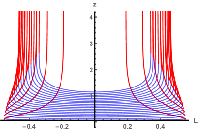
Figure 3: The string worldsheet for different values of the inter-quark distance $L$. We observe the changes on the solution as the turning point $z_{0}$ moves away from the boundary. In the bottom blue-colored region the derivatives $z^{\prime}{\left({\sigma}\right)}$ are finite, while the red-colored part includes the point of the infinite $z^{\prime}{\left({\sigma}\right)}$ derivative. Notice the string deformation enhancement as it goes closer to the bulk.

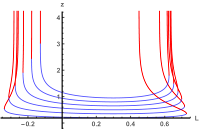
Figure 4: The heavy quark pair is located asymmetrically with respect to the origin. This asymmetry generates an asymmetric deformation of the bulk string, enhanced on the side that is further away from the origin, in this case at the right side. The midpoint of the string is at $\sigma_{0}H=0.3$.

3.2 The Energy of the Bound State

To obtain the energy of the bound state, one needs to regulate the on-shell Nambu-Goto action which is infinite due to the infinite length of the string world-sheet. Two subtraction schemes, the Legendre subtraction scheme and the mass subtraction scheme, have been widely used.

As the NG action is a functional of coordinates and the holographic direction of the string world-sheet satisfies a Neumann boundary condition, one needs to perform a Legendre transformation to change the boundary condition for the modified action. We point out that the Legendre transform is not diffeomorphic invariant; and for a successful canceling of the UV divergences, we should use the coordinate system $\rho$ (28) which is analogous to the AdS Poincare coordinates. The Legendre transform of the action in the $\rho$ coordinates is [45, 46]

$$S_{\rm Legendre}=\int d\tau\rho p_{\rho}\Big{|}^{\sigma\rightarrow\sigma_{2}}_{\sigma\rightarrow\sigma_{1}}~{},$$ (47)

where $\rho$ is the holographic direction, $p_{\rho}$ is the conjugate momentum

$$p_{\rho}=\frac{\delta S}{\delta(\partial_{\sigma}\rho)}~{},$$ (48)

and $\sigma_{1}$ and $\sigma_{2}$ are the endpoints of the string. Using the equation (28), we obtain $\rho p_{\rho}=p_{z}$, where

$$p_{z}=\frac{\delta S}{\delta(\partial_{\sigma}z)}~{}$$ (49)

is the conjugate momentum in the $z$ coordinate, and the desired Legendre term takes the form

$$\tilde{S}=S-\int d\tau p_{z}\Big{|}^{\sigma\rightarrow\sigma_{2}}_{\sigma\rightarrow\sigma_{1}}~{}.$$ (50)

The idea of the mass subtraction scheme is very intuitive. For the standard case of ${\cal N}=4$ SYM, a single heavy quark is the endpoint of a straight string that initiates from the boundary of the space ($z=\infty$) and goes into the bulk. The infinite mass of the quark is given by

$$M_{Q}=\int_{0}^{\infty}dz~{}.$$ (51)

The subtraction of this mass from the energy is equivalent to the subtraction using the Legendre term. For the finite temperature ${\cal N}=4$ SYM theory, the gravity dual has a black hole which introduces a lower bound on the holographic coordinate with a range $[z_{h},\infty)$, where $z_{h}$ is the position of the black hole. Then the corresponding mass for the heavy quark is given by

$$M_{Q}=\int_{z_{h}}^{\infty}dz~{}.$$ (52)

Note that apart from allowing to cancel the UV divergence of the NG action of the connected string worldsheet, $M_{Q}$ now also makes an IR contribution $z_{h}$, which is interpreted as a thermal contribution to the bound state energy. On the other hand in the Legendre term (50), information about the thermal properties of the horizon is present through the conjugate momentum and the string solution itself, however in a less direct manner. When computed at the boundary, the black hole contribution is negligible and the Legendre boundary term is equal to that of the zero temperature theory. In general, while both schemes offer the cancellation of the UV divergences, they could differ in their finite IR contribution and two schemes are not equivalent. The choice of regularization scheme depends on the problem and the physical quantity one desire to compute.

In the present case, due to its intuitive picture, one may want to use the mass subtraction scheme by subtracting out the energy of two single non-interacting quarks moving with the velocity (40). To do this, one needs an appropriate string solution with a single moving endpoint at the dS boundary

$$x_{0}=\tau~{},\qquad x_{1}=\frac{L}{2}e^{-Ht}~{}$$ (53)

with constant velocity. This is however not straightforward to find. In fact the most straightforward string world-sheet parametrization

$$x_{0}=\tau~{},\qquad x_{1}=\frac{L}{2}e^{-Ht}~{},\qquad z=z(\sigma)~{}$$ (54)

is not a solution of the full system of equations of motion, and a more involved string profile required. On the other hand, the Legendre subtraction can be performed without any problem. As a result, the regularized energy for our meson system is given by

$$E_{\rm tot}(L)=S_{Q\bar{Q}}-2S_{UV}~{},$$ (55)

where $S_{QQ}$ is given by the onshell action (45) and $S_{UV}$ is given by

$$\frac{4\pi}{{\cal T}\sqrt{\lambda}}S_{UV}=\sqrt{1-\frac{H^{2}L^{2}}{4}}\sinh Hz\Big{|}_{z\rightarrow\infty}~{},$$ (56)

where we have used the fact that our solution is independent of $\tau$ to integrate through the time to get an overall factor of ${\cal T}$. The factor of 2 accounts for the contribution from both endpoints. We have also used the fact that near the endpoints $\sigma=\pm L/2$, $z\to\infty$, the differential equation (44) is solved by

$$z^{\prime}=\mp\frac{1}{2HL}e^{2Hz},$$ (57)

where the sign $\mp$ is for $\sigma=\pm L/2$. As a result, near the boundary, $p_{z}$ is given by

$$p_{z}=\pm\sqrt{1-\frac{H^{2}L^{2}}{4}}\sinh Hz,$$ (58)

where the sign $\pm$ is for $\sigma=\pm L/2$. We remark that unlike the AdS case in the Poincare coordinates where the UV divergences of the Wilson loop do not depend on the spatial position of the string, in the present dS-sliced description of the AdS space where the metric becomes time dependent, the UV boundary term is multiplied by a factor that depends on the spatial position of the string. This is essential to cancel out the infinity.

Our result for $E_{\rm tot}(L)$ is plotted in Figure 5. The regularized energy of the bound state in the AdS/dS space has similarities with that of the bound state in the AdS black hole and the dual finite temperature ${\cal N}=4$ SYM field theory. The energy $E(L)$ has a turning point, indicating a maximum size of the heavy quark bound state with maximal energy for the state, beyond which it does not exist. Moreover, there exist two string solutions corresponding to the same size meson but have different energy. The acceptable solution is the one with the minimum energy which corresponds to the stable and energy preferred state. This resembles the known holographic results of finite temperature field theories including a black hole horizon.

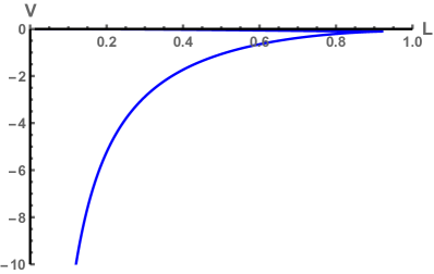
Figure 5: The regularized energy of the bound state in terms of the size of the bound state $L$ in units of $H$. We notice that there is a maximum value of distance $L$ with a maximal energy, beyond which there is no minimal surface with the boundary conditions (39). The turning point occurs for negative values of energy, and the almost flat branch corresponds to the non-stable solutions that are energetically non-favorable.

Notice, however, that the energy of our solution does not cross the horizontal axis. This is different from the behavior in thermal field theory with black hole dual [41, 42]. There the mass subtraction scheme was adopted, and it was found that the energy becomes positive at a certain inter-quarks separation $L_{*}<L_{\rm max}$. This signifies a phase transition where having a pair of straight line strings ending directly on the horizon of the black hole has become the energetically more favorable string configuration. As we do not have a black hole and we have used the Legendre transform scheme for the cancelation of the UV divergences, this explains the absence of such phase transition in our case.

To summarize, we find that similar to the situation of mesons in the usual thermal field theory whose temperature has a holographic origin in terms of a black hole, here our mesons also admit a pair of string solutions for each admissible boundary condition which leads to bound state. However the responsible mechanism here is different: it is due to the presence of cosmological expansion in longitudinal directions parallel to the boundary, rather than attraction due to the black hole in the radial/transverse direction [42, 41]. To elaborate further on the properties of bound state we add one more degree of freedom to our system in the next section.

4 Spinning Mesons in dS Theory

In this section we examine the spinning mesons modeled by rotating hanging strings from the dS boundary.

4.1 The Holographic Setup

The spinning string we consider, has its two endpoints on the boundary, corresponding to the quarks of the spinning meson. To consider rotation, it is convenient to rewrite the planar coordinates metric (38) in the following spherical form

$$ds^{2}=dz^{2}+\sinh^{2}Hz~{}{\left({-dt^{2}+e^{2Ht}{\left({d\rho^{2}+\rho^{2}d\theta^{2}+\rho^{2}\sin^{2}\theta d\phi^{2}}\right)}}\right)}~{}.$$ (59)

Without loss of generality, we consider rotation along the equator of the sphere with the following parametrization ($0\leq\sigma\leq L/2$)

$$t=\tau~{},\qquad\theta=\frac{\pi}{2}~{},\qquad\phi{\left({\sigma,t}\right)}=c+\omega t-\omega f(\sigma)~{},\qquad\rho{\left({\sigma,t}\right)}=\sigma e^{-Ht}~{},\qquad z=z{\left({\sigma}\right)}~{},$$ (60)

where $c$ is a constant to be determined by the two points of the boundary. The function $f{\left({\sigma}\right)}$ parametrize the string world-sheet in the bulk and moreover specifies the initial angle for the spin. The boundary conditions of the string are

$$z{\left({\pm\frac{L}{2}}\right)}=\infty~{},\quad\rho{\left({\pm\frac{L}{2},t}\right)}=\frac{L}{2}e^{-Ht}~{},\quad\phi{\left({\pm\frac{L}{2},t}\right)}=\phi_{\pm}+\omega t~{},\;$$ (61)

where the two endpoints of the string are antipodal in the equator, at $\phi_{+}=0$ and at $\phi_{-}=\pi$. The parametrization (60), (61) describes a string on the equator of the spatial sphere, with antipodal endpoints having an angular velocity $\omega$, and a component of velocity transverse to the spinning motion and along the axis that connects the endpoints, pointing inwards with measure (40), just enough to counterbalance the time dependent expansion of the dS boundary. Below we will solve for the string solution for the region $0\leq\sigma\leq L/2$ subject to the boundary condition (61) at the endpoint $\sigma=L/2$. In addition we will require our solution to satisfy

$$z^{\prime}{\left({\sigma_{0}}\right)}=0~{},\qquad z{\left({\sigma_{0}}\right)}=z_{0}~{},$$ (62)

so that we can extend the solution to the other half $-L/2\leq\sigma\leq 0$. The constant $z_{0}$ is a free parameter that specifies the coordinate of the tuning point of the string.

It turns out that the parametrization (60) is a consistent solution to the full system of equations of motion obtained by the NG action only if the function $f{\left({\sigma}\right)}$ is given by

$$f{\left({\sigma}\right)}=\frac{\log(1-H^{2}\sigma^{2})}{2H}~{}.$$ (63)

Notice that the function (63) happens to be also part of the coordinate transformation from the planar to the static coordinates. Physically, it gives a non-trivial $\sigma$ dependence along the $U(1)$ angle which describes a drag of the string profile in the bulk.

Having specified the function $f{\left({\sigma}\right)}$, we now need to solve the equations of motion to determine $z{\left({\sigma}\right)}$ and obtain the string profile in the bulk. The on-shell action is time independent

$$\frac{4\pi}{\sqrt{\lambda}{\cal T}}S=\int d\sigma\sqrt{\frac{1-\sigma^{2}{\left({H^{2}+\omega^{2}}\right)}}{1-H^{2}\sigma^{2}}\sinh^{2}Hz{\left({\sinh^{2}Hz+{\left({1-H^{2}\sigma^{2}}\right)}z^{\prime 2}}\right)}}:=\int d\sigma\sqrt{D}~{},$$ (64)

and depends explicitly on the worldsheet parameter $\sigma$. Variation of the full action gives only one independent equation of motion and reads

$$z^{\prime\prime}\sinh^{2}Hz{\left({1-H^{2}\sigma^{2}}\right)}{\left({1-{\left({H^{2}+\omega^{2}}\right)}\sigma^{2}}\right)}-z^{\prime 3}{\left({H^{2}+\omega^{2}}\right)}{\left({1-H^{2}\sigma^{2}}\right)}^{2}\sigma$$

$$-\frac{3}{2}z^{\prime 2}\sinh 2Hz{\left({1-H^{2}\sigma^{2}}\right)}{\left({1-{\left({H^{2}+\omega^{2}}\right)}\sigma^{2}}\right)}{}$$

$$-z^{\prime}\sinh^{2}Hz{\left({\omega^{2}+2H^{2}{\left({1-\sigma^{2}{\left({H^{2}+\omega^{2}}\right)}}\right)}}\right)}\sigma{}$$

$$-\sinh^{2}Hz\sinh 2Hz{\left({1-{\left({H^{2}+\omega^{2}}\right)}\sigma^{2}}\right)}=0~{}.$$ (65)

The string carries energy and angular momentum defined by differentiating the Lagrangian with respect to $\dot{t}$ and $\dot{\phi}$ and integrating the densities along the length of the string

$$E_{Q\bar{Q}} = 2\int_{0}^{L/2}d\sigma\;\frac{{\left({1-H^{2}\sigma^{2}}\right)}\sqrt{D}}{1-\sigma^{2}{\left({H^{2}+\omega^{2}}\right)}}~{},$$ (66)

$$J_{Q\bar{Q}} = 2\int_{0}^{L/2}d\sigma\;\frac{-\omega\sigma^{2}}{1-\sigma^{2}(H^{2}+\omega^{2})}\sqrt{D}~{}.$$ (67)

The dependence on the parameter $\omega$ is continuous and by switching it off $\omega=0$, the energy (66) is equal to the static on shell action corresponding to the energy of the bound state of the quark (45), and the angular momentum becomes null. Due to the infinite length of the string both energy and angular momentum are infinite and a regularization is required. The infinite terms that regularize the energy and the angular momentum are given by (50) and applying it to our case we obtain

$$E = E_{Q\bar{Q}}-2\sinh Hz\frac{1-H^{2}\frac{L^{2}}{4}}{\sqrt{1-\frac{L^{2}}{4}(H^{2}+\omega^{2})}}\Bigg{|}_{z\rightarrow\infty}~{},$$ (68)

$$J = J_{Q\bar{Q}}-\frac{-L^{2}\omega\sinh Hz}{2\sqrt{1-\frac{L^{2}}{4}(H^{2}+\omega^{2})}}\Bigg{|}_{z\rightarrow\infty}~{}.$$ (69)

For no rotation, the energy (68) is equal to the one in on shell action corresponding to the energy of the bound state of the quark (55).

4.2 The Spinning String Solutions

The string profile is obtained first by solving the single equation (65) on the region $0\leq\sigma\leq L/2$ and then extend to the other half. That this is possible is based on the following observations: In the region close to the center of the sphere, the string parametrized by (60), (61) does not have a discontinuity along the $\phi$ coordinate, since the minimum point of the string does not rotate. This can be checked by looking at the equations of motion and noticing that in the full action the derivatives $\partial_{\sigma}\phi^{2}$ are multiplied by the term $\sigma^{2}\sinh^{2}Hz(\sigma)$. The function $z(\sigma)$ is even, with a minimum point at $\sigma=0$, so its expansion around $\sigma=0$ is at least of second order. Therefore in the resulting equations of motion the terms involving derivatives of $\phi$ are all zero at $\sigma=0$ and the string solution is smooth there too.

Figure 6: The string world-sheet solution corresponding to a spinning meson($\omega=1$), compared to the static one for fixed bulk distance $z_{0}$. The blue-purple colored outer string solutions are the ones that correspond to the static string, while the inner red-cyan colored strings are the ones corresponding to the spinning state. Notice the spinning strings have less boundary distance between their endpoints, while the deformation of the U-shape string is enhanced due to rotation compared to the static configuration.

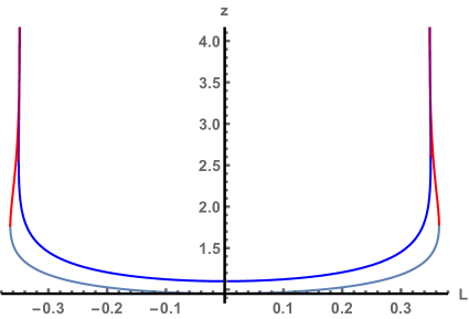
Figure 7: Spinning and static string worldsheets with equal distance string endpoints. The spinning(red-cyan colored) string goes deeper in the bulk and is more deformed compared to the static one. The parameter $\omega$ is chosen equal to the unit.

Our obtained string profiles are presented in the Figures 7 and 7. The deformation of the U-shaped string inside the bulk is enhanced by the spin compared to the static case (Figure 7). Moreover, spinning strings with fixed turning point inter-quark distance $L$ correspond to surfaces that go deeper to the bulk compared to the static strings (Figure 7). This is naturally expected since rotation will tend to increase of the distance between the quarks, while the string tension acts to the opposite direction. This is already a hint that spinning strings dissociate easier than that static ones, however for a rigorous evident we need to compute the energy of the bound states.

In the case of spinning string we have two free parameters that the energy of the state depends on. By fixing the spin of the string and varying the string world-sheet endpoint we can obtain the function $L(z_{0})$. Then we can justify what we have already noticed by comparing spinning and static strings: the first ones correspond to larger inter-quark distances for the same turning point $z_{0}$, compared to the latter ones. This is presented in Figure 9. When we fix the length of the string world-sheet and increase the spin, we obtain a function $\omega(z_{0})$ where notice that the for higher angular velocities the minimal surface goes deeper in the bulk in order to preserve the invariant distance at the boundary (Figure 9). This is in agreement with the previous observations on the string profiles.

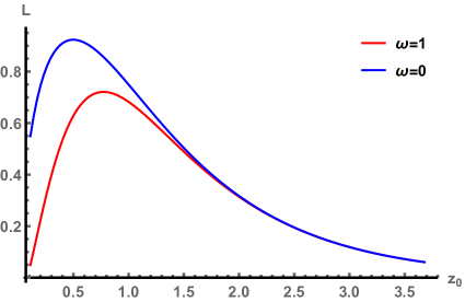
Figure 8: The function $L(z_{0})$ for fixed angular velocity. For each boundary condition, correspond two minimal surfaces. Increase of angular velocity, decreases the maximum length that the state can have.

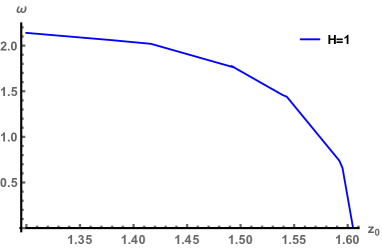
Figure 9: The function $\omega(z_{0})$ for a constant inter-quark distance at the boundary. Decrease of the angular velocity leads to surfaces that go deeper to the bulk in order to preserve the length on the boundary. This explains naturally the finding of the Figure 9.

To observe the dissociation of the quark bound state in relation with spin, we fix the length of the state and the temperature, and modify the angular momentum. To keep a state in constant length as $\omega$ increases, we need a world-sheet that comes closer to the boundary. We find that the angular momentum of the bound state is increasing for increasing $\omega$ until it reaches a maximum value for $\omega=\omega_{\rm max}$, where the decrease begins. For lower temperatures the magnitude of the angular momentum is larger, and the heavy quark bound state can spin faster. This is naturally expected since the string feels less ’friction’ in lower temperatures (Figure 11).

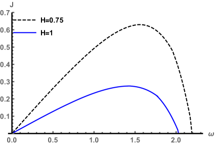
Figure 10: The angular momentum in terms of the angular velocity. There is a maximum spin that the state can reach for a value of $\omega_{\rm max}$. Increase of the temperature allows larger values for the spin and steepest increase.

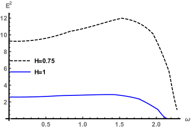
Figure 11: The square of energy versus the angular velocity $E^{2}(\omega)$ for constant inter-quark distance at the boundary. There is an increase of the energy until the angular velocity reaches the value $\omega_{\rm max}$ and after that it decreases. The behavior resembles the angular momentum dependence on $\omega$, presented in Figure 11.

We find that the energy in terms of $\omega$ increases for increasing angular velocity until it reaches a maximum value for $\omega=\omega_{\rm max}$ (Figure 11). Lower temperatures lead to higher energies $E(\omega)$ of the bound state with fixed inter-quark distance. The maximum of the angular momentum and energy occur for the same value of angular velocity. Therefore the expression $E^{2}(J)$ will have a cusp point at $J=J_{\rm max}$ indicating that a state of fixed inter-quark distance can reach to a maximum spin. Moreover, for each value of spin $J<J_{\rm max}$ the state can be found with both energies, the upper and lower segment in the $E^{2}(J)$ function (Figure 12).The upper segment is for large values of $\omega$ and large energies and is not energetically preferable. The lower part of the curve depicts the energy of a stable spinning state, and has a continuous limit to the spin-less state.

The existence of a maximum energy and angular momentum with respect to the angular velocity can be explained by looking at the behavior of the minimal surface. We have shown that for a fixed inter-quark distance and increasing the spin, the surface has to extend deeper to the bulk in order to preserve the invariant distance at the boundary. There is a critical point at which effect of cosmological expansion and rotation becomes so big that it is no longer possible to have a stable bound state.

To summarize our findings in this section, we conclude that the spinning bound state on a dS CFT theory, has all the characteristics of a spinning bound state in a finite temperature dual field theory in flat spacetime. Therefore, it feels the heat bath in a similar way as it would be in gravity dual theory with a black hole, for example as in [44].

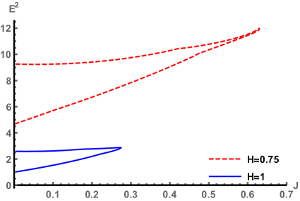
Figure 12: The Energy versus the angular momentum for fixed boundary distance. Notice the maximum reachable spin for the bound state and the fact that for each value of angular momentum the state is allowed to have two energies. The upper segment corresponds to large values of $\omega$ and is unstable and not energetically favorable. Increase of the temperature allow larger values for the spin, and decrease in the energies. The behavior of the bound state is like we have placed it in a finite temperature field theory in flat space.

5 Conclusions and Discussions

In this paper we have examined the thermal properties of the dS field theories in the Bunch-Davies vacuum. We have provided a formalism for the study of the entanglement entropy of a strip in several dimensions. In the special case of $AdS_{3}/dS_{2}$ sliced theory, the logarithmic entanglement entropy is related to the geodesic in the bulk space, and due to conformal invariance the result is expected to agree with the flat space field theories. Nevertheless, we have studied analytically the entropy and by using the geodesic approximation we have found the equal time two point correlator and have reproduced the result obtained using the bulk to boundary formalism in [4].

We have also examined heavy quark probes placed in a strongly coupled de Sitter universe. In the planar coordinates, the spatial part of our metric expands with a rate of $\exp(HT)$. We have considered a pair of a heavy quark and a heavy anti-quark on the dS boundary, where each quark has a constant speed pointing to each other in order to counterbalance the expansion of the spacetime. The heavy meson bound state has a constant invariant inter-quark distance which corresponds to a time-translational invariant world-sheet. We have discussed the numerical implications of the computation due to the presence of cosmological expansion in the bulk and the way to regularize the infinite energy of the pair in holography. The meson bound state share many properties as the bound state in thermal field theories. In particular, it does not exist beyond an inter-quark distance.

By examining the spinning heavy quark bound states our system gets one more degree of freedom. We observe that there is a maximum angular momentum value that the spinning bound state can exist. We compute the energy of the spinning meson, in terms of its angular momentum and conclude that the spinning string realizes the Hawking temperature. It would be very interesting to develop a methodology for other observables in the gravity dual of dS field theories, especially the ones that their evaluation in flat thermal field theories depend heavily on the presence of a black hole horizon, like the jet quenching, and to examine how the generic formulas of [47] would be modified in the present setup. Along these lines we mention the interesting study of fluctuation and dissipation in the de Sitter space [48].

It is worth noting that the effect of the cosmological expansion of the de Sitter factor persists in the bulk and its effect on the string world-sheet is evident. However the effect is different compared to the strings placed in a black hole background where the tidal gravitational attraction of the black hole tends to pull and deforms the string in the radial direction, while the cosmological expansion of the de Sitter factor of the AdS space affects the string in the longitudinal directions parallel to the boundary.

In this paper we have consider de Sitter space written in planar or conformal coordinates. Nevertheless we show that by a suitable choice of ansatz for the string worldsheet, one can eliminate from the effective system all the time dependence consistently. By doing that we end up with time invariant system and ordinary differential equations which are under a good control, instead of the more involved partial differential equations. Therefore, the consideration in this paper may also provide some guidance towards the study of other observables in general time dependent theories.

Appendix A Strings in Static versus Planar Coordinates

Here we provide the coordinate transformation between the planar coordinates of dS space

$$ds^{2}=-dt^{2}+e^{2Ht}(dr^{2}+r^{2}d\Omega)$$ (70)

and the static ones

$$ds^{2}=-(1-H^{2}\tilde{r}^{2})d\tilde{t}^{2}+\frac{1}{1-H^{2}\tilde{r}^{2}}dr^{2}+\tilde{r}^{2}d\Omega~{}.$$ (71)

We find the relation between the coordinate systems by identifying

$$\tilde{r}=e^{Ht}r~{},$$ (72)

which leaves a differential equation to be solved for the time coordinates to get the full transformation

$$\tilde{t}=t-\frac{1}{2H}\log(1-H^{2}r^{2}e^{2Ht})~{},\qquad\tilde{r}=re^{Ht}~{}.$$ (73)

One may use the coordinate transformation to map our string solutions to the static coordinates. By doing that to the static boundary bound state (42) we get on dS

$$\tilde{t}=\tau-\frac{1}{2H}\log(1-H^{2}\sigma)~{},\qquad\tilde{r}=\sigma~{},$$ (74)

while the holographic coordinate is parametrized by another function $z(\sigma)$. We notice that this string solution lead to a different action compared to the solution obtained in [43], but to a similar equation of motion. Moreover, the way we have parametrized the strings in the planar coordinate system does not constrain us to have to use radial coordinates with a finite positive range, and we are allowed to place the string symmetrically, with respect to the origin. We also note that with a coordinate transformation from the planar coordinates to the static ones, one can bring the rotating string solution (60) to a form close to a boosted string in the static coordinates.

References

- [1] N. D. Birrell and P. C. W. Davies, Quantum Fields in Curved Space, Cambridge Univ. Press. (1982) 106008.
-
[2]
See for example,
C. P. Burgess, L. Leblond, R. Holman and S. Shandera,
“Super-Hubble de Sitter Fluctuations and the Dynamical RG,”
JCAP 1003 (2010) 033
doi:10.1088/1475-7516/2010/03/033
[arXiv:0912.1608 [hep-th]].
C. P. Burgess, R. Holman, L. Leblond and S. Shandera, “Breakdown of Semiclassical Methods in de Sitter Space,” JCAP 1010 (2010) 017 doi:10.1088/1475-7516/2010/10/017 [arXiv:1005.3551 [hep-th]]. - [3] A. A. Starobinsky and J. Yokoyama, “Equilibrium state of a selfinteracting scalar field in the De Sitter background,” Phys. Rev. D 50 (1994) 6357 doi:10.1103/PhysRevD.50.6357
- [4] C.-S. Chu and D. Giataganas, AdS/dS CFT Correspondence, arXiv:1604.05452.
- [5] K. Pilch, P. van Nieuwenhuizen, and M. F. Sohnius, de sitter superalgebras and supergravity, Comm. Math. Phys. 98 (1985), no. 1 105–117.
- [6] J. Lukierski and A. Nowicki, All Possible De Sitter Superalgebras and the Presence of Ghosts, Phys. Lett. B151 (1985) 382–386.
- [7] T. Anous, D. Z. Freedman, and A. Maloney, de Sitter Supersymmetry Revisited, JHEP 07 (2014) 119, [arXiv:1403.5038].
- [8] K. Hristov, A. Tomasiello and A. Zaffaroni, “Supersymmetry on Three-dimensional Lorentzian Curved Spaces and Black Hole Holography,” JHEP 1305 (2013) 057 doi:10.1007/JHEP05(2013)057 [arXiv:1302.5228 [hep-th]].
- [9] D. Cassani, C. Klare, D. Martelli, A. Tomasiello and A. Zaffaroni, “Supersymmetry in Lorentzian Curved Spaces and Holography,” Commun. Math. Phys. 327 (2014) 577 doi:10.1007/s00220-014-1983-3 [arXiv:1207.2181 [hep-th]].
- [10] P. de Medeiros and S. Hollands, “Conformal symmetry superalgebras,” Class. Quant. Grav. 30 (2013) 175016 doi:10.1088/0264-9381/30/17/175016 [arXiv:1302.7269 [hep-th]].
- [11] P. de Medeiros and S. Hollands, “Superconformal quantum field theory in curved spacetime,” Class. Quant. Grav. 30 (2013) 175015 doi:10.1088/0264-9381/30/17/175015 [arXiv:1305.0499 [hep-th]].
- [12] D. Cassani and D. Martelli, “Supersymmetry on curved spaces and superconformal anomalies,” JHEP 1310 (2013) 025 doi:10.1007/JHEP10(2013)025 [arXiv:1307.6567 [hep-th]].
- [13] G. Festuccia and N. Seiberg, “Rigid Supersymmetric Theories in Curved Superspace,” JHEP 1106 (2011) 114 doi:10.1007/JHEP06(2011)114 [arXiv:1105.0689 [hep-th]].
- [14] T. T. Dumitrescu, G. Festuccia and N. Seiberg, “Exploring Curved Superspace,” JHEP 1208 (2012) 141 doi:10.1007/JHEP08(2012)141 [arXiv:1205.1115 [hep-th]].
- [15] C. Klare and A. Zaffaroni, “Extended Supersymmetry on Curved Spaces,” JHEP 1310 (2013) 218 doi:10.1007/JHEP10(2013)218 [arXiv:1308.1102 [hep-th]].
- [16] S. Hawking, J. M. Maldacena, and A. Strominger, de Sitter entropy, quantum entanglement and AdS / CFT, JHEP 05 (2001) 001, [hep-th/0002145].
- [17] A. Buchel, Gauge / gravity correspondence in accelerating universe, Phys. Rev. D65 (2002) 125015, [hep-th/0203041].
- [18] A. Buchel, P. Langfelder, and J. Walcher, On time dependent backgrounds in supergravity and string theory, Phys. Rev. D67 (2003) 024011, [hep-th/0207214].
- [19] O. Aharony, M. Fabinger, G. T. Horowitz, and E. Silverstein, Clean time dependent string backgrounds from bubble baths, JHEP 07 (2002) 007, [hep-th/0204158].
- [20] V. Balasubramanian and S. F. Ross, The Dual of nothing, Phys. Rev. D66 (2002) 086002, [hep-th/0205290].
- [21] M. Alishahiha, A. Karch, E. Silverstein, and D. Tong, The dS/dS correspondence, AIP Conf. Proc. 743 (2005) 393–409, [hep-th/0407125]. [,393(2004)].
- [22] S. F. Ross and G. Titchener, Time-dependent spacetimes in AdS/CFT: Bubble and black hole, JHEP 02 (2005) 021, [hep-th/0411128].
- [23] V. Balasubramanian, K. Larjo, and J. Simon, Much ado about nothing, Class. Quant. Grav. 22 (2005) 4149–4170, [hep-th/0502111].
- [24] T. Hirayama, A Holographic dual of CFT with flavor on de Sitter space, JHEP 06 (2006) 013, [hep-th/0602258].
- [25] J. He and M. Rozali, On bubbles of nothing in AdS/CFT, JHEP 09 (2007) 089, [hep-th/0703220].
- [26] J. A. Hutasoit, S. P. Kumar, and J. Rafferty, Real time response on dS(3): The Topological AdS Black Hole and the Bubble, JHEP 04 (2009) 063, [arXiv:0902.1658].
- [27] D. Marolf, M. Rangamani, and M. Van Raamsdonk, Holographic models of de Sitter QFTs, Class. Quant. Grav. 28 (2011) 105015, [arXiv:1007.3996].
- [28] J. Blackman, M. B. McDermott, and M. Van Raamsdonk, Acceleration-Induced Deconfinement Transitions in de Sitter Spacetime, JHEP 08 (2011) 064, [arXiv:1105.0440].
- [29] M. Li and Y. Pang, Holographic de Sitter Universe, JHEP 07 (2011) 053, [arXiv:1105.0038].
- [30] L. Anguelova, P. Suranyi, and L. C. R. Wijewardhana, De Sitter Space in Gauge/Gravity Duality, Nucl. Phys. B899 (2015) 651–676, [arXiv:1412.8422].
- [31] S.-J. Zhang, B. Wang, E. Abdalla, and E. Papantonopoulos, Holographic thermalization in Gauss-Bonnet gravity with de Sitter boundary, Phys. Rev. D91 (2015), no. 10 106010, [arXiv:1412.7073].
- [32] V. Vaganov, Holographic entanglement entropy for massive flavours in dS4, JHEP 03 (2016) 172, [arXiv:1512.07902].
- [33] S. Ryu and T. Takayanagi, Holographic derivation of entanglement entropy from AdS/CFT, Phys. Rev. Lett. 96 (2006) 181602, [hep-th/0603001].
- [34] V. E. Hubeny, M. Rangamani, and T. Takayanagi, A Covariant holographic entanglement entropy proposal, JHEP 07 (2007) 062, [arXiv:0705.0016].
- [35] J. Maldacena and G. L. Pimentel, Entanglement entropy in de Sitter space, JHEP 02 (2013) 038, [arXiv:1210.7244].
- [36] W. Fischler, S. Kundu, and J. F. Pedraza, Entanglement and out-of-equilibrium dynamics in holographic models of de Sitter QFTs, JHEP 07 (2014) 021, [arXiv:1311.5519].
- [37] V. Balasubramanian and S. F. Ross, Holographic particle detection, Phys. Rev. D61 (2000) 044007, [hep-th/9906226].
- [38] T. Banks, M. R. Douglas, G. T. Horowitz, and E. J. Martinec, AdS dynamics from conformal field theory, hep-th/9808016.
- [39] J. M. Maldacena, The large n limit of superconformal field theories and supergravity, Adv. Theor. Math. Phys. 2 (1998) 231–252, [hep-th/9711200].
- [40] E. Witten, Anti-de sitter space and holography, Adv. Theor. Math. Phys. 2 (1998) 253–291, [hep-th/9802150].
- [41] S.-J. Rey, S. Theisen, and J.-T. Yee, Wilson-Polyakov loop at finite temperature in large N gauge theory and anti-de Sitter supergravity, Nucl. Phys. B527 (1998) 171–186, [hep-th/9803135].
- [42] A. Brandhuber, N. Itzhaki, J. Sonnenschein, and S. Yankielowicz, Wilson loops in the large N limit at finite temperature, Phys. Lett. B434 (1998) 36–40, [hep-th/9803137].
- [43] W. Fischler, P. H. Nguyen, J. F. Pedraza, and W. Tangarife, Holographic Schwinger effect in de Sitter space, Phys. Rev. D91 (2015), no. 8 086015, [arXiv:1411.1787].
- [44] K. Peeters, J. Sonnenschein, and M. Zamaklar, Holographic melting and related properties of mesons in a quark gluon plasma, Phys. Rev. D74 (2006) 106008, [hep-th/0606195].
- [45] N. Drukker, D. J. Gross, and H. Ooguri, Wilson loops and minimal surfaces, Phys. Rev. D60 (1999) 125006, [hep-th/9904191].
- [46] C.-S. Chu and D. Giataganas, UV-divergences of Wilson Loops for Gauge/Gravity Duality, JHEP 0812 (2008) 103, [arXiv:0810.5729].
- [47] D. Giataganas, Probing strongly coupled anisotropic plasma, JHEP 1207 (2012) 031, [arXiv:1202.4436].
- [48] W. Fischler, P. H. Nguyen, J. F. Pedraza and W. Tangarife, “Fluctuation and dissipation in de Sitter space,” JHEP 1408 (2014) 028 doi:10.1007/JHEP08(2014)028 [arXiv:1404.0347].