Wadim Kehlkehl@in.tum.de 1
\addauthorTobias Hollholl@in.tum.de 1
\addauthorFederico Tombaritombari@in.tum.de 12
\addauthorSlobodan Ilicslobodan.ilic@siemens.com 13
\addauthorNassir Navabnavab@cs.tum.edu 1
\addinstitution
Computer-Aided Medical Procedures,
TU Munich, Germany
\addinstitution
Computer Vision Lab (DISI),
University of Bologna, Italy
\addinstitution
Siemens AG
Research & Technology Center
Munich, Germany
Octree-based Variational Range Data Fusion
\newfloatcommandcapbtabboxtable[][\FBwidth]
An Octree-Based Approach towards Efficient Variational Range Data Fusion
Abstract
Volume-based reconstruction is usually expensive both in terms of memory consumption and runtime. Especially for sparse geometric structures, volumetric representations produce a huge computational overhead. We present an efficient way to fuse range data via a variational Octree-based minimization approach by taking the actual range data geometry into account. We transform the data into Octree-based truncated signed distance fields and show how the optimization can be conducted on the newly created structures. The main challenge is to uphold speed and a low memory footprint without sacrificing the solutions’ accuracy during optimization. We explain how to dynamically adjust the optimizer’s geometric structure via joining/splitting of Octree nodes and how to define the operators. We evaluate on various datasets and outline the suitability in terms of performance and geometric accuracy.
1 Introduction
3D object reconstruction has been the focus of computer vision for decades and is important for many different fields including manufacturing verification, reverse engineering, rapid prototyping or augmented reality. Recently, the introduction of time-of-flight sensing devices as well as advances in stereo vision and especially the advent of low-cost RGB-D cameras further widened the focus and eased the reconstruction of objects and environments.
Depending on the application the provided range maps are usually either fused into sparse clouds or into volumetric representations. While former are usually faster to store and process, the latter offer the advantage of straight-forwardly defining mathematical operators on the volumes due to the their dense nature. In this paper, we conduct 3D object reconstruction by fusing truncated signed distance fields (TSDF) via a variational optimization approach which would usually require us to store the data in dense volumetric grids. Such a representation entails a high memory consumption and runtime complexity since each discrete voxel has to be stored and also considered during operations. Furthermore, iterative optimization schemes create constantly changing intermediate solutions and thus would require for a dynamic spatial structure that follows the evolving implicit surface by structural updates.
Hierarchical space partitioning schemes, like kD-trees [Bentley(1975)] or Octrees [Meagher(1982)], can tremendously increase query performance for static geometries but need to be properly updated for dynamic changes occurring inside the volume. Obviously, employing partitioning schemes during an optimization must be carefully designed to avoid accumulation of quantization errors which lead to inaccurate solutions. In this work, we build our optimization around Octrees which recursively divide up the space into eight equally-sized cubes according to split and join rules. Octrees are established in many fields and are often used to alleviate computational burdens. Recent work ([Steinbrucker et al.(2013)Steinbrucker, Kerl, Sturm, and Cremers, Chen et al.(2013)Chen, Bautembach, and Izadi, Zeng et al.(2013)Zeng, Zhao, Zheng, and Liu]) uses Octrees for range data integration to map the environment, but employs simple update rules to encompass newly seen data without any optimization whatsoever. For simulation problems these partitioning structures are usually of static auxiliary nature (e.g\bmvaOneDotaccelerating point/surface look-ups, [Calakli and Taubin(2011), Losasso et al.(2004)Losasso, Gibou, and Fedkiw]) and get discarded or recomputed after each iteration.
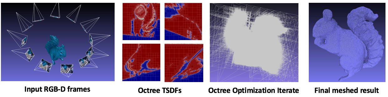
Our novel contribution is to use an Octree as the main optimization structure instead and we present a viable way to robustly fuse TSDFs in a variational approach, similar to [Zach et al.(2007)Zach, Pock, and Bischof, Kehl et al.(2014)Kehl, Navab, and Ilic], while dynamically adapting the Octree’s iterative structure to be faster and memory-efficient. We address the actual creation of the Octrees given initial range maps, the proper definition and calculation of mathematical quantities as well as correct numerical updates that include the iterative reorganization of the solution’s hierarchical partitioning after each step.
2 Related work
In many fields, level-set methods are often employed to solve given problems in e.g. fluid dynamics [Bargteil et al.(2006)Bargteil, Goktekin, O’brien, and Strain, Losasso et al.(2004)Losasso, Gibou, and Fedkiw, Losasso et al.(2006)Losasso, Fedkiw, and Osher], computer graphics [Baerentzen and Christensen(2002), Houston et al.(2006)Houston, Nielsen, Batty, Nilsson, and Museth] or 3D reconstruction [Curless and Levoy(1996), Kolev et al.(2012)Kolev, Brox, and Cremers, Newcombe et al.(2011)Newcombe, Davison, Izadi, Kohli, Hilliges, Shotton, Molyneaux, Hodges, Kim, and Fitzgibbon] where the physical properties of the model act upon the level-set function via PDEs. We refer the reader to a survey on 3D distance fields as a special variant of level-set functions [Jones et al.(2006)Jones, Baerentzen, and Sramek]. In contrast to explicit representations which can entail topological difficulties as well as rendering mathematical operations harder to implement, level-sets can implicitly represent arbitrary shapes and are therefore often preferred. Nonetheless, optimizing in volumetric data always is costly and related work tackled it in the following way:
Similarly to our approach, [Zach et al.(2007)Zach, Pock, and Bischof] also conducts variational data fusion and uses a runlength encoding that allows for fast decompression of the input data but does not address the problem of the structurally-changing minimizer during optimization. In a follow-up work [Zach et al.(2008)Zach, Gallup, Frahm, and Niethammer], the authors propose a coarser quantization of the TSDF values and introduce a point-wise histogram based problem. In [Schroers et al.(2012)Schroers, Zimmer, Valgaerts, Demetz, and Weickert] the authors suggest to modify the data term such that one tries to be similar to the point-wise median. Again, none address the problem of the structurally-changing iterate. The authors of [Popinet(2003)] claim to have the first single-pass hierarchical-based approach for incompressible Euler equations based on multi-grids, although earlier works (e.g. [Strain(1999)]) already focused on tracking moving interfaces with tree-based structures. In [Losasso et al.(2004)Losasso, Gibou, and Fedkiw, Losasso et al.(2006)Losasso, Fedkiw, and Osher], the authors deal with spatially adaptive techniques for incompressible flow and state their surprise about the high accuracy of Octree-based mesh refinement even for small-scale structures. The works [Steinbrucker et al.(2013)Steinbrucker, Kerl, Sturm, and Cremers, Chen et al.(2013)Chen, Bautembach, and Izadi, Zeng et al.(2013)Zeng, Zhao, Zheng, and Liu] use dynamic Octree-based representations to store scene geometry but do no conduct any elaborate schemes for the integration since their main interest is mapping and efficient storage/updates for large-scale problems. [Houston et al.(2006)Houston, Nielsen, Batty, Nilsson, and Museth] introduces a data structure that includes a hierarchical partitioning where each cube uses a runlength encoding. Although very efficient in storage and lookup, online restructuring is rather slow and therefore less suited for iterative structural changes. In [Niessner et al.(2013)Niessner, Zollhöfer, Izadi, and Stamminger] and later [Klingensmith et al.(2015)Klingensmith, Dryanovski, Srinivasa, and Xiao], the authors present an alternative to hierarchical partitioning by hashing the TSDF geometry to enable near-constant time lookups. All of the above mentioned works are focusing only on efficient storage and processing while paying little to no attention to the actual reconstruction quality. We instead are interested in reconstructing objects and thus on how to fuse the range data such that we perform efficiently in terms of memory and runtime while keeping a high reconstruction accuracy.
3 Methodology
Firstly, we show the computation of TSDFs with provided range data and the transformation into their Octree-representations. Secondly, we introduce the new problem formulation and give a way to efficiently solve it via node-wise split/join rules and a fast traversal technique.
Note that in contrast to [Kehl et al.(2014)Kehl, Navab, and Ilic] which fuses into RGB-D volumes, we solely focus here on the geometric minimizer because the space partitioning is not applicable to color volumes. Instead, we compute the coloring after meshing of the 0-isosurface similarly to [Whelan et al.(2013)Whelan, Johannsson, Kaess, Leonard, and McDonald].


3.1 TSDF-Octree generation
The generation of the TSDFs follows related work [Zach et al.(2007)Zach, Pock, and Bischof, Schroers et al.(2012)Schroers, Zimmer, Valgaerts, Demetz, and Weickert, Steinbrucker et al.(2013)Steinbrucker, Kerl, Sturm, and Cremers, Kehl et al.(2014)Kehl, Navab, and Ilic]: given the -th frame of range data together with the corresponding projection , the idea is to compute the signed distance between the surface and each point of the reconstruction volume along the line of sight. Furthermore, scaling with and truncation to is performed to retrieve the final TSDF
| (1) |
where is the projection center for the -th frame in global coordinates. Additionally, we compute for each TSDF a weight volume that signifies whether a voxel has been observed from view or not via a check . Every unseen voxel in front of this hard -threshold is assumed to be solid geometry for a given .
Above scaling factor serves as an uncertainty band and should be well-chosen both to compensate for measurement noise and to clearly divide between outer and interior space (see Figure 3). Strictly speaking, areas which are far apart from the interface consume memory and runtime during optimization without having a drastic influence on the optimizer’s object surface. Our goal is to ensure that these spaces remain computationally inexpensive at all times during the optimization without impairing the final solution. To this end, we transform our problem to work with space-partitioned entities which can adapt to the changing narrow band of our iterated solutions.
Octree construction
We construct TSDF-Octrees from in a top-to-bottom manner. Starting from root node , we define the spread of values subsumed by node in as
| (2) |
with being the subvolume that node represents. Initially, and the spread will be maximal. From here we recursively apply a splitting rule: if the spread at node is higher than a threshold , we subdivide into eight children and proceed further down. This is recursively repeated as long as the condition is fulfilled or until we reach a maximum Octree depth , corresponding to a pre-defined minimum metric voxel size. After the partitioning we propagate the means upwards from the leafs to all inner nodes to speed up computations during later optimization. See Figure 3 for a visual comparison.
3.2 Octree-based variational optimization
Similar to [Zach et al.(2007)Zach, Pock, and Bischof, Schroers et al.(2012)Schroers, Zimmer, Valgaerts, Demetz, and Weickert, Kehl et al.(2014)Kehl, Navab, and Ilic] we fuse all range maps into one volume by finding the minimizer of
| (3) |
where we weight data fidelity against a regularization with a smoothness parameter . [Zach et al.(2007)Zach, Pock, and Bischof] employs an outlier-robust data term together with a Total Variation (TV) regularizer which has the advantage of penalizing the perimeter of the level sets in and in combination, TV- induces a pure geometric regularization, as found in [Chan et al.(2006)Chan, Esedoglu, and Nikolova]. Unfortunately, the non-differentiability requires elaborate solving schemes and we thus follow [Schroers et al.(2012)Schroers, Zimmer, Valgaerts, Demetz, and Weickert, Kehl et al.(2014)Kehl, Navab, and Ilic] by tightly approximating both terms with differentiable quantities
| (4) |
with together with a small being the approximation [Lee et al.(2006)Lee, Lee, Abbeel, and Ng].
An important aspect is the data term normalization since in its current form the functional puts more emphasis on the data term if the number of range images increases. Instead of dividing by the number of images we divide point-wise by the accumulated weight to achieve a spatially consistent smoothing, regardless of how often a voxel has been seen [Schroers et al.(2012)Schroers, Zimmer, Valgaerts, Demetz, and Weickert]. Altogether, this strictly-convex functional can now be solved by gradient descent and in our Octree-based variant, we furthermore replace all quantities with their space-partitioned counterparts to finally retrieve
| (5) |
and instead solve for with a small in the normalizer to avoid division problems for unseen voxels. To optimize Equation 5, we determine the steady state of our PDE
| (6) |
Note that we, strictly speaking, optimize a new in each iteration since we constantly change the structure of our iterate. Nonetheless, this showed to be not a problem in practice since we observed a proper convergence in every case. We will now focus on clarifying how we evaluate above terms and how to conduct the actual optimization in the Octree.

Optimization on the Octree
We conduct the optimization by having at all times only one version of in memory and adjusting the structure while we recursively traverse into each node of . This means that instead of integrating point-wise over the volume, we start from the root and run along the tree while conducting our computations/restructuring on it before proceeding to the next node in the volume in the same pass. To mathematically facilitate the notation, we allow our TSDFs to take nodes as arguments.
For the repartitioning during optimization, we retrieve the gradient descent update at iteration for . Since the update might encompass larger numerical changes, we need to reflect this by restructuring before applying the update such that no crucial information is lost. In contrast to [Losasso et al.(2004)Losasso, Gibou, and Fedkiw, Losasso et al.(2006)Losasso, Fedkiw, and Osher] we do not refine the cube resolution of the Octree simply based on their spatial distance to the narrow band but rather refine them based on numerical values. For an Octree node during our run, we compute, together with a gradient step size , the new value and decide for the repartitioning together with a splitting threshold , a joining threshold and two rules:
-
•
if is a leaf of the Octree and , we split and recurse into the children
-
•
else is not a leaf of the Octree and we check if . If this holds, we recursively conduct the same check for the children and if successful, we join these children only if furthermore they all hold values of equal sign. Otherwise, an implicit surface passes through these nodes and joining them might rupture it.
In order to compute node-wise expressions in our Octree-TSDFs, we simply fetch the corresponding values from the tree nodes that represent the subvolume at this position: if resides at tree level , we either fetch the pre-computed corresponding values and at level , if the level exists, or take the closest leaf that spatially subsumes (see Figure 4). The can be efficiently queried while moving alongside in each Octree.
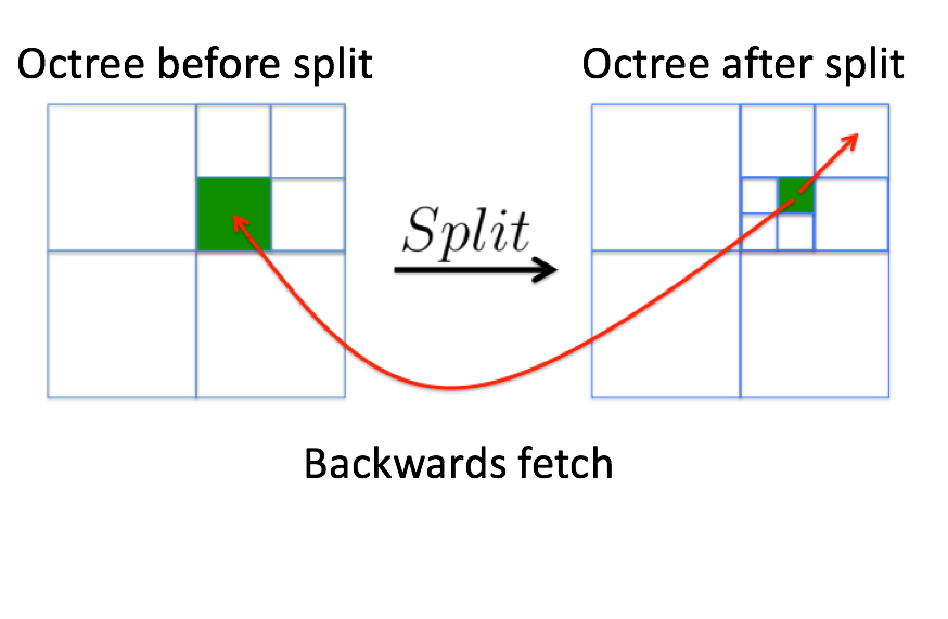
For the more complex quantity, the gradient , we use forward differences which need to be fetched in a neighborhood around each node . This can be easily accomplished during the same pass since we can spatially look-up all nodes ahead of which have not been touched yet. To compute the divergence, we also need to be able to compute backward differences. In our approach we want to be fast and therefore want to accomplish one optimizer iteration in one pass through the Octree. Thus, we immediately restructure all visited nodes and would therefore induce numerical errors if we fetch backwards during the same pass. To remedy that we store for a node its value before splitting such that the computation is proper (see Figure 5). Note that this is not applicable when joining a node since it would need to carry a history of all its children values. However, due to our splitting rules, joins never happen at interfaces and we thus can discard this otherwise problematic issue.
3.3 Meshing and coloring
As a final step, we apply Marching Cubes to extract the 0-level isosurface to retrieve a mesh. To compute the coloring of the resulting mesh, we weigh for each vertex the reprojected colors according to the dot product between its normal and every camera view vector, similar to [Whelan et al.(2013)Whelan, Johannsson, Kaess, Leonard, and McDonald]. Furthermore, to supply color to unseen parts, we iteratively propagate the colors along triangle boundaries and blend the final color in respect to the neighboring, colored vertices and their dot products.
4 Evaluation
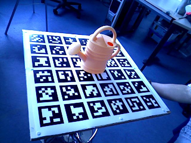
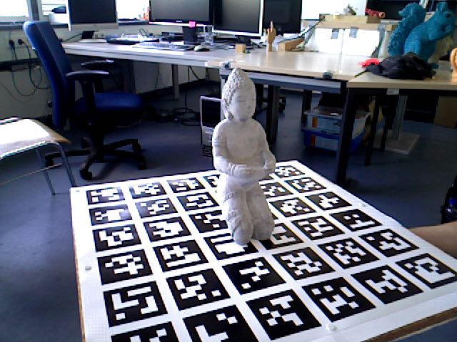
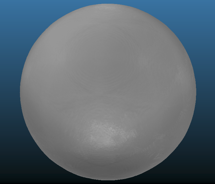
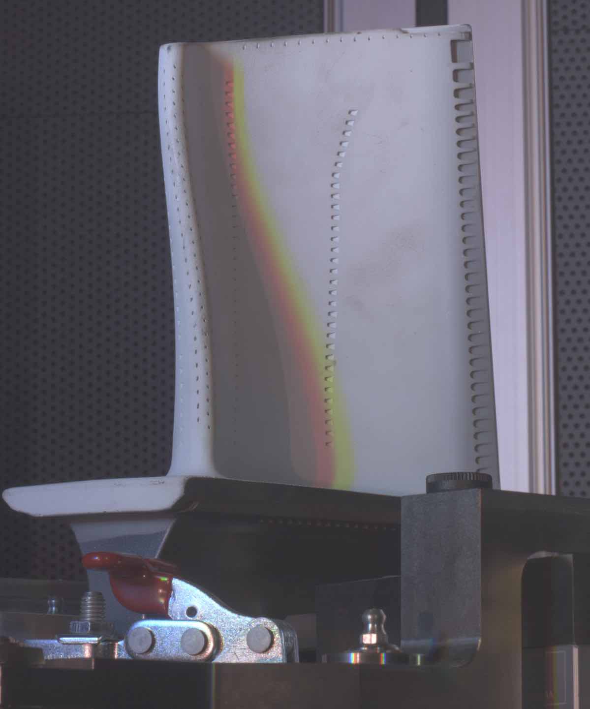
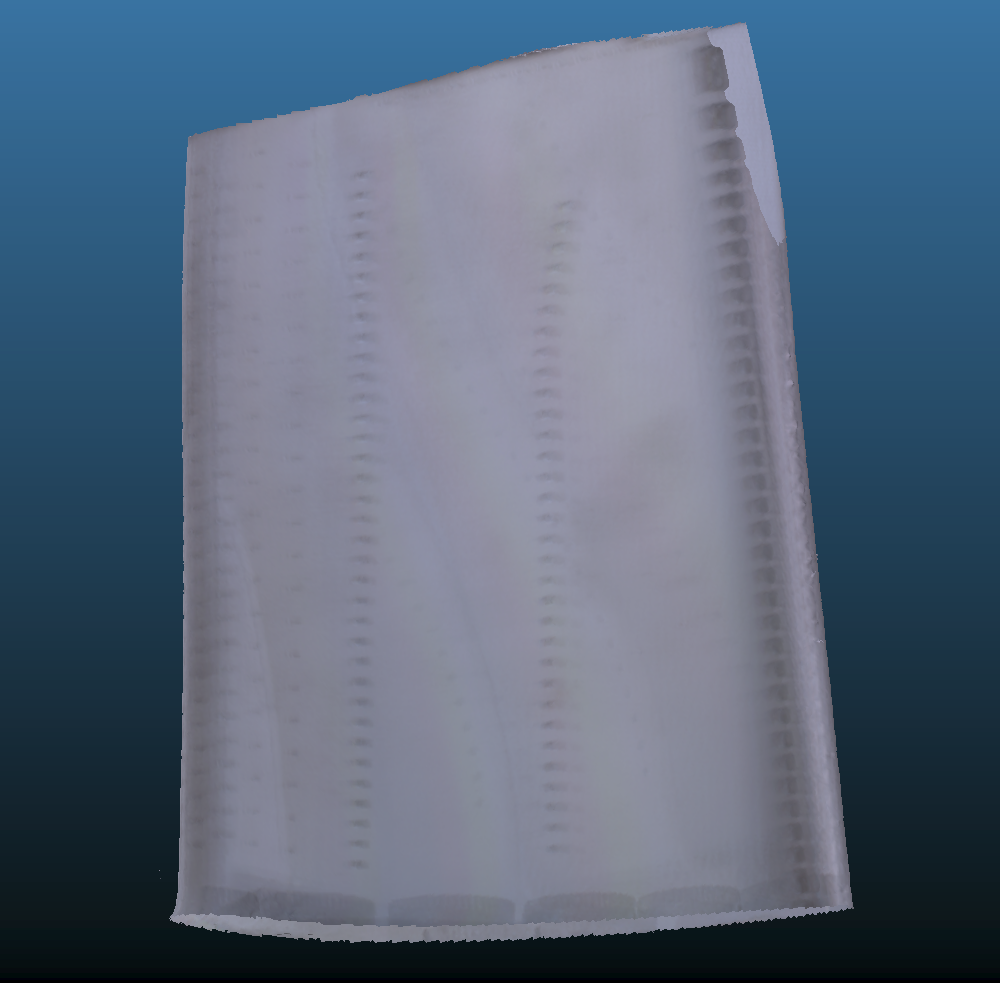
The method was implemented in C++ and the experiments were conducted on a CPU with 32GB of RAM. We ran our experiments on different kinds of data: firstly, we synthetically rendered 31 views of a sphere to measure our loss in accuracy on perfect, noise-free data. Secondly, we acquired sequences of four objects (each consisting of 26 frames) with a commodity RGB-D sensor (Carmine 1.09) to assess the geometrical quality we can achieve with low-cost devices. Lastly, we acquired 24 frames of a turbine blade taken with an industrial high-precision depth sensor (GIS) that provides micrometer precision. Since we have a CAD model of the turbine we evaluate how accurate we can reconstruct real-life objects with state-of-the-art depth sensing technology which is important for manufacturing verification. For comparisons with dense results, we implemented the method from [Kehl et al.(2014)Kehl, Navab, and Ilic].
For the experiments we found that running the optimization for iterations with an initial gradient step size and halving it every iterations was sufficient to converge to good solutions for any object. Furthermore, we fixed but set the metric voxel size and the uncertainty factor depending on the data source. For the synthetic data, we set and , for the Carmine dataset and for the GIS data .


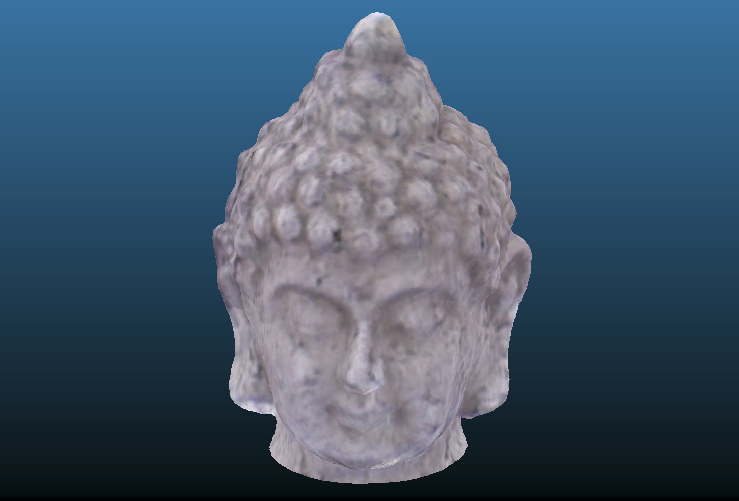
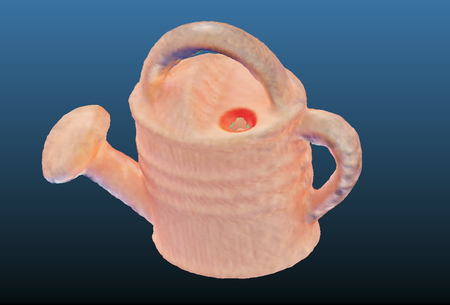
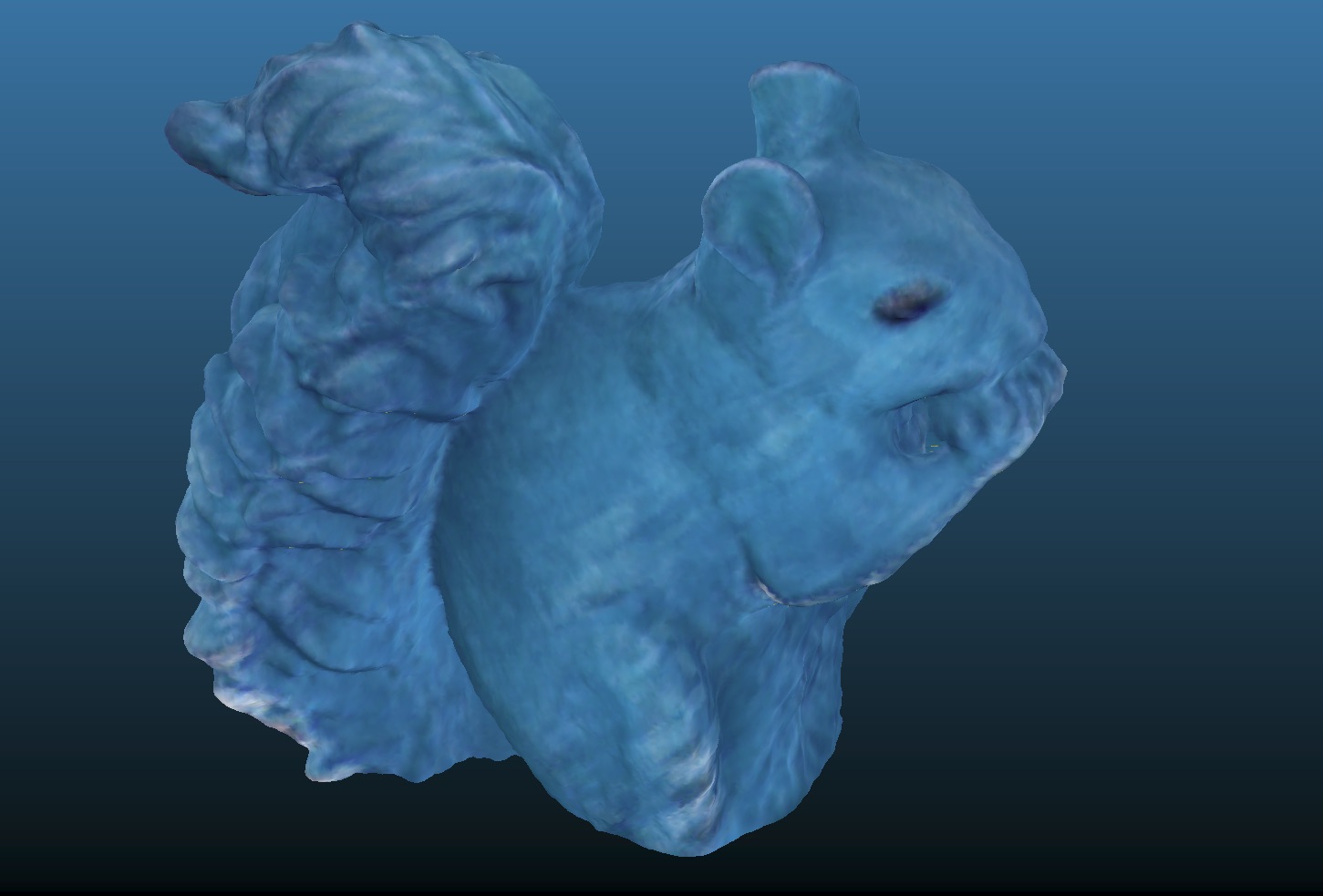


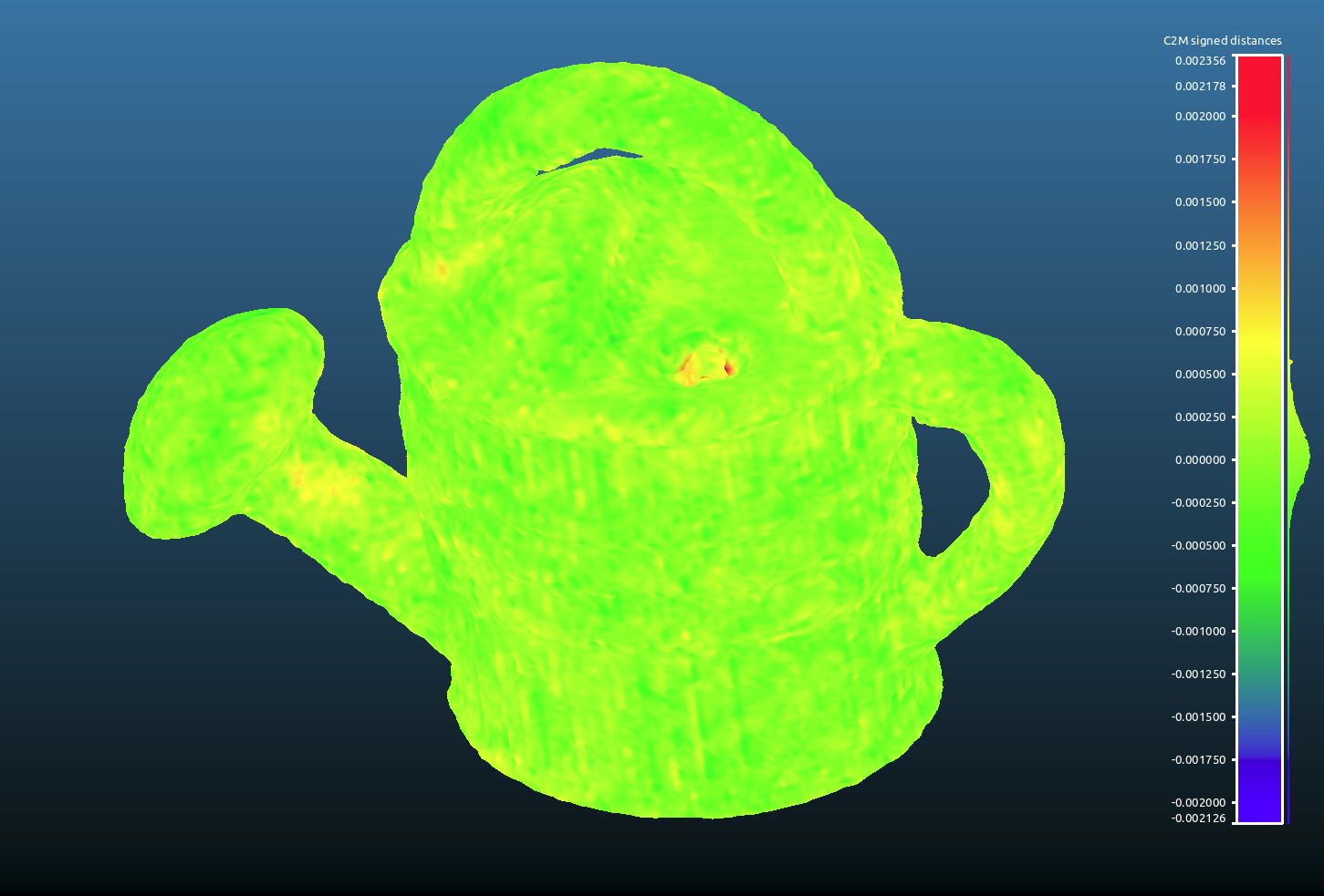
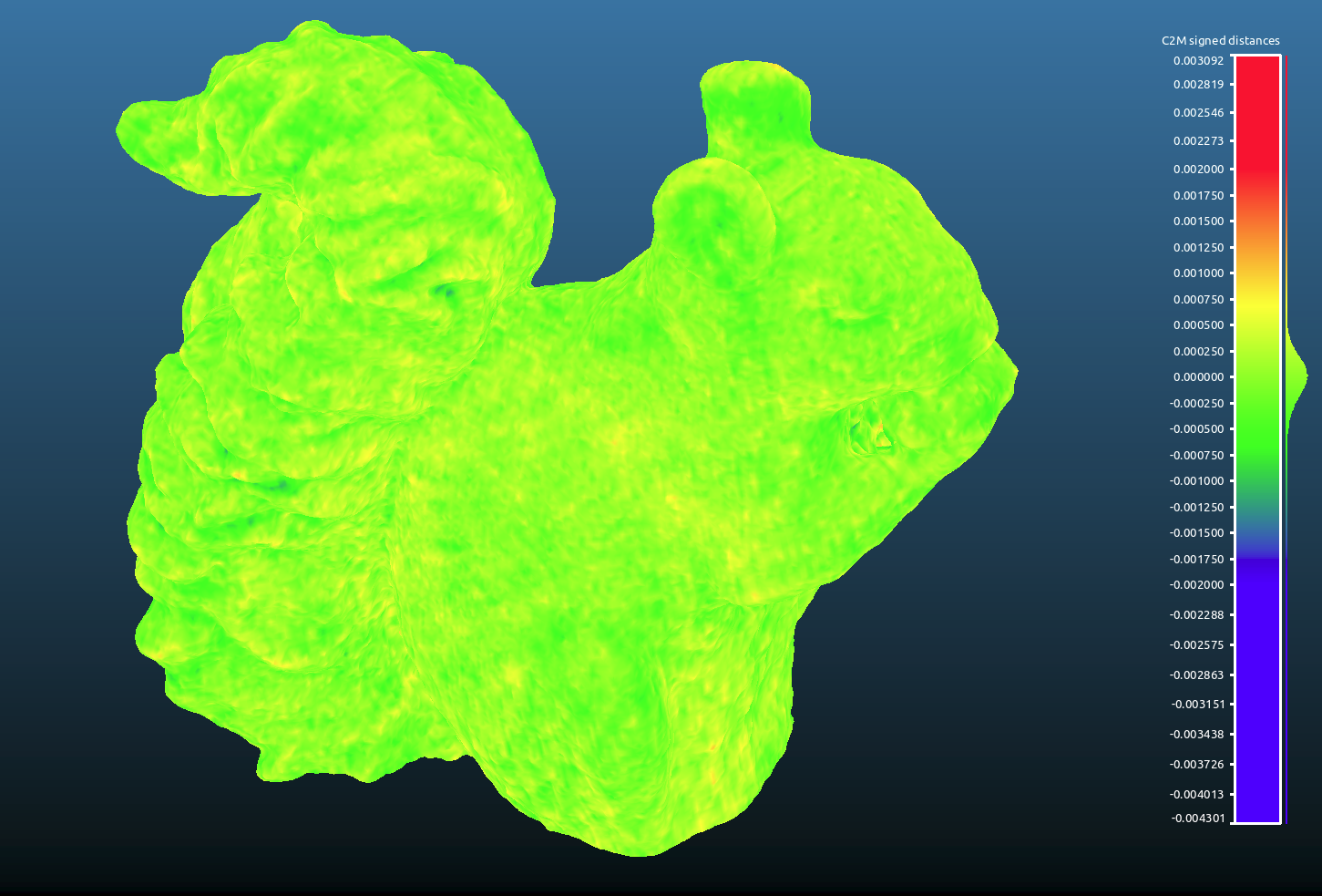
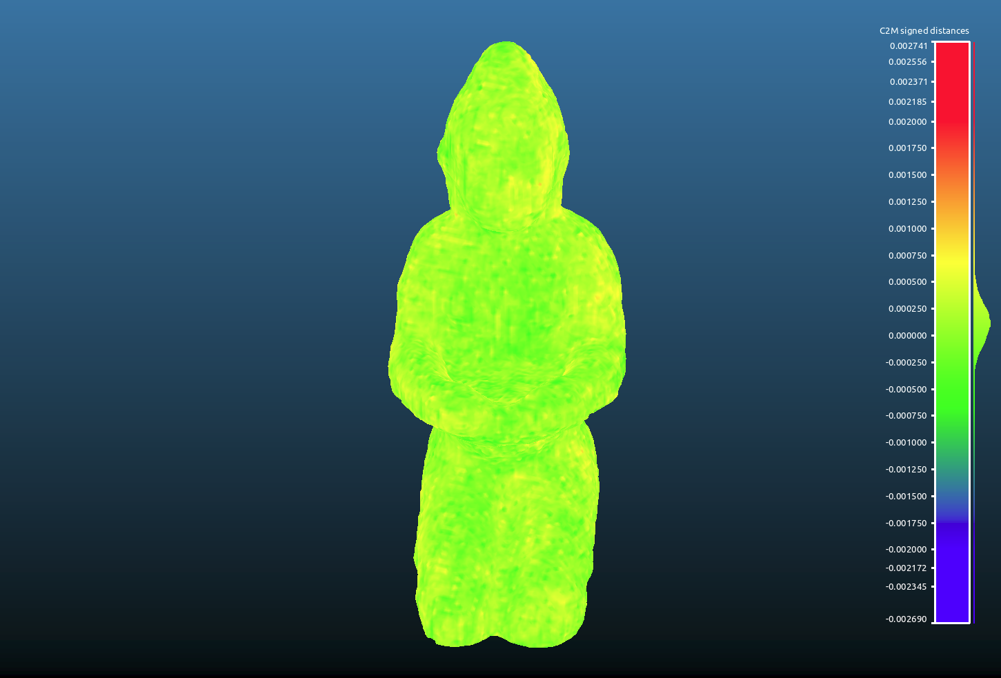
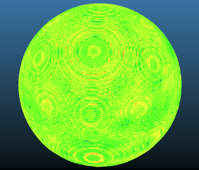
For the Carmine sequences (Figure 6), we constantly retrieve very accurate solutions that are on par with their dense versions. For a more quantitative comparison, we also compare our reconstructions of the ’sphere’ and the ’turbine’ to their groundtruth models (Figures 7 and 8). To compute the vertex-wise difference, we find for each vertex of one reconstruction the closest point of the other reconstruction and compute their distance. The synthetic sphere is nicely reconstructed and the mean error of is virtually negligible. Also the ’turbine’ reconstruction was very accurate with a mean error of which is inside tolerable limits.


4.1 Memory consumption and runtime
Each dense TSDF stores for each voxel the actual distance value and the weight as floats. In comparison, the Octree-TSDF stores per block pointers to 8 children, its parent node and in addition to the above two floats another float value that represents the distance value just before splitting to allow for the computation of the divergence in the same pass. The total amount of memory needed to hold the data term is given in Table 1 and is drastically reduced with the Octree approach for all sequences. To give another interesting insight we plot the memory consumption of during the optimization in Figure 9. While in the dense approach each iterate is constant in memory, its Octree-variant quickly decreases its footprint after more and more blocks get joined. Analogously for the runtime in Table 2, our fast traversing technique allows us to also outperform the dense variants except for the ’squirrel’. While the runtimes for the dense TSDFs are dependent on the volume resolution, the geometry complexity is the main driver of the runtime for the Octree method since frequent repartitionings inbetween iterations can lead to a runtime penalty.


4.2 Split and join
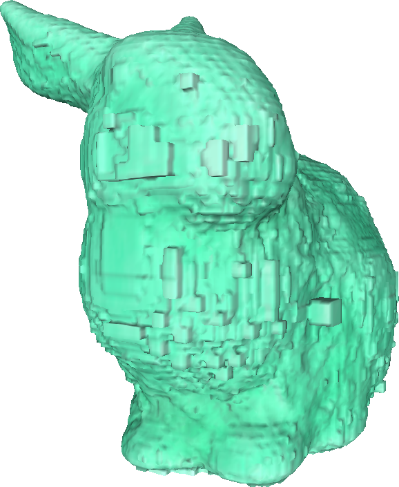
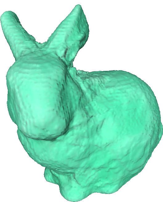
As stated, we apply split and join rules according to thresholds and . Since these values govern the structural density of our Octrees, a careful choice is important to uphold the geometrical accuracy. Splitting early creates a finer partitioning and can lead to unnecessarily high runtime and memory demands while joining too early can result in larger numerical errors since smaller gradient increments get discarded. To have a visual feeling of the impact, we show the fusion of some Carmine frames taken of a 3D print of the Stanford bunny in Figure 11. Apart from the first case that virtually hinders nodes from splitting and leading to massive Octree-artifacts with , the geometry suffers less from quantization with an increasing since it steers how fine the Octree describes the area around the narrow band. Conversely, with a higher we can delay the joining of nodes and thus have the same effect on the area around the band, but from the opposite side, and with a value of actually disabling join operations.
| SDF Size/Res. | Octree Size/Res. | |
|---|---|---|
| sphere | MB / | MB / |
| statue | MB / | MB / |
| head | MB / | MB / |
| squirrel | MB / | MB / |
| can | MB / | MB / |
| turbine | MB / | MB / |
| Dense | Octree | |
|---|---|---|
| sphere | 3.9 | 2.8 |
| statue | 3.7 | 2.6 |
| head | 3.7 | 3.4 |
| squirrel | 3.7 | 4.7 |
| can | 3.7 | 3.2 |
| turbine | 26.1 | 9.5 |
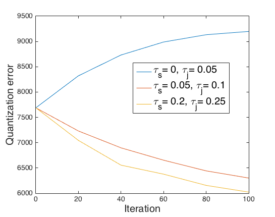

The quantization error between a dense and its induced Octree-version is
| (7) |
and in the ideal case it should be zero for each iterate pair during optimization. As can be seen in Figure 10, the error decreases with higher values of both and whereas in the special case of , the error grows larger due to the lack of splitting, leaving the surface heavily artifacted while the dense version gets smoother.
5 Conclusion
To our knowledge, we are the first to present an approach towards variational range data fusion by partitioning the solutions with a dynamic Octree structure. We have shown how to efficiently conduct restructuring based on iterative node-wise updates of the supplied PDE and that the achieved results are geometrically accurate on multiple datasets and nearly identical to their dense counterparts while being more efficient overall. It would be interesting to investigate further into different ways of computing the required quantities, alternative split/join decisions as well as other solving techniques (e.g. primal-dual [Chambolle and Pock(2011)]).
Acknowledgements
The authors would like to thank Toyota Motor Corporation for supporting and funding this work.
References
- [Baerentzen and Christensen(2002)] Jakob Baerentzen and Niels Christensen. Volume sculpting using the level-set method. In Shape Modeling International, 2002.
- [Bargteil et al.(2006)Bargteil, Goktekin, O’brien, and Strain] Adam W. Bargteil, Tolga G. Goktekin, James F. O’brien, and John a. Strain. A semi-Lagrangian contouring method for fluid simulation. ACM Transactions on Graphics, 25(1):19–38, 2006.
- [Bentley(1975)] Jon Louis Bentley. Multidimensional binary search trees used for associative searching. Communications of the ACM, 18(9):509–517, 1975.
- [Calakli and Taubin(2011)] Fatih Calakli and Gabriel Taubin. SSD: Smooth Signed Distance Surface Reconstruction. Computer Graphics Forum, 30(7), 2011.
- [Chambolle and Pock(2011)] Antonin Chambolle and Thomas Pock. A first-order primal-dual algorithm for convex problems with applications to imaging. Mathematical Imaging and Vision, 40, 2011.
- [Chan et al.(2006)Chan, Esedoglu, and Nikolova] Tony Chan, Selim Esedoglu, and Mila Nikolova. Algorithms for finding global minimizers of image segmentation and denoising models. SIAM Journal on Applied Mathematics, 66:1632–1648, 2006.
- [Chen et al.(2013)Chen, Bautembach, and Izadi] Jiawen Chen, Dennis Bautembach, and Shahram Izadi. Scalable real-time volumetric surface reconstruction. ACM TOG, 32(4):1, 2013.
- [Curless and Levoy(1996)] Brian Curless and Marc Levoy. A volumetric method for building complex models from range images. In SIGGRAPH, 1996.
- [Houston et al.(2006)Houston, Nielsen, Batty, Nilsson, and Museth] Ben Houston, Michael B. Nielsen, Christopher Batty, Ola Nilsson, and Ken Museth. Hierarchical RLE level set: A compact and versatile deformable surface representation. ACM TOG, 25(1), 2006.
- [Jones et al.(2006)Jones, Baerentzen, and Sramek] Mark W. Jones, J. Andreas Baerentzen, and Milos Sramek. 3D distance fields: A survey of techniques and applications. IEEE TVCG, 12(4), 2006.
- [Kehl et al.(2014)Kehl, Navab, and Ilic] Wadim Kehl, Nassir Navab, and Slobodan Ilic. Coloured signed distance fields for full 3D object reconstruction. In BMVC, 2014.
- [Klingensmith et al.(2015)Klingensmith, Dryanovski, Srinivasa, and Xiao] Matthew Klingensmith, Ivan Dryanovski, Siddhartha Srinivasa, and Jizhong Xiao. CHISEL: Real Time Large Scale 3D Reconstruction Onboard a Mobile Device using Spatially-Hashed Signed Distance Fields. In RSS, 2015.
- [Kolev et al.(2012)Kolev, Brox, and Cremers] Kalin Kolev, Thomas Brox, and Daniel Cremers. Fast joint estimation of silhouettes and dense 3D geometry from multiple images. TPAMI, 34(3), 2012. ISSN 01628828.
- [Lee et al.(2006)Lee, Lee, Abbeel, and Ng] Su-In Lee, Honglak Lee, Pieter Abbeel, and Andrew Ng. Efficient L1 Regularized Logistic Regression. In AAAI, 2006.
- [Losasso et al.(2004)Losasso, Gibou, and Fedkiw] Frank Losasso, Frédéric Gibou, and Ron Fedkiw. Simulating water and smoke with an octree data structure. ACM TOG, 23(3), 2004.
- [Losasso et al.(2006)Losasso, Fedkiw, and Osher] Frank Losasso, Ronald Fedkiw, and Stanley Osher. Spatially adaptive techniques for level set methods and incompressible flow. Computers and Fluids, 35(10), 2006.
- [Meagher(1982)] Donald Meagher. Geometric modeling using octree encoding. Computer Graphics and Image Processing, 19(1):85, 1982.
- [Newcombe et al.(2011)Newcombe, Davison, Izadi, Kohli, Hilliges, Shotton, Molyneaux, Hodges, Kim, and Fitzgibbon] Richard A. Newcombe, Andrew J. Davison, Shahram Izadi, Pushmeet Kohli, Otmar Hilliges, Jamie Shotton, David Molyneaux, Steve Hodges, David Kim, and Andrew Fitzgibbon. KinectFusion: Real-time dense surface mapping and tracking. In ISMAR, 2011.
- [Niessner et al.(2013)Niessner, Zollhöfer, Izadi, and Stamminger] Matthias Niessner, Michael Zollhöfer, Shahram Izadi, and Marc Stamminger. Real-time 3D Reconstruction at Scale Using Voxel Hashing. ACM TOG, 32(6), 2013.
- [Popinet(2003)] Stéphane Popinet. Gerris: a tree-based adaptive solver for the incompressible Euler equations in complex geometries. Computational Physics, 190(20), 2003.
- [Schroers et al.(2012)Schroers, Zimmer, Valgaerts, Demetz, and Weickert] Christopher Schroers, Henning Zimmer, Levi Valgaerts, Oliver Demetz, and Joachim Weickert. Anisotropic Range Image Integration. Pattern Recognition, LNCS, 2012.
- [Steinbrucker et al.(2013)Steinbrucker, Kerl, Sturm, and Cremers] Frank Steinbrucker, Christian Kerl, Jürgen Sturm, and Daniel Cremers. Large-scale multi-resolution surface reconstruction from RGB-D sequences. In ICCV, 2013.
- [Strain(1999)] John Strain. Tree Methods for Moving Interfaces. Computational Physics, 151(2), 1999.
- [Whelan et al.(2013)Whelan, Johannsson, Kaess, Leonard, and McDonald] Thomas Whelan, Hordur Johannsson, Michael Kaess, John J. Leonard, and John McDonald. Robust real-time visual odometry for dense RGB-D mapping. In ICRA, 2013.
- [Zach et al.(2007)Zach, Pock, and Bischof] Christopher Zach, Thomas Pock, and Horst Bischof. A globally optimal algorithm for robust TV-L1 range image integration. In ICCV, 2007.
- [Zach et al.(2008)Zach, Gallup, Frahm, and Niethammer] Christopher Zach, David Gallup, Jan Frahm, and Marc Niethammer. Fast Global Labeling for Real-Time Stereo Using Multiple Plane Sweeps. In Proc. of Vision, Modeling and Visualization Workshop, 2008.
- [Zeng et al.(2013)Zeng, Zhao, Zheng, and Liu] Ming Zeng, Fukai Zhao, Jiaxiang Zheng, and Xinguo Liu. Octree-based fusion for realtime 3D reconstruction. Graphical Models, 75(3), 2013.