Two-body physics in the Su-Schrieffer-Heeger model

Abstract

We consider two interacting bosons in a dimerized Su-Schrieffer-Heeger (SSH) lattice. We identify a rich variety of two-body states. In particular, for open boundary conditions and moderate interactions, edge bound states (EBS) are present even for the dimerization that does not sustain single-particle edge states. Moreover, for large values of the interactions, we find a breaking of the standard bulk-boundary correspondence. Based on the mapping of two interacting particles in one dimension onto a single particle in two dimensions, we propose an experimentally realistic coupled optical fibers setup as quantum simulator of the two-body SSH model. This setup is able to highlight the localization properties of the states as well as the presence of a resonant scattering mechanism provided by a bound state that crosses the scattering continuum, revealing the closed-channel population in real time and real space.

I Introduction

In a perfectly periodic system, states outside the allowed bands can appear for both attractive and repulsive interactions when composite objects are formed Hubbard (1963); Mattis (1986). The existence of “exotic” repulsive bound pairs, a.k.a. doublons, has been directly observed for the first time ten years ago by implementing a single-band Hubbard model with ultra-cold Bose gases in an optical lattice Winkler et al. (2006). The study of doublons has been extended to, e.g., long range interacting particles Valiente and Petrosyan (2009); Valiente (2010); Longhi (2012), two-channel models Nygaard et al. (2008); Valiente and Mølmer (2011), superlattices Valiente et al. (2010) and spinor gases Menotti et al. (2016). Aside from presenting behaviours and stability properties interesting by themselves Strohmaier et al. (2010), doublons deeply affect the dynamics of the system. For instance very recently it has been shown that the presence of doublons favours many-body localization in disordered Schreiber et al. (2015) or extended Barbiero et al. (2015) Hubbard models.

On the other hand, any real crystal is made of a bulk and a surface. The study of how surfaces modify the spectrum of a particle in a finite crystal started with the seminal papers by Tamm Tamm (1932) and Shockley Shockley (1939). They pointed out the existence of localized states at the surface with energy outside the allowed energy bands. Such surface states can play an important role in the transport properties. Particular attention has been devoted in the recent years to their characterization in the so-called topological insulator materials Hasan and Kane (2010). The bulk–boundary correspondence provides a link between the presence and number of in-gap edge states and the topological invariants of the bulk crystal. The most famous example is the chiral state on the edge of a two-dimensional integer quantum Hall system (see e.g. Tong ). While most of the above mentioned surface states are well explained by single-particle band theory, the physics becomes much more intriguing in the presence of strong inter-particle interactions.

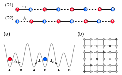
Figure 1: Sketch of the SSH model considered in this work. For OBC and even number of sites, one can obtain two dimerizations: (D1) dimerization $D1$ starting and ending with a strong link $J_{1}$ and (D2) dimerization $D2$ starting and ending with a weak link $J_{2}$. (a) Example of two particles in a dimerized potential described by a Su-Schrieffer-Heeger model; (b) Sketch of the mapping onto a 2D single-particle system: strong links $J_{1}$ (full lines), weak links $J_{2}$ (dashed lines), and local potential $U$ (dark sites).

In this work, we make an important step forward trying to combine a topologically non-trivial single-particle band structure with interactions. A prototypical phenomenon of this kind is the well celebrated fractional quantum Hall effect Tsui et al. (1982); Laughlin (1983). Here, we focus our attention on the minimal model of two interacting particles in a Su-Schrieffer-Heeger (SSH) lattice. The full two-body spectrum can be calculated and very rich physics emerges in spite of the simplicity of the model. In particular we find: (i) hybridization of different channels leading to Fano-Feshbach resonances; (ii) existence of out-of-cell (long range) bound pairs; (iii) edge states for the bound pairs. We conclude by proposing an experimentally realistic optical fiber setup to quantum simulate the two-body SSH model in the laboratory and experimentally highlight our predictions.

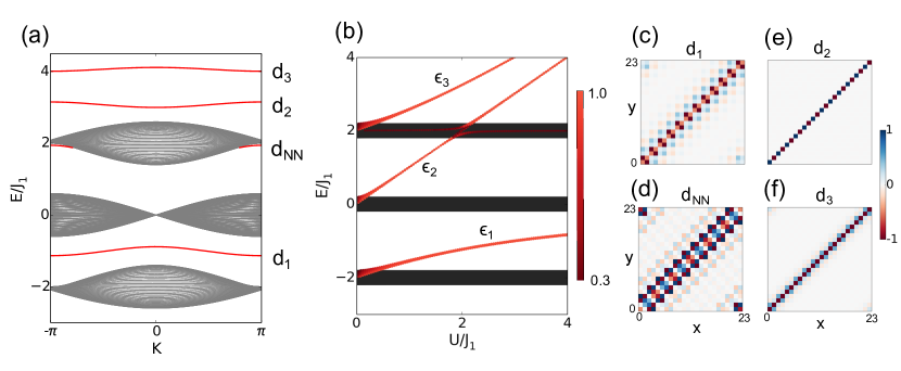
Figure 2: (a) Two-body spectrum for PBC as a function of the center of mass momentum $K$ for $U=3J_{1}$ and $J_{2}=0.3J_{1}$, obtained from scattering theory. The spectrum presents three scattering continua and four bound states $d_{1}$, $d_{NN}$, $d_{2}$ and $d_{3}$. (b) Two-body spectrum as a function of the interaction $U$ for $J_{2}=0.1J_{1}$: The colorscale indicates the sum of onsite and nearest-neighboring site population and highlights the bound states. (c-f) Bound-state wave functions for $U=3J_{1}$ and $J_{2}=0.1J_{1}$ in a chain of $24$ sites at $K=0$ for $d_{1}$(c), $d_{2}$(e), $d_{3}$(f) and at $K=\pi$ for $d_{NN}$(d).

II Model

In this work, we study two interacting bosonic particles in the dimerized lattice shown in Fig. 1 and governed by the Hamiltonian $H=H_{0}+H_{U}$, where

$$H_{0}=-J_{1}\sum_{i}c^{\dagger}_{A,i}c_{B,i}-J_{2}\sum_{i}c^{\dagger}_{A,i+1}c_{B,i}+\mathrm{H.c.}$$ (1)

is the kinetic part providing the single particle SSH model, whereas

$$H_{U}=\frac{U}{2}\sum_{i}\left(c^{\dagger}_{A,i}c^{\dagger}_{A,i}c_{A,i}c_{A,i}+c^{\dagger}_{B,i}c^{\dagger}_{B,i}c_{B,i}c_{B,i}\right)$$ (2)

describes on-site interactions. For later convenience, we define a lattice cell by a pair of $A$ and $B$ sites linked by tunneling $J_{1}>J_{2}>0$, and label each lattice cell with index $i$. For periodic boundary conditions (PBC) the two possible dimerizations are obtained via a shift of a single lattice site, corresponding in practice to the interchange of strong and weak tunneling. For open boundary conditions (OBC) and even number of sites, we define $D1$ the dimerization starting and ending with a strong link $J_{1}$ and $D2$ the dimerization starting and ending with a weak link $J_{2}$ (see Fig. 1(D1,D2)).

In addition to ultra-cold atom implementations, an interesting perspective of our work is to investigate the same physics with 2D lattices of side-coupled optical waveguides, exploiting the mapping of two interacting particles in 1D (Fig. 1(a)) onto a single particle in 2D Longhi (2011); Corrielli et al. (2013). As sketched in Fig. 1(b), the dimerized lattice is reproduced by appropriately-tailored spatially-alternating hoppings in the 2D lattice. Two-body on-site interactions in the 1D system are translated into a local potential $U$ on the diagonal $x=y$ in the single-particle 2D model. A straightforward extension of existing experiments Schreiber et al. (2012); Mukherjee et al. (2015, 2016), would allow the possibility of observing distinctive two-body SSH dynamics directly in real space and real time.

III Bulk system

For periodic boundary conditions (PBC), the single-particle SSH model possesses particle-hole symmetry Ryu and Hatsugai (2002) and the spectrum is formed by two Bloch bands with energy $E_{\pm}(k)=\pm\sqrt{J_{1}^{2}+J_{2}^{2}+2J_{1}J_{2}\cos(k)}$. The two possible dimerizations have the same spectrum, but present a Zak phase difference of $\pi$ Zak (1989); Atala et al. (2013), corresponding to topologically distinct phases identified by different winding numbers Chiu et al. (2016). Apart from the case of hard-core bosons at half-filling (e.g. Grusdt et al. (2013); Deng and Santos (2014)), the interacting Hamiltonian breaks chiral symmetry and a typical two-body spectrum is shown in Fig. 2(a) as a function of the center of mass momentum $K$.

The essential spectrum is not modified by interactions and consists of three scattering continua (type I), obtained by attributing an energy belonging to the single-particle SSH spectrum to each scattering particle. Instead, the wave functions of scattering states are modified by interactions, showing a depletion at zero relative distance by increasing $U$.

In one dimension (1D), any interaction introduces a discrete spectrum, related to the formation of bound pairs. Three bound pairs are readily identified by considering the fully dimerized case $J_{2}=0$. For each cell $i$, the strong-link Hamiltonian admits the three different states (written in the two-body basis $|A_{i}A_{i}\rangle$, $|A_{i}B_{i}\rangle$ and $|B_{i}B_{i}\rangle$)

$$|d_{1,i}\rangle \propto\left(2\sqrt{2}J_{1},U+\sqrt{16J_{1}^{2}+U^{2}},2\sqrt{2}J_{1}\right)\,,$$ (3)

$$|d_{2,i}\rangle \propto(1,0,-1)\,,$$ (4)

$$|d_{3,i}\rangle \propto\left(2\sqrt{2}J_{1},U-\sqrt{16J_{1}^{2}+U^{2}},2\sqrt{2}J_{1}\right)\,,$$ (5)

with energies $\epsilon_{1}=(U-\sqrt{16J_{1}^{2}+U^{2}})/2$, $\epsilon_{2}=U$ and $\epsilon_{3}=(U+\sqrt{16J_{1}^{2}+U^{2}})/2$.

For $J_{2}$ finite, the pairs delocalize along the lattice and develop narrow bands (see Fig. 2). The three bound states $d_{\alpha}$ can be well defined for all values of $K$ at energies either in the band gaps or above the continuum, or cross the continua in some parameter range (see Fig. 2(b)).

Finally, at energies $\sim 2J_{1}$, an additional out-of-cell bound state $d_{NN}$ appears, characterized by a predominant contribution in neighboring cells $(|A_{i}\rangle-|B_{i}\rangle)\otimes(|A_{i+1}\rangle-|B_{i+1}\rangle)$. Such state arises thanks to an effective nearest-neighbor interaction due to virtual processes involving mainly the $d_{2}$ state (see Appendix A.3). The $d_{NN}$ state is present only for momenta around $K=\pi$. This fact can be understood because the emergent nearest-neighbor interaction, which is responsible for the binding, is very weak compared to the bandwidth $2J_{2}$ of the scattering continuum (see for instance Valiente and Petrosyan (2009)). When $\epsilon_{2}=U\sim 2J_{1}$, the $d_{2}$ state becomes resonant with $d_{NN}$ and a strong mixing between the two is observed Fig. 2(d).

III.1 Scattering theory

The spectra of the bound states can be obtained by solving the Lippmann-Schwinger equation on the lattice.

For two particles, it is useful to describe the external degrees of freedom using center-of-mass $R=(x+y)/2$ and the relative coordinates $r=x-y$ for the two particles at lattice positions $x$ and $y$, and the center-of-mass $K=k_{1}+k_{2}$ and relative quasi-momentum $k=(k_{1}-k_{2})/2$. As it usually happens for problems on the lattice, the center-of-mass and relative coordinates do not separate, but still, for PBC, the center of mass momentum $K$ is a good quantum number, allowing to plot the spectrum as $E(K)$. For the sake of clarity, in a dimerized lattice of $N_{c}$ cells of lattice spacing $D$ (corresponding to $N_{s}=2N_{c}$ lattice sites of lattice spacing $d=D/2$) the allowed $K$ values in the first Brillouin zone are given by $K=2\pi\ell/(N_{c}D)$ for $\ell=-N_{c}/2+1,\dots,N_{c}/2$, which, upon Brillouin zone folding, coincide with the allowed $K$ values for a uniform lattice $K=2\pi\ell/(N_{s}d)$ for $\ell=-N_{s}/2+1,\dots,N_{s}/2$.

To develop the scattering theory formalism, it is convenient to write the SSH model in Eq. (1) in a different basis. After performing the canonical transformation

$$p_{i}=\frac{1}{\sqrt{2}}(c_{A,i}+c_{B,i})\,,\qquad m_{i}=\frac{1}{\sqrt{2}}(c_{A,i}-c_{B,i})\,,$$ (6)

the single-particle Hamiltonian is cast into the form

$$H^{\prime}_{0}= -J_{1}\sum_{i}\left(p^{\dagger}_{i}p_{i}-m^{\dagger}_{i}m_{i}\right)$$ (7)

$$-\frac{J_{2}}{2} \sum_{i,\,\nu=\pm 1}\left(p^{\dagger}_{i+\nu}p_{i}-\nu p^{\dagger}_{i+\nu}m_{i}+\nu m^{\dagger}_{i+\nu}p_{i}-m^{\dagger}_{i+\nu}m_{i}\right)\,.$$

Hamiltonian $H^{\prime}_{0}$ describes a particle with pseudo-spin degrees of freedom, labeled as $p,m$, hopping on a one-dimensional lattice. This transformation is useful to treat the two-body problem because the center of mass of each of the two single-particle states $p,m$ is located in the middle of the $A-B$ bond. In a first-quantization description, the two-body wavefunction can be written as

$$|\Psi\rangle=\sum_{x,y,\sigma}\psi^{\sigma}(x,y)|x,y\rangle\otimes|\sigma\rangle\,,$$ (8)

where $x,y$ are, respectively, the unit-cell coordinates of particle 1 and 2, and $|\sigma\rangle\in\mathcal{B}_{\sigma}$ are the two-body spin states

$$\mathcal{B}_{\sigma}=\begin{cases}|+\rangle=|p,p\rangle,\\ |0\rangle=\frac{1}{\sqrt{2}}\left(|p,m\rangle+|m,p\rangle\right),\\ |-\rangle=|m,m\rangle,\\ |F\rangle=\frac{1}{\sqrt{2}}\left(|p,m\rangle-|m,p\rangle\right).\end{cases}\,\vspace*{0.5cm}$$ (9)

For the case of indistinguishable bosons discussed here, the amplitude $\psi^{\sigma}(x,y)$ is symmetric when exchanging $x\leftrightarrow y$, except for the $\sigma=F$ component, which must be antisymmetric in order to provide an overall symmetric wave function. In the pseudo-spin basis, the interaction operator $H_{U}$ is still local, but not diagonal and represented by the matrix

$$H_{U}=\frac{1}{2}\begin{pmatrix}U&0&U&0\\ 0&2U&0&0\\ U&0&U&0\\ 0&0&0&0\end{pmatrix}\,.$$ (10)

In the center-of-mass and relative coordinates, we make the standard ansatz $\psi^{\sigma}(x,y)\equiv e^{iKR}\psi^{\sigma}(r)$ where $K=k_{1}+k_{2}$ is the center-of-mass momentum. This choice of coordinates and the choice of basis $\mathcal{B}_{\sigma}$ allow to decouple the center of mass from the relative motion. After straightforward but tedious calculations, we obtain the Schrödinger equation

$$\left[H^{2B}_{0}+\delta_{r,0}H_{U}\right]_{\sigma,\sigma^{\prime}}\psi^{\sigma^{\prime}}(r)=E\,\psi^{\sigma}(r)\,,$$ (11)

where the kinetic part of the two-body Hamiltonian reads

$$H^{\textrm{2B}}_{0}=\begin{pmatrix}-2J_{1}-J_{2}\cos(K/2)\Delta^{+}_{r}&-i\frac{J_{2}}{\sqrt{2}}\sin(K/2)\Delta^{+}_{r}&0&\frac{J_{2}}{\sqrt{2}}\cos(K/2)\Delta^{-}_{r}\\ i\frac{J_{2}}{\sqrt{2}}\sin(K/2)\Delta^{+}_{r}&0&-i\frac{J_{2}}{\sqrt{2}}\sin(K/2)\Delta^{+}_{r}&-iJ_{2}\sin(K/2)\Delta^{-}_{r}\\ 0&i\frac{J_{2}}{\sqrt{2}}\sin(K/2)\Delta^{+}_{r}&2J_{1}+J_{2}\cos(K/2)\Delta^{+}_{r}&\frac{J_{2}}{\sqrt{2}}\cos(K/2)\Delta^{-}_{r}\\ -\frac{J_{2}}{\sqrt{2}}\cos(K/2)\Delta^{-}_{r}&-iJ_{2}\sin(K/2)\Delta^{-}_{r}&-\frac{J_{2}}{\sqrt{2}}\cos(K/2)\Delta^{-}_{r}&0\end{pmatrix}\,.$$ (12)

Here, we defined the discrete operators $\Delta^{+}_{r}\psi^{\sigma}(r)=\psi^{\sigma}(r+1)+\psi^{\sigma}(r-1)$ and $\Delta^{-}_{r}\psi^{\sigma}(r)=\psi^{\sigma}(r+1)-\psi^{\sigma}(r-1)$.

The Lippmann-Schwinger equation for the bound states reads

$$\psi^{\sigma}(r) =\langle r\sigma|\hat{G}(E)\hat{H}_{U}|\psi\rangle$$

$$=\sum_{\sigma^{\prime},\,\sigma^{\prime\prime}}\int\frac{dk}{2\pi}e^{ikr}G^{\sigma\sigma^{\prime}}(k,E)(H_{U})_{\sigma^{\prime}\sigma^{\prime\prime}}\psi^{\sigma^{\prime\prime}}(0)$$

$$=\sum_{\sigma^{\prime},\,\sigma^{\prime\prime}}G^{\sigma\sigma^{\prime}}(r,E)(H_{U})_{\sigma^{\prime}\sigma^{\prime\prime}}\psi^{\sigma^{\prime\prime}}(0)\,,$$ (13)

where we have defined

$$\hat{G}(k,E)=(E-H^{2B}_{0}(K,k))^{-1}\,.$$ (14)

This formalism has been used to calculate the bound state spectrum shown in Fig. 2(a).

III.2 Resonant scattering

The first noteworthy bulk feature of the two-body SSH model, persisting for any boundary condition, is the strong mixing of the $d_{2}$ bound-state narrow band and type I scattering continuum around the resonance condition $U=2J_{1}$, where the bound-state energy $U$ matches the energy of a scattering state. This mixing leads to a Fano-Feshbach resonance in a lattice Nygaard et al. (2008); Valiente and Petrosyan (2009), and can be described analytically by using a two-channel scattering theory, as shown below. The occurrence of scattering resonances due to repulsive bound states in multi-band Hamiltonians has been studied also in other contexts Valiente and Mølmer (2011); Menotti et al. (2016).

A Feshbach-like resonant scattering process is numerically illustrated in Fig. 3, where we plot the square modulus of the two-body wave function $\psi(x,y)$ at times before, during and after the collision. At $t=0$ we prepare two single-particle gaussian wave packets at momenta $k_{1}=k$ and $k_{2}=-k$ in the upper band of the SSH model, localized at symmetric positions with respect to the lattice center, sufficiently far from the boundaries and from each other, as shown in Fig. 3(a). This initial state belongs to the two-body scattering continuum centered around energy $2J_{1}$. The time evolution in the presence of interactions $U$ is calculated numerically. After collision, we observe two scattered wavepackets and a sizable population of a two-body bound wavepacket of type $d_{2}$, highly localized along $x=y$. At the beginning, the population of the bound state is localized at the center of the lattice, then it expands at a very slow rate along the $x=y$ direction while it decays in scattering states.

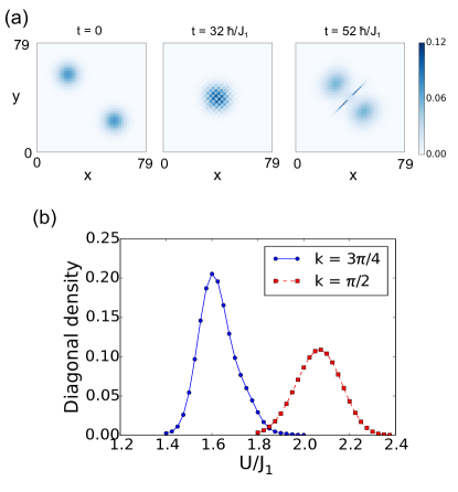
Figure 3: (a) Modulus of the two-body wavefunction $|\psi(x,y)|$ for two incident wave packets before, during and after collision for $J_{2}=0.1J_{1}$, $U=2J_{1}$, $k=\pi/2$ and $L=80$ sites; time is measured in units of $\hbar/J_{1}$; (b) Diagonal density $\sum_{x}|\psi(x,x)|^{2}$ after collision as a function of $U$ for two different $k$ and incident energies $E_{k=3\pi/4}=1.65J_{1}$ and $E_{k=\pi/2}=2.08J_{1}$.

In Fig. 3(b), we plot the diagonal density $\sum_{x}|\psi(x,x)|^{2}$ providing a measure of the occupation of the bound state at a time sufficiently after collision ($t=68\,\hbar/J_{1}$) for two different values of the incident relative momenta, namely $k=3\pi/4$ and $k=\pi/2$, as a function of interaction $U$. As expected, a clear resonance peak is visible at $U$ such that the energy of the bound state matches the energy of the incident wave packets. The different heights of the two peaks can be understood as a consequence of the finite life-time of the bound state and from the fact that the wave packets are moving with different group velocities.

To obtain further understanding of these results, one can perform a crude approximation and develop a theory including only states $|0\rangle$ and $|-\rangle$. Indeed, $|0\rangle\equiv(|p,m\rangle+|m,p\rangle)/\sqrt{2}=|A,A\rangle-|B,B\rangle$ is the dominant pseudo-spin component for $d_{2}$ when $J_{2}\ll J_{1},U$. Analogously, the pseudo-spin state $|-\rangle=(|A\rangle-|B\rangle)\otimes(|A\rangle-|B\rangle)/2$ describes the scattering states at energy $\sim 2J_{1}$.

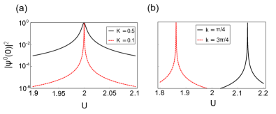
Figure 4: Population $|\Psi^{0}(0)|^{2}$ in the $|0\rangle$ component at $r=0$ as a function of $U$ for: (a) center of mass momentum $K=0.5$ and $0.1$ at fixed $k=\pi/2$ and (b) relative momentum $k=\pi/2$ and $3\pi/4$ at fixed $K=0.3$. In all cases, the center of the resonance coincides with the energy $E$ of the scattering particles.

The coupling of the other states $|+\rangle$ and $|F\rangle$ should be introduced perturbatively in $J_{2}$. However, since Hamiltonian (12) already contains a coupling between $|0\rangle$ and $|-\rangle$, the physics is captured in a qualitative manner even neglecting all other states. The reduced theory therefore reads

$$\tilde{H}_{0}^{\textrm{eff}}(k)=\begin{pmatrix}0&-iJ_{2}\sqrt{2}\sin\left(\frac{K}{2}\right)\cos k\\ iJ_{2}\sqrt{2}\sin\left(\frac{K}{2}\right)\cos k&2J_{1}+2J_{2}\cos\left(\frac{K}{2}\right)\cos k\end{pmatrix}$$

and

$$\tilde{H}_{U}=\begin{pmatrix}U&0\\ 0&U/2\end{pmatrix}.$$ (15)

The Green’s function can be readily calculated and one finds

$$G_{11}(r) = \frac{\delta_{r,0}}{E},$$ (16)

$$G_{22}(r) = i\frac{e^{ikr}}{J_{2}\cos(K/2)\sin k},$$

$$G_{12}(r) = e^{ikr}\frac{1}{\sqrt{2}E}\frac{\tan(K/2)}{\tan k}+\delta_{r,0}\frac{i}{\sqrt{2}E}\tan(K/2),$$

where $E=2J_{1}+2J_{2}\cos(K/2)\cos k$ is the non-interacting spectrum obtained neglecting the off-diagonal terms in $\tilde{H}_{0}^{\textrm{eff}}$. The most general solution of the Schrödinger equation is given by the two-component spinor $\Psi(r)=(\Psi^{0}(r),\Psi^{-}(r))^{T}$:

$$\Psi(r)=\Phi(r)+G(r)\tilde{H}_{U}(1-G(0)\tilde{H}_{U})^{-1}\Phi(0)\,,$$ (17)

where $\Phi(r)$ is solution of the non-interacting problem. To compare with the numerical results presented above, we take the ansatz $\Phi(r)=e^{ikr}(0,1)^{T}$. According to this ansatz, $\Phi(r)$ populates only the $|-\rangle$ component and the two particles have relative momentum $k$, thus modeling two incident particles belonging to type I continuum scattering off each other.

The population of bound state $d_{2}$ is described by the $|0\rangle$ component of $\Psi(r)$ at $r=0$ (on-site pairs), namely $\Psi^{0}(0)$. The results are shown in Fig. 4. A sharp resonance occurs at $U\sim E$, analogous to the one observed in the numerical simulation of the dynamics of two colliding wave packets. When the energy of the incident particles is close to $U$, which is approximately the energy of the bound state, the probability to form the bound state becomes maximal. Note how the resonance becomes sharper when the center of mass momentum $K\rightarrow 0$. Indeed, for $K=0$ the off-diagonal terms in $\tilde{H}_{0}^{\textrm{eff}}$ vanish, thus decoupling the two channels $|0\rangle$ and $|-\rangle$.

IV Edge physics

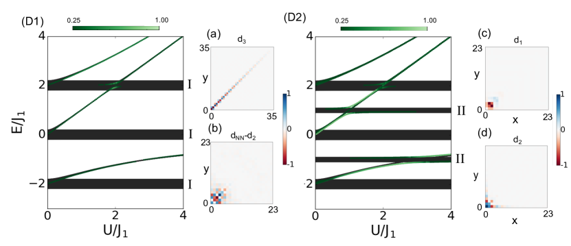
Figure 5: Spectrum with OBC for $J_{2}=0.1J_{1}$ as a function of $U$ for (D1) dimerization $D1$ and for (D2) dimerization $D2$; The green colorscale represents the density in the first and last $2$ lattice cells and highlights the localization of EBS states; (a) $D1/d_{3}$ EBS for $U=3J_{1}$ and energy $E\sim 4J_{1}$, (b) $D1/d_{NN}-d_{2}$ EBS for $U=2J_{1}$ and energy $E\sim 1.9J_{1}$, (c) $D2/d_{1}$ EBS for $U=2J_{1}$ and energy $E\sim-1.3J_{1}$ and (d) $D2/d_{2}$ EBS for $U=J_{1}$ and energy $E\sim 0.8J_{1}$ obtained by exact diagonalization of $72$ lattice sites.

We now discuss the case of open boundary conditions (OBC) to address the effect of interactions on the finite chain SSH model. As usual, we need to distinguish the two possible dimerizations $D1$ and $D2$. Single-particle edge states, typical of dimerization $D2$, combined with a freely propagating particle generate two further continua around energies $\pm J_{1}$ (type II). Obviously, such type II continua are absent in $D1$, which does not admit single-particle edge states (see Fig. 5(D1,D2)). The two (type I and type II) continua and the narrow bands of bound states are independent consequences of the single-particle SSH model and of two-body interactions, respectively. Instead, as a pure consequence of the interplay between SSH geometry, interactions and boundary conditions, intriguing two-body edge bound states (EBS) emerge in the spectrum (see Fig. 5(a-d)). Their presence or absence is highly non-trivial and essentially driven by a renormalization of the edge properties (see also Refs. Pinto et al. (2009); Bello et al. (2016)) .

Such EBS can be associated to the different bound states $d_{i}$. For PBC the associated bound states - when well defined in the whole Brillouin zone - present a two-particle generalized Zak phase difference of $\pi$ for the two dimerizations $D1$ and $D2$. However, as we are going to show in the following, this does not necessarily correspond to the formation of EBS in the finite chain, leading to a breaking of the standard bulk-boundary correspondence. Furthermore, most remarkably, as clearly visible in Fig. 5(D1,D2), EBS appear not only in dimerization $D2$ but also in dimerization $D1$, which does not admit edge states in the single-particle case.

The $D1/d_{3}$ and $D2/d_{1,2}$ EBS can be interpreted as Tamm states of an effective strong-dimerization theory, as it will be detailed below. Localization persists even when the EBS energy enters the scattering continua for $U\rightarrow 0$ Hsu et al. (2016); Della Valle and Longhi (2014). Moreover, immersed in the higher type I scattering continuum, we find a further EBS, which is present in both dimerizations and can be related to the existence of the out-of-cell bound state $d_{NN}$. Hybridization between $d_{NN}$ and $d_{2}$ around $U\sim 2J_{1}$ induces a very strong localization at the edges of a wavefunction with strong both diagonal and out-of-cell characters (see Fig. 5(b)).

IV.1 Strong-dimerization limit

In order to understand the physics behind bound states and EBS, it is useful to consider the regime of strong dimerization $J_{2}\ll J_{1},U$. Here, effective models accounting for the weak tunneling $J_{2}$ in second order perturbation theory can be developed. The building blocks for the effective theory are naturally the three strong-link two-body eigenstates given in Eqs. (3-5). The effective lattice is provided by the lattice cells $i$. More details can be found in Appendix A.

In-cell dimers $d_{\alpha,i}$ can tunnel at second order through intermediate states given by a particle in link $i$ and a particle in a neighboring link $j$. The effective model reads

$$H_{\textrm{eff}}=\sum_{i,\alpha}E_{\alpha,i}\,d^{\dagger}_{\alpha,i}d_{\alpha,i}+\sum_{\langle i,j\rangle}\sum_{\alpha,\beta}J_{\alpha\beta}^{ij}\,d^{\dagger}_{\alpha,i}d_{\beta,j}\,.$$ (18)

The parameters that appear in the model above are second order in the weak tunneling $J_{2}$. The effective model in Eq. (18) provides an accurate prediction of the bound state spectrum away from $U\sim J_{1}$ and $U\sim 2J_{1}$ where bound state $d_{2}$ crosses type II and type I scattering continua, respectively, or $U\sim 3J_{1}$ where $d_{1}$ crosses the lower type II continuum. Relying on the additional assumption that the bound states are well separated in energy and the coupling among them is weak, effective model (18) can be further simplified through a single band approximation, which only keeps $J_{\alpha\alpha}^{ij}$ and $E_{\alpha,i}$ for each state $d_{\alpha,i}$.

Just below the $d_{3}$ bound-state narrow band in dimerization $D1$, one finds EBS $D1/d_{3}$ (see Fig. 5(a)), which can be quantitatively explained as a Tamm state in the framework of effective model (18). The comparison between the results obtained with exact diagonalization and with the effective model is shown in Fig. 6. The localization length of EBS $D1/d_{3}$ is very large. It increases for strong interactions $U\gg J_{1},J_{2}$, so that, for practical purposes, in a finite lattice this state undergoes a crossover to a not exponentially-localized state.

A deeper understanding of the physics underlying the divergence of the localization length for large interactions can be obtained via a much simpler strong-interaction effective model. The states $d_{2}$ and $d_{3}$ are almost degenerate for $U\gg J_{1},J_{2}$. In this limit, a more convenient basis is given by on-site doublons $d^{\dagger}_{A,i}|0\rangle\equiv|A_{i}A_{i}\rangle$ and $d^{\dagger}_{B,i}|0\rangle\equiv|B_{i}B_{i}\rangle$ coupled among each other via second order processes. The corresponding effective Hamiltonian is nothing else than an effective single-particle SSH model with effective hopping coefficients $J_{1,2}^{\textrm{eff}}=-2J_{1,2}^{2}/U$ and effective on-site energy $\epsilon_{\textrm{bulk}}=U+2(J_{1}^{2}+J_{2}^{2})/U$. Moreover, for dimerization $D\sigma$ (with $\sigma=1,2$), the on-site energy of a doublon at the edge results $\epsilon_{\textrm{edge}}=\epsilon_{\textrm{bulk}}+\Delta E_{\sigma}$, with $\Delta E_{\sigma}=-2J_{3-\sigma}^{2}/U$. This energy shift at the outermost sites provides a generalization of the Tamm physics to the SSH model, which in general, depending on $\Delta E$, allows both for Tamm-like states above or below the continua and in-gap states. However, the specific case of our effective model coincides, in both dimerizations, exactly with the critical value of $\Delta E$ for which neither Tamm nor in-gap states can exist (see discussion in Appendix A.2). This implies that in the strong-interaction limit $U\gg J_{1}$ exponentially localized edge states are not to be expected in finite-size chains, in agreement with the numerical results.

For dimerization $D2$, a closer inspection of the $d_{1}$ and $d_{2}$ dimer spectra around their intersection with type II continua shows a peculiar feature: two dimer states, gapped from their continua, appear (see Fig. 5(c-d)). They correspond to pairs of $D2/d_{1,2}$ EBS moved out of the corresponding bound-state narrow bands as a consequence of the renormalized parameters at the boundaries.

These EBS can also be accounted for by effective model (18). In $D2$, the effective model is slightly more complicated than in $D1$, since no full lattice cell is present at the edges, but rather a single lattice site (see Fig. 1(D2)). In the following, we thus specialize to the case of the $D2/d_{2}$ state. While in the bulk the bound state preserves its standard form $|d_{2,i}\rangle=(|A_{i},A_{i}\rangle-|B_{i},B_{i}\rangle)/\sqrt{2}$, for the doublons at the edges one needs to consider the ansatz $|d_{2,0}\rangle=-|B_{0},B_{0}\rangle$ and $|d_{2,L}\rangle=|A_{L},A_{L}\rangle$. This truncated bound-state wave function affects both the effective hopping $J_{22}^{\textrm{edge,D2}}\neq J_{22}^{\textrm{bulk}}$, the on-site energy $E_{2}^{\textrm{edge,D2}}\neq E_{2}^{\textrm{bulk}}$ at the edges, and the on-site energies $E_{2,1},E_{2,L-1}$ at the outermost complete lattice cells. As shown in Fig. 7 (blue lines), sufficiently far away from the $U=J_{1}$ condition, the effective model perfectly reproduces the numerical spectrum and the presence of gapped states.

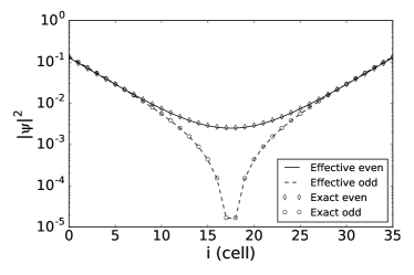
Figure 6: Exponential localization of the $D1/d_{3}$ edge state for $U=3J_{1}$ and $J_{2}=0.1J_{1}$ in a lattice with $36$ unit cells ($72$ sites) in dimerization $D1$. We plot the probability to find two particles in unit cell $i$ calculated with the effective theory in the strong dimerization limit (lines) and with exact diagonalization (markers). Both simulations provide a pair of even and odd almost-degenerate eigenstates due to finite size (see legend).

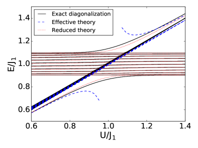
Figure 7: Energy spectrum in dimerization $D2$ at the crossing between the $d_{2}$ bound state and the upper type II continuum for $J_{2}=0.1J_{1}$ and $24$ lattice sites: Exact diagonalization results (black lines), strong dimerization model (blue dashed lines) and reduced model (red dotted lines).

The effective theory fails at $U\sim J_{1}$ because the $D2/d_{2}$ EBS becomes resonant with type II scattering states. In order to account for the hybridization mechanism, we consider a reduced Hilbert space including $d_{2}$-like truncated EBS $-|B_{0},B_{0}\rangle$ and $|A_{L},A_{L}\rangle$, type II scattering states $|\psi^{j}_{i}\rangle=|ES_{j}\rangle\otimes\left(|A_{i}\rangle-|B_{i}\rangle\right)/\sqrt{2}$, where $|ES_{0}\rangle=|B_{0}\rangle$ and $|ES_{L}\rangle=|A_{L}\rangle$ and finally the zero-energy single-particle edge state $|B_{0}A_{L}\rangle$ (see Appendix A.4). This reduced theory reproduces very well the avoided crossing around $U=J_{1}$ (see Fig. 7 (red dotted lines)) and points out that the $D2/d_{2}$ EBS is smoothly transformed into a type II scattering state when moving away from $U\sim J_{1}$.

V Experimental observation and dynamics

In this final section, we present the results of real time simulations which directly highlight the properties of the SSH model discussed in this work. The most promising idea is that, upon the 1D to 2D mapping introduced in Sec. II, a 2D coupled optical fibers setup can provide a quantum simulator of the two-particle 1D SSH model, such that the full two-body dynamics of the system is visibile in real time and real space through the propagating light intensity. Beyond the characterization of scattering, bound and edge bound states as discussed in this section, the same setup would allow the visualization of the closed channel population in a resonant Fano-Feshbach scattering process, already presented in Sec. III.2.

We study the two-body dynamics, assuming different initial conditions at $t=0$ and different interaction strengths $U$. We let the two-body wave function in second quantization evolve numerically in time via exact diagonalization. Written in first quantization, the two-body wavefunction can be interpreted as a single particle wave function $\psi(x,y,t)$ in 2D ($x$ and $y$ being equivalently the coordinates of the two particles in 1D or the coordinates of a single particle in 2D). We address few different illustrative cases, shown in the following subsections.

V.1 Edge bound state $D2/d_{2}$

In Fig. 8(a), we plot the wave function of the exact EBS eigenstate for $U=0.7J_{1}$ and $J_{2}=0.1J_{1}$ in dimerization $D2$ (see Fig. 7). The main components of the EBS wave function are on the diagonal $x=y$ and decay exponentially as $x$ grows. Being even and odd states almost degenerate, one can equally well consider states localized at either end of the lattice. Therefore, as initial state, we take the projection of the exact EBS wave function on $x=y$ with $x\leq 3$, as shown in Fig. 8(b), localized at the bottom left corner of the 2D lattice.

We use the observables $\langle\hat{x}\rangle(t)\equiv\sum_{x}x\,|\psi(x,y,t)|^{2}=\sum_{y}y\,|\psi(x,y,t)|^{2}$ and $\sqrt{\langle(\hat{x}-\hat{y})^{2}\rangle}(t)$ to characterize the edge localization properties of the states. In Fig. 9(a) the time evolution of $\langle\hat{x}\rangle(t)$ is displayed. The plot shows that $\langle\hat{x}\rangle(t)\ll L/2$, namely the initially approximate EBS, remains localized at one edge of the system. It is remarkable that a very well approximated EBS can be obtained by initializing the wave function over only three lattice sites.

However, since the initial state slightly differs from the exact EBS, a small overlap with type II states is present and observed in a non-vanishing single-particle population oscillating at $x=0$ or $y=0$ (see Fig. 9(b)). This produces sizable - but still small when compared to the lattice size - fluctuations $\sqrt{\langle(x-y)^{2}\rangle}$. The visible oscillations in both observables arise from the bouncing of the populated type II states at the lattice edges.

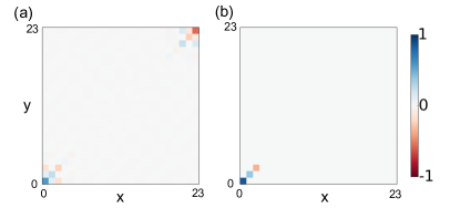
Figure 8: (a) EBS wave function for a lattice with $L=24$ sites in the D2 dimerization for $J_{2}=0.1J_{1}$, $U=0.7J_{1}$ obtained with exact diagonalization. (b) Projected wave function on $x=y$ with $x\leq 3$, used as initial state for the time-evolution shown in Fig. 9(a) and discussed in Sec. V.1.

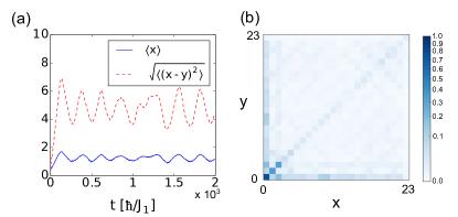
Figure 9: (a) Time evolution of the projected EBS in Fig. 8(b) for dimerization $D2$: $\langle x\rangle$ (full blue line) and $\sqrt{\langle(x-y)^{2}\rangle}$ (dashed red line) as a function of time; (b) Modulus of the two-body wavefunction at $t=10^{3}\hbar/J_{1}$. In these simulations $U=0.7J_{1}$, $J_{2}=0.1J_{1}$ and $L=24$ sites.

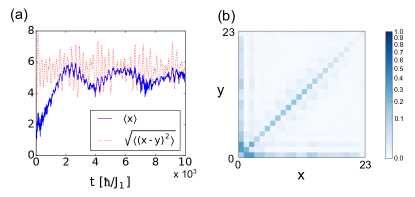
Figure 10: (a) Time evolution of a doublon initially localized at the outermost lattice site for dimerization $D2$: $\langle x\rangle$ (full blue line) and $\sqrt{\langle(x-y)^{2}\rangle}$ (dotted red line) as a function of time; (b) Modulus of the two-body wavefunction at $t=10^{3}\hbar/J_{1}$. In these simulations $U=J_{1}$, $J_{2}=0.1J_{1}$ and $L=24$ sites.

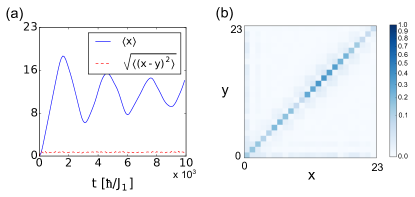
Figure 11: (a) Time evolution of a doublon initially localized in the lattice outer most lattice site for dimerization $D2$: $\langle x\rangle$ (full blue line) and $\sqrt{\langle(x-y)^{2}\rangle}$ (dashed red line) as a function of time; (b) Modulus of the two-body wavefunction at $t=10^{3}\hbar/J_{1}$. In these simulations $U=3J_{1}$, $J_{2}=0.1J_{1}$ and $L=24$ sites.

V.2 Hybridization between $d_{2}$ and type II continuum

Differently from the previous section, we consider as initial condition a single doublon localized at the outermost site of a $D2$ dimerized lattice, and tune the value of interactions to $U=J_{1}$. Such initial state has a sizable overlap with the $D2/d_{2}$ EBS, the $d_{2}$ bound-state continuum and type II scattering states.

The time evolution shows that the state again remains mostly localized at one edge. However, $\langle\hat{x}\rangle(t)$ becomes larger because of the non-negligible population of the $d_{2}$ continuum (see Fig. 10(a)). Moreover, oscillations at two different characteristic time-scales are visible. The fast time scale is present in both observables and it is related to the bouncing of the type II states, as discussed in the previous section. A second slower time-scale is clearly recognizable for the observable $\langle\hat{x}\rangle(t)$ related to the dynamics of the heavy $d_{2}$ bound state and the corresponding bouncing off the lattice edges.

V.3 Bound state dynamics ($D2$)

As initial state, we take again a single doublon localized in the outermost site of a $D2$ dimerized lattice, but increase interactions to move away from the resonance between $d_{2}$ and type II continuum.

At $U=3J_{1}$, this initial state has a large overlap with the $d_{2}$ bound states, which are well localized at $x=y$, but not necessarily at the edges, and negligible overlap with the scattering continua. For that reason, the state delocalizes in the lattice remaining bound at relative distance equal to zero, as shown in Fig. 11. This is reflected in a negligible value of $\sqrt{\langle(x-y)^{2}\rangle}$ during the whole time evolution and a center-of-mass average position of the wave packet oscillating significantly in time due to bounces at the lattice edges.

V.4 Two-body scattering states

As a final example, we show the case where we populate and address scattering states.

We take as initial condition a state delocalized in the first four lattice sites cells without any double occupation. In our notations, the initial state reads differently in the two dimerizations, so that it is convenient to write it explicitly (symmetrization is assumed):

$$|\Psi_{D1}(t=0)\rangle \propto (|A_{1}\rangle+|B_{1}\rangle)\otimes(|A_{2}\rangle+|B_{2}\rangle),$$ (19)

$$|\Psi_{D2}(t=0)\rangle \propto (|B_{0}\rangle+|A_{1}\rangle)\otimes(|B_{1}\rangle+|A_{2}\rangle).$$ (20)

Due to the vanishing double occupation, the energy of the initial state is determined by the hopping processes and not by interactions. It results $E^{(in)}_{\sigma}=-2J_{\sigma}$ depending on the dimerization $D\sigma$ ($\sigma=1,2$). In dimerization $D1$ the initial state lies almost completely in the lower type I scattering continuum, having very small projection on other states. Instead, in dimerzation $D2$, the initial state has non negligible overlap with states in all type I and type II continua.

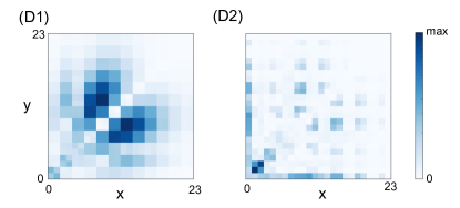
Figure 12: Modulus of the two-body wavefunction after time evolution of the initial states in Eqs. (19, 20) for (D1) dimerization $D1$ and (D2) dimerization $D2$ at time $t=75\hbar/J_{1}$. In these simulations $U=1.5J_{1}$, $J_{2}=0.1J_{1}$ and $L=24$ sites.

For that reason, the time evolution, shown in Fig. 12, presents two drastically different behaviours in the two dimerizations: in $D1$ a two-body scattering pattern develops, which covers the central part of the lattice leaving the density on the diagonal suppressed due to interactions; in $D2$ the two-body wavefunction presents an admixture of two free scattering particles and type II edge-scattering states.

VI Conclusions

In conclusion, we have studied theoretically the rich two-particle physics stemming from the interplay of local interactions with non-trivial single-particle topology. To this aim, we have considered two particles in the paradigmatic one-dimensional Su-Schrieffer-Heeger dimerized lattice. We have proposed an experimentally realistic system, based on state-of-the-art coupled optical fiber technology, where the two-body physics in the SSH model can be quantum simulated in real time and real space. Beyond being able of revealing the different scattering, bound and edge bound states in finite geometries, experiments along the suggested lines have the potential of becoming a textbook illustration of the Fano-Feshbach resonance scattering effect.

One of our major conceptual results resides in the evidence that interactions, in spite of being local, can affect the boundary conditions over more than one single lattice site. Such kind of effects are expected to be even more relevant in the presence of non-local interactions. Hence, the most straightforward extension of the present work regards the inclusion of nearest-neighbor interactions Di Liberto et al. .

Our work provides a first important progress in the understanding of two-body physics in systems with topological properties. In the future, it would be interesting to investigate models in higher dimensions and different geometries, where symmetries other than the chiral one are relevant for the existence of topological states.

VII Acknowledgements

The authors thank M. Burrello, P. Öhberg, C. Ortix, T. Ozawa and H. Price for interesting discussions. A.R. acknowledges support from the Alexander von Humboldt foundation and W. Zwerger for the kind hospitality at the TUM. This work was supported by ERC through the QGBE grant, by the EU-FET Proactive grant AQuS, Project No. 640800 and by Provincia Autonoma di Trento.

Note added. In the final stage of preparation of this work, we became aware of a similar and complementary investigation of the two particle SSH model by Gorlach and Poddubny Gorlach and Poddubny .

Appendix A Effective theories

It this work, we have made extensive use of effective models to describe two bosonic particles in a dimerized lattice governed by the Hamiltonian $H=H_{J_{1}}+H_{J_{2}}+H_{U}$, where $H_{J_{1}}$ and $H_{J_{2}}$ are the strong- and weak-tunneling Hamiltonians, and $H_{U}$ accounts for onsite interactions. In this section, we provide the details of their derivation.

Consider a Hamiltonian $H=H_{0}+V$. Let us label the set of eigenstates of $H_{0}$ as $\{\alpha\}=\{|\alpha,m\rangle\}$. Here, the index $\alpha$ indicates a manifold of states (for instance, states close in energy to each other that are gapped from the rest of the other states), and $m$ labels the states inside the manifold. Be $V$ a perturbation that weakly couples the manifold $\{\alpha\}$ to the manifold $\{\beta\}$ of the remaining eigenstates of $H_{0}$. Including $V$ at second order perturbation theory, as shown in Cohen-Tannoudji et al. (1998), one can obtain an effective Hamiltonian $H^{\alpha}_{\textrm{eff}}$ that describes manifold $\{\alpha\}$

$$\langle\alpha,m|H^{\alpha}_{\textrm{eff}}|\alpha,n\rangle=E_{\alpha,m}\delta_{m,n}+\langle\alpha,m|V|\alpha,n\rangle+$$ (21)

$$+\frac{1}{2}\sum_{k,\beta\neq\alpha}\langle\alpha,m|V|\beta,k\rangle\langle\beta,k|V|\alpha,n\rangle\times$$

$$\times\left[\frac{1}{E_{\alpha,m}-E_{\beta,k}}+\frac{1}{E_{\alpha,n}-E_{\beta,k}}\right]\,,$$

where $E_{\alpha,m}$ are the eigenvalues of $H_{0}$ relative to the eigenstate $|\alpha,m\rangle$.

A.1 Strong dimerization

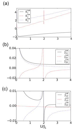
Figure 13: Bulk parameters $E^{\textrm{bulk}}_{\alpha}$ and $J^{\textrm{bulk}}_{\alpha\beta}$ of the effective model in Eq. (30) for $J_{2}=0.1J_{1}$, as a function of $U$. The detailed legend can be found in the figure.

In the limit of strong dimerization $J_{2}\ll J_{1},U$, we identify $H_{0}=H_{J_{1}}+H_{U}=\sum_{i}H^{\textrm{cell}}_{i}$. Different lattice cells are decoupled and each cell is described by the strong-link Hamiltonian $H^{\textrm{cell}}_{i}$, which in the two-particles basis $|A_{i},A_{i}\rangle$, $|A_{i},B_{i}\rangle$ and $|B_{i},B_{i}\rangle$ takes the form

$$H^{\textrm{cell}}_{i}=\begin{pmatrix}U&-\sqrt{2}J_{1}&0\\ -\sqrt{2}J_{1}&0&-\sqrt{2}J_{1}\\ 0&-\sqrt{2}J_{1}&U\end{pmatrix}\,.$$ (22)

Its eigenvectors, provided in Eqs. (3-5), have respectively energy

$$\epsilon_{1} = \frac{1}{2}\left(U-\sqrt{16J_{1}^{2}+U^{2}}\right),$$ (23)

$$\epsilon_{2} = U,$$ (24)

$$\epsilon_{3} = \frac{1}{2}\left(U+\sqrt{16J_{1}^{2}+U^{2}}\right).$$ (25)

The states in manifold $\{\alpha\}=\{|d_{1,i}\rangle,|d_{2,i}\rangle,|d_{3,i}\rangle\}$ are coupled through $H_{J_{2}}$ in a non-trivial manner via the manifold of virtual states $\{\beta\}$ - also eigenstates of $H_{0}$. For PBC, manifold $\{\beta\}$ is formed by states of one particle in a cell $i$ and one particle in a cell $j$, with $i\neq j$. There are four possible sets of states

$$|\psi^{I}_{ij}\rangle =\frac{1}{\sqrt{2}}\left(|A_{i}\rangle+|B_{i}\rangle\right)\otimes\frac{1}{\sqrt{2}}\left(|A_{j}\rangle+|B_{j}\rangle\right)\,,$$ (26)

$$|\psi^{II}_{ij}\rangle =\frac{1}{\sqrt{2}}\left(|A_{i}\rangle-|B_{i}\rangle\right)\otimes\frac{1}{\sqrt{2}}\left(|A_{j}\rangle-|B_{j}\rangle\right)\,,$$ (27)

$$|\psi^{III}_{ij}\rangle =\frac{1}{\sqrt{2}}\left(|A_{i}\rangle+|B_{i}\rangle\right)\otimes\frac{1}{\sqrt{2}}\left(|A_{j}\rangle-|B_{j}\rangle\right)\,,$$ (28)

$$|\psi^{IV}_{ij}\rangle =\frac{1}{\sqrt{2}}\left(|A_{i}\rangle-|B_{i}\rangle\right)\otimes\frac{1}{\sqrt{2}}\left(|A_{j}\rangle+|B_{j}\rangle\right)\,,$$ (29)

with energies, respectively, $E^{I}=-2J_{1}$, $E^{II}=2J_{1}$, $E^{III}=E^{IV}=0$. Up to second order in perturbation $V=H_{J_{2}}$, one finds the effective Hamiltonian (see Eq. (18))

$$H_{\textrm{eff}}=\sum_{i,\alpha}E_{\alpha,i}\,d^{\dagger}_{\alpha,i}d_{\alpha,i}+\sum_{\langle i,j\rangle}\sum_{\alpha,\beta}J_{\alpha\beta}^{ij}\,d^{\dagger}_{\alpha,i}d_{\beta,j}\,,$$ (30)

containing renormalized onsite dimer energies and intra- and inter-dimer nearest-neighbor hopping. In general, coefficients $E_{\alpha,i}$ and $J_{\alpha\beta}^{ij}$ have a quite involved analytical form. The values of the parameters for $J_{2}=0.1J_{1}$ as a function of $U$ are shown in Fig. 13 when $\langle i,j\rangle$ are in the bulk of the lattice where no edge effects are involved. The divergencies at $U=2J_{1}$ are the indication of the crossing of $d_{2}$ with the higher type I continuum.

In most regimes, the different bound states are far away in energy from each other and the coupling among them turns out to be weak. Even if better quantitative predictions for the bound states bands can be obtained by including all the terms, a decoupling of the different bound states, namely considering for each bound state $d_{\alpha}$ only the parameters $J_{\alpha\alpha}^{ij}$ and $E_{\alpha,i}$, still provides an excellent agreement. In that case, explicit analytical forms can be provided at least for the simpler case of state $d_{2}$:

$$J_{22}^{\textrm{bulk}} =-\frac{J_{2}^{2}}{U}\frac{2J_{1}^{2}-U^{2}}{4J_{1}^{2}-U^{2}}\,,$$ (31)

$$E_{2}^{\textrm{bulk}} =U-2J_{22}^{\textrm{bulk}}\,.$$ (32)

For OBC, bulk and edge parameters differ: in $D1$, due to the missing coupling either on the right-hand or left-hand side, one gets a different renormalization of the onsite energy at the first and last cells:

$$E_{2}^{\textrm{edge,D1}}=U-J_{22}^{\textrm{bulk}}\,,$$ (33)

while the effective hopping parameter is equal at the edges as in the bulk.

Different parameters describe dimerization $D2$, due to the presence of half cells (single lattice sites) at the chain edges. The effective tunneling coupling between the first (last) lattice site to the first (last) complete lattice cell and the energy offset of the first (last) lattice sites are

$$J_{22}^{\textrm{edge,D2}} = \frac{J_{2}^{2}}{U}\frac{\sqrt{2}U^{2}}{J_{1}^{2}-U^{2}}\,,$$ (34)

$$E_{2}^{\textrm{edge,D2}} = U-\sqrt{2}J_{22}^{\textrm{edge,D2}}\,.$$ (35)

Finally, the first ($i=1$) and last ($i=L-1$) complete cells feel a resulting energy shift given by

$$E_{2,1}=E_{2,L-1}=U+\frac{J_{2}^{2}}{U}\frac{2J_{1}^{4}-7J_{1}^{2}U^{2}+2U^{4}}{4J_{1}^{4}-5J_{1}^{2}U^{2}+U^{4}}\,.$$ (36)

A.2 Strong-interaction limit

In the strong-interaction limit $U\gg J_{1},J_{2}$, the two $d_{2,3}$ narrow bound-state bands are well separated from the rest of the spectrum, as one can deduce from Eqs. (24,25) and Figs. 5(D1,D2). We choose linear combinations of these higher repulsive bound states to constitute the manifold $\{\alpha\}$ for which we write the effective theory. This corresponds to consider $H_{0}=H_{U}$ and the subspace of onsite doublons $\{\alpha\}=\{|A_{i},A_{i}\rangle,|B_{i},B_{i}\rangle\}\equiv\{d_{A,i}^{\dagger}|0\rangle,d_{B,i}^{\dagger}|0\rangle\}$, with energy $E_{\alpha}=U$.

The virtual states at energy $E_{\beta}=0$ form manifold $\{\beta\}=\{|A_{i},A_{j}\rangle,|B_{i},B_{j}\rangle\,|A_{m},B_{n}\rangle\}$ with $i\neq j$ and $\forall m,n$. The coupling is provided by $V=H_{J_{1}}+H_{J_{2}}$. Up to second order in $J_{\sigma}$, only $|A_{i},B_{i}\rangle$ and $|A_{i},B_{i-1}\rangle$ contribute, corresponding to nearest-neighbor virtual hopping processes.

One obtains an effective single-particle Hamiltonian for the on-site doublons that reads

$$H_{\textrm{eff}}= \frac{2J_{1}^{2}}{U}\sum_{i}d^{\dagger}_{A,i}d_{B,i}+\frac{2J_{2}^{2}}{U}\sum_{i}d^{\dagger}_{A,i+1}d_{B,i}+\textrm{H.c.}$$

$$+\left[U+\frac{2}{U}\left(J_{1}^{2}+J_{2}^{2}\right)\right]\sum_{i}\left(d^{\dagger}_{A,i}d_{A,i}+d^{\dagger}_{B,i}d_{B,i}\right)\,.$$ (37)

The first line clearly shows that the effective model of the bound states is a SSH model with renormalized hopping coefficients

$$J_{1,2}^{\textrm{eff}}=-\frac{2J_{1,2}^{2}}{U}\,$$ (38)

and effective on-site energies

$$\epsilon_{\textrm{bulk}}=U+\frac{2}{U}\left(J_{1}^{2}+J_{2}^{2}\right)\,,$$ (39)

which contains the binding energy $U$ and an on-site energy shift. The latter is generated by similar second-order processes as the ones occurring for the hopping terms: a virtual breaking of the doublon to the left and to the right. However, in the presence of OBC, at the edges only one of these two processes will be present, leading to a different on-site energy at the edge with respect to the bulk

$$\epsilon_{\textrm{edge}}=\epsilon_{\textrm{bulk}}+\Delta E_{\sigma},$$ (40)

with $\Delta E_{\sigma}=-2J_{3-\sigma}^{2}/U$, depending on the dimerization $D\sigma$ (with $\sigma=1,2$).

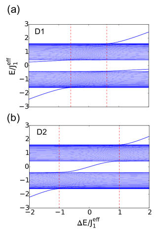
Figure 14: Single-particle SSH spectrum of a finite chain with $48$ sites for $J^{\textrm{eff}}_{2}=0.6J^{\textrm{eff}}_{1}$ as a function of an arbitrary on-site energy shift $\Delta E$ for (a) dimerization $D1$ and (b) dimerization $D2$. As discussed in the text, this single-particle model effectively describes the bound-states physics in the strong-interaction limit. The red lines are the critical values of $\Delta E$ for the existence of Tamm or in-gap edge states (see text).

This effective Hamiltonian provides a generalization of the Tamm physics to the SSH model, which is summarized in Fig. 14. For varying $\Delta E$, the energy of the Tamm-like states lies above/below the bands and it depends linearly on $\Delta E$ when $|\Delta E|$ is sufficiently large. They appear for $|\Delta E|>J_{2}^{\textrm{eff}}$ in dimerization $D1$ and for $|\Delta E|>J_{1}^{\textrm{eff}}$ in dimerization $D2$. In-gap states between the bands appear for both dimerizations, but they exist in $D1$ when $|\Delta E|>J_{2}^{\textrm{eff}}$ and in $D2$ when $|\Delta E|<J_{1}^{\textrm{eff}}$.

The in-gap edge states obtained when considering $\Delta E$ as tunable parameter, have a topological origin. The peculiar feature of the SSH model is indeed the presence of zero-energy edge states in dimerization $D2$ that are topologically protected by chiral symmetry. However, chiral symmetry is broken by the presence of the off-set $\Delta E$, as proven below. As a consequence, topological edge states in $D2$ are not protected anymore and, for moderate $\Delta E$, shift away from zero energy, as discussed in the paragraph above and shown in Fig. 14(b). Also the in-gap states in dimerization $D1$ have a similar topological origin. Indeed, one can observe from Fig. 14(a) that these states asympotically tend to zero energy for infinitely large values of $\Delta E$. In this limit, the system behaves as an ideal $D2$ dimerized lattice with $L-2$ sites, which must possess zero-energy edge states.

In the specific case of the effective model derived in this section, we have found that $|\Delta E_{1}|=J_{2}^{\textrm{eff}}$ and $|\Delta E_{2}|=J_{1}^{\textrm{eff}}$, which implies that we are exactly at the critical values of $\Delta E$ (red lines in Fig. 14) for which neither Tamm nor in-gap states can exist.

We now prove the breaking of chiral symmetry in the effective model. Let us consider a finite chain with $2L$ sites in dimerization $D2$. This corresponds to $L-1$ full cells and two single lattice sites at the boundaries. After defining the vector $\mathbf{d}=(d_{A,1},\dots,d_{A,L},d_{B,0},\dots,d_{B,L-1}$), the Hamiltonian takes the form (up to an overall irrelevant energy shift that we drop in the discussion below)

$$H_{\textrm{eff}}=\mathbf{d}^{\dagger}\mathcal{H}_{\textrm{eff}}\mathbf{d}=\mathbf{d}^{\dagger}\left(\begin{array}[]{cc}\mathcal{H}_{11}&\mathcal{H}_{12}\\ \mathcal{H}_{12}^{\dagger}&\mathcal{H}_{22}\end{array}\right)\mathbf{d}\,.$$ (41)

While $\mathcal{H}_{12}$ is a $L\times L$ matrix that contains the coupling between neighboring sites and has the form

$$\mathcal{H}_{12}=\left(\begin{array}[]{ccccc}-J_{1}^{\textrm{eff}}&&&&0\\[6.0pt] -J_{2}^{\textrm{eff}}&-J_{1}^{\textrm{eff}}&&&\\ &\ddots&\ddots&&\\ &&\ddots&-J_{1}^{\textrm{eff}}&\\[6.0pt] 0&&&-J_{2}^{\textrm{eff}}&-J_{1}^{\textrm{eff}}\end{array}\right)\,,$$ (42)

$\mathcal{H}_{11}$ and $\mathcal{H}_{22}$ are $L\times L$ diagonal matrices, namely $\mathcal{H}_{11}=\textrm{diag}(0,\cdots,0,\Delta E_{2})$ and $\mathcal{H}_{22}=\textrm{diag}(\Delta E_{2},0,\cdots,0)$ that describe the on-site energy shift, respectively, of the left and right edge of the chain. If $\Delta E_{2}$ were zero, the diagonal blocks $\mathcal{H}_{11}$ and $\mathcal{H}_{22}$ would vanish. Hence, the Hamiltonian could be written in the chiral-symmetric form $\mathcal{H}_{\textrm{eff}}^{(0)}=\begin{pmatrix}\mathbf{0}&\mathcal{H}_{12}\\ \mathcal{H}_{12}^{\dagger}&\mathbf{0}\end{pmatrix}$. In fact, in this case, the operator $\mathcal{C}=\sigma_{z}\otimes\mathcal{I}$ provides a chiral symmetry such that $\{\mathcal{H}_{\textrm{eff}}^{(0)},\mathcal{C}\}=0$. However, since in our case $\Delta E_{2}\neq 0$, diagonal blocks appear in $\mathcal{H}_{\textrm{eff}}$. Chiral symmetry is therefore broken and zero-energy edge states are not protected Ryu and Hatsugai (2002).

A.3 Effective theory for the $d_{NN}$ state

We develop an effective theory in the strong-dimerization limit $J_{2}\ll J_{1}$ to qualitative explain the existence of the $d_{NN}$ bound state. The basis for the effective theory is given by the subspace of states $|S_{ij}\rangle\sim(|A_{i}\rangle-|B_{i}\rangle)\otimes(|A_{j}\rangle-|B_{j}\rangle)$ with $i$, $j$ arbitrary cell indices. For $i\neq j$, the states $|S_{ij}\rangle$ span the upper type I scattering continuum. For $i=j$, $|S_{ii}\rangle=(|d_{3}(U=0)\rangle$, which can be considered a fairly good approximation for $d_{3}$ up to $U\leq 2J_{1}$. At first order in $J_{2}$, the energies of states $|S_{ij}\rangle$ are $E_{ij}=2J_{1}+\delta_{ij}U/2$. The single-particle hopping amplitude in this subspace is given by $J_{2}/2$. When $U$ is approaching $2J_{1}$ (but sufficiently far to be off-resonant with the type I scattering states), state $d_{2}$ become closer in energy to the $S_{ij}$ manifold. Then, the energy of the states $|S_{ij}\rangle$ with $i=j\pm 1$ is not simply given by $2J_{1}$ but it is renormalized by second-order processes mediated by the virtual state $d_{2}$. The energy shift is given by

$$\Delta E_{NN}=2\times\frac{J_{2}^{2}}{4}\frac{1}{2J_{1}-U}$$ (43)

and provides an effective nearest-neighbor attractive (repulsive) interaction when $U>2J_{1}$ ($U<2J_{1}$). Therefore, for $U>2J_{1}$ ($U<2J_{1}$) we expect a bound state above (below) the continuum. The nearest-neighbor interaction is very weak compared to the bandwidth $2J_{2}$ of the scattering states. This explains the appearance of the $d_{NN}$ state for a limited set of momenta close to $K=\pi$ Valiente and Petrosyan (2009). Moreover, for increasing values of $U$ the attraction becomes weaker and weaker, leading to a progressive disappearance of the $d_{NN}$ state. These properties have all been observed numerically (see Fig. 2(a-b)).

A.4 Reduced theory for the avoided crossing

Using the formalism presented in A.1, we were able to describe the narrow bound states bands. However, the hybridization between bound states and type I scattering states presented in Fig. 7 has to be accounted for with a different model, including type II scattering states as real rather than virtual states.

The Hilbert space of the reduced theory for the avoided crossing is provided by the set of states $\{|\psi^{\textrm{red}}\rangle\}=\{|d_{2,0}\rangle\,,|\psi^{l}_{i}\rangle\,,|\psi^{\textrm{loc}}\rangle\,,|\psi^{r}_{i}\rangle\,,|d_{2,L}\rangle\}$:

$$|d_{2,0}\rangle =-|B_{0},B_{0}\rangle\,,$$

$$|\psi^{l}_{i}\rangle =|B_{0}\rangle\otimes\left(|A_{i}\rangle-|B_{i}\rangle\right)/\sqrt{2}\quad i=1,\cdots,L-1\,,$$

$$|\psi^{\textrm{loc}}\rangle =|B_{0}A_{L}\rangle\,,$$

$$|\psi^{r}_{i}\rangle =|A_{L}\rangle\otimes\left(|A_{i}\rangle-|B_{i}\rangle\right)/\sqrt{2}\quad i=1,\cdots,L-1\,,$$

$$|d_{2,L}\rangle =|A_{L},A_{L}\rangle\,.$$

One therefore constructs the reduced Hamiltonian

$$\langle\psi^{\textrm{red}}_{\alpha}|\mathcal{H}^{\textrm{red}}|\psi^{\textrm{red}}_{\beta}\rangle\equiv\langle\psi^{\textrm{red}}_{\alpha}|H|\psi^{\textrm{red}}_{\beta}\rangle,$$ (44)

that reads

$$\mathcal{H}^{\textrm{red}}=\left(\begin{array}[]{c|ccccc|c|ccccc|c}U&J_{2}&&&&&&&&&&&\\ \hline\cr J_{2}&J_{1}&-\frac{J_{2}}{2}&&&&&&&&&&\\ &-\frac{J_{2}}{2}&J_{1}&\ddots&&&&&&&&&\\[0.0pt] &&\ddots&\ddots&\ddots&&&&&&&&\\[0.0pt] &&&\ddots&J_{1}&-\frac{J_{2}}{2}&&&&&&&\\[0.0pt] &&&&-\frac{J_{2}}{2}&J_{1}&\frac{J_{2}}{\sqrt{2}}&&&&&&\\ \hline\cr&&&&&\frac{J_{2}}{\sqrt{2}}&0&-\frac{J_{2}}{\sqrt{2}}&&&&&\\ \hline\cr&&&&&&-\frac{J_{2}}{\sqrt{2}}&J_{1}&-\frac{J_{2}}{2}&&&&\\ &&&&&&&-\frac{J_{2}}{2}&J_{1}&\ddots&&&\\ &&&&&&&&\ddots&\ddots&\ddots&&\\ &&&&&&&&&\ddots&J_{1}&-\frac{J_{2}}{2}&\\ &&&&&&&&&&-\frac{J_{2}}{2}&J_{1}&J_{2}\\ \hline\cr&&&&&&&&&&&J_{2}&U\end{array}\right)\,.$$ (45)

The diagonalization of $H^{\textrm{red}}$ shows a very good agreement with the complete spectrum obtained by exact diagonalization, as shown in Fig. 7.

References

- Hubbard (1963) J. Hubbard, Proceedings of the Royal Society of London A: Mathematical, Physical and Engineering Sciences 276, 238 (1963).
- Mattis (1986) D. C. Mattis, Rev. Mod. Phys. 58, 361 (1986).
- Winkler et al. (2006) K. Winkler, G. Thalhammer, F. Lang, R. Grimm, J. Hecker Denschlag, A. J. Daley, A. Kantian, H. P. Büchler, and P. Zoller, Nature 441, 853 (2006).
- Valiente and Petrosyan (2009) M. Valiente and D. Petrosyan, Journal of Physics B: Atomic, Molecular and Optical Physics 42, 121001 (2009).
- Valiente (2010) M. Valiente, Phys. Rev. A 81, 042102 (2010).
- Longhi (2012) S. Longhi, Phys. Rev. B 86, 075144 (2012).
- Nygaard et al. (2008) N. Nygaard, R. Piil, and K. Mølmer, Phys. Rev. A 78, 023617 (2008).
- Valiente and Mølmer (2011) M. Valiente and K. Mølmer, Phys. Rev. A 84, 053628 (2011).
- Valiente et al. (2010) M. Valiente, M. Küster, and A. Saenz, EPL (Europhysics Letters) 92, 10001 (2010).
- Menotti et al. (2016) C. Menotti, F. Minganti, and A. Recati, Phys. Rev. A 93, 033602 (2016).
- Strohmaier et al. (2010) N. Strohmaier, D. Greif, R. Jördens, L. Tarruell, H. Moritz, T. Esslinger, R. Sensarma, D. Pekker, E. Altman, and E. Demler, Phys. Rev. Lett. 104, 080401 (2010).
- Schreiber et al. (2015) M. Schreiber, S. S. Hodgman, P. Bordia, H. P. Lüschen, M. H. Fischer, R. Vosk, E. Altman, U. Schneider, and I. Bloch, Science 349, 842 (2015).
- Barbiero et al. (2015) L. Barbiero, C. Menotti, A. Recati, and L. Santos, Phys. Rev. B 92, 180406 (2015).
- Tamm (1932) I. Tamm, Phys. Z. Soviet Union. 1, 733 (1932).
- Shockley (1939) W. Shockley, Phys. Rev. 56, 317 (1939).
- Hasan and Kane (2010) M. Z. Hasan and C. L. Kane, Rev. Mod. Phys. 82, 3045 (2010).
- (17) D. Tong, arXiv:1606.06687 .
- Tsui et al. (1982) D. C. Tsui, H. L. Stormer, and A. C. Gossard, Phys. Rev. Lett. 48, 1559 (1982).
- Laughlin (1983) R. B. Laughlin, Phys. Rev. Lett. 50, 1395 (1983).
- Longhi (2011) S. Longhi, Opt. Lett. 36, 3248 (2011).
- Corrielli et al. (2013) G. Corrielli, A. Crespi, G. Della Valle, S. Longhi, and R. Osellame, Nature Communications 4, 1555 (2013).
- Schreiber et al. (2012) A. Schreiber, A. Gábris, P. P. Rohde, K. Laiho, M. Štefaňák, V. Potoček, C. Hamilton, I. Jex, and C. Silberhorn, Science 336, 55 (2012).
- Mukherjee et al. (2015) S. Mukherjee, A. Spracklen, D. Choudhury, N. Goldman, P. Öhberg, E. Andersson, and R. R. Thomson, New Journal of Physics 17, 115002 (2015).
- Mukherjee et al. (2016) S. Mukherjee, M. Valiente, N. Goldman, A. Spracklen, E. Andersson, P. Öhberg, and R. R. Thomson, Phys. Rev. A 94, 053853 (2016).
- Ryu and Hatsugai (2002) S. Ryu and Y. Hatsugai, Phys. Rev. Lett. 89, 077002 (2002).
- Zak (1989) J. Zak, Phys. Rev. Lett. 62, 2747 (1989).
- Atala et al. (2013) M. Atala, M. Aidelsburger, J. T. Barreiro, D. Abanin, T. Kitagawa, E. Demler, and I. Bloch, Nat. Phys. 9, 795 (2013).
- Chiu et al. (2016) C.-K. Chiu, J. C. Y. Teo, A. P. Schnyder, and S. Ryu, Rev. Mod. Phys. 88, 035005 (2016).
- Grusdt et al. (2013) F. Grusdt, M. Höning, and M. Fleischhauer, Phys. Rev. Lett. 110, 260405 (2013).
- Deng and Santos (2014) X. Deng and L. Santos, Phys. Rev. A 89, 033632 (2014).
- Pinto et al. (2009) R. A. Pinto, M. Haque, and S. Flach, Phys. Rev. A 79, 052118 (2009).
- Bello et al. (2016) M. Bello, C. E. Creffield, and G. Platero, Scientific Reports 6, 22562 (2016).
- Note (1) See, for instance, Ref. Qin et al. for a generalization of topological invariants to multiparticle systems.
- Hsu et al. (2016) C. W. Hsu, B. Zhen, A. D. Stone, J. D. Joannopoulos, and M. Soljačić, Nature Reviews Materials 1, 16048 EP (2016).
- Della Valle and Longhi (2014) G. Della Valle and S. Longhi, Phys. Rev. B 89, 115118 (2014).
- (36) M. Di Liberto, A. Recati, I. Carusotto, and C. Menotti, ArXiv:1612.02601.
- (37) M. A. Gorlach and A. N. Poddubny, arXiv:1608.02093 .
- Cohen-Tannoudji et al. (1998) C. Cohen-Tannoudji, J. Dupont-Roc, and G. G. Grynberg, Atom-Photon Interactions: Basic Processes and Applications (John Wiley Sons, Inc., 1998).
- (39) X. Qin, F. Mei, F. Ke, L. Zhang, and C. Lee, ArXiv:1611.00205, (2016).