Influence of external potentials on heterogeneous diffusion processes

Abstract

In this paper we consider heterogeneous diffusion processes with the power-law dependence of the diffusion coefficient on the position and investigate the influence of external forces on the resulting anomalous diffusion. The heterogeneous diffusion processes can yield subdiffusion as well as superdiffusion, depending on the behavior of the diffusion coefficient. We assume that not only the diffusion coefficient but also the external force has a power-law dependence on the position. We obtain analytic expressions for the transition probability in two cases: when the power-law exponent in the external force is equal to $2\eta-1$, where $2\eta$ is the power-law exponent in the dependence of the diffusion coefficient on the position, and when the external force has a linear dependence on the position. We found that the power-law exponent in the dependence of the mean square displacement on time does not depend on the external force, this force changes only the anomalous diffusion coefficient. In addition, the external force having the power-law exponent different from $2\eta-1$ limits the time interval where the anomalous diffusion occurs. We expect that the results obtained in this paper may be relevant for a more complete understanding of anomalous diffusion processes.

I Introduction

There are many systems and processes where the time dependence of the centered second moment is not linear as in the classical Brownian motion. Such family of processes is called anomalous diffusion. In one dimension the anomalous diffusion is characterized by the power-law time dependence of the mean square displacement (MSD) Bouchaud and Georges (1990)

$$\langle(\Delta x)^{2}\rangle=K_{\alpha}t^{\alpha}\,.$$ (1)

Here $K_{\alpha}$ is the anomalous diffusion coefficient. When $\alpha\neq 1$, this time dependence deviates from the linear function of time characteristic for the Brownian motion. If $\alpha<1$, the phenomenon is called subdiffusion. Occurrence of subdiffusion has been experimentally observed, for example, in the behavior of individual colloidal particles in two-dimensional random potential energy landscapes Evers et al. (2013). It has been theoretically shown that active particles moving at constant speed in a heterogeneous two-dimensional space experience self trapping leading to subdiffusion Chepizhko and Peruani (2013). Usually it is assumed that subdiffusive behavior is caused by the particle being trapped in local minima for prolonged times before it escapes to a neighboring minima. Continuous time random walks (CTRWs) with on-site waiting-time distributions falling slowly as $t^{-\alpha-1}$ predict a subdiffusive behavior Metzler and Klafter (2000); Schubert et al. (2013).

Superdiffusion processes, characterized by the nonlinear dependence (1) of the MSD on time with the power-law exponent in the range $1<\alpha<2$, constitute another subclass of anomalous diffusion processes. Superdiffusion is observed, for example, in vibrated dense granular media Scalliet et al. (2015). Theoretical models suggest that supperdiffusion can be caused by Lévy flights Metzler and Klafter (2000). Lévy flights resulting in a superdiffusion can be modeled by fractional Fokker-Planck equations Fogedby (1994) (or Langevin equations with an additive Lévy stable noise). In many experimental studies it is only possible to show that signal intensity distribution has Lévy law-tails: distribution function of turbulent magnetized plasma emitters Marandet et al. (2003) and step-size distribution of photons in hot vapors of atoms Mercadier et al. (2009) have Lévy tails. This indirectly shows that in these systems superdiffusion could be found.

Anomalous diffusion does not uniquely indicate the processes occurring in the system, because there are different stochastic processes sharing the behavior of the MSD (1). The physical mechanisms leading to the deviations from the linear time dependence of the MSD can depend on the system or on the temporal and spatial ranges under consideration. For example, diffusion described by CTRW has been observed for sub-micron tracers in biological cells Tabei et al. (2013); Weigel et al. (2011); Jeon et al. (2011), structured coloidal systems Wong et al. (2004) and for charge carrier motion in amorphous semiconductors Scher and Montroll (1975); Schubert et al. (2013). Fractional Brownian motion and fractional Langevin equations has been used to model the dynamics in membranes Jeon et al. (2012); Kneller et al. (2011), motion of polymers in cells Kepten et al. (2013), tracer motion in complex liquids Szymanski and Weiss (2009); Jeon et al. (2013). Diffusion of even smaller tracers in biological cells has been described by a spatially varying diffusion coefficient Kühn et al. (2011).

Recently, in Refs. Cherstvy et al. (2013); Cherstvy and Metzler (2013); Cherstvy et al. (2014a); Cherstvy and Metzler (2014) it was suggested that the anomalous diffusion can be a result of heterogeneous diffusion process (HDP), where the diffusion coefficient depends on the position. Spatially dependent diffusion can occur in heterogeneous systems. For example, heterogeneous medium with steep gradients of the diffusivity can be created in thermophoresis experiments using a local variation of the temperature Maeda et al. (2012); Mast et al. (2013). Mesoscopic description of transport in heterogeneous porous media in terms of space dependent diffusion coefficients is used in hydrology Haggerty and Gorelick (1995); Dentz and Bolster (2010). In turbulent media the Richardson diffusion has been described by heterogeneous diffusion processes Richardson (1926). Power-law dependence of the diffusion coefficient on the position has been proposed to model diffusion of a particle on random fractals O’Shaughnessy and Procaccia (1985); Loverdo et al. (2009). In bacterial and eukaryotic cells the local cytoplasmic diffusivity has been demonstrated to be heterogeneous English et al. (2011); Kühn et al. (2011). Motion of a Brownian particle in an environment with a position dependent temperature has been investigated in Ref. Kazakevičius and Ruseckas (2015). In random walk description the spatially varying diffusion coefficient can be included via position dependence of the waiting time for a jump event Srokowski (2014), the position dependence occurs because in the heterogeneous medium the properties of a trap can reflect the medium structure. This is the case for diffusion on fractals and multifractals Schertzer et al. (2001). Inhomogeneous versions of continuous time random walk models for water permeation in porous ground layers were proposed in Ref. Dentz et al. (2012). Heterogeneous diffusion process might be applicable to describe anomalous diffusion in such systems.

The goal of this paper is to consider HDPs with the power-law dependence of the diffusion coefficient on the position and to analytically investigate the influence of external forces on the resulting anomalous diffusion. The influence of the external forces on HDPs has not been systematically analyzed. In this paper we assume that the forces are characterized by a power-law dependence on the position. Such forces can arise in various systems: In many cases the potentials causing the deterministic forces are power-law functions of position, for example linear and harmonic potentials. Power-law potential with arbitrary power-law exponent acting on a nanoparticle have been created in Ref. Cohen (2005). Logarithmic potentials yielding forces behaving as $x^{-1}$ have been applied to describe dynamics of particles near a long, charged polymer Manning (1969), momentum diffusion in dissipative optical lattices Sagi et al. (2012), long-range interacting systems Bouchet and Dauxois (2005), bubbles in DNA molecules Wu et al. (2009). As we demonstrate, the external force having a certain value of the power-law exponent does not restrict the region of diffusion and change only the anomalous diffusion coefficient without changing the scaling exponent $\alpha$. Other values of the power-law exponent in the external force can lead to the exponential cut-off of the probability density function (PDF) and restrict the region of diffusion, limiting the time interval when the anomalous diffusion occurs. We expect that the results obtained in this paper may be relevant for a more complete understanding of anomalous diffusion processes.

The paper is organized as follows: In Sec. II we summarize the main properties of HDPs with the power-law dependence of the diffusion coefficient on the position. The influence of an external force with a particular value of the power-law exponent is investigated in Sec. III. This value of the power-law exponent is the same as in the drift correction for transformation from the Stratonovich to the Itó stochastic equation. We consider external forces having other values of the power-law exponent in Sec. IV. Sec. V summarizes our findings.

II Free heterogeneous diffusion process

Heterogeneous diffusion process with the power-law dependence of the diffusion coefficient on the position, introduced in Ref. Cherstvy et al. (2013), is described by the Langevin equation

$$dx=\sigma|x|^{\eta}\circ dW_{t}\,.$$ (2)

Here $\eta$ is the power-law exponent of multiplicative noise, $\sigma$ is the amplitude of noise and $W_{t}$ is a standard Wiener process (Brownian motion). This stochastic differential equation (SDE) is interpreted in Stratonovich sense. For mathematical convenience and for further generalization we transform Eq. (2) to the Itô convention:

$$dx=\frac{1}{2}\sigma^{2}\eta|x|^{2(\eta-1)}xdt+\sigma|x|^{\eta}dW_{t}\,.$$ (3)

The Fokker-Planck equation corresponding to the SDE (2) is Gardiner (2004)

$$\frac{\partial}{\partial t}P(x,t)=\frac{1}{2}\sigma^{2}\frac{\partial}{\partial x}\left[|x|^{\eta}\frac{\partial}{\partial x}\left(|x|^{\eta}P(x,t)\right)\right]\,.$$ (4)

With the reflective boundaries at small positive $x=x_{\mathrm{min}}$ and large $x=x_{\mathrm{max}}$, Eq. (4) leads to the steady-state PDF $P_{0}(x)\sim x^{-\eta}$. Without such boundaries the time-dependent solution of Eq. (4) with the initial condition $P(x,0)=\delta(x)$ is given by a stretched (when $\eta>0$) or compressed (when $\eta<0$) Gaussian Cherstvy et al. (2013)

$$P(x,t)=\frac{|x|^{-\eta}}{\sqrt{2\pi\sigma^{2}t}}\exp\left(-\frac{|x|^{2(1-\eta)}}{2(1-\eta)^{2}\sigma^{2}t}\right)\,.$$ (5)

When $\eta<1$, this solution describes exponential cut-off at large values of $x$ and power-law behavior at small values of $x$. The position of the cut-off moves towards large values of $x$ with increase of time $t$. In contrast, when $\eta>1$ the solution (5) describes exponential cut-off at small values of $x$ and power-law behavior at large values of $x$. The position of cut-off moves towards smaller values of $x$ with increase of time $t$.

In Ref. Cherstvy et al. (2013) it has been demonstrated that Eq. (2) (or, equivalently, Eq. (3)) leads to the power-law time dependence of the MSD

$$\langle x^{2}(t)\rangle\sim(\sigma^{2}t)^{\frac{1}{1-\eta}}\,.$$ (6)

This behavior of the MSD means that HDP described by Eq. (2) yields superdiffusion for $1>\eta>0$ and subdiffusion for $\eta<0$. For $\eta>0$ the diffusivity increases with increasing $x$, leading to a progressive acceleration of the diffusing particle. In contrast, the diffusivity decreases with increasing $x$ when $\eta<0$. For $\eta>1$ the particle becomes localized. When $\eta=1$, the MSD grows not as a power-law of time, but exponentially Lau and Lubensky (2007); Fuliński (2011).

The HDP (2) displays weak non-ergodicity, that is the scaling of time and ensemble averages is different. Specifically, in Ref. Cherstvy et al. (2013) it has been shown that the average over the trajectories

$$\left\langle\overline{\delta^{2}(\Delta)}\right\rangle=\frac{1}{N}\sum_{i=1}^{N}\overline{\delta_{i}^{2}(\Delta)}$$ (7)

of the the time-averaged MSD

$$\overline{\delta^{2}(\Delta)}=\frac{1}{T-\Delta}\int_{0}^{T-\Delta}[x(t+\Delta)-x(t)]^{2}dt$$ (8)

scales as

$$\left\langle\overline{\delta^{2}(\Delta)}\right\rangle\sim\frac{\Delta}{T^{\frac{\eta}{\eta-1}}}\,.$$ (9)

Thus time-averaged MSD depends on the time difference $\Delta$ linearly, in contrast to the power-law behavior of MSD in Eq. (6).

Another interesting property of HDPs is the behavior of the distribution of the time-averaged MSD $\overline{\delta^{2}}$ of individual realizations. When $\eta<0$, the distribution of $\overline{\delta^{2}}$ decays to zero at $\overline{\delta^{2}}=0$ Cherstvy and Metzler (2014). This behavior of the distribution in HDPs is different than the behavior in CTRWs, where there is a finite fraction of immobile particles resulting in the finite value of the distribution at $\overline{\delta^{2}}=0$. This difference allows to distinguish between different origins of anomalous diffusion.

III External force that does not limit the anomalous diffusion

In general, not only a random force leading to the diffusion but also a deterministic drift force can be present in the Langevin equation. Therefore, the question arises how external force influences the anomalous diffusion described by heterogeneous diffusion process. To investigate this question we will consider Eq. (3) with an additional drift term. As the results obtained in this Section show, for the appearance of the anomalous diffusion it is sufficient to consider only positive values of $x$. Therefore from now on we will write just $x$ instead of the absolute value $|x|$, assuming the presence of the boundary that does not allow for the diffusing particle to enter the region $x\leqslant 0$.

Due to the power-law dependence of the diffusion coefficient on the position, the drift term also being a power-law function of the position allows us to obtain analytical expressions. The external forces characterized by power-law dependence on the position can be created experimentally, for example, a power-law potential with arbitrary power-law exponent acting on a nanoparticle have been created in Ref. Cohen (2005). First of all, in this Section we will consider the case where the external force has the same dependence on coordinate $x$ as the drift correction for the transformation from the Stratonovich to the Itó stochastic equation. Such a drift term can arise not only due to an external force but can also represent a noise-induced drift Volpe and Wehr (2016). Thus we will generalize the SDE (3) to take the form

$$dx=\sigma^{2}\left(\eta-\frac{\nu}{2}\right)x^{2\eta-1}dt+\sigma x^{\eta}dW_{t}\,.$$ (10)

Here $\nu$ is a new parameter describing the additional drift term. The meaning of the parameter $\nu$ is as follows: when the reflective boundaries at small positive $x=x_{\mathrm{min}}$ and large $x=x_{\mathrm{max}}$ are present, the steady-state PDF is a power-law function of position with the power-law exponent $\nu$, $P_{0}(x)\sim x^{-\nu}$. Comparison of Eq. (10) with Eq. (3) shows that the free HDP is obtained when $\nu=\eta$.

The SDE (10) has been proposed in Refs. Kaulakys and Ruseckas (2004); Kaulakys et al. (2006) to generate signals having $1/f^{\beta}$ noise in a wide range of frequencies. Such nonlinear SDEs have been applied to describe signals in socio-economical systems Gontis et al. (2010); Mathiesen et al. (2013) and as a model of neuronal firing Ton and Daffertshofer (2016). According to Ref. Kaulakys et al. (2006), the power-law exponent $\beta$ in the power spectral density $S(f)\sim f^{-\beta}$ is related to the parameters of SDE (10) as

$$\beta=1+\frac{\nu-3}{2(\eta-1)}\,.$$ (11)

For some values of the parameter $\nu$ the SDE (10) can be obtained from Eq. (2) by changing the prescription for calculating stochastic integrals. Let us consider the SDE

$$dx=\sigma x^{\eta}\circ_{\gamma}dW_{t}\,,$$ (12)

together with the interpretation of stochastic integrals as Karatzas and Shreve (2012); Volpe and Wehr (2016)

$$\int_{0}^{T}f(x(t))\circ_{\gamma}dW_{t}=\lim_{N\rightarrow\infty}\sum_{n=0}^{N-1}f(x(t_{n}))\Delta W_{t_{n}}\,,\qquad t_{n}=\frac{n+\gamma}{N}T\,.$$ (13)

The parameter $\gamma$, $0\leqslant\gamma\leqslant 1$, defines the prescription for calculating stochastic integrals. Commonly used values of the parameter $\gamma$ are $\gamma=0$ corresponding to pre-point Itô convention, $\gamma=1/2$ corresponding to mid-point Stratonovich convention and $\gamma=1$ corresponding to post-point Hänggi-Klimontovich Hänggi and Thomas (1982); Klimontovich (1994), kinetic or isothermal convention Pesce et al. (2013); dos Santos and Tsallis (2010); Sokolov (2010). The integration convention should be determined from the experimental data or derived from another model van Kampen (1981). The SDE (12) also has been investigated in Ref. Heidernätsch (2015). Transformation of Eq. (12) to the Itô equation yields Karatzas and Shreve (2012); Kwok (2012); Arenas et al. (2014)

$$dx=\sigma^{2}\gamma(\eta-1)x^{2\eta-1}dt+\sigma x^{\eta}dW_{t}\,.$$ (14)

This equation has the form of SDE (10) with the parameter $\nu$ being

$$\nu=2[\gamma+(1-\gamma)\eta]\,.$$ (15)

Since $0\leqslant\gamma\leqslant 1$, the range of possible values of the parameter $\nu$ obtained by changing the prescription in Eq. (2) is limited: $2\eta\leqslant\nu\leqslant 2$ when $\eta<1$ and $2\leqslant\nu\leqslant 2\eta$ when $\eta>1$. In this Section we do not place such restriction on the possible values of $\nu$. The values of $\nu$ outside of this range can be obtained due to the action of an external force.

The Fokker-Planck equation corresponding to the SDE (10) is Gardiner (2004)

$$\frac{\partial}{\partial t}P(x,t)=\sigma^{2}\left(\frac{\nu}{2}-\eta\right)\frac{\partial}{\partial x}[x^{2\eta-1}P(x,t)]+\frac{\sigma^{2}}{2}\frac{\partial^{2}}{\partial x^{2}}[x^{2\eta}P(x,t)]\,.$$ (16)

The time-dependent PDF of the process given by Eq. (10) can be obtained as follows: Transformation of the variable $x$ to a new variable $y=x^{1-\eta}$ (assuming that $\eta\neq 1$) leads to the SDE

$$dy=-\frac{1}{2}\sigma^{\prime 2}\nu^{\prime}\frac{1}{y}dt+\sigma^{\prime}dW_{t}\,,$$ (17)

where

$$\nu^{\prime}=\frac{\eta-\nu}{\eta-1}\,,\qquad\sigma^{\prime}=|\eta-1|\sigma\,.$$ (18)

Equation (17) has the form of a Bessel process Jeanblanc et al. (2009). This connection with the Bessel process has also been pointed out in Ref. Heidernätsch (2015). The known analytic form of the solution of the Fokker-Planck equation

$$\frac{\partial}{\partial t}P_{y}=\frac{1}{2}\sigma^{\prime 2}\nu^{\prime}\frac{\partial}{\partial y}y^{-1}P_{y}+\frac{1}{2}\sigma^{\prime 2}\frac{\partial^{2}}{\partial y^{2}}P_{y}$$ (19)

corresponding to SDE (17) is Jeanblanc et al. (2009); Bray (2000); Martin et al. (2011)

$$P(y,t|y_{0},0)=\frac{y^{\frac{1-\nu^{\prime}}{2}}y_{0}^{\frac{1+\nu^{\prime}}{2}}}{\sigma^{\prime 2}t}\exp\left(-\frac{y^{2}+y_{0}^{2}}{2\sigma^{\prime 2}t}\right)I_{-\frac{\nu^{\prime}+1}{2}}\left(\frac{yy_{0}}{\sigma^{\prime 2}t}\right)\,.$$ (20)

Here $I_{n}(z)$ is the modified Bessel function of the first kind. This PDF obeys the initial condition $P(y,t=0|y_{0},0)=\delta(y-y_{0})$. For completeness, one possible way of obtaining this solution of Eq. (19) is presented in Appendix A. The PDF (20) can be normalized and represents an acceptable solution only when $-\frac{\nu^{\prime}+1}{2}>-1$, that is when $\nu^{\prime}<1$. When this inequality is not satisfied, the Bessel process leads to a total absorption at the origin in a finite time Karlin and Taylor (1981). Transforming the variables back we obtain the time-dependent PDF satisfying the initial condition $P(x,t=0|x_{0},0)=\delta(x-x_{0})$:

$$P(x,t|x_{0},0)=\frac{x^{\frac{1-2\eta-\nu}{2}}x_{0}^{\frac{1-2\eta+\nu}{2}}}{|\eta-1|\sigma^{2}t}\exp\left(-\frac{x^{2(1-\eta)}+x_{0}^{2(1-\eta)}}{2(\eta-1)^{2}\sigma^{2}t}\right)I_{\frac{\nu+1-2\eta}{2(\eta-1)}}\left(\frac{x^{(1-\eta)}x_{0}^{(1-\eta)}}{(\eta-1)^{2}\sigma^{2}t}\right)\,.$$ (21)

Similarly as Eq. (20), the solution (21) is valid when $\frac{\nu+1-2\eta}{2(\eta-1)}>-1$. This condition is equivalent to $\nu>1$ and $\eta>1$ or $\nu<1$ and $\eta<1$. Similar expression of the PDF (21) has been obtained in Ref. Heidernätsch (2015) by considering the HDP with various values of the prescription parameter $\gamma$.

Using Eq. (21) we can calculate the time-dependent average of a power of $x$:

$$\langle x^{a}\rangle_{x_{0}} = \int_{0}^{\infty}x^{a}P(x,t|x_{0},0)dx$$ (22)

$$= \frac{\Gamma\left(\frac{\nu-1-a}{2(\eta-1)}\right)}{\Gamma\left(\frac{\nu-1}{2(\eta-1)}\right)}\left(2(\eta-1)^{2}\sigma^{2}t\right)^{\frac{a}{2(1-\eta)}}\,{}_{1}F_{1}\left(\frac{a}{2(\eta-1)};\frac{\nu-1}{2(\eta-1)};-\frac{x_{0}^{2(1-\eta)}}{2(\eta-1)^{2}\sigma^{2}t}\right)\,.$$

Here ${}_{1}F_{1}(a;b;z)$ is the Kummer confluent hypergeometric function. The integral is finite when: i) $\eta>1$ and $\nu>1+a$ with $a>0$ or $\nu>1$ with $a<0$; ii) $\eta<1$ and $\nu<1+a$ with $a<0$ or $\nu<1$ with $a>0$. Eq. (22) for the $a$-th moment of $x$ has been derived also in Ref. Heidernätsch (2015). In particular, the average of $x$ is equal to

$$\langle x\rangle_{x_{0}}=\frac{\Gamma\left(\frac{\nu-2}{2(\eta-1)}\right)}{\Gamma\left(\frac{\nu-1}{2(\eta-1)}\right)}\left(2(\eta-1)^{2}\sigma^{2}t\right)^{\frac{1}{2(1-\eta)}}\,{}_{1}F_{1}\left(\frac{1}{2(\eta-1)};\frac{\nu-1}{2(\eta-1)};-\frac{x_{0}^{2(1-\eta)}}{2(\eta-1)^{2}\sigma^{2}t}\right)$$ (23)

and is finite when $\nu>2$ and $\eta>1$ or $\nu<1$ and $\eta<1$. The average of the square of $x$ is equal to

$$\langle x^{2}\rangle_{x_{0}}=\frac{\Gamma\left(\frac{\nu-3}{2(\eta-1)}\right)}{\Gamma\left(\frac{\nu-1}{2(\eta-1)}\right)}\left(2(\eta-1)^{2}\sigma^{2}t\right)^{\frac{1}{1-\eta}}\,{}_{1}F_{1}\left(\frac{1}{(\eta-1)};\frac{\nu-1}{2(\eta-1)};-\frac{x_{0}^{2(1-\eta)}}{2(\eta-1)^{2}\sigma^{2}t}\right)$$ (24)

and is finite when $\nu>3$ and $\eta>1$ or $\nu<1$ and $\eta<1$. When time $t$ is large, that is when

$$\frac{x_{0}^{2(1-\eta)}}{2(\eta-1)^{2}\sigma^{2}t}\ll 1\,,$$ (25)

the hypergeometric function in Eq. (22) is approximately equal to $1$. Thus for large time the average $\langle x^{a}\rangle_{x_{0}}$ does not depend on the initial position $x_{0}$ and is a power-law function of time:

$$\langle x^{a}\rangle_{x_{0}}\approx\frac{\Gamma\left(\frac{\nu-1-a}{2(\eta-1)}\right)}{\Gamma\left(\frac{\nu-1}{2(\eta-1)}\right)}\left(2(\eta-1)^{2}\sigma^{2}t\right)^{\frac{a}{2(1-\eta)}}\,.$$ (26)

As a consequence we obtain that for large time $t$ satisfying the condition (25) the average of the square of $x$ depends on time as $t^{1/(1-\eta)}$. In addition, using Eqs. (23) and (24) we get that the the variance $\langle(x-\langle x\rangle)^{2}\rangle=\langle x^{2}\rangle-\langle x\rangle^{2}$ has the same dependence on time: $\langle(x-\langle x\rangle)^{2}\rangle\sim t^{1/(1-\eta)}$. We can conclude, that not only the original HDP equation (2), but also the equation (10) with additional power-law force exhibit anomalous diffusion. The power-law exponent in the time dependence is the same as in Eq. (6), the external force considered in this Section does not change the character of the anomalous diffusion as long as the condition (25) is satisfied. The power-law exponent $1/(1-\eta)$ depends only on the random force in the SDE (10) and does not depend on the parameter $\nu$ characterizing the deterministic external force. The external force changes only the anomalous diffusion coefficient.

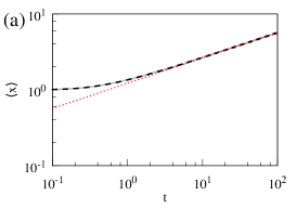
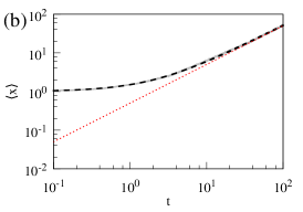
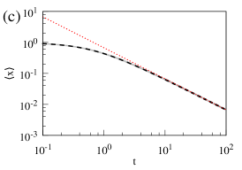
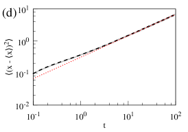
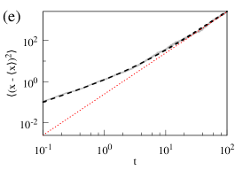
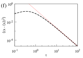
Figure 1: Dependence of the mean (a,b,c) and variance (d,e,f) on time for various values of the parameters $\eta$ and $\nu$ when the position of the diffusing particle changes according to Eq. (10). Solid gray lines show numerical result, dashed black lines are calculated using Eqs. (23) and (24), dotted (red) lines show the power-law dependence on time $\sim t^{1/[2(1-\eta)]}$ for (a,b,c) and $\sim t^{1/(1-\eta)}$ for (d,e,f). The parameters are $\sigma=1$ and $\eta=-\frac{1}{2}$, $\nu=-1$ for (a,d); $\eta=\frac{1}{2}$, $\nu=0$ for (b,c); $\eta=\frac{3}{2}$, $\nu=5$ for (c,f). The initial position is $x_{0}=1$.

We check the analytic results obtained in this Section by comparing them with numerical simulations. The power-law form of the coefficients in SDE (10) allows us to introduce an operational time $\tau$ in addition to the physical time $t$ so that the diffusion coefficient in the operational time becomes constant Ruseckas et al. (2016). The relation between the physical time $t$ and the operational time $\tau$ is specified by the equation $dt=\sigma^{-2}x^{-2\eta}d\tau$. For the numerical solution of SDE (10) we use the Euler-Maruyama scheme with a variable time step $\Delta t_{k}=\Delta\tau/(\sigma^{2}x_{k}^{2\eta})$ which is equivalent to the introduction of the operational time Ruseckas et al. (2016). Thus the numerical method of solution of SDE (10) is given by the equations

$$x_{k+1} = x_{k}+\left(\eta-\frac{\nu}{2}\right)\frac{\Delta\tau}{x_{k}}+\sqrt{\Delta\tau}\varepsilon_{k}\,,$$ (27)

$$t_{k+1} = t_{k}+\frac{\Delta\tau}{\sigma^{2}x_{k}^{2\eta}}\,.$$ (28)

Here $\Delta\tau\ll 1$ is the time step in the operational time and $\varepsilon_{k}$ are normally distributed uncorrelated random variables with a zero expectation and unit variance. To avoid the divergence of the diffusion and drift coefficients at $x=0$ in the numerical simulation, we insert a reflective boundary at $x=10^{-3}$ . This modification is analogous to the regularization of the diffusivity at $x=0$, performed in Refs. Cherstvy et al. (2013); Cherstvy and Metzler (2014). When $\eta>1$ and $\nu>1$ the PDF of $x$ increases for small values of $x$. In this case the operational time introduced in such a way that the coefficient before noise becomes proportional to the first power of $x$ can lead to a more efficient numerical method. Such an operational time is introduced by the equation $dt=\sigma^{-2}x^{-2(\eta-1)}d\tau$ and the numerical method of solution becomes

$$x_{k+1} = x_{k}\left[1+\Delta\tau\left(\eta-\frac{\nu}{2}\right)+\sqrt{\Delta\tau}\varepsilon_{k}\right]\,,$$ (29)

$$t_{k+1} = t_{k}+\frac{\Delta\tau}{\sigma^{2}x_{k}^{2(\eta-1)}}\,.$$ (30)

We have calculated the mean and the variance by averaging over $10^{5}$ trajectories. Comparison of the analytic expressions (23), (24) with numerically obtained time-dependent mean and variance is shown in Fig. 1. For numerical simulation we have chosen three different values of the exponent $\eta$: $\eta=-\frac{1}{2}$, $\eta=\frac{1}{2}$, and $\eta=\frac{3}{2}$ corresponding, respectively, to subdiffusion, superdiffusion and to the localization of the particle. For each case we have chosen a value of the parameter $\nu$ that differs from $\eta$ of the free HDP. For all numerical simulations the initial position is $x_{0}=1$. We see a good agreement of the numerical results with analytic expressions. As we can see in Fig. 1, the time dependence of the mean and the variance becomes a power-law for large times and the initial position is forgotten (for the parameters used in Fig. 1(b) and (e) the difference between the exact solution and the power-law approximation remains constant, but the relative difference is decreasing).

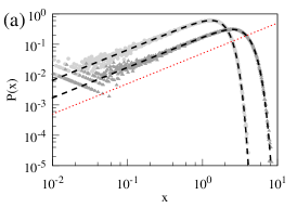
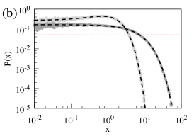
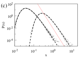
Figure 2: Time-dependent PDF $P(x,t|x_{0},0)$ corresponding to times $t=1$ (light gray) and $t=10$ (dark gray) for various values of the parameters $\eta$ and $\nu$ when the position of the diffusing particle changes according to Eq. (10). Dashed black lines are calculated using Eq. (21). The dotted line shows the slope $x^{-\nu}$. The parameters are $\sigma=1$ and (a) $\eta=-\frac{1}{2}$, $\nu=-1$; (b) $\eta=\frac{1}{2}$, $\nu=0$; (c) $\eta=\frac{3}{2}$, $\nu=5$. The initial position is $x_{0}=1$.

Comparison of the analytic expression (21) for the time-dependent PDF $P(x,t|x_{0},0)$ with the results of numerical simulation is shown in Fig. 2. To illustrate how the PDF changes with time, the PDF is shown at two different time moments $t=1$ and $t=10$. We see a good agreement of the numerical results with the analytic expression for both time moments. With increasing time the PDF shifts to the larger values of $x$ when $\eta<1$ and to the smaller values of $x$ when $\eta>1$.

IV External force leading to an exponential restriction of the diffusion

Now let us consider the external deterministic force having a power-law dependence on $x$ but with the power-law exponent different than $2\eta-1$. When such a force is positive if the power-law exponent is smaller than $2\eta-1$ and negative if the power-law exponent is larger than $2\eta-1$, the SDE describing the HDP can be written as

$$dx=\sigma^{2}\left(\left(\eta-\frac{\nu}{2}\right)x^{2\eta-1}+\frac{m_{1}}{2}x_{\mathrm{min}}^{m_{1}}x^{2\eta-1-m_{1}}-\frac{m_{2}}{2x_{\mathrm{max}}^{m_{2}}}x^{2\eta-1+m_{2}}\right)dt+\sigma x^{\eta}dW_{t}\,.$$ (31)

Here $m_{1},m_{2}>0$ and $x_{\mathrm{min}}$, $x_{\mathrm{max}}$ are the parameters of the external force. In Eq. (31) we included three terms in the drift. Each term has power-law dependence on position $x$, but with different power-law exponents: equal to $2\eta-1$, smaller than $2\eta-1$ and larger than $2\eta-1$. The steady-state PDF corresponding to Eq. (31) is

$$P_{0}(x)\sim x^{-\nu}\exp\left\{-\left(\frac{x_{\mathrm{min}}}{x}\right)^{m_{1}}-\left(\frac{x}{x_{\mathrm{max}}}\right)^{m_{2}}\right\}\,.$$ (32)

We see that the additional terms in Eq. (31) lead to exponential restriction of the diffusion. When $x_{\mathrm{min}}\ll x\ll x_{\mathrm{max}}$, the steady-state PDF has the power-law form $P_{0}(x)\sim x^{-\nu}$. Confined HDP has been investigated in Refs. Cherstvy et al. (2014b); Cherstvy and Metzler (2015). Analysis of confined HDP can be relevant for the description of the tracer particles moving in the confinement of cellular compartments or for the particle traced with optical tweezers that exert a restoring force on the particle Jeon et al. (2011).

We can mathematically obtain one of the terms in Eq. (31) leading to the exponential restriction of the diffusion by transforming the time in the initial equation. Indeed, if we start with the Itô SDE

$$dx=a(x)dt+b(x)dW_{t}$$ (33)

and introduce a new stochastic variable $z(t)=g(t)x(c(t))$ then the SDE for the stochastic variable $z$ becomes

$$dz=\left(\frac{dg(t)}{dt}\frac{z}{g(t)}+g(t)\frac{dc(t)}{dt}a\left(\frac{z}{g(t)}\right)\right)dt+g(t)\sqrt{\frac{dc(t)}{dt}}b\left(\frac{z}{g(t)}\right)dW_{t}\,.$$ (34)

In Eq. (34) a new term that is proportional to $z$ and to the derivative of $g(t)$ appears in the drift. The PDF of the stochastic variable $z$ is related to the PDF of $x$ via the equation

$$P_{z}(z,t)=\frac{1}{g(t)}P_{x}\left(\frac{z}{g(t)},c(t)\right)\,.$$ (35)

Thus, to introduce a new term into Eq. (10), let us start with a stochastic variable $y(t)$ obeying the SDE (10) and consider a new stochastic variable

$$x(t)=e^{\mu t}y\left(\frac{1}{\kappa}(e^{\kappa t}-1)\right)\,.$$ (36)

Here the functions $g(t)$ and $c(t)$ are $g(t)=e^{\mu t}$ and $c(t)=\kappa^{-1}(e^{\kappa t}-1)$. From Eq. (34) follows that the equation for the stochastic variable $x$ is

$$dx=\left(\mu x+\sigma^{2}\left(\eta-\frac{\nu}{2}\right)e^{\kappa t-2\mu(\eta-1)t}x^{2\eta-1}\right)dt+\sigma e^{\frac{1}{2}\kappa t-\mu(\eta-1)t}x^{\eta}dW_{t}\,.$$ (37)

We can obtain an equation with time-independent coefficients by requiring that

$$\kappa=2\mu(\eta-1)\,.$$ (38)

Using this value for the parameter $\kappa$ the SDE for $x$ becomes

$$dx=\left(\mu x+\sigma^{2}\left(\eta-\frac{\nu}{2}\right)x^{2\eta-1}\right)dt+\sigma x^{\eta}dW_{t}\,.$$ (39)

When $\mu$ has the same sign as $\eta-1$, this SDE can be written in the form similar to Eq. (31):

$$dx=\sigma^{2}\left(\eta-\frac{\nu}{2}+(\eta-1)\left(\frac{x_{\mathrm{m}}}{x}\right)^{2(\eta-1)}\right)x^{2\eta-1}dt+\sigma x^{\eta}dW\,,$$ (40)

where the parameter $x_{\mathrm{m}}$ is defined by the equation

$$\mu=\sigma^{2}(\eta-1)x_{\mathrm{m}}^{2(\eta-1)}\,.$$ (41)

Comparing Eq. (40) and Eq. (31) we see that the time transformation considered in this Section introduces an exponential restriction of the diffusion at small values of $x$ when $\eta>1$ and at large values of $x$ when $\eta<1$.

Using Eqs. (21) and (35) we obtain the time-dependent PDF for the stochastic variable $x$ obeying SDE (40):

$$P(x,t|x_{0},0) = \frac{2|\eta-1|x_{\mathrm{m}}^{2(\eta-1)}}{1-e^{-2\mu(\eta-1)t}}x^{\frac{1-\nu-2\eta}{2}}x_{0}^{\frac{1+\nu-2\eta}{2}}e^{\frac{1+\nu-2\eta}{2}\mu t}$$ (42)

$$\times\exp\left(-\frac{x_{\mathrm{m}}^{2(\eta-1)}}{1-e^{-2(\eta-1)\mu t}}\left(x^{2(1-\eta)}+x_{0}^{2(1-\eta)}e^{-2(\eta-1)\mu t}\right)\right)$$

$$\times I_{\frac{1+\nu-2\eta}{2(\eta-1)}}\left(\frac{x_{\mathrm{m}}^{2(\eta-1)}x^{(1-\eta)}x_{0}^{(1-\eta)}}{\sinh\left((\eta-1)\mu t\right)}\right)$$

The conditions of validity of this expression is the same as for Eq. (21). That is, the expression for the PDF given by Eq. (42) is valid when $\nu>1$ and $\eta>1$ or $\nu<1$ and $\eta<1$. The average of a power of $x$, calculated using Eq. (42), is

$$\langle x^{a}\rangle_{x_{0}} = \int_{0}^{\infty}x^{a}P(x,t|x_{0},0)dy$$ (43)

$$= \frac{\Gamma\left(\frac{\nu-1-a}{2(\eta-1)}\right)}{\Gamma\left(\frac{\nu-1}{2(\eta-1)}\right)}\frac{x_{\mathrm{m}}^{a}}{(1-e^{-2(\eta-1)\mu t})^{\frac{a}{2(\eta-1)}}}\,{}_{1}F_{1}\left(\frac{a}{2(\eta-1)};\frac{\nu-1}{2(\eta-1)};-\frac{x_{\mathrm{m}}^{2(\eta-1)}x_{0}^{2(1-\eta)}}{e^{2(\eta-1)\mu t}-1}\right)\,.$$

This average is finite under the same conditions as Eq. (22). In particular, the average of $x$ is equal to

$$\langle x\rangle_{x_{0}}=\frac{\Gamma\left(\frac{\nu-2}{2(\eta-1)}\right)}{\Gamma\left(\frac{\nu-1}{2(\eta-1)}\right)}\frac{x_{\mathrm{m}}}{(1-e^{-2(\eta-1)\mu t})^{\frac{1}{2(\eta-1)}}}\,{}_{1}F_{1}\left(\frac{1}{2(\eta-1)};\frac{\nu-1}{2(\eta-1)};-\frac{x_{\mathrm{m}}^{2(\eta-1)}x_{0}^{2(1-\eta)}}{e^{2(\eta-1)\mu t}-1}\right)$$ (44)

and is finite when $\nu>2$ and $\eta>1$ or $\nu<1$ and $\eta<1$. The average of the square of $x$ is equal to

$$\langle x^{2}\rangle_{x_{0}}=\frac{\Gamma\left(\frac{\nu-3}{2(\eta-1)}\right)}{\Gamma\left(\frac{\nu-1}{2(\eta-1)}\right)}\frac{x_{\mathrm{m}}^{2}}{(1-e^{-2(\eta-1)\mu t})^{\frac{1}{\eta-1}}}\,{}_{1}F_{1}\left(\frac{1}{(\eta-1)};\frac{\nu-1}{2(\eta-1)};-\frac{x_{\mathrm{m}}^{2(\eta-1)}x_{0}^{2(1-\eta)}}{e^{2(\eta-1)\mu t}-1}\right)$$ (45)

and is finite when $\nu>3$ and $\eta>1$ or $\nu<1$ and $\eta<1$.

When $\mu$ has the same sign as $\eta-1$ and $t\rightarrow\infty$ then the PDF (42) tends to the steady-state PDF

$$P_{0}(x)=\frac{2|\eta-1|x_{\mathrm{m}}^{\nu-1}}{\Gamma\left(\frac{\nu-1}{2(\eta-1)}\right)}x^{-\nu}\exp\left(-\left(\frac{x_{\mathrm{m}}}{x}\right)^{2(\eta-1)}\right)\,.$$ (46)

The steady-state PDF (46) leads to the steady-state averages of $x$ and $x^{2}$

$$\langle x\rangle_{\mathrm{st}} = \frac{\Gamma\left(\frac{\nu-2}{2(\eta-1)}\right)}{\Gamma\left(\frac{\nu-1}{2(\eta-1)}\right)}x_{\mathrm{m}}\,,$$ (47)

$$\langle x^{2}\rangle_{\mathrm{st}} = \frac{\Gamma\left(\frac{\nu-3}{2(\eta-1)}\right)}{\Gamma\left(\frac{\nu-1}{2(\eta-1)}\right)}x_{\mathrm{m}}^{2}\,.$$ (48)

Now let us consider the time evolution of the average $\langle x^{2}\rangle_{x_{0}}$, given by Eq. (45). In the case when the initial position $x_{0}$ is far from the cut-off boundary $x_{\mathrm{m}}$ (that is $x_{0}\ll x_{\mathrm{m}}$ when $\eta<1$ and $x_{0}\gg x_{\mathrm{m}}$ when $\eta>1$), the time evolution of the average $\langle x^{2}\rangle_{x_{0}}$ can be separated into three parts. First, for small times

$$t\ll\frac{x_{0}^{2(1-\eta)}}{2(\eta-1)^{2}\sigma^{2}}$$

the influence of the initial position is significant and the diffusion is approximately normal, $\langle x^{2}\rangle_{x_{0}}$ depends linearly on time $t$. For the intermediate times

$$\frac{x_{0}^{2(1-\eta)}}{2(\eta-1)^{2}\sigma^{2}}\ll t\ll\frac{1}{2(\eta-1)\mu}=\frac{x_{\mathrm{m}}^{2(1-\eta)}}{2(\eta-1)^{2}\sigma^{2}}$$

the exponent $e^{-2(\eta-1)\mu t}$ in Eq. (45) differs from $1$ only slightly, however the last argument of the hypergeometric function is already small. Approximating the hypergeometric function by $1$ and expanding the exponent $e^{-2(\eta-1)\mu t}$ into power series and keeping only the linear term we obtain that the average $\langle x^{2}\rangle_{x_{0}}$ depends on time as a power-law, $\langle x^{2}\rangle_{x_{0}}\sim t^{1/(1-\eta)}$. Thus for this intermediate range of time the anomalous diffusion occurs. Finally, for large times

$$t\apprge\frac{1}{2(\eta-1)\mu}$$

the cut-off position $x_{\mathrm{m}}$ starts to influence the diffusion and $\langle x^{2}\rangle_{x_{0}}$ approaches the steady-state value (48). We can conclude that the introduction of the boundary via an exponential cut-off does not change the anomalous diffusion when the starting position is far from the boundary ant the time is not too large.

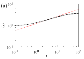
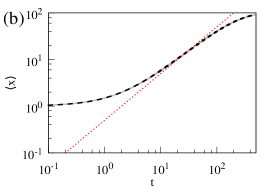
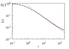
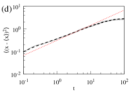
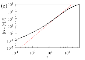
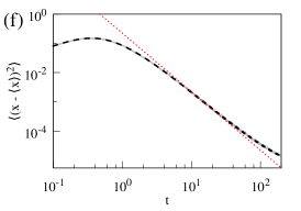
Figure 3: Dependence of the mean (a,b,c) and variance (d,e,f) on time for various values of the parameters $\eta$ and $\nu$ when the position of the diffusing particle changes according to Eq. (40). Solid gray lines show numerical result, dashed black lines are calculated using Eqs. (44) and (45), dotted (red) lines show the power-law dependence on time $\sim t^{1/[2(1-\eta)]}$ for (a,b,c) and $\sim t^{1/(1-\eta)}$ for (d,e,f). The parameters are $\sigma=1$ and $\eta=-\frac{1}{2}$, $\nu=-1$, $x_{\mathrm{m}}=5$ for (a,d); $\eta=\frac{1}{2}$, $\nu=0$, $x_{\mathrm{m}}=100$ for (b,c); $\eta=\frac{3}{2}$, $\nu=5$ $x_{\mathrm{m}}=0.01$ for (c,f). The initial position is $x_{0}=1$.

Comparison of the analytic expressions (44), (45) with numerically obtained time-dependent mean and variance is shown in Fig. 3. As in Sec. III, for numerical solution we use the Euler-Maruyama scheme with a variable time step, equivalent to the introduction of the operational time in addition to the physical time $t$. When the diffusion coefficient in the operational time $\tau$ does not depend on position $x$, the numerical method is given by the equations

$$x_{k+1} = x_{k}+\left[\left(\eta-\frac{\nu}{2}\right)\frac{1}{x_{k}}+(\eta-1)x_{\mathrm{m}}^{2(\eta-1)}x_{k}^{1-2\eta}\right]\Delta\tau+\sqrt{\Delta\tau}\varepsilon_{k}\,,$$ (49)

$$t_{k+1} = t_{k}+\frac{\Delta\tau}{\sigma^{2}x_{k}^{2\eta}}\,.$$ (50)

When $\eta>1$, a more efficient numerical method is obtained when the change of the variable $x$ in one step is proportional to the value of the variable. Then the numerical method of solution is described by the equations

$$x_{k+1} = x_{k}\left[1+\Delta\tau\left(\eta-\frac{\nu}{2}\right)+\Delta\tau(\eta-1)\left(\frac{x_{\mathrm{m}}}{x_{k}}\right)^{2(\eta-1)}+\sqrt{\Delta\tau}\varepsilon_{k}\right]\,,$$ (51)

$$t_{k+1} = t_{k}+\frac{\Delta\tau}{\sigma^{2}x_{k}^{2(\eta-1)}}\,.$$ (52)

When $\eta<1$, to avoid the divergence of the diffusion and drift coefficients at $x=0$ in the numerical simulation, we insert a reflective boundary at $x=10^{-3}$ . This is not necessary when $\eta>1$ because the additional term in the drift creates an exponential cut-off at small values of $x\sim x_{\mathrm{m}}$. For numerical simulation we used the same values of the parameters $\eta$ and $\nu$ as in Fig. 1, the initial position is $x_{0}=1$. We have chosen the parameter $x_{\mathrm{m}}$ of the external force so that the initial position $x_{0}$ is far from the boundary $x_{\mathrm{m}}$. In Fig. 3 we see a good agreement of the numerical results with analytic expressions. The numerical calculation and the analytic expressions confirm the presence of a time interval where the mean and the variance have a power-law dependence on time, as can be seen in Fig. 3. The upper limit of this time interval is determined by the the position $x_{\mathrm{m}}$ of the exponential cut-off.

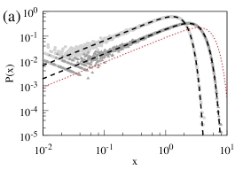
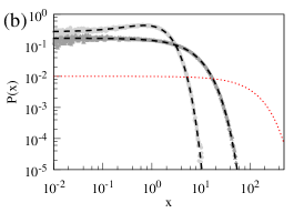
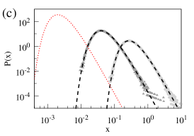
Figure 4: Time-dependent PDF $P(x,t|x_{0},0)$ corresponding to times $t=1$ (light gray) and $t=10$ (dark gray) for various values of the parameters $\eta$ and $\nu$ when the position of the diffusing particle changes according to Eq. (40). Dashed black lines are calculated using Eq. (42). The dotted line shows the steady-state PDF (46). The parameters are $\sigma=1$ and (a) $\eta=-\frac{1}{2}$, $\nu=-1$, $x_{\mathrm{m}}=5$; (b) $\eta=\frac{1}{2}$, $\nu=0$, $x_{\mathrm{m}}=100$; (c) $\eta=\frac{3}{2}$, $\nu=5$ $x_{\mathrm{m}}=0.01$. The initial position is $x_{0}=1$.

Comparison of the analytic expression (42) for the time-dependent PDF $P(x,t|x_{0},0)$ with the results of numerical simulation is shown in Fig. 4. We see a good agreement of the numerical results with the analytic expression. With increasing time the PDF shifts to the larger values of $x$ when $\eta<1$ and to the smaller values of $x$ when $\eta>1$. However, in contrast to the situation in the previous Section where the restricting force was not present, this shift of the PDF now is limited, at large times the time-depend PDF approaches the steady-state PDF (46).

V Conclusions

In summary, we have obtained analytic expressions (21) and (42) for the transition probability of the heterogeneous diffusion process whose diffusivity has a power-law dependence on the distance $x$. In the description of the HDP we have included an additional deterministic force that also has a power-law dependence on the position. The drift term having a power-law dependence on the position can arise not only due to an external force but can also represent a noise-induced drift Volpe and Wehr (2016). Such a drift term appears in a Langevin equation describing overdamped fluctuations of the position of a particle in nonhomogeneous medium Sancho et al. (1982). Stochastic differential equations with power-law drift and diffusion terms have been used to model random fluctuations of the atmospheric forcing on the ocean circulation Ditlevsen (1999) and pressure time series routinely used to define the index characterizing the North Atlantic Oscillation Lind et al. (2005). The Brownian motion of a colloidal particle in water subjected to the gravitational force and with a space-dependent diffusivity due to the presence of the bottom wall of the sample cell has been investigated in Ref. Volpe et al. (2010). Force causing exponential cut-off in the PDF of the particle position can describe HDP process in confined regions; such a description can be relevant, for example, for the tracer particles moving in the confinement of cellular compartments Jeon et al. (2011); Kühn et al. (2011).

A system obeying SDEs with power-law drift and diffusion terms can be experimetally realized as an electrical circuit driven by a multiplicative noise, similarly as in Ref. Smythe et al. (1983). The equation describing the overdamped motion of the Brownian particle takes the form of Eq. (10) when a temperature gradient is present in the medium and the particle is subjected to the external potential that is proportional to the temperature profile Kazakevičius and Ruseckas (2015). In particular, steady state heat transfer due to the temperature difference between the beginning and the end of the system corresponds to $\eta=1/2$ in Eq. (10) Kazakevičius and Ruseckas (2015). For a charged particle the external force can be introduced by applying the electric potential difference at the ends of the system.

When the power-law exponent in the deterministic force is equal to $2\eta-1$, where $2\eta$ is the power-law exponent in the dependence of the diffusion coefficient on the position, the external force does not limit the region of diffusion. Other values of the power-law exponent in the deterministic force can cause the exponential cut-off in the PDF of the particle positions. Such an exponential restriction of the diffusion appears when the external force is positive if the power-law exponent is smaller than $2\eta-1$ and negative if the power-law exponent is larger than $2\eta-1$. We obtained an analytic expression (42) for the transition probability in a particular case when the external restricting force has a linear dependence on the position. Using analytic expression for the transition probability we calculated the time dependence of the moments of the particle position, Eqs. (22) and (43).

We found that the power-law exponent in the dependence of the MSD on time does not depend on the external force, this force changes only the anomalous diffusion coefficient. This conclusion is valid for sufficiently large times satisfying the condition (25), that is when the initial position of the particle is forgotten and the anomalous diffusion occurs. In addition, the external force having the power-law exponent different from $2\eta-1$ limits the time interval where the anomalous diffusion occurs. The conclusions remain valid also when the external force can be represented as a sum of several terms, each term being a power-law function of position with a different power-law exponent. Thus, our results indicate that the anomalous diffusion caused by diffusivity being a power-law function of the position is robust with respect to an external perturbation, the exponent $\alpha$ in Eq. (1) is determined only by the diffusion coefficient.

In addition, the results of Sec. III show that the character of the anomalous diffusion does not depend on the interpretation of the Langevin equation: the scaling exponent $\alpha$ in Eq. (1) is the same for both Stratonovich and Itô conventions. This is because different interpretations correspond to the different values of the parameter $\nu$ in Eq. (10): Stratonovich convention results in $\nu=\eta$, Itô convention in $\nu=2\eta$, and the scaling exponent $\alpha$ does not depend on $\nu$. The same conclusion that the exponent of the anomalous diffusion does not depend on the prescription has been obtained in Refs. Fa and Lenzi (2003); Fa (2005); Heidernätsch (2015) for equations describing diffusion without the presence of an external force.

Appendix A Solution of the Fokker-Planck equation for the Bessel process

Let us consider the Fokker-Planck equation

$$\frac{\partial}{\partial t}P=\frac{\nu}{2}\frac{\partial}{\partial x}\frac{1}{x}P+\frac{1}{2}\frac{\partial^{2}}{\partial x^{2}}P$$ (53)

and search for the time-dependent solution $P(x,t|x_{0},0)$ with the initial condition $P(x,0|x_{0},0)=\delta(x-x_{0})$. The unnormalized time-independent solution of Eq. (53) is $x^{-\nu}$. The boundary condition at $x=0$ for Eq. (53) can be expressed using the probability current Risken (1989)

$$S(x,t)=-\frac{\nu}{2x}P(x,t)-\frac{1}{2}\frac{\partial}{\partial x}P(x,t)\,.$$ (54)

We consider the boundary condition corresponding to the vanishing probability current at $x=0$, $S(0,t)=0$.

One of the possible ways to obtain the solution of Eq. (53) is to use a Laplace transform Jeanblanc et al. (2009). Here we solve Eq. (53) using the method of eigenfunctions. This method has been used in Ref. Ruseckas and Kaulakys (2010) for an equation, similar to Eq. (53). An ansatz of the form

$$P(x,t)=P_{\lambda}(x)e^{-\lambda t}$$ (55)

leads to the equation

$$\frac{\nu}{2}\frac{\partial}{\partial x}\frac{1}{x}P_{\lambda}+\frac{1}{2}\frac{\partial^{2}}{\partial x^{2}}P_{\lambda}=-\lambda P_{\lambda}\,,$$ (56)

where $P_{\lambda}(x)$ are the eigenfunctions and $\lambda\geqslant 0$ are the corresponding eigenvalues. The eigenfunctions obey the orthonormality relation Risken (1989)

$$\int_{0}^{\infty}x^{\nu}P_{\lambda}(x)P_{\lambda^{\prime}}(x)\,dx=\delta(\lambda-\lambda^{\prime})\,.$$ (57)

Expansion of the transition probability density $P(x,t|x_{0},0)$ in terms of the eigenfunctions has the form Risken (1989)

$$P(x,t|x_{0},0)=\int_{0}^{\infty}P_{\lambda}(x)x_{0}^{\nu}P_{\lambda}(x_{0})e^{-\lambda t}d\lambda\,.$$ (58)

For the solution of Eq. (56) it is convenient to write the eigenfunctions $P_{\lambda}(x)$ as

$$P_{\lambda}(x)=x^{1-\gamma}u_{\lambda}(x)\,,$$ (59)

where

$$\gamma=\frac{1+\nu}{2}\,.$$ (60)

Similar anzatz has been used in Refs. Bray (2000); Martin et al. (2011). The functions $u_{\lambda}(x)$ obey the equation

$$x^{2}\frac{d^{2}}{dx^{2}}u_{\lambda}+x\frac{d}{dx}u_{\lambda}+(\rho^{2}x^{2}-\gamma^{2})u_{\lambda}=0\,,$$ (61)

where

$$\rho=\sqrt{2\lambda}\,.$$ (62)

The probability current $S_{\lambda}(x)$, Eq. (54), rewritten in terms of functions $u_{\lambda}$, becomes

$$S_{\lambda}(x)=-\frac{1}{2}x^{-\gamma}\left(\gamma u_{\lambda}(x)+x\frac{d}{dx}u_{\lambda}(x)\right)\,.$$ (63)

The orthonormality of eigenfunctions (57) yields the orthonormality for functions $u_{\lambda}(x)$

$$\int_{0}^{\infty}xu_{\lambda}(x)u_{\lambda^{\prime}}(x)\,dx=\delta(\lambda-\lambda^{\prime})\,.$$ (64)

The general solution of Eq. (61) is

$$u_{\lambda}(x)=c_{1}J_{\gamma}(\rho x)+c_{2}Y_{\gamma}(\rho x)\,,$$ (65)

where $J_{\gamma}(x)$ and $Y_{\gamma}(x)$ are the Bessel functions of the first and second kind, respectively. The coefficients $c_{1}$ and $c_{2}$ needs to be determined from the boundary and normalization conditions for the functions $u_{\lambda}(x)$. Using Eqs. (65) and (63) we get the probability current

$$S_{\lambda}(x)=-\frac{1}{2}\rho x^{1-\gamma}[c_{1}J_{\gamma-1}(\rho x)+c_{2}Y_{\gamma-1}(\rho x)]\,.$$ (66)

The requirement $S_{\lambda}(0)=0$ leads to the condition $c_{2}=-c_{1}\tan(\pi\gamma)$. Taking into account this relation between $c_{2}$ and $c_{1}$ we obtain

$$u_{\lambda}(x)=c_{\lambda}J_{-\gamma}(\rho x)\,.$$ (67)

In addition, the condition $S_{\lambda}(0)=0$ implies $c_{2}=0$ when $\gamma\geqslant 1$. Thus, when $\gamma\geqslant 1$, $\nu\geqslant 1$ both coefficients $c_{1}$ and $c_{2}$ are zero and the solution (58) is not valid. It is known that for a Bessel process with such parameters a total absorption at the origin occurs in a finite time Karlin and Taylor (1981).

Orthonormality condition (64) leads to the equation

$$c_{\lambda}c_{\lambda^{\prime}}\int_{0}^{\infty}xJ_{-\gamma}(\rho x)J_{-\gamma}(\rho^{\prime}x)\,dx=\delta(\lambda-\lambda^{\prime})\,.$$ (68)

Since for the Bessel functions the equality

$$\rho\int_{0}^{\infty}xJ_{\gamma}(\rho x)J_{\gamma}(\rho^{\prime}x)xdx=\delta(\rho-\rho^{\prime})$$ (69)

is valid, we obtain $c_{\lambda}=1$. Using Eqs. (58), (59) and (67) the solution of the Fokker-Planck equation can be expressed as

$$P(x,t|x_{0},0)=x^{1-\gamma}x_{0}^{\gamma}\int_{0}^{\infty}J_{-\gamma}(\rho x)J_{-\gamma}(\rho x_{0})e^{-\frac{1}{2}\rho^{2}t}\rho d\rho\,.$$ (70)

Integration yields

$$P(x,t|x_{0},0)=\frac{x^{1-\gamma}x_{0}^{\gamma}}{t}\exp\left(-\frac{x^{2}+x_{0}^{2}}{2t}\right)I_{-\gamma}\left(\frac{xx_{0}}{t}\right)\,.$$ (71)

Here $I_{\alpha}(x)$ is the modified Bessel function of the first kind.

References

- Bouchaud and Georges (1990) J.-P. Bouchaud and A. Georges, Phys. Rep. 195, 127 (1990).
- Evers et al. (2013) F. Evers, C. Zunke, R. D. L. Hanes, J. Bewerunge, I. Ladadwa, A. Heuer, and S. U. Egelhaaf, Phys. Rev. E 88, 022125 (2013).
- Chepizhko and Peruani (2013) O. Chepizhko and F. Peruani, Phys. Rev. Lett. 111, 160604 (2013).
- Metzler and Klafter (2000) R. Metzler and J. Klafter, Phys. Rep. 339, 1 (2000).
- Schubert et al. (2013) M. Schubert, E. Preis, J. C. Blakesley, P. Pingel, U. Scherf, and D. Neher, Phys. Rev. B 87, 024203 (2013).
- Scalliet et al. (2015) C. Scalliet, A. Gnoli, A. Puglisi, and A. Vulpiani, Phys. Rev. Lett 114, 198001 (2015).
- Fogedby (1994) H. C. Fogedby, Phys. Rev. Lett. 73, 2517 (1994).
- Marandet et al. (2003) Y. Marandet, H. Capes, L. Godbert-Mouret, R. Guirlet, M. Koubiti, and R. Stamm, Commun. Nonlinear. Sci. Commun. 8, 469 (2003).
- Mercadier et al. (2009) N. Mercadier, W. Guerin, M. Chevrollier, and R. Kaiser, Nat. Phys. 5, 602 (2009).
- Tabei et al. (2013) S. M. A. Tabei, S. Burov, H. Y. Kim, A. Kuznetsov, T. Huynh, J. Jureller, L. H. Philipson, A. R. Dinner, and N. F. Scherer, Proc. Natl Acad. Sci. USA 110, 4911 (2013).
- Weigel et al. (2011) A. V. Weigel, B. Simon, M. M. Tamkun, and D. Krapf, Proc. Natl Acad. Sci. USA 108, 6438 (2011).
- Jeon et al. (2011) J.-H. Jeon, V. Tejedor, S. Burov, E. Barkai, C. Selhuber-Unkel, K. Berg-Sørensen, L. Oddershede, and R. Metzler, Phys. Rev. Lett. 106, 048103 (2011).
- Wong et al. (2004) I. Y. Wong, M. L. Gardel, D. R. Reichman, E. R. Weeks, M. T. Valentine, A. R. Bausch, and D. A. Weitz, Phys. Rev. Lett. 92, 178101 (2004).
- Scher and Montroll (1975) H. Scher and E. W. Montroll, Phys. Rev. B 12, 2455 (1975).
- Jeon et al. (2012) J.-H. Jeon, H. Martinez-Seara Monne, M. Javanainen, and R. Metzler, Phys. Rev. Lett. 109, 188103 (2012).
- Kneller et al. (2011) G. R. Kneller, K. Baczynski, and M. Pasienkewicz-Gierula, J. Chem. Phys 135, 141105 (2011).
- Kepten et al. (2013) E. Kepten, I. Bronshtein, and Y. Garini, Phys. Rev. E 87, 052713 (2013).
- Szymanski and Weiss (2009) J. Szymanski and M. Weiss, Phys. Rev. Lett. 103, 038102 (2009).
- Jeon et al. (2013) J.-H. Jeon, N. Leijnse, L. B. Oddershede, and R. Metzler, New J. Phys. 15, 045011 (2013).
- Kühn et al. (2011) T. Kühn, T. O. Ihalainen, J. Hyväluoma, N. Dross, S. F. Willman, J. Langowski, M. Vihinen-Ranta, and J. Timonen, PLoS ONE 6, e22962 (2011).
- Cherstvy et al. (2013) A. G. Cherstvy, A. V. Chechkin, and R. Metzler, New J. Phys. 15, 083039 (2013).
- Cherstvy and Metzler (2013) A. G. Cherstvy and R. Metzler, Phys. Chem. Chem. Phys 15, 20220 (2013).
- Cherstvy et al. (2014a) A. G. Cherstvy, A. V. Chechkin, and R. Metzler, Soft Matter 10, 1591 (2014a).
- Cherstvy and Metzler (2014) A. G. Cherstvy and R. Metzler, Phys. Rev. E 90, 012134 (2014).
- Maeda et al. (2012) Y. T. Maeda, T. Tlusty, and A. Libchaber, Proc. Natl. Acad. Sci. 109, 17972 (2012).
- Mast et al. (2013) C. B. Mast, S. Schink, U. Gerland, and D. Braun, Proc. Natl. Acad. Sci. 110, 8030 (2013).
- Haggerty and Gorelick (1995) R. Haggerty and S. M. Gorelick, Water Resources Res. 31, 2383 (1995).
- Dentz and Bolster (2010) M. Dentz and D. Bolster, Phys. Rev. Lett. 105, 244301 (2010).
- Richardson (1926) L. F. Richardson, Proc. R. Soc. Lond. A 110, 709 (1926).
- O’Shaughnessy and Procaccia (1985) B. O’Shaughnessy and I. Procaccia, Phys. Rev. Lett. 54, 455 (1985).
- Loverdo et al. (2009) C. Loverdo, O. Bénichou, R. Voituriez, A. Biebricher, I. Bonnet, and P. Desbiolles, Phys. Rev. Lett. 102, 188101 (2009).
- English et al. (2011) B. P. English, V. Hauryliuk, A. Sanamrad, S. Tankov, N. H. Dekker, and J. Elf, Proc. Natl Acad. Sci. USA 108, E365 (2011).
- Kazakevičius and Ruseckas (2015) R. Kazakevičius and J. Ruseckas, J. Stat. Mech. 2015, P02021 (2015).
- Srokowski (2014) T. Srokowski, Phys. Rev. E 89, 030102(R) (2014).
- Schertzer et al. (2001) D. Schertzer, M. Larchevêque, J. Duan, V. V. Yanovsky, and S. Lovejoy, J. Math. Phys. 42, 200 (2001).
- Dentz et al. (2012) M. Dentz, P. Gouze, A. Russian, J. Dweik, and F. Delay, Adv. Water Res. 49, 13 (2012).
- Cohen (2005) A. E. Cohen, Phys. Rev. Lett. 94, 118102 (2005).
- Manning (1969) G. S. Manning, J. Chem. Phys. 51, 924 (1969).
- Sagi et al. (2012) Y. Sagi, M. Brook, I. Almog, and N. Davidson, Phys. Rev. Lett. 108, 093002 (2012).
- Bouchet and Dauxois (2005) F. Bouchet and T. Dauxois, Phys. Rev. E 72, 045103(R) (2005).
- Wu et al. (2009) L. A. Wu, S. S. Wu, and D. Segal, Phys. Rev. E 79, 061901 (2009).
- Gardiner (2004) C. W. Gardiner, Handbook of Stochastic Methods for Physics, Chemistry and the Natural Sciences (Springer-Verlag, Berlin, 2004).
- Lau and Lubensky (2007) A. W. C. Lau and T. C. Lubensky, Phys. Rev. E 76, 011123 (2007).
- Fuliński (2011) A. Fuliński, Phys. Rev. E 83, 061140 (2011).
- Volpe and Wehr (2016) G. Volpe and J. Wehr, Rep. Prog. Phys. 79, 053901 (2016).
- Kaulakys and Ruseckas (2004) B. Kaulakys and J. Ruseckas, Phys. Rev. E 70, 020101(R) (2004).
- Kaulakys et al. (2006) B. Kaulakys, J. Ruseckas, V. Gontis, and M. Alaburda, Physica A 365, 217 (2006).
- Gontis et al. (2010) V. Gontis, J. Ruseckas, and A. Kononovicius, Physica A 389, 100 (2010).
- Mathiesen et al. (2013) J. Mathiesen, L. Angheluta, P. T. H. Ahlgren, and M. H. Jensen, Proc. Natl. Acad. Sci. 110, 17259 (2013).
- Ton and Daffertshofer (2016) R. Ton and A. Daffertshofer, NeuroImage (2016), doi: 10.1016/j.neuroimage.2016.01.008.
- Karatzas and Shreve (2012) I. Karatzas and S. Shreve, Brownian Motion and Stochastic Calculus (Springer, New York, 2012).
- Hänggi and Thomas (1982) P. Hänggi and H. Thomas, Phys. Rep. 88, 207 (1982).
- Klimontovich (1994) Y. L. Klimontovich, Phys. Usp. 37, 737 (1994).
- Pesce et al. (2013) G. Pesce, A. McDaniel, S. Hottovy, J. Wehr, and G. Volpe, Nat. Commun. 4, 2733 (2013).
- dos Santos and Tsallis (2010) B. C. dos Santos and C. Tsallis, Phys. Rev. E 82, 061119 (2010).
- Sokolov (2010) I. M. Sokolov, Chem. Phys. 375, 359 (2010).
- van Kampen (1981) N. G. van Kampen, J. Stat. Phys. 24, 175 (1981).
- Heidernätsch (2015) M. Heidernätsch, On the diffusion in inhomogeneous systems, Ph.D. thesis, Technische Universität Chemnitz, Faculty of Sciences, Institute of Physics, Complex Systems and Nonlinear Dynamics (2015).
- Kwok (2012) S. F. Kwok, Ann. Phys. 327, 1989 (2012).
- Arenas et al. (2014) Z. G. Arenas, D. G. Barci, and C. Tsallis, Phys. Rev. E 90, 032118 (2014).
- Jeanblanc et al. (2009) M. Jeanblanc, M. Yor, and M. Chesney, Mathematical Methods for Financial Markets (Springer, London, 2009).
- Bray (2000) A. J. Bray, Phys. Rev. E 62, 103 (2000).
- Martin et al. (2011) E. Martin, U. Behn, and G. Germano, Phys. Rev. E 83, 051115 (2011).
- Karlin and Taylor (1981) S. Karlin and H. M. Taylor, A Second Course in Stochastic Processes, 2nd ed. (Academic, New York, 1981).
- Ruseckas et al. (2016) J. Ruseckas, R. Kazakevicius, and B. Kaulakys, J. Stat. Mech. 2016, 054022 (2016).
- Cherstvy et al. (2014b) A. G. Cherstvy, A. V. Chechkin, and R. Metzler, J. Phys. A: Math. Theor. 47, 485002 (2014b).
- Cherstvy and Metzler (2015) A. G. Cherstvy and R. Metzler, J. Stat. Mech. 2015, P05010 (2015).
- Sancho et al. (1982) J. M. Sancho, M. San Miguel, and D. Dürr, J. Stat. Phys. , 291 (1982).
- Ditlevsen (1999) P. D. Ditlevsen, Geophys. Res. Lett. 26, 1441 (1999).
- Lind et al. (2005) P. G. Lind, A. Mora, J. A. C. Gallas, and M. Haase, Phys. Rev. E 72, 056706 (2005).
- Volpe et al. (2010) G. Volpe, L. Helden, T. Brettschneider, J. Wehr, and C. Bechinger, Phys. Rev. Lett. 104, 170602 (2010).
- Smythe et al. (1983) J. Smythe, F. Moss, and P. V. E. McClintock, Phys. Rev. Lett. 51, 1062 (1983).
- Fa and Lenzi (2003) K. S. Fa and E. K. Lenzi, Phys. Rev. E 67, 061105 (2003).
- Fa (2005) K. S. Fa, Phys. Rev. E 72, 020101 (2005).
- Risken (1989) H. Risken, The Fokker-Planck Equation: Methods of Solution and Applications (Springer-Verlag, Berlin, 1989).
- Ruseckas and Kaulakys (2010) J. Ruseckas and B. Kaulakys, Phys. Rev. E 81, 031105 (2010).