Pion transition form factor through Dyson-Schwinger equations

Abstract

In the framework of Dyson-Schwinger equations (DSE), we compute the $\gamma^{*}\gamma\to\pi^{0}$ transition form factor, $G(Q^{2})$. For the first time, in a continuum approach to quantun chromodynamics (QCD), it was possible to compute $G(Q^{2})$ on the whole domain of space-like momenta. Our result agrees with CELLO, CLEO and Belle collaborations and, with the well-known asymptotic QCD limit, $2f_{\pi}$. Our analysis unifies this prediction with that of the pion’s valence-quark parton distribution amplitude (PDA) and elastic electromagnetic form factor.

1 Introduction

The neutral pion transition form factor is measured through electron-positron scattering. Although the available data of CELLO [1], CLEO [2], Babar [3] and Belle [4] collaborations agree in the domain of $Q^{2}<10$ GeV², the Babar and Belle data (the only data available above that point) are notoriously different. Moreover, how possibly the Babar data can reconcile with the asymptotic QCD limit, calculated by Brodsky and Lepage in [5], i.e., $2f_{\pi}$, remains unclear and unsatisfactory.

We have previous DSE input from [6], but because of the numerical methods developed by that time, it was not possible to arrive at momentum scales larger than $Q^{2}>4$ GeV². Complete understanding of $G(Q^{2})$ demands simultaneously achieving correct asymptotic behavior, but also the essentially non perturbative Abelian anomaly, $2f_{\pi}G(Q^{2}=0)=1$. Such features are achievable in the framework of DSEs. At the same time, we are able to connect our results with that of the pion’s PDA, [7], and elastic electromagnetic form factor, [8]. The reference to our detailed published article is [9]. Most of the ingredients which have gone into this study are quite general and can be applied to other mesons and processes. In particular, the study of $\gamma^{*}\gamma\to\eta_{c}$ and $\gamma^{*}\gamma\to\eta_{b}$ is under way.

2 The tools

For any pseudoscalar meson ($PS$), the $\gamma^{*}\gamma\to PS$ is expressed through $\mathcal{T}_{\mu\nu}(k_{1},k_{2})=T_{\mu\nu}(k_{1},k_{2})+T_{\mu\nu}(k_{2},k_{1})$, where the matrix element is:

$$T_{\mu\nu}(k_{1},k_{2})=\frac{e^{2}}{4\pi^{2}}\epsilon_{\mu\nu\alpha\beta}k_{1\alpha}k_{2\beta}\;G(k_{1}^{2},k_{2}^{2},k_{1}\cdot k_{2})\;.$$ (1)

The photons’ momenta are $k_{1}$ and $k_{2}$ and the meson’s total momentum is $P=k_{1}+k_{2}$ ($P^{2}=-m_{PS}^{2}$). At leading order (rainbow-ladder truncation) in the systematic and symmetry preserving DSE truncation scheme, one can write:

$$T_{\mu\nu}(k_{1},k_{2})=\int\frac{d^{4}k}{(2\pi)^{4}}i\mathcal{Q}\chi_{\mu}(l,l_{1})\Gamma_{PS}(l_{1},l_{2})S(l_{2})i\mathcal{Q}\Gamma_{\nu}(l_{2},l)\;.$$ (2)

Here $\mathcal{Q}$ is the quark charge operator ($e\;\mbox{diag}[2/3,-1/3]$ for neutral pion), $l_{1}=l+k_{1}$, $l_{2}=l-k_{2}$, where the kinematic constraints are: $k_{1}^{2}=Q^{2}$, $k_{2}^{2}=0$, $k_{1}\cdot k_{2}=-(m_{PS}^{2}+Q^{2})/2$ and $P^{2}=-m_{PS}^{2}$. The quark propagator, $S(k)$, and the Bethe-Salpeter amplitude (BSA), $\Gamma_{PS}(q_{1},q_{2})$, are obtained by solving the corresponding DSEs and the BSEs. On the other hand, the quark-photon vertex is constructed via the gauge technique, [10]. We give the details in the following subsections.

2.1 Quark propagator and Bethe-Salpeter amplitudes

Most generally, the quark propagator is written as $S(p)=-i\gamma\cdot p\sigma_{v}(p^{2})+\sigma_{s}(p^{2})$, while the BSA is:

$$\Gamma_{PS}(k;P)=\gamma_{5}[i\;E_{PS}(k;P)+\gamma\cdot PF_{PS}(k;P)+\gamma\cdot k\;k\cdot PG_{PS}(k;P)+\sigma_{\mu\nu}k_{\mu}P_{\nu}H_{PS}(k;P)]\;,$$ (3)

The corresponding DSE and BSE, in the rainbow-ladder truncation, are:

$$S^{-1}(p) = \mathcal{Z}_{2F}(S^{0})^{-1}(p)+\mathcal{Z}_{1F}\int\frac{d^{4}q}{(2\pi)^{4}}G(p-q)D_{\mu\nu}^{0}(p-q,\mu)\frac{\lambda^{a}}{2}\gamma_{\mu}S(q,\mu)\frac{\lambda^{a}}{2}\gamma_{\nu},$$ (4)

$$\Gamma_{PS}(p,P) = -\int\frac{d^{4}q}{(2\pi)^{4}}\frac{G((p-q)^{2})}{(p-q)^{2}}\frac{\lambda^{c}}{2}\gamma_{\mu}S^{a}(q+\eta P)\Gamma_{PS}(q,P)S^{b}(q-(1-\eta P))\frac{\lambda^{c}}{2}\gamma_{\nu}\;,$$ (5)

with $G(p-q)$ being the effective coupling described in [11]. Once we obtain the solution of Eq. (4), we can parameterize it in the form of a complex conjugate pole representation:

$$S(p)=\sum_{j=1}^{N}\left(\frac{z_{j}}{i\gamma\cdot p+m_{j}}+\frac{z_{j}^{*}}{i\gamma\cdot p+m_{j}^{*}}\right)\;,$$ (6)

constrained to the ultraviolet conditions of free quark propagator; $N=2$ is accurate enough for our purposes. We then solve Eq. (5), and parameterize its solutions with the perturbation theory integral representation (PTIR):

$$\mathcal{F}(k;P) = \mathcal{F}^{i}(k;P)+\mathcal{F}^{u}(k;P)\;,$$

$$\mathcal{F}^{i}(k;P) = c_{\mathcal{F}}^{i}\int_{-1}^{1}dz\;\rho_{\nu^{i}_{\mathcal{F}}}(z)[a_{\mathcal{F}}\hat{\Delta}^{4}_{\Lambda_{\mathcal{F}}^{i}}(k_{z}^{2})+\bar{a}_{\mathcal{F}}\hat{\Delta}^{5}_{\Lambda_{\mathcal{F}}^{i}}(k_{z}^{2})]\;,$$

$$E^{u}(k;P) = c_{E}^{u}\int_{-1}^{1}dz\;\rho_{\nu^{u}_{E}}(z)\hat{\Delta}^{1+\alpha}_{\Lambda_{E}^{u}}(k_{z}^{2})\;,$$

$$F^{u}(k;P) = c_{F}^{u}\int_{-1}^{1}dz\;\rho_{\nu^{u}_{F}}(z)k^{2}\Lambda_{F}^{u}\Delta^{2+\alpha}_{\Lambda_{F}^{u}}(k_{z}^{2})\;,$$

$$G^{u}(k;P) = c_{G}^{u}\int_{-1}^{1}dz\;\rho_{\nu^{u}_{G}}(z)\Lambda_{G}^{u}\Delta^{2+\alpha}_{\Lambda_{G}^{u}}(k_{z}^{2})\;,$$

where $\mathcal{F}(k;P)=E,F,G$ and $i,u$ stand for IR and UV; $\hat{\Delta}_{\Lambda}(s)=\Lambda^{2}\Delta_{\Lambda}(s)$, $\Delta_{\Lambda}(s)=(\Lambda^{2}+s)^{-1}$, $k_{z}^{2}=k^{2}+zk\cdot P$, $\bar{a}_{E}=1-a_{E}$, $\bar{a}_{F}=1/\Lambda_{F}^{i}-a_{F}$, $\bar{a}_{G}=[1/\Lambda_{G}^{i}]^{3}-a_{G}$. The parameters $a$, $c$, $\Lambda$, $\alpha$ and $\nu$ are fitted to the numerical data; $\alpha$ simulates the logarithmic UV behavior, characteristic of QCD, and $\nu$ defines the spectral density

$$\rho_{\nu}(z)=\frac{1}{\sqrt{\pi}}\frac{\Gamma(3/2+\nu)}{\Gamma(1/2+\nu)}(1-z^{2})^{\nu}\;.$$ (7)

The amplitude $H(k;P)$ has only a very small impact on the final results and can safely be neglected. Such representations have a quadratic form in the denominator, which will be practically useful in the computation of Eq. (2).

2.2 Quark-photon vertex

PTIRs are not available yet for the quark-photon vertex. Instead, we use the following ansatz for the unamputated vertex:

$$\chi_{\mu}(k_{f},k_{i}) = \gamma_{\mu}\Delta_{k^{2}\sigma_{V}}+[s\gamma\cdot k_{f}\gamma_{\mu}\gamma\cdot k_{i}+\bar{s}\gamma\cdot k_{i}\gamma_{\mu}\gamma\cdot k_{f}]\Delta_{\sigma_{V}}$$ (8)

$$+ [s(\gamma\cdot k_{f}\gamma_{\mu}+\gamma_{\mu}\gamma\cdot k_{i})+\bar{s}(\gamma\cdot k_{i}\gamma_{\mu}+\gamma_{\mu}\gamma\cdot k_{f})]i\Delta_{\sigma_{S}}\;,$$

where $\Delta_{F}=[F(k_{f}^{2})-F(k_{i}^{2})]/[k_{f}^{2}-k_{i}^{2}]$, $q=k_{f}-k_{i}$ and $\bar{s}=1-s$. This vertex ansatz is obtained using the gauge technique. By construction, it satisfies the longitudinal Ward-Green-Takahashi identity, is free of kinematic singularities, reduces to the bare vertex in the free-field limit, and has the same Poincaré transformations properties as the bare vertex.

Up to transverse pieces associated with the scalar $s$, $\chi_{\mu}(k_{f},k_{i})$ is equivalent to $S(k_{f})\Gamma_{\mu}S(k_{i})$. Nothing material would be gained herein by making them identical because any difference is power-law suppressed in the ultraviolet; but computational effort would increase substantially. We define $s$ as follows:

$$s=1+s_{0}\;{\rm Exp}[-\mathcal{E}_{PS}/M_{E}]$$ (9)

where $\mathcal{E}_{PS}=\sqrt{Q^{2}/4+m_{PS}^{2}}-m_{PS}$ is the Breit-frame energy of the pseudoscalar and, $M_{E}=\{p|p^{2}=M^{2}(p^{2}),\;p^{2}>0\}$ is the Euclidian constituent-quark mass. The parameter $s\neq 1$ has to do with the value of $G(Q^{2})$ in a neighborhood of $Q^{2}=0$. In the case of the pion, owing to the Abelian anomaly, it is impossible to simultaneously conserve the vector and axial vector currents associated with Eq. (2), but, with a proper choice of $s_{0}$ in Eq. (9), vector currents are conserved and the Abelian anomaly is satisfied. With everything expressed in terms the same functions, we will now see how the appropriate parameterizations of $S(p)$ and $\Gamma_{PS}(k,P)$ allow us to compute $G(Q^{2})$ in the whole range of space-like momenta.

3 The Calculation

All elements of Eq. (2) are written in terms of $S(p)$ and $\Gamma_{PS}(k,P)$, expressed as complex conjugate pole representation or PTIRs, respectively. Computation of $G(Q^{2})$ reduces to the task of summing a series of terms, all of which involve a single four-momentum integral.

As we saw before, our quark-photon vertex construction allow us to satisfy one of the constraints of the transition form factor, namely, the conservation of vector current (ensuring the Abelian anomaly is correctly recovered for the pion). In other words, this constraint fixes the value of $G(Q^{2}=0)$. One should also understand the connection of $G(Q^{2})$ with the meson’s PDA and its evolution with the factorization scale of QCD. As the same PDA also governs the $Q^{2}$ dependence of the pion electromagnetic form factor, we will have a unified prediction of both the form factors in the asymptotic limit of QCD. We detailed the algorithm below.

3.1 The algorithm

Because of the representations employed for $S(p)$ and $\Gamma_{PS}(k,P)$, the denominator in every term is a product of $l$-quadratic forms. We perform Feynman parameterization. After a proper change of variables, all the momentum integrals can be solved analytically. Once we solved the four-momentum integrals, one computes a finite number of simple integrals, namely, the ones over the Feynman parameters and $z$, the spectral integral. The complete result for $G(Q^{2})$ is obtained after summing the series.

The peculiar perturbation theory like parameterizations and the procedure employed are the reason we are able to compute $G(Q^{2})$, for arbitrarily large $Q^{2}$ space-like momenta, for the first time in a continuum approach directly connected to QCD. For a complete explanation and more detail, please consult our published article [9]. This procedure has also previously been employed to compute the pion’s elastic electromagnetic form factor and pion’s PDA [7, 8].

3.2 Pion’s PDA and its evolution

Various studies indicate that the pion PDA is a broad concave function, and at the resolution scales achieved so far, it is far from being similar to the asymptotic PDA, $\phi_{asy}(x)=6x(1-x)$. According to [7], it is defined by the expression:

$$f_{\pi}\phi(x;\zeta)=N_{c}\mbox{tr}Z_{2}(\zeta,\Lambda)\int\frac{d^{4}k}{(2\pi)^{4}}\delta_{n}^{u}(k_{\eta})\gamma_{5}\gamma\cdot nS(k_{\eta})\Gamma_{\pi}(k_{\eta\bar{\eta}};P)S(k_{\bar{\eta}})\;,$$ (10)

where $N_{c}=3$; the trace is over spinor indices; $Z_{2}(\zeta,\Lambda)$ is the quark wave-function renormalisation constant; $\delta_{n}^{u}(k_{\eta}):=\delta(n\cdot k_{\eta}-un\cdot P)$, with $n^{2}=0$, $n\cdot P=-m_{\pi}$; and $k_{\eta\bar{\eta}}=[k_{\eta}+k_{\bar{\eta}}]/2$, $k_{\eta}=k+\eta P$, $k_{\bar{\eta}}=k-(1-\eta)P$, $\eta\in[0,1]$. The way it evolves towards its asymptotic limit is described through the Efremov-Radyushkin-Brodsky-Lepage (ERBL) evolution equations [5, 12].

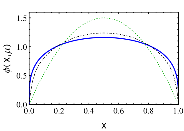
Figure 1: Pion’s PDA: [Solid, blue] $\phi(x,\mu=2\;\mbox{GeV})$. [Dot-dashed, black] ERBL evolution to $\phi(x,\mu=\sqrt{50}\;\mbox{GeV})$. [Green, dotted] Asymptotic PDA, $\phi_{asy}(x)=6x(1-x)$. As we can see, the broad concave PDA, $\phi(x,\mu=2\;\mbox{GeV})$, slowly approaches to its asymptotic form with increasing momentum scale.

From figure 1, we see that pion’s PDA at resolution scale $\mu=2$ GeV, $\phi(x,\mu=2\;\mbox{GeV})$, slowly evolves to its asymptotic form. Evolution enables the dressed-quark and antiquark degrees of freedom, in terms of which the wave function is expressed at a given scale, to split into less well-dressed partons via the addition of gluons and sea quarks in the manner prescribed by QCD dynamics. The connection of $\phi(x,\mu)$ with $G(Q^{2})$ is given by the leading twist expression for the transition form factor:

$$G(Q^{2})=4\pi^{2}f_{\pi}\int_{0}^{1}dxT_{H}(x,Q^{2},\alpha(\mu);\mu)\phi(x,\mu)\;,$$ (11)

where $T_{H}(\mu)$ is the photon-quark-antiquark scattering amplitude at some scale $\mu$. One expects to reach the asymptotic limit from below, otherwise one would have to explain why $G(Q^{2})$ grows bigger and then decreases towards $2f_{\pi}$. QCD is not known to have an additional scale to set in at a higher $Q^{2}$ to make this happen. Only logarithmic corrections have a minor role to play. We shall see that the evolution of $\phi(x,\mu)$ is crucial in understanding the asymptotic behavior of the pion transition form factor. Further details of pion’s PDA can be found in Javier Cobos’ contribution to this proceedings volume and in [7].

4 Results and Conclusions

4.1 Results

Our main result is depicted in figure 2. We obtain an interaction radius of $r_{\pi^{0}}=0.68$ fm, which is practically identical to the one computed in [8] within the same scheme. The Abelian anomaly, namely $2f_{\pi}G(Q^{2}=0)=1$, is satisfied; the asymptotic limit, $2f_{\pi}$, is reached from below except for a logarithmic miss-match. Our result agrees fairly well with all available data below $Q^{2}<10$ GeV², and with Belle data at large $Q^{2}$ scales. However, it fails to reconcile with the data reported by the Babar collaboration.

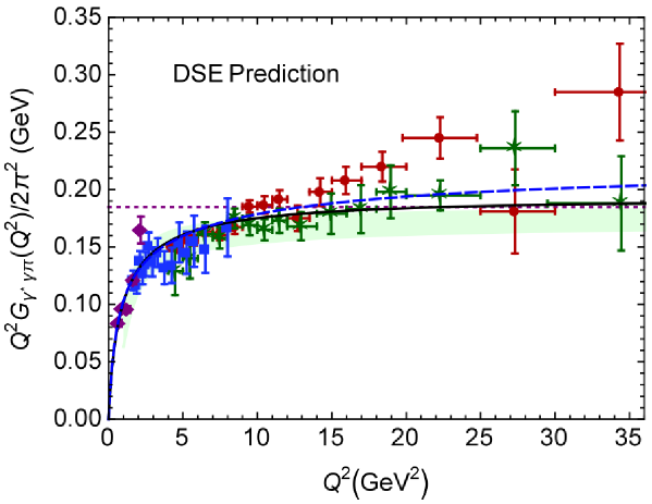
Figure 2: Pion’s transition form factor: [Solid, black] DSE Prediction obtained with the ERBL evolution of pion BSA. [Dashed, blue] DSE Prediction without evolution at frozen scale $\mu=2\;\mbox{GeV}$. Data: [Circles, red] Babar [3], [Diamonds, purple] CELLO [1], [Squares, blue] CLEO [2], [Stars, green] Belle [4]. The (green) shaded band is described in [13].

From figure 2, we see that $G(Q^{2})$ exceeds (logarithmically) the asymptotic limit $2f_{\pi}$, although we expected such limit to be reached from below. However, as mentioned earlier, the growth is only logarithmic, and at some point, it settles onto the value $2f_{\pi}$. This discrepancy originates from the failure of the rainbow-ladder (RL) truncation to reproduce the complete set of gluon and quark splitting effects contained in QCD and hence its inability to fully express interferences between the anomalous dimensions of those $n$-point Schwinger functions which are relevant in the computation of a given scattering amplitude.

4.2 Conclusions

We describe a computation of the pion transition form factor, in which all elements employed are determined by the solutions of the QCD’s DSEs, obtained in the RL truncation.

• The novel analysis techniques made it possible to compute $G(Q^{2})$, on the entire domain of space-like momenta, in a continuum framework directly connected to QCD.

• Our work unifies the description and explanation of this transition with the charged pion electromagnetic form factor and its PDA.

• This enables us to demonstrate that a fully self-contained and consistent treatment can readily connect a pion PDA, that is a broad and concave function at the hadronic scale, with the perturbative QCD prediction for the transition form factor in the hard photon limit.

Full discussion and details are found in our work in [9].

5 Acknowledgements

I want to acknowledge the organizing committee for the financial support and my collaborators in [9] for fruitful discussions.

References

References

- [1] H. J. Behrend et al. [CELLO Collaboration], Z. Phys. C 49, 401 (1991). doi:10.1007/BF01549692
- [2] J. Gronberg et al. [CLEO Collaboration], Phys. Rev. D 57, 33 (1998) doi:10.1103/PhysRevD.57.33 [hep-ex/9707031].
- [3] B. Aubert et al. [BaBar Collaboration], Phys. Rev. D 80, 052002 (2009) doi:10.1103/PhysRevD.80.052002 [arXiv:0905.4778 [hep-ex]].
- [4] S. Uehara et al. [Belle Collaboration], Phys. Rev. D 86, 092007 (2012) doi:10.1103/PhysRevD.86.092007 [arXiv:1205.3249 [hep-ex]].
- [5] G. P. Lepage and S. J. Brodsky, Phys. Rev. D 22, 2157 (1980). doi:10.1103/PhysRevD.22.2157
- [6] P. Maris and P. C. Tandy, Phys. Rev. C 65, 045211 (2002) doi:10.1103/PhysRevC.65.045211 [nucl-th/0201017].
- [7] L. Chang, I. C. Cloet, J. J. Cobos-Martinez, C. D. Roberts, S. M. Schmidt and P. C. Tandy, Phys. Rev. Lett. 110, no. 13, 132001 (2013) doi:10.1103/PhysRevLett.110.132001 [arXiv:1301.0324 [nucl-th]].
- [8] L. Chang, I. C. Cloët, C. D. Roberts, S. M. Schmidt and P. C. Tandy, Phys. Rev. Lett. 111, no. 14, 141802 (2013) doi:10.1103/PhysRevLett.111.141802 [arXiv:1307.0026 [nucl-th]].
- [9] K. Raya, L. Chang, A. Bashir, J. J. Cobos-Martinez, L. X. Gutiérrez-Guerrero, C. D. Roberts and P. C. Tandy, Phys. Rev. D 93, no. 7, 074017 (2016) doi:10.1103/PhysRevD.93.074017 [arXiv:1510.02799 [nucl-th]].
- [10] R. Delbourgo and P. C. West, J. Phys. A 10, 1049 (1977). doi:10.1088/0305-4470/10/6/024
- [11] S. x. Qin, L. Chang, Y. x. Liu, C. D. Roberts and D. J. Wilson, Phys. Rev. C 84, 042202 (2011) doi:10.1103/PhysRevC.84.042202 [arXiv:1108.0603 [nucl-th]].
- [12] A. V. Efremov and A. V. Radyushkin, Phys. Lett. B 94, 245 (1980). doi:10.1016/0370-2693(80)90869-2
- [13] A. P. Bakulev, S. V. Mikhailov, A. V. Pimikov and N. G. Stefanis, Phys. Rev. D 86, 031501 (2012) doi:10.1103/PhysRevD.86.031501 [arXiv:1205.3770 [hep-ph]].