Coherent dynamics of V-type systems driven by time-dependent incoherent radiation

Abstract

Light induced processes in nature occur by irradiation with slowly turned-on incoherent light. The general case of time-dependent incoherent excitation is solved here analytically for V-type systems using a newly developed master equation method. Clear evidence emerges for the disappearance of radiatively induced coherence as turn-on times of the radiation exceed characteristic system times. The latter is the case, in nature, for all relevant dynamical time scales for other than nearly degenerate energy levels. We estimate that, in the absence of non-radiative relaxation and decoherence, turn-on times slower than 1 ms (still short by natural standards) induce Fano coherences between energy eigenstates that are separated by less than 0.9 cm^-1.

I Introduction

A number of femtosecond laser spectroscopy studies Tiwari et al. (2013); Collini et al. (2010); Engel et al. (2007); Hau et al. (1999) on components of light harvesting systems, such as the Fenna-Matthews-Olson (FMO) or PC645 photosynthetic complexes, show that irradiation with fs pulses results in coherent molecular energy transfer dynamics. These observations have been interpreted as demonstrating a role for quantum coherent dynamics in biological systems. However, as has been repeatedly argued Grinev and Brumer (2015); Tscherbul and Brumer (2015); Chenu et al. (2015); Tscherbul and Brumer (2014a); Sadeq and Brumer (2014); Olšina et al. (2014); Tscherbul and Brumer (2014b); Brumer and Shapiro (2012); Pachón and Brumer (2012); Mančal and Valkunas (2010); Ou et al. (2008); Agarwal and Menon (2001); Jiang and Brumer (1991) both formally and computationally, the response of a molecule to coherent laser light is dramatically different from that to natural incoherent radiation, such as sunlight. For example, in the absence of a decohering environment the pulsed laser case shows persistent molecular coherences, whereas the incoherent case yields a complex mixture of molecular energy eigenstates Tscherbul and Brumer (2014a); Dodin et al. (2016). These results cast doubt on the relevance of the experimentally observed molecular coherences to natural light induced and light harvesting processes.

Such studies, barring one Grinev and Brumer (2015) have all relied upon the sudden turn-on of the radiation, which is both unnatural and which generates initial coherence due to the abrupt turn-on of the light. That is, they focused on the fate of coherences after they were generated by sudden turn-on of the radiation. However, natural turn-on of light (e.g. sunrise for photosynthesis, or the blinking of an eye for vision) is very slow by comparison with molecular time scales, motivating further studies of the time evolution of systems subject to time dependent incoherent excitation, and of the associated Fano coherences discussed below. This study is carried out here on the generic V-system, analytically exposing the dependence of the system evolution and the associated coherences on the turn-on time. The results clearly show that the slower the turn-on time, the less the generated molecular coherences. In particular, with natural turn-on times, no molecular coherences will appear between other than near-degenerate levels. For example, with turn-on times on the order of 1 ms, which is still very short compared to natural turn-on times, coherences will be established only between levels spaced by 0.9 cm^-1. A one second turn-on will only induce coherences in levels spaced by $9\times 10^{-4}$ cm^-1.

To consider such coherent effects rigorously, we examine the most general picture of weak-field incoherent light-matter interactions. This is given by the Bloch-Redfield (BR) master equations, in which the populations and coherences of a reduced density matrix are treated on an equal footing Cohen-Tannoudji et al. (1992). The Pauli rate law equations underlying, for example, the Einstein theory for excitation by incoherent light Loudon (2000), can be obtained from the BR theory by neglecting the non-secular terms that couple populations and coherences. However, these non-secular terms are responsible for Fano interference between different incoherent excitation pathways Fleischhauer et al. (1992); Kozlov et al. (2006); Agarwal (1974) The existence of Fano coherences in incoherently driven systems has sparked considerable interest in the context of naturally occurring LHC’s and artificial photovoltaics Fleischhauer et al. (1992); Kozlov et al. (2006); Kiffner et al. (2010) where it has been proposed as a mechanism for enhancing the efficiency of quantum heat engines Dorfman et al. (2013); scu .

The Fano coherences differ significantly in origin from the coherences induced by coherent light. As shown below, they can be understood most easily in terms of a number state picture where absorption of light with frequency $\omega=\omega_{i}$ leads a system in the ground state $|g\rangle$ to make a transition to the excited statesx $|e_{i}\rangle$ and gain phase according to the complex phase of the corresponding transition dipole moment Dodin et al. (2016). For simplicity assume that the transition dipole moments are real and positive. The Fano coherences arise due to simultaneous excitation from the ground state to both excited states, producing a coherent in-phase superposition of the excited states. In contrast, the coherences arising from excitation of the system with coherent sources are a consequence of the phase relations between the transition frequencies. In the number state (photon) picture, coherent light is given by a coherent superposition of number states which contains the phase information as coherences between the number states at the corresponding frequencies. The radiation field coherences can then be “transferred” to the system through the dipole interaction.

Our previous work has explored the role of the Fano coherences in the dynamical evolution of the V-system in the weak pumping limit Tscherbul and Brumer (2014a); Dodin et al. (2016). We have derived the Bloch-Redfield equations for a general class of multilevel systems Tscherbul and Brumer (2015) and identified the parameter dependence of the dynamical evolution of the V-system Dodin et al. (2016). Here, these studies are significantly extended by considering the regime of non-stationary time-dependent incoherent radiation. Section II develops a model for a time-dependent field which is then used to generalize the Bloch-Redfield equations to the case of time-dependent fields in Section III. Section IV uses the BR equations to consider a weakly pumped V-system and presents the general analytical solution, which is examined more closely for the limiting cases of a closely spaced $\Delta\ll\gamma$ system in Section V and a system with wide level spacing $\Delta\gg\gamma$ in Section VI, where $\Delta$ is the excited state splitting and $\gamma$ is the rate of spontaneous emission. Finally, Section VIII summarizes our results.

Note that this paper deals with the molecular coherences generated by the incident light. Those associated with, for example, donor excitation in a donor-acceptor system, briefly discussed in Grinev and Brumer (2015), will be discussed in detail elsewhere Tscherbul and Brumer ; Dodin et al. . Further, these studies do not include, but do motivate including, a second bath that would model, e.g., a bosonic environment. In that case, where the system is coupled to two baths, the long time steady state is a "transport problem", with flow of energy from the radiation field to the second bath. Studies of this kind, which would extend work such as that in Ref. Pachón and Brumer (2013), are in progress.

II Modelling the Time-Dependent Field

II.1 Properties of Field Dynamics

In this section, we first consider a model for a time varying radiation field corresponding to the slow turn on of incoherent light (e.g., a thermal field attenuated by a variable filter), that is an isotropic unpolarized radiation field with constant frequency distribution but time varying intensity. Furthermore, let the radiation field be diagonal in the number state representation at all times.

The isotropy and unpolarized property is straightforward to implement through the following relationship, enforced at all times $t$ and for all non-negative integers $m$:

$${\langle\hat{n}_{\bm{j}\lambda}^{m}\rangle(t)}={\langle\hat{n}_{\bm{k}\mu}^{m}\rangle(t)}\mbox{; if }|\bm{j}|=|\bm{k}|$$ (1)

where $\hat{n}_{\bm{j}\lambda}$ is the number operator for the field mode with wave vector $\bm{j}$ and linear polarization $\lambda=1,2$ and $\langle\hat{A}\rangle(t)$ is the expectation value of the field operator $\hat{A}$. That is, Eq. 1 states that all statistical moments, $m$, of the field mode depend only on the magnitude of the wave vector and not on its direction or polarization. Therefore, the statistical distribution of all field modes with the same wave vector magnitude is identical, realizing an isotropic and unpolarized field.

The requirement for a time-independent frequency distribution is equivalent to assuming that the temperature of a blackbody source does not change. That is,

$$\frac{\langle\hat{n}_{\bm{j}\lambda}\rangle(t)}{\langle\hat{n}_{\bm{k}\mu}\rangle(t)}=Constant\mbox{ for all }t>0$$ (2)

This leads to a source with time-independent bandwidth, $\Delta\omega$, since the bandwidth is a property of the frequency distribution. Consequently, this leads to a time-independent coherence time $\tau_{c}$ for all $t>0$ since $\tau_{c}\Delta\omega\sim 1$ Scully and Zubairy (1997); Mandel and Wolf (1995).

The time-dependence of the field is characterized by the varying intensity of the incident light. Consider the intensity operator of a multimode field:

$$\hat{I}=\bm{\hat{E}}^{(-)}\cdot\bm{\hat{E}}^{(+)}=\left(\sum_{\bm{k}\lambda}\bm{\epsilon}_{\bm{k}\lambda}\xi_{k}\hat{a}_{\bm{k}\lambda}e^{i\nu_{k}t}\right)\cdot\left(\sum_{\bm{j}\mu}\bm{\epsilon}_{\bm{j}\mu}\xi_{j}\hat{a}^{\dagger}_{\bm{j}\mu}e^{-i\nu_{j}t}\right)$$ (3)

For a given field mode with wavevector $\bm{k}$ and linear polarization $\lambda=1,2$, $\hat{a}_{\bm{k}\lambda}$ and $\hat{a}_{\bm{k}\lambda}^{\dagger}$ are the annihilation and creation operators, $\bm{\epsilon}_{\bm{k},\lambda}$ is the corresponding polarization vector, $\nu_{k}$ is the frequency of the field mode and $\xi_{k}=(\hbar\nu_{k}/2\epsilon_{0}V_{ph})^{1/2}$ is the electric field per photon, where $V_{ph}$ is the photon volume. Here, $\bm{\hat{E}}^{(\pm)}$ are the positive and negative frequency components of the electric field. For an unpolarized isotropic field, Eq. 3 reduces to

$$\hat{I}=\sum_{k}2|\xi_{k}|^{2}\left(\hat{n}_{k}+\frac{1}{2}\right)$$ (4)

where $\hat{n}_{k}=\sum_{\lambda}\sum_{\bm{j}:|j|=|k|}\hat{n}_{\bm{j}\lambda}$ is the total occupation number of field modes with wave vector magnitude $k$. The only part of Eq. 4 that depends on the field properties is the total occupation number operator. Therefore, to obtain a time-dependent intensity expectation value, the radiation field density matrix must change over time such that

$$n_{\bm{k}\lambda}(t)=\langle\hat{n}_{\bm{k}\lambda}\rangle(t)=\operatorname{Tr_{R}}\left\{\hat{n}_{\bm{k}\lambda}\hat{\rho}_{R}(t)\right\}=n_{\bm{k}\lambda}f(t)$$ (5)

where $\operatorname{Tr_{R}}$ is the trace over the radiation field. The turn on function must be identical for all modes due to the restrictions from Eqs. 1 and 2. For computational simplicity we consider a slow turn on envelope of the form

$$f(t)=1-e^{-\alpha t}$$ (6)

where $\alpha$ is a constant characterizing the turn on rate, with a corresponding turn on time scale $\tau_{r}=1/\alpha$. Appendix A outlines the generalization of the results for arbitrary turn on functions through their expansion in a Laplace-like basis.

Finally, Eq. (5) gives a source that is quasi-canonical in that no coherences exist between number states of the bath. Intuitively, this corresponds to a bath that is similar to the incoherent fields studied previously Dodin et al. (2016) (e.g. Blackbody radiation field) at each instant in time.

II.2 Realizing the Time-Dependent Field

Since our interest is in the system that is irradiated by the incoherent light, the latter acts as an time-dependent external bath that is coupled to the system. Treating a time-dependent bath within the standard framework of open quantum systems poses challenges that are not present in the stationary field case. That is, in standard density matrix theory the System-Bath composite is assumed to be closed, allowing for the development of the density matrix theory in terms of the Unitary Hamiltonian evolution of the total state vector in the joint Hilbert Space of the system and bath Breuer and Petruccione (2007). However, the time evolution of the radiation field described in Sec. IIA does not arise through the typical Hamiltonian evolution of a system $+$ bath.

Instead, we need to consider an additional environment $E$ coupled to the radiation bath, but not to the system, in the Born-Markov approximation, and let the radiative bath be coupled to the system in the Born-Markov regime. This set up is sketched in Fig. 1. Intuitively, the environment corresponds to the physical system that produces the dynamics of the field on the system. This hierarchical approach has the benefit of allowing the use of the standard approach to open quantum systems Breuer and Petruccione (2007); Blum (2012), since the system-bath-environment composite is closed and hence evolves according to unitary Hamiltonian dynamics. To obtain well posed problems for the dynamics of the bath and the system, the system-bath-environment is assumed to be initially in a separable state $\hat{\rho}_{0}=\hat{\rho}_{S}\otimes\hat{\rho}_{R}\otimes\hat{\rho}_{E}$.

Fig. 1: A schematic representation of the coupling between the molecular system, S, radiation bath, R, and environment, E. The system and environment are not directly coupled. The system-bath interaction, $V_{SR}$, and bath-environment interaction, $V_{RE}$ satisfy the Born-Markov approximation.

The Born approximation to the system-bath coupling implies that the influence of the system on the bath dynamics is negligible. Therefore, we can treat the environment-bath composite using the standard approach to computing the reduced dynamics of the bath. We can select the environment and interaction potential such that the dynamics of the bath correspond to that discussed in Sec. IIA. In the resultant picture, the properties of the bath operators can be treated by exact analogy to the system operators in a typical system-bath case. For example, the two time correlation function for two Schrödinger Operators, $\hat{A}$ and $\hat{B}$, on the bath Hilbert Space, $\mathcal{H}_{R}$ is given by:

$$\langle\hat{A}(s)\hat{B}(t)\rangle=\operatorname{Tr_{R}}\left\{\hat{A}\hat{U}(s,t)\hat{B}\hat{U}(t,0)\hat{\rho}_{R}(0)\right\}$$ (7)

where $\hat{\rho}_{R}(0)$ is the initial state of the bath, assumed to be the vacuum state in our case, and $\hat{U}(s,t)$ is the bath propagation operator from time $s$ to time $t$. After obtaining the bath dynamics, the resulting time-varying density matrix can be used to determine the dynamics of the system while neglecting any further role of the environment, E.

III Derivation of the Bloch-Redfield Equations for Time-Dependent Baths

Traditional master equations assume a time independent bath. Therefore, to treat turn-on effects, we derive a generalization to the time dependent bath. Consider a multilevel system interacting with a quantized incoherent radiation field, as described in Sec. II, under the dipole and rotating wave approximations. Such a system is characterized by the total Hamiltonian

$$\hat{H}_{T}=\hat{H}_{S}+\hat{H}_{R}+\hat{H}_{E}+\hat{V}_{SR}+\hat{V}_{RE}$$ (8)

where $\hat{H}_{S}=\sum_{i}E_{i}|i\rangle\langle i|$ is the system Hamiltonian, $\hat{H}_{R}=\sum_{\bm{k}\lambda}\hbar\nu_{k}\hat{a}_{\bm{k}\lambda}\hat{a}_{\bm{k}\lambda}^{\dagger}$ is the radiation bath Hamiltonian and $\hat{H}_{E}$ is the environment Hamiltonian. The operator $\hat{V}_{RE}$ is the bath-environment interaction potential. The bosonic creation and annihilation operators of the field mode with wavevector $\bm{k}$, frequency $\nu_{k}$ and polarization $\lambda=1,2$ are given by $\hat{a}_{\bm{k}\lambda}^{\dagger}$ and $\hat{a}_{\bm{k}\lambda}$ respectively. $\hat{V}_{SR}$ is the system-bath interaction potential given by Scully and Zubairy (1997)

$$\hat{V}_{SR}=-\bm{\hat{\mu}}\cdot\sum_{\bm{k},\lambda}\left(\frac{\hbar\nu_{k}}{2\epsilon_{0}V}\right)^{1/2}\bm{\epsilon}_{\bm{k}\lambda}(\hat{a}_{\bm{k}\lambda}-\hat{a}^{\dagger}_{\bm{k}\lambda})$$ (9)

where $V$ is the quantization volume, $\bm{\hat{\mu}}$ is the dipole moment operator of the system and $\bm{\epsilon}_{\bm{k}\lambda}$ is the polarization vector of the field mode with wavevector $\bm{k}$ and polarization $\lambda$.

The bath-environment interaction potential and environment Hamiltonian are not specified, but are chosen to produce the bath dynamics discussed in Sec. II. Under the Born-Markov approximation, the system does not contribute to the bath evolution, induced by its interaction with the environment. In other words, the effects of $\hat{V}_{SR}^{I}$ and $\hat{H}_{S}$ on the dynamics of the radiation field + environment can be neglected. This produces a density operator, $\hat{\rho}_{RE}$, on the radiation field + environment Hilbert space such that the radiation field density matrix $\hat{\rho}_{R}(t)=\operatorname{Tr_{E}}\hat{\rho}_{RE}$ follows the conditions described in Sec. II, where $\operatorname{Tr_{E}}$ is the trace over the environment $E$.

Transforming Eq. 9 into the interaction picture gives

$$\hat{V}_{SR}^{I}(t)=\hbar\sum_{i\leq j}\sum_{\bm{k}\lambda}g_{\bm{k}\lambda}^{(i,j)}(\hat{a}_{\bm{k}\lambda}|j\rangle\langle i|e^{i(\omega_{ij}-\nu_{k})t}+\mbox{H.c.})$$ (10)

where $g_{\bm{k}\lambda}^{(i,j)}=\left(\frac{\hbar\nu_{k}}{2\epsilon_{0}V}\right)^{\frac{1}{2}}\frac{\bm{\mu}_{ij}\cdot\bm{\epsilon}_{\bm{k}\lambda}}{\hbar}$ are the light-matter coupling constants and $\bm{\mu}_{ij}=\langle i|\bm{\hat{\mu}}|j\rangle$ are the transition dipole matrix elements, assumed real.

The equations of motion of the system-bath composite $\hat{\rho}=\hat{\rho}_{S}\otimes\hat{\rho}_{R}$ in the interaction picture are given by the Liouville Von-Neuman equation Breuer and Petruccione (2007); Blum (2012)

$$\dot{\hat{\rho}}(t)=-i[\hat{V}_{SR}^{I}(t),\hat{\rho}(0)]-\int^{t}_{0}dt^{\prime}[\hat{V}_{SR}^{I}(t),[\hat{V}_{SR}^{I}(t^{\prime}),\hat{\rho}(t^{\prime})]]$$ (11)

If the system and bath are initially in a separable state $\hat{\rho}(0)=\hat{\rho}_{S}(0)\otimes\hat{\rho}_{R}(0)$, the Born approximation states that, for weak system-bath coupling (which is valid for the natural light excitation of LHC’s) they remain in a separable state at all times. Furthermore, the small system produces no back reaction on the large bath.

Applying the Born approximation to Eq. 11 and tracing over the bath coordinates gives the equations of motion for the reduced system density matrix $\hat{\rho}_{S}$:

$$\dot{\hat{\rho}}_{S}(t)=-i\textrm{Tr}_{R}[\hat{V}_{SR}^{I}(t),\hat{\rho}_{S}(0)\otimes\hat{\rho}_{R}(0)]-\int^{t}_{0}dt^{\prime}\textrm{Tr}_{R}[\hat{V}_{SR}^{I}(t),[\hat{V}_{SR}^{I}(t^{\prime}),\hat{\rho}_{S}(t^{\prime})\otimes\hat{\rho}_{R}(t^{\prime})]]$$ (12)

where $\text{Tr}_{R}$ denotes a trace over the radiation field. While this equation is similar to the standard master equation for stationary baths Breuer and Petruccione (2007); Blum (2012), the radiation field density matrix now carries an explicit time-dependence due to the interaction with the environment.

Given Eq. (10), the double commutator in Eq. 12 gives products of $\hat{V}_{SR}^{I}$ at two different times, with a typical term of the form:

$$\int^{t}_{0}dt^{\prime}\sum_{i\leq j}\sum_{l\leq m}\sum_{\bm{k}\lambda}\sum_{\bm{k^{\prime}}\lambda^{\prime}}g_{\bm{k}\lambda}^{(i,j)}g_{\bm{k^{\prime}}\lambda^{\prime}}^{(l,m)}\langle\hat{a}_{\bm{k}\lambda}\hat{a}^{\dagger}_{\bm{k^{\prime}}\lambda^{\prime}}\rangle(t^{\prime})\hat{\sigma}_{i,j}\hat{\sigma}_{m,l}\hat{\rho}_{S}(t^{\prime})e^{-i(\omega_{ij}-\nu_{k})t^{\prime}+i(\omega_{lm}-\nu_{k^{\prime}})t}~{}.$$ (13)

Here $\hat{\sigma}_{i,j}=|i\rangle\langle j|$ is the “quantum jump operator” from state $|j\rangle$ to state $|i\rangle$.

Using the commutator algebra of bosonic creation and annihilation operators, and the identity $\hat{a}_{\bm{k}\lambda}\hat{a}^{\dagger}_{\bm{k^{\prime}}\lambda^{\prime}}=(1+\hat{n}_{\bm{k}\lambda})\delta_{\bm{k},\bm{k^{\prime}}}\delta_{\lambda,\lambda^{\prime}}$, the trace over the bath in Eq. 13 is obtained as:

$$\langle\hat{a}_{\bm{k}\lambda}\hat{a}^{\dagger}_{\bm{k^{\prime}}\lambda^{\prime}}\rangle(t)=Tr_{R}\left\{\hat{a}_{\bm{k}\lambda}\hat{a}^{\dagger}_{\bm{k^{\prime}}\lambda^{\prime}}\hat{\rho}_{R}(t)\right\}=\delta_{\bm{k},\bm{k^{\prime}}}\delta_{\lambda,\lambda^{\prime}}\left(1+n_{\bm{k}\lambda}(t)\right)$$ (14)

Here we have used the normalization of the bath density matrix $\textrm{Tr}_{R}\{\hat{\rho}_{R}(t)\}=1$, Eq. 5, and the linearity of the trace. Substituting Eq. 14 into Eq. 13 gives

$$\int^{t}_{0}dt^{\prime}\sum_{i\leq j}\sum_{l\leq m}\sum_{\bm{k}\lambda}g_{\bm{k}\lambda}^{(i,j)}g_{\bm{k}\lambda}^{(l,m)}(1+n_{\bm{k}\lambda}(t^{\prime}))\hat{\sigma}_{i,j}\hat{\sigma}_{m,l}\hat{\rho}_{S}(t^{\prime})e^{-i(\omega_{ij}-\nu_{k})t^{\prime}+i(\omega_{lm}-\nu_{k})t}$$ (15)

Taking the continuum limit of the $\bm{k}$ summation

$$\sum_{\bm{k}}\to\frac{2V}{(2\pi)^{3}}\int^{2\pi}_{0}d\phi\int^{\pi}_{0}d\theta\sin(\theta)\int^{\infty}_{0}dk\,k^{2}$$ (16)

and noting that for an isotropic and unpolarized field $n_{\bm{k}\lambda}$ depends only on $k$ and not on the angular or polarization coordinates, Eq. 15 can be rearranged to yield

$$\frac{1}{8\pi^{3}\epsilon_{0}}\int^{t}_{0}dt^{\prime}\sum_{i\leq j}\sum_{l\leq m}\hat{\sigma}_{i,j}\hat{\sigma}_{m,l}\hat{\rho}_{S}(t^{\prime})e^{-i(\omega_{ij}t^{\prime}-\omega_{lm}t)}\\ \times\left[\sum_{\lambda}\int^{2\pi}_{0}d\phi\int^{\pi}_{0}d\theta\sin(\theta)(\bm{\mu}_{ij}\cdot\bm{\epsilon}_{\bm{k}\lambda})(\bm{\mu}_{lm}\cdot\bm{\epsilon}_{\bm{k}\lambda})\right]\left[\int^{\infty}_{0}dkk^{2}\nu_{k}(1+n_{\bm{k}\lambda}(t^{\prime}))e^{i\nu_{k}(t-t^{\prime})}\right]$$ (17)

The summation over the angular and polarization coordinates in Eq. 17 can be evaluated to give $\bm{\mu}_{ij}\cdot\bm{\mu}_{lm}$. Changing variables from $k$ to $\nu_{k}=ck$, Eq. 17 can be written in the following form:

$$\sum_{i\leq j}\sum_{l\leq m}\frac{\bm{\mu}_{ij}\cdot\bm{\mu}_{lm}}{8\pi^{3}\epsilon_{0}c^{3}}e^{i(\omega_{ij}-\omega_{lm})t}\int^{\infty}_{0}d\nu_{k}\nu_{k}^{3}\int^{t}_{0}dt^{\prime}e^{i(\omega_{ij}-\nu_{k})(t-t^{\prime})}(1+n_{\bm{k}\lambda}(t^{\prime}))\hat{\sigma}_{i,j}\hat{\sigma}_{l,m}\hat{\rho}_{S}(t^{\prime})$$ (18)

The exponential factor in the integrand oscillates rapidly at $\nu_{k}\neq\omega_{ij}$, so provided that $n_{\bm{k}\lambda}$ varies slowly near $\omega_{ik}$ at all times, we can make the Wigner-Weisskopff approximation by setting Scully and Zubairy (1997)

$$\int^{\infty}_{0}d\nu_{k}\nu_{k}^{3}e^{-i\nu_{k}(t-t^{\prime})}\rightarrow\omega_{ij}^{3}\int_{0}^{\infty}d\nu_{k}e^{-i\nu_{k}(t-t^{\prime})}$$ (19)

giving

$$\sum_{i\leq j}\sum_{l\leq m}\frac{\bm{\mu}_{ij}\cdot\bm{\mu}_{lm}\omega_{ij}^{3}}{8\pi^{3}\epsilon_{0}c^{3}}e^{i(\omega_{ij}-\omega_{lm})t}\int^{t}_{0}dt^{\prime}(1+n_{\bm{k}\lambda}(t^{\prime}))\hat{\sigma}_{i,j}\hat{\sigma}_{m,l}\hat{\rho}_{S}(t^{\prime})e^{i\omega_{ij}t^{\prime}}\int^{\infty}_{0}d\nu_{k}e^{-i\nu_{k}(t-t^{\prime})}$$ (20)

The $\nu_{k}$ integral in Eq. 20 can now be evaluated as $\pi\delta(t-t^{\prime})+iP(1/(t-t^{\prime}))$ where $P$ denotes the Cauchy Principal Part. Neglecting the small Lamb shift due to the imaginary part of Eq. (19), and doing the time integral gives

$$\sum_{i\leq j}\sum_{l\leq m}\frac{\mu_{ij}\mu_{lm}p_{ij,lm}\omega_{ij}^{3}}{8\pi^{2}\epsilon_{0}c^{3}}(1+n_{k_{ij}\lambda}(t))\hat{\sigma}_{ij}\hat{\sigma}_{m,l}\hat{\rho}_{S}(t)e^{i(\omega_{lm}-\omega_{ij})t}$$ (21)

where alignment parameters, $p_{ij,lm}$, for the transition dipole moments have been defined:

$$p_{ij,lm}=\frac{\bm{\mu}_{ij}\cdot\bm{\mu}_{lm}}{\mu_{ij}\mu_{lm}}$$ (22)

Transforming Eq. 21 back into the Schrödinger picture eliminates the oscillating phase factor and yields the same master equations as previously reported for stationary fields Tscherbul and Brumer (2015), but with time dependent occupation numbers. That is, following the same approach as in Ref. Tscherbul and Brumer (2015) we arrive at the same master equations [Eq. (17) in Ref. Tscherbul and Brumer (2015)] with the following substitution.

$$r_{ij}=\gamma_{ij}\overline{n}_{\omega_{ij}}\to r_{ij}(t)=\gamma_{ij}\overline{n}_{\omega_{ij}}(t)$$ (23)

where $r_{ij}(t)$ is the pumping rate from level $g_{i}$ in the ground state manifold to state $e_{j}$ in the excited state manifold.

IV V-System Master Equations

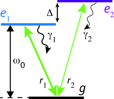
Fig. 2: Schematic representation of a V-type System. $\Delta$ is the excited state splitting, $\gamma_{i}$ is the radiative line-width, and $r_{i}$ is the incoherent pumping rate of excited state $|e_{i}\rangle$.

Consider now a V-system with one ground state and two excited states (as shown in Fig. 2) coupled to a time dependent incoherent radiation field. Since there is only one ground state in the V-system, we suppress the first index ($i$) which specifies the ground state in the pumping rate $r_{ij}(t)$ and spontaneous emission rate $\gamma_{ij}$. That is $r_{ij}(t)\to r_{j}(t)$ gives the pumping rate from the ground state $g$ to the excited state $e_{j}$ and $\gamma_{ij}\to\gamma_{j}$ gives the spontaneous decay rate from excited state $e_{j}$ to the ground state $g$. The master equation for such a system is given by

$$\dot{\rho}_{e_{j}e_{j}}=-(r_{j}(t)+\gamma_{j})\rho_{e_{j}e_{j}}+r_{j}(t)\rho_{gg}-p(\sqrt{r_{1}(t)r_{2}(t)}+\sqrt{\gamma_{1}\gamma_{2}})\rho_{e_{1}e_{2}}^{R}$$ (24a)

$$\begin{split}\dot{\rho}_{e_{1}e_{2}}=&-\frac{1}{2}(r_{1}(t)+r_{2}(t)+\gamma_{1}+\gamma_{2})\rho_{e_{1}e_{2}}-i\rho_{e_{1}e_{2}}\Delta\\ &+\frac{p}{2}\sqrt{r_{1}(t)r_{2}(t)}(2\rho_{gg}-\rho_{e_{1}e_{1}}-\rho_{e_{2}e_{2}})-\frac{p}{2}\sqrt{\gamma_{1}\gamma_{2}}(\rho_{e_{1}e_{1}}+\rho_{e_{2}e_{2}})\end{split}$$ (24b)

where $\rho_{e_{1}e_{2}}^{R}$ is the real part of the off-diagonal (coherence) density matrix element between levels $e_{1}$ and $e_{2}$. In Eq. 24b, spontaneous emission processes are governed by the radiative decay widths of the excited states, $\gamma_{i}=\omega_{ge_{i}}^{3}|\mu_{ge_{i}}|^{2}/(3\pi\epsilon_{0}c^{3})$, $\Delta=\omega_{e_{1}e_{2}}$ gives the excited state splitting and $p=\bm{\mu}_{ge_{1}}\cdot\bm{\mu}_{ge_{2}}/(|\mu_{ge_{1}}||\mu_{ge_{2}}|)$ measures the alignment of the $|g\rangle\leftrightarrow|e_{i}\rangle$ transition dipole moments, $\bm{\mu}_{ge_{i}}$. Absorption and stimulated emission processes are parametrized by time-dependent incoherent pumping rates of the $|g\rangle\leftrightarrow|e_{i}\rangle$ transitions, $r_{i}(t)=\gamma_{i}\bar{n}(t)$. Here we neglect environment-induced dephasing and relaxation processes, assuming that the rates of excited state relaxation and dephasing are small compared to those of the radiative processes (absorption, decay and stimulated emission) Dodin et al. (2016). These effects can, however be included by generalizing this approach Tscherbul and Brumer (2014a).

As in the case of stationary pumping rates Dodin et al. (2016), applying the conservation of population constraint, $\rho_{gg}=1-\rho_{e_{1}e_{1}}-\rho_{e_{2}e_{2}}$, and transforming into the Liouville space representation with state vector $\bm{x}=[\rho_{e_{1}e_{1}},\rho_{e_{2}e_{2}},\rho_{e_{1}e_{2}}^{R},\rho_{e_{1}e_{2}}^{I}]^{T}$ yields Eq. 24b in a vector form:

$$\frac{d}{dt}\bm{x}=A(t)\bm{x}+\bm{d}(t)$$ (25a)

$$A(t)=\left(\begin{array}[]{cccc}-(2r_{1}(t)+\gamma_{1})&-r_{1}(t)&-p\sqrt{\gamma_{1}\gamma_{2}}\left(1+\bar{n}(t)\right)&0\\ -r_{2}(t)&-(2r_{2}(t)+\gamma_{2})&-p\sqrt{\gamma_{1}\gamma_{2}}\left(1+\bar{n}(t)\right)&0\\ -\frac{p\sqrt{\gamma_{1}\gamma_{2}}}{2}\left(1+3\bar{n}(t)\right)&-\frac{p\sqrt{\gamma_{1}\gamma_{2}}}{2}\left(1+3\bar{n}(t)\right)&-\bar{\gamma}(1+\bar{n}(t))&\Delta\\ 0&0&-\Delta&-\bar{\gamma}(1+\bar{n}(t))\end{array}\right)$$ (25b)

$$\mathbf{d}(t)=\left(\begin{array}[]{c}r_{1}(t)\\ r_{2}(t)\\ p\sqrt{r_{1}(t)r_{2}(t)}\\ 0\end{array}\right)$$ (25c)

where $\bar{\gamma}=\frac{1}{2}(\gamma_{1}+\gamma_{2})$ is the arithmetic mean of the spontaneous decay rates of the excited state manifold, and we have used the fact that $r_{i}(t)/\gamma_{i}=\bar{n}(t)$.

Rewriting Eq. 25c in the form $\mathbf{d}(t)=[\gamma_{1},\gamma_{2},p\sqrt{\gamma_{1}\gamma_{2}},0]^{T}\bar{n}(t)$ shows that the time-varying field pumps the system to the same statistical mixture, $\rho_{d}$, in the excited manifold as does the stationary field Dodin et al. (2016), where

$$\rho_{d}\propto(1-p)(\gamma_{1}|e_{1}\rangle\langle e_{1}|+\gamma_{2}|e_{2}\rangle\langle e_{2}|)+p|\phi_{+}\rangle\langle\phi_{+}|.$$ (26)

Here $|\phi_{+}\rangle=(1/\sqrt{2\bar{\gamma}})(\sqrt{\gamma_{1}}|e_{1}\rangle+\sqrt{\gamma_{2}}|e_{2}\rangle)$ is an in-phase coherent superposition of excited energy eigenstates. However, in contrast to the stationary field case, the rate of excitation into this statistical mixture varies with time. Hence, although these equations look similar to the stationary case, the time-varying excitation rate in this case produces very different dynamics than one sees in the stationary rate case.

Provided the weak-pumping limit ($\bar{n}(t)\ll 1$) is satisfied at all times, the coefficient matrix $A(t)$ Eq. 25b can be perturbatively expanded in $\bar{n}(t)$. This yields a time-independent coefficient matrix $A^{(0)}$ to zeroth order in $\bar{n}(t)$, allowing the time-dependent contributions to $A(t)$ to be treated through a perturbative expansion:

$$A(t)=A^{(0)}+\bar{n}(t)A^{(1)}$$ (27a)

$$A^{(0)}=\left(\begin{array}[]{cccc}-\gamma_{1}&0&-p\sqrt{\gamma_{1}\gamma_{2}}&0\\ 0&-\gamma_{2}&-p\sqrt{\gamma_{1}\gamma_{2}}&0\\ -\frac{p\sqrt{\gamma_{1}\gamma_{2}}}{2}&-\frac{p\sqrt{\gamma_{1}\gamma_{2}}}{2}&-\bar{\gamma}&\Delta\\ 0&0&-\Delta&-\bar{\gamma}\end{array}\right)$$ (27b)

As a result, this yields a linear system of constant coefficient ordinary differential equations with a time dependent driving term. Applying the initial conditions appropriate to excitation from a molecule in the ground state, $\rho_{gg}(0)=1$ or $\bm{x_{0}}=\bm{0}$, the dynamics of the V-system is given by the variation of parameters solution Boyce and DiPrima (2009)

$$\mathbf{x}=\int^{t}_{0}dse^{A^{(0)}(t-s)}\mathbf{d}(s)\to\sum_{i=1}^{4}\int^{t}_{0}ds(\mathbf{v}_{i}\cdot\mathbf{d}(s))e^{\lambda_{i}(t-s)}\mathbf{v}_{i}$$ (28)

where $\lambda_{i}$ is the $i^{th}$ eigenvalue of $A^{(0)}$ with corresponding eigenvector $\mathbf{v_{i}}$. Eq. 28 relates the eigenvalues, $\{\lambda_{i}\}$, of $A^{(0)}$ to the timescales of the system’s evolution $\tau_{i}=\operatorname{Re}(\lambda_{i})^{-1}$ and to the frequencies of its oscillations $\omega_{i}=\operatorname{Im}(\lambda_{i})$. This solution is similar to that obtained in Dodin et al. (2016) with the crucial modification that $\mathbf{d}(s)$ is explicitly time dependent.

Since $A^{(0)}$ is time independent, its eigenvalues, eigenvectors and normal modes are identical to those calculated in the stationary field case Dodin et al. (2016), with

$$\lambda_{i}=-\bar{\gamma}\pm\Delta_{p}\sqrt{\zeta^{2}-1}\sqrt{\frac{1\pm\sqrt{1+\eta^{2}}}{2}}$$ (29a)

$$\zeta=\frac{\bar{\gamma}}{\Delta_{p}}$$ (29b)

$$\eta=\frac{\Delta|\gamma_{1}-\gamma_{2}|}{|\bar{\gamma}^{2}-\Delta_{p}^{2}|}$$ (29c)

where $\Delta_{p}=\sqrt{\Delta^{2}+(1-p^{2})\gamma_{1}\gamma_{2}}$.

The overdamped ($\Delta_{p}/\bar{\gamma}\ll 1$) and underdamped ($\Delta_{p}/\bar{\gamma}\gg 1$) regimes of a V-system excited by a field with a finite turn on time $\tau_{r}$ of the form Eq. 5 are discussed below. Since $\Delta_{p}\geq\Delta$ where the latter is the excited state level splitting, the overdamped region would be relevant to, e.g., large molecules whereas the underdamped region would correspond, e.g., to small molecules.

V Overdamped Regime $\frac{\Delta_{p}}{\bar{\gamma}}\ll 1$

In the overdamped regime, where $\zeta=\frac{\bar{\gamma}}{\Delta_{p}}\gg 1$ of Eq. 29a, the eigenvalues take the simplified form Dodin et al. (2016)

$$\lambda_{1}=-2\bar{\gamma}$$ (30a)

$$\lambda_{2}=-\frac{\Delta_{p}^{2}}{2\bar{\gamma}}$$ (30b)

$$\lambda_{3,4}=-\bar{\gamma}~{},$$ (30c)

while the normal modes are given by Dodin et al. (2016)

$$\mathbf{v}_{1}\propto[r_{1},r_{2},p\sqrt{r_{1}r_{2}},0]$$ (31a)

$$\mathbf{v}_{2}\propto[r_{2},r_{1},-p\sqrt{r_{1}r_{2}},0]$$ (31b)

$$\mathbf{v}_{3}\propto[0,0,0,1]$$ (31c)

$$\mathbf{v}_{4}\propto[1,-1,-\frac{\gamma_{1}-\gamma_{2}}{p\sqrt{\gamma_{1}\gamma_{2}}},0]~{}.$$ (31d)

Substituting Eqs. 31d and 30c for the eigenvalues and normal modes, and Eq. 5 for the occupation number, into the variation of parameters solution Eq. 28 and doing the exponential integrals yields the V-system dynamics

$$\begin{split}\rho_{e_{i}e_{i}}(t)=\frac{1}{2\bar{\gamma}}&\bigg{\{}\frac{r_{j}}{\frac{\Delta_{p}^{2}}{2\bar{\gamma}}-\alpha}\left[\frac{\Delta_{p}^{2}}{2\bar{\gamma}}\left(1-e^{-\alpha t}\right)-\alpha\left(1-e^{-\frac{\Delta_{p}^{2}}{2\bar{\gamma}}t}\right)\right]\\ &+\frac{r_{i}}{2\bar{\gamma}-\alpha}\left[2\bar{\gamma}\left(1-e^{-\alpha t}\right)-\alpha\left(1-e^{-2\bar{\gamma}t}\right)\right]\bigg{\}}\end{split}$$ (32a)

$$\begin{split}\rho_{e_{1}e_{2}}(t)=\frac{p\sqrt{r_{1}r_{2}}}{2\bar{\gamma}}&\bigg{\{}\frac{1}{\frac{\Delta_{p}^{2}}{2\bar{\gamma}}-\alpha}\left[\frac{\Delta_{p}^{2}}{2\bar{\gamma}}\left(1-e^{-\alpha t}\right)-\alpha\left(1-e^{-\frac{\Delta_{p}^{2}}{2\bar{\gamma}}t}\right)\right]\\ &-\frac{1}{2\bar{\gamma}-\alpha}\left[2\bar{\gamma}\left(1-e^{-\alpha t}\right)-\alpha\left(1-e^{-2\bar{\gamma}t}\right)\right]\bigg{\}}\end{split}$$ (32b)

where $i,j=1,2$ and $i\neq j$ and $r_{i}=\lim_{t\to\infty}r_{i}(t)=\gamma_{i}\bar{n}$ is the steady state incoherent pumping rate. Here $\alpha$, we recall from Eq. 6, defines the turn on time $\tau_{r}=1/\alpha$.

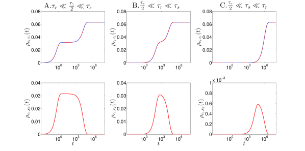
Fig. 3: Evolution of populations and coherences of an overdamped V-system ($\frac{\Delta_{p}}{\bar{\gamma}}\ll 1$) evaluated with aligned transition dipole moments ($p=1$). Here $\gamma_{1}=1.0=\gamma_{2}$ and $\Delta=0.001$. Three different turn on regimes are shown. Panels A show the ultrafast turn on of the field with $\tau_{r}=\times 10^{-3}\tau_{\gamma}$ while Panels B and C show the intermediate ($\tau_{r}=100\tau_{\gamma}=5\times 10^{-5}\tau_{s}$) and slow ($\tau_{r}=20\tau_{s}$) turn on regimes, respectively. Note the difference in y-axis scales for the different coherence plots.

Equations 32a and 32b show that the steady state behavior is given by $\lim_{t\to\infty}\bm{x}(t)=[\bar{n},\bar{n},0,0]$, is independent of $\alpha\neq 0$, and is identical to the steady state obtained for stationary fields Dodin et al. (2016). However, the non-equilibrium behavior of the system and the maximal coherence can be markedly different for time-varying fields, as shown in Fig. 3.

To illustrate this consider a system where the radiation field turn on time $\tau_{r}=1/\alpha$ differs significantly from $\tau_{\gamma}/2=1/2\bar{\gamma}$ and $\tau_{s}=2\bar{\gamma}/\Delta_{p}^{2}$. Since the overdamped regime imposes the inequality $\tau_{s}\gg\tau_{\gamma}/2$, this corresponds to a separation of timescales $\{\tau_{\gamma}/2,\tau_{s},\tau_{r}\}$. There are three possible time-orderings: the sudden turn on ($\tau_{r}\ll\tau_{\gamma}/2\ll\tau_{s}$), the slow turn on ($\tau_{\gamma}/2\ll\tau_{s}\ll\tau_{r}$) and the intermediate ($\tau_{\gamma}/2\ll\tau_{r}\ll\tau_{s}$) regimes.

For the sudden turn on of the field, Eq. 32b simplifies to

$$\rho_{e_{i}e_{i}}(t)=\frac{1}{2\bar{\gamma}}\left[r_{i}\left(1-e^{-2\bar{\gamma}t}\right)+r_{j}\left(1-e^{-\frac{\Delta_{p}^{2}}{2\bar{\gamma}}t}\right)\right]$$ (33a)

$$\rho_{e_{1}e_{2}}(t)=\frac{p\sqrt{r_{1}r_{2}}}{2\bar{\gamma}}\left(e^{-\frac{\Delta_{p}^{2}}{2\bar{\gamma}}t}-e^{-2\bar{\gamma}t}\right)$$ (33b)

under a binomial expansion to lowest contributing order in ${\tau_{r}}/{\tau_{s}}\ll 1$. Equation 33b is independent of $\alpha$ (and hence $\tau_{r}$) and is identical to the expression derived for stationary fields, the $\tau_{r}\to 0$ limit Dodin et al. (2016). The large quasistationary coherences characteristic of this regime can clearly be seen in subplot A of Fig. 3. That is, if the field is turned on faster than the fastest characteristic time scale of the system $\tau_{\gamma}/2=1/2\bar{\gamma}$ then the dynamics of the system are well approximated by the stationary field solution, Eq. 33b. In particular, the coherences approach the same maximal value of $\frac{p\sqrt{r_{1}r_{2}}}{2\bar{\gamma}}$ in the interval $\tau_{\gamma}/2<t<\tau_{s}=\frac{2\bar{\gamma}}{\Delta_{p}^{2}}$ as in the stationary field approximation. In this limit, the field reaches its steady state much faster than the system evolves, and so the very short-lived transient behavior of the field is not reflected in the evolution of the system. Intuitively, in this regime the V-system does not evolve under the transient field. Instead, it evolves only under the steady state field.

By contrast, if the field is turned on very slowly, $\tau_{\gamma}/2\ll\tau_{s}\ll\tau_{r}$, the stationary field solution is a very poor approximation for the system dynamics. Taking a binomial expansion to lowest contributing order in ${\tau_{s}}/\tau_{r}\ll 1$, Eq. 32b can be rewritten as

$$\rho_{e_{i}e_{i}}(t)=\bar{n}\left(1-e^{-\alpha t}\right)$$ (34a)

$$\rho_{e_{1}e_{2}}(t)=\frac{p\alpha\sqrt{r_{1}r_{2}}}{\Delta_{p}^{2}}\left(e^{-\frac{\Delta_{p}^{2}}{2\bar{\gamma}}t}-e^{-\alpha t}\right)$$ (34b)

The dependence on the incoherent pumping rates, $r_{i}$, in Eq. 34b is contained in the mean thermal occupation of the field $\bar{n}=r_{i}/\gamma_{i}$. To appreciate this result, note that when the field is turned on adiabatically, the dynamics of the system closely resemble the incoherent excitation produced by Pauli rate law dynamics. The rate law predicts populations evolving to an equilibrium value of $\bar{n}$ as $\rho_{e_{i}e_{i}}=\bar{n}(1-e^{-\gamma_{i}t})$. This is similar to Eq. 34a, where the population of the excited states equilibrates to the same value $\bar{n}$ at the rate $\alpha$. Equation 34a may also be rewritten as $\rho_{e_{i}e_{i}}(t)=\bar{n}(t)$ by substituting Eq. 5, indicating that the system is in equilibrium at all times under the slowly-varying field. Furthermore, Eq. 34b shows a suppression of the coherences by a factor of $\frac{\tau_{s}}{\tau_{r}}\ll 1$ in comparison to excitation by a field with a very fast turn on time. Alternatively, writing this in terms of the characteristic timescales of the system

$$\max\{|\rho_{e_{1}e_{2}}^{Slow}(t)|\}=\frac{\tau_{s}}{\tau_{r}}\max\{|\rho_{e_{1}e_{2}}^{Fast}|\}$$ (35)

where $\frac{\tau_{s}}{\tau_{r}}=\frac{\alpha}{\lambda_{2}}\ll 1$. The difference in coherence amplitude between the fast and slow turn on of the radiation field can be seen in comparing subplots A and C of Fig. 3.

The suppression of the coherence amplitude under adiabatic turn-on of the field can be understood by considering the evolution of individual components of $\rho_{d}$ Eq. 26 and the interactions between them. The coherences originate from the in-phase $|\phi_{+}\rangle=(1/\sqrt{2\bar{\gamma}})(\sqrt{\gamma_{1}}|e_{1}\rangle+\sqrt{\gamma_{2}}|e_{2}\rangle)$ superposition prepared by the incident field. This superposition collapses to an equally populated incoherent mixture of excited states $\rho_{eq}=\bar{n}(|e_{1}\rangle\langle e_{1}|+|e_{2}\rangle\langle e_{2}|)$ over a time-scale $\tau_{s}$ Tscherbul and Brumer (2014a); Dodin et al. (2016). Furthermore, the population of excited states enhances the decay of in-phase superpositions through the increased rate of decay processes. This disproportionately affects the in-phase superpositions since they exhibit constructive interference in the decay processes which is reflected in the terms proportional to $\rho_{e_{i}e_{i}}$ in the coherence master equations Eq. 24b. Since the $|\phi_{+}\rangle$ superpositions generated by the incoherent field decay at a time-scale $\tau_{s}$ leaving behind an incoherent mixture of excited states, the $|\phi_{+}\rangle$ states prepared at later times will decay faster than those prepared at earlier times due to the increased population of the excited states. As a result, appreciable amounts of $|\phi_{+}\rangle$ never accumulate in the system, leading to a heavy suppression of the coherences. This also accounts for the decay of the coherences with time-scale $\tau_{r}$ [Eq. 34b]. The population of excited states on this time-scale lead to an increase in the decay rate of the coherent superpositions on a time-scale $\tau_{r}$. This ultimately leads to the decay of the $|\phi_{+}\rangle$ components on the radiation field turn on time.

Hence,, when the system is excited by a field that is turned on very slowly compared to the system’s longest time scale (here $\tau_{s}=2\bar{\gamma}/\Delta_{p}^{2}$), it will evolve in constant equilibrium with the field, producing the incoherent instantaneous steady state $\bm{x}(t)=[\bar{n}(t),\bar{n}(t),0,0]$ at all times.

For completeness, consider a field in the intermediate turn on regime, $\tau_{\gamma}/2\ll\tau_{r}\ll\tau_{s}$. Proceeding through a binomial expansion, as in the earlier cases, Eq. 32b reduces to

$$\rho_{e_{i}e_{i}}(t)=\frac{1}{2\bar{\gamma}}\left[r_{i}\left(1-e^{-2\alpha t}\right)+r_{j}\left(1-e^{-\frac{\Delta_{p}^{2}}{2\bar{\gamma}}t}\right)\right]$$ (36a)

$$\rho_{e_{1}e_{2}}(t)=\frac{p\sqrt{r_{1}r_{2}}}{2\bar{\gamma}}\left(e^{-\frac{\Delta_{p}^{2}}{2\bar{\gamma}}t}-e^{-\alpha t}\right)$$ (36b)

This implies that, in the intermediate regime the system displays the same maximal coherence as in the fast turn on regime. However, the time scale over which it approaches its quasistationary state becomes $\tau_{r}=1/\alpha$ rather than $\tau_{\gamma}/2={1}/{2\bar{\gamma}}$. When the turn on time is slower than the decay time ($\tau_{s}$) of $|\phi_{+}\rangle$, the radiation field reaches a steady state before the $|\phi_{+}\rangle$ excitations decay appreciably. In contrast to the adiabatic turn on case, the survival of the early coherences in the intermediate regime allows for the maintenance of coherences from excitations at later times. This leads to the same maximal coherence in the intermediate regime as in the sudden turn-on case. However, note that although most of the coherences are generated in the timescale $\tau_{r}$ they decay at the same time as those generated for the sudden turn-on, as $\tau_{s}$ rather than ($\tau_{r}+\tau_{s}$) as may be expected a priori. This indicates that excitations to $|\phi_{+}\rangle$ generated at later times have a shorter decay time than those generated at earlier times. This occurs through the same mechanism as the decay of coherences on a time scale of $\tau_{r}$ in the adiabatic turn-on regime. When the $|\phi_{+}\rangle$ excitations generated at earlier times decay to incoherent mixtures of excited states at time $\tau_{s}$ the increase in excited state population leads to an increase in the decay rate of the coherences. This leads to a “cascade” in which the rate of decay of the coherences increases as more in-phase superpositions decay to incoherent mixtures of the excited eigenstates.

VI Underdamped Regime $\frac{\bar{\gamma}}{\Delta_{p}}\ll 1$

A V-system in the underdamped regime is characterized by a very small damping coefficient, $\zeta=\frac{\bar{\gamma}}{\Delta_{p}}\ll 1$. Taking the corresponding limit of Eq. 29a gives the eigenvalues of an underdamped V-system Dodin et al. (2016):

$$\lambda_{1}=-\gamma_{1}$$ (37a)

$$\lambda_{2}=-\gamma_{2}$$ (37b)

$$\lambda_{3,4}=-\bar{\gamma}\pm i\Delta_{p}$$ (37c)

Substituting Eq. 37c into Eq. 25b, one finds the corresponding normal modes Dodin et al. (2016)

$$\mathbf{v_{1}}\propto[1,0,0,\frac{p\sqrt{\gamma_{1}\gamma_{2}}}{2\Delta_{p}}]$$ (38a)

$$\mathbf{v_{2}}\propto[0,1,0,\frac{p\sqrt{\gamma_{1}\gamma_{2}}}{2\Delta_{p}}]$$ (38b)

$$\mathbf{v_{3}}\propto[0,0,1,1]$$ (38c)

$$\mathbf{v_{4}}\propto[0,0,1,-1]$$ (38d)

The general solution, obtained using Eq. 28, is

$$\rho_{e_{i}e_{i}}(t)=\frac{\bar{n}}{\alpha-\gamma_{i}}\left[\alpha(1-e^{-\gamma_{i}t})-\gamma_{i}(1-e^{-\alpha t})\right]$$ (39a)

$$\begin{split}\rho_{e_{1}e_{2}}^{R}&=p\sqrt{r_{1}r_{2}}\bigg{[}\frac{e^{-\bar{\gamma}t}(\bar{\gamma}(1-\cos(\Delta_{p}t))+\Delta_{p}\sin(\Delta_{p}t)}{\Delta_{p}^{2}+\bar{\gamma}^{2}}\\ &-\frac{e^{-\bar{\gamma}t}[(\alpha-\bar{\gamma})\cos(\Delta_{p}t)+\bar{\gamma}+\Delta_{p}\sin(\Delta_{p}t)]-\alpha e^{-\alpha t}}{(\alpha-\bar{\gamma})^{2}+\Delta_{p}^{2}}\bigg{]}\end{split}$$ (39b)

$$\begin{split}\rho_{e_{1}e_{2}}^{I}(t)&=-p\sqrt{r_{1}r_{2}}\bigg{[}\frac{e^{-\bar{\gamma}t}[(\Delta_{p}(1-\cos(\Delta_{p}t))-\bar{\gamma}\sin(\Delta_{p}t)]}{\Delta_{p}^{2}+\bar{\gamma}^{2}}\\ &-\frac{e^{-\bar{\gamma}t}[\Delta_{p}(1-\cos(\Delta_{p}t))+(\alpha-\bar{\gamma})\sin(\Delta_{p}t)]}{\Delta_{p}^{2}+(\alpha-\bar{\gamma})^{2}}\\ &+\frac{1}{2(\alpha-\gamma_{1})}\left[\alpha(1-e^{-\gamma_{1}t})-\gamma_{1}(1-e^{-\alpha t})\right]\\ &-\frac{1}{2(\alpha-\gamma_{2})}\left[\alpha(1-e^{-\gamma_{2}t})-\gamma_{2}(1-e^{-\alpha t})\right]\bigg{]}\end{split}$$ (39c)

where $\rho_{e_{1}e_{2}}^{R}$ and $\rho_{e_{1}e_{2}}^{I}$ are the real and imaginary parts of the coherence term, respectively, and where $r_{i}=\lim_{t\to\infty}r_{i}(t)=\gamma_{i}\bar{n}$ (as in the overdamped regime).

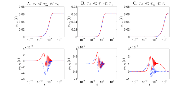
Fig. 4: Evolution of populations and coherences of an underdamped V-system ($\frac{\Delta_{p}}{\bar{\gamma}}\gg 1$) evaluated with aligned transition dipole moments ($p=1$). Here $\gamma_{1}=1.0=\gamma_{2}=\gamma$ and $\Delta=24.0$. Three different turn on regimes are shown here. Panels A show the ultrafast turn on of the field with $\tau_{r}=0.024\tau_{\Delta}$ while Panels B and C show the intermediate ($\alpha=24\tau_{\Delta}$) and slow ($\alpha=100\tau_{\gamma}$) turn on regimes respectively. Note the difference in y-axis scales for the coherence plots. Solid red lines indicate the real part of the coherence $\rho_{e_{1}e_{2}}^{R}$ with the imaginary part $\rho_{e_{1}e_{2}}^{I}$ indicated by the dashed blue line.

Equation 39c is cumbersome and does not provide much insight into the dynamics of the system. However, we note that the steady state of the system can easily be determined to be the incoherent mixture $\lim_{t\to\infty}\bm{x}(t)=[\bar{n},\bar{n},0,0]$. This agrees with the results from both the overdamped regime and the stationary field case Dodin et al. (2016). In order to obtain more insight into the dynamics of the V-system we consider several cases for the turn on time.

First, consider a turn on time, $\tau_{r}=\alpha^{-1}$, that is faster than all three of the system timescales, $\tau_{\gamma_{i}}=1/\gamma_{i}$ and the period of coherence oscillations $\tau_{\Delta}=1/\Delta_{p}$, i.e., the fast turn on regime characterized by, $\tau_{r}\ll\tau_{\Delta}\ll\tau_{\gamma_{i}}$. A binomial expansion of Eq. 39c yields the dynamics induced by a bath with a fast turn on as:

$$\rho_{e_{i},e_{i}}(t)=\bar{n}(1-e^{-\gamma_{i}t})$$ (40a)

$$\rho_{e_{1},e_{2}}^{R}(t)=\frac{p\sqrt{r_{1}r_{2}}}{\Delta_{p}}e^{-\bar{\gamma}t}\sin(\Delta_{p}t)$$ (40b)

$$\rho_{e_{1},e_{2}}^{I}(t)=\frac{p\sqrt{r_{1}r_{2}}}{\Delta_{p}}\left(e^{-\bar{\gamma}t}(\cos(\Delta_{p}t)-1)-\frac{e^{-\gamma_{1}t}-e^{-\gamma_{2}t}}{2}\right)$$ (40c)

As expected, this is identical to the solution derived for stationary fields Dodin et al. (2016). That is, if the field is turned on much faster than the characteristic timescales of the system, the stationary field solution closely approximates the evolution of the system since the field reaches its stationary state faster than the system can evolve under the transient field.

In contrast, consider a field that turns on much slower than the period of coherence oscillations, $\tau_{r}\gg\tau_{\Delta}$. In the $\tau_{\Delta}\ll\tau_{r}$ limit Eq. 39b for the real part of the coherence term takes on the much simpler form:

$$\rho_{e_{1}e_{2}}^{R}(t)=\frac{p\sqrt{r_{1}r_{2}}}{\Delta_{p}}\frac{\alpha}{\Delta_{p}}(e^{-\bar{\gamma}t}\cos(\Delta_{p}t)-e^{-\alpha t})$$ (41)

which does not depend on the value of $\tau_{r}$ relative to $\tau_{\gamma_{i}}$. Equations 39a and 39c for the populations and the imaginary part of the coherence term depend on the magnitude of $\tau_{r}$ relative to each of the $\tau_{\gamma_{i}}$’s. Equation 40a remains an accurate solution for $\rho_{e_{i}e_{i}}(t)$ provided that $\tau_{\gamma_{i}}\gg\tau_{r}$. In the adiabatic ($\tau_{\gamma_{i}}\ll\tau_{r}$) limit, the populations can be expressed as

$$\rho_{e_{i}e_{i}}(t)=\bar{n}(1-e^{-\alpha t})=\bar{n}(t)$$ (42)

Equation 40c remains a good approximation for the imaginary coherences provided that $\tau_{r}\ll\tau_{\gamma_{i}}$. More generally, $\rho_{e_{1}e_{2}}^{I}(t)$ depends on the magnitude of $\tau_{r}$ relative to both $\tau_{\gamma_{i}}$’s. Without loss of generality, let $\gamma_{1}>\gamma_{2}$. This gives the dynamics of the imaginary coherences in the following cases:

Significantly, in the adiabatic limit, when the turn on time of the field far exceeds the characteristic timescales of the system, the coherences in Eqs. 43 and 41 are heavily suppressed by the factor of $\frac{\tau_{\Delta}}{\tau_{r}}\ll 1$ relative to the fast turn on case Eqs. 40b and 40c. Therefore, the V-system is in equilibrium with the field at all times in the adiabatic limit, producing an incoherent mixture of excited states at all times.

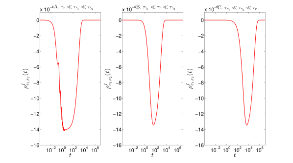
Fig. 5: Evolution of the imaginary coherences of an underdamped V-system ($\frac{\Delta_{p}}{\bar{\gamma}}\gg 1$) evaluated with aligned transition dipole moments ($p=1$). Here $\gamma_{1}=2.0$, $\gamma_{2}=10^{-3}$ and $\Delta=24.0$. Three different turn on regimes are shown here. Panels A shows the ultrafast turn on of the field with $\tau_{r}=2\times 10^{-3}\tau_{\gamma_{1}}$ while Panels B and C show the intermediate ($\tau_{r}=20\tau_{\gamma_{1}}=0.01\tau_{\gamma_{2}}$) and slow ($\tau_{r}=100\tau_{\gamma_{2}}$) turn on regimes respectively. Note the difference in y-axis scales for the coherence plots.

The rich dynamics of the imaginary coherences, $\rho_{e_{1}e_{2}}^{I}$, are hidden in Fig. 4 due to the assumption of equal decay rates. Figure 5 displays the interplay between the oscillatory and quasistationary contributions more clearly by selecting highly asymmetric decay widths $\gamma_{1}\gg\gamma_{2}$.

Furthermore, Eqs. 34b, 41 and 43 all display the same inverse scaling of coherence amplitude with turn on time of the field. Hence, if a radiation field is turned on slowly, the magnitude of the coherences scales inversely with the turn on time as

$$\max\{|\rho_{e_{1}e_{2}}|(t)\}\propto\alpha=\frac{1}{\tau_{r}}$$ (44)

This suggests that the strong coherences observed thus far Tscherbul and Brumer (2014a); Dodin et al. (2016) for $\Delta\neq 0$ arise due to the instantaneous turn on of the radiation field and will not be retained when considering a field with a turn on time that is slower than the radiative lifetimes of the excited states ($\tau_{r}\gg\tau_{\gamma_{i}}=1/\gamma_{i}$).

In summary, in both the overdamped and underdamped regions, the Fano coherences previously computed in the study of V-systems with suddenly turned-on radiation Tscherbul and Brumer (2015, 2014a); Dodin et al. (2016) disappear if the incoherent radiation field is turned on adiabatically. Similarly, these results clearly indicate that coherences observed in experiments utilizing fast laser pulses (e.g. Collini et al. (2010); Engel et al. (2007)) will not appear in nature where turn on times are essentially infinite on molecular time scales. Some explicit cases are discussed in Sec. VII below.

VII Sample Light Harvesting Cases

The above results encompass a vast range of possible systems. It is advantageous, therefore, to focus on some simple cases to emphasize the importance of these results to molecules of interest in, e.g., light harvesting scenarios. We address two sample questions below, being generous in our requirements for coherences. Note that we assume below that the system is isolated from an external (e.g. protein) environment, so as to focus solely on relaxation effects due to the incoherent light. This artificial arrangement is only designed to highlight some of the timescales associated with the above analysis.

(i) Light-induced coherences have been observed experimentally in FMO, PC645 and other light harvesting complexes Tiwari et al. (2013); Collini et al. (2010); Engel et al. (2007). In these cases $\Delta\sim 100$ cm^-1 and $\gamma$, due to spontaneous emission, is on the order of $1$ ns^-1, which places the system in the overdamped region. For the sake of simplicity, this discussion neglects non-radiative relaxation and decay of the excited states due to the interaction with the phonons, which play an important role in realistic models of light-harvesting complexes Tscherbul and Brumer .

Given our results above we can ask, for example: what turn-on time scales would be required to produce coherences that are even a modest $1\%$ of the population? Using Eq. 41 shows that $|\rho_{e_{1}e_{2}}|/\rho_{e_{i}e_{i}}=\gamma/(\Delta_{p}^{2}\tau_{r})$. Hence, the turn-on time must be faster than $\sim 10-100$ ns, clearly far faster than natural turn-on times. Hence, these coherences will not occur in natural light-harvesting systems.

(ii) Alternatively, we might ask what coherences (that are a modest $1\%$ of the population) can be generated by a turn-on time of $1$ ms, still a relatively fast turn-on time on natural time scales.

Here, using the same approach, we have $|\rho_{e_{1}e_{2}}|/\rho_{e_{i}e_{i}}=\gamma/(\Delta_{p}^{2}\tau_{r})$. Requiring this ratio to be a modest $1\%$ shows that states that will display coherences are separated by less than $0.9$ cm^-1. Analogously, if we utilize a more realistic turn-on time of 1s, only levels separated by $9\times 10^{-4}$ cm^-1 will display coherences. Once again, the results highlight the significance of the slow turn-on to assessing the (lack of) involvement of coherent phenomena in natural cases.

VIII Conclusion

We have presented a generalization of the Bloch-Redfield master equations to the case of time-varying radiation fields. They are shown to be of a similar structure to the previously studied master equations for stationary fields Tscherbul and Brumer (2015, 2014a); Dodin et al. (2016), but with time-dependent incoherent pumping rates $r_{i}(t)$. We explicitly determined the form of these master equations for the class of three-level V-systems and solved them analytically in the weak pumping limit relevant to the natural incident light (e.g. solar radiation).

Following the approach taken in the study of V-systems interacting with stationary fields Dodin et al. (2016); Tscherbul and Brumer (2014a) two limiting cases were considered in detail. The underdamped regime ($\Delta_{p}\gg\bar{\gamma}$) characterized by oscillatory coherences and the overdamped regime ($\bar{\gamma}\gg\Delta_{p}$) characterized by quasistationary coherences. In both regimes an inverse relationship between the maximal magnitude of the coherences and the turn on time $\max\{|\rho_{e_{1}e_{2}}|\}\propto 1/\tau_{r}$ in the adiabatic limit of very slow field turn-on was established. This corresponds to a V-system in equilibrium with the radiation field at all times. In other words, the system is always approximately in the equilibrium mixture $\rho_{eq}=[\bar{n}(t),\bar{n}(t),0,0]^{T}$.

By contrast, for the very fast turn on of the radiation field, both regimes show dynamics that are identical to the sudden turn-on of the radiation field studied in the stationary field case ($\tau_{r}\to 0$). This limit occurs when the turn on time is much faster than any of the system timescales, so that the system does not evolve under the transient field. Instead it evolves under the steady state field that is reached very quickly.

For intermediate turn on times, the dynamics of the system can vary from those observed in the stationary field case but they, in general, reach the same maximal coherence as in the sudden turn on case. One unexpected phenomenon observed was the synchronized decay of the coherences where all coherent superpositions decayed at the same time. This differs from the naive expectation that coherent superpositions produced at later times would decay later than those produced at earlier times. This synchronized decay of coherent superpositions occurs due to the suppression of excited state coherences by excited state populations. When the coherences produced at early times decay, they lead to an increased population of the excited state manifold. This subsequently leads to an increase in the decay rate of the coherent superpositions, which leads to a further increase in the excited state population. Ultimately, this process leads to the run-away increase of the decay rate of the coherences at the decay time of the first superpositions prepared by the incident field and hence the synchronized decay of coherences.

These results reveal nontrivial effects of the turn on rate of the incoherent field on the dynamics of the system. Most significantly they suggest that the significant coherences observed in the study of the V-system do not survive the slow turn-on of the radiation field. Moreover, in the isolated molecule case, they will not survive for a field with a turn on time slower than the radiative lifetime of the excited states $\tau_{\gamma_{i}}=1/\gamma_{i}$ for a V-system in the underdamped limit or slower than the long time scale $\tau_{\Delta}=2\bar{\gamma}/\Delta_{p}^{2}$ in the overdamped limit. This greatly restricts the class of systems that would display significant coherences for radiation fields with physical turn-on times.

The implication of these results for pulsed laser experiments Engel et al. (2007); Collini et al. (2010); Chenu and Scholes (2015) that display coherences in biological molecules is profound. Specifically, they imply that illumination by natural sunlight, where turn-on times are indeed enormously longer than all other relevant dynamical time scales, can not generate Fano coherences between other than essentially degenerate states.

Acknowledgements

This work was supported by the US AFOSR through Contract No. FA9550-13-1-0005, and by NSERC.

Appendix A Generality of Results

To prove the generality of the results for the exponential turn on function Eq. 5 presented in the main text, consider the set, $S$, of all continuous driving functions, $\bar{n}(t)$, such that the function is initially zero and evolves to a steady state value, $\bar{n}$, in the long time limit. That is

$$S=\left\{\bar{n}(t):[0,\infty)\to\mathbb{R}\;|\>\bar{n}(t)\in C_{1};\;\bar{n}(0)=0;\;\lim_{t\to\infty}\bar{n}(t)=\bar{n}\right\}$$ (45)

An element of $S$ in Eq. 45 can, in general, be written as

$$\bar{n}(t)=\bar{n}-{g}(t)$$ (46)

where $g(t)\in C_{0}([0,\infty),\mathbb{R})$ and $C_{0}([0,\infty),\mathbb{R})$ is the set of continuous functions from the interval $[0,\infty)$ on the real line to $\mathbb{R}$ which vanish at infinity.

We proceed now to prove that any function $g(t)\in C_{0}([0,\infty),\mathbb{R})$ can be written as a series of decaying exponentials on the positive real half-line. This can be done using the Stone-Weierstrass theorem on locally compact spaces Willard (2004). A set of functions, $A$, on $X$ is said to vanish nowhere if, for any $x\in X$, there exists a function, $f\in A$ such that $f(x)\neq 0$. It is said to separate points if $\forall x\neq y\in X$ there exists a function $g\in A$ such that $g(x)\neq g(y)$. Further, $C_{0}(X,\mathbb{R})$ defines an algebra over $\mathbb{R}$ under pointwise addition and multiplication of functions.

Theorem 1.

(Stone-Weierstrass) Suppose $X$ is a locally compact Hausdorff space and $A$ is a subalgebra of $C_{0}(X,\mathbb{R})$. Then $A$ is dense in $C_{0}(X,\mathbb{R})$ if and only if it separates points and vanishes nowhere.

Begin by considering the interval $X=[0,\infty)$. This is a closed subset of the locally compact Hausdorff space $\mathbb{R}$ and so is itself a locally compact Hausdorff space. Define A as follows

$$A=span\{h_{a}(t)=e^{-at}|a\in\mathbb{R}_{+};\;t\in[0,\infty)\}$$ (47)

where $\mathbb{R}_{+}$ is the set of positive real numbers. Clearly $A$ defines a vector space over the real numbers under pointwise addition and scalar multiplication of functions. Furthermore, all decaying exponentials vanish at infinity so $A$ is contained in $C_{0}([0.\infty),\mathbb{R})$. The product of linear combinations of decaying exponentials produces another such linear combination of exponentials, guaranteeing closure of $A$ under pointwise multiplication. Therefore $A$ defines a subalgebra of $C_{0}([0,\infty),\mathbb{R})$. It is trivial to show that $A$ vanishes nowhere and separates points on $[0,\infty)$.

Hence, according to this theorem, $A$ is dense in $C_{0}([0,\infty),\mathbb{R})$. By the definition of a dense space, any function $g(t)\in C_{0}([0,\infty),\mathbb{R})$ is either in $A$ or is a limit point of $A$ Steen and Seebach (1995). In other words, any function, $g(t)$, vanishing at infinity on the positive real half-line can be expressed in the following form:

$$g(t)=\int_{0}^{\infty}daf(a)e^{-at}=-\left(\int_{0}^{\infty}daf(a)(1-e^{-at})\right)+\int^{\infty}_{0}daf(a)$$ (48)

Substituting Eq. 48 into Eq. 46, and applying the initial condition $\bar{n}(0)=0$ yields the constraint $\bar{n}=\int^{\infty}_{0}daf(a)$. This allows Eq. 46 to be rewritten as

$$\bar{n}(t)=\int^{\infty}_{0}daf(a)(1-e^{-at})$$ (49)

Equation 49 expresses a general class of driving function as a series of terms each of the form considered in the main text Eq. 5. The integral transform in Eq. 48 is very similar to a Laplace Transform with the transformed coordinate, $a$, restricted to the real line rather than the complex plane Boyce and DiPrima (2009). This yields an intuitive expansion of the time-dependent occupation number Eq. 49 in a basis where each basis function ($f_{\alpha}(t)=1-e^{-\alpha t}$) is associated with a characteristic turn on time $\tau_{\alpha}=1/\alpha$.

Using Eq. 49, the driving vector $\bm{d}(t)$ in Eq. 25c for an arbitrary driving function is given by

$$\bm{d}(t)=\left(\begin{array}[]{c}\gamma_{1}\\ \gamma_{2}\\ p\sqrt{\gamma_{1}\gamma_{2}(t)}\\ 0\end{array}\right)\int^{\infty}_{0}daf(a)(1-e^{-at})=\mathbf{d}\int^{\infty}_{0}daf(a)(1-e^{-at})$$ (50)

Substituting Eq. 50 into the general variation of parameters solution Eq. 28 yields the solution for an arbitrary turn on function in terms of the solutions derived in the text.

$$\bm{x}(t)=\int^{\infty}_{0}daf(a)\int^{t}_{0}dse^{A^{(0)}(t-s)}\mathbf{d}(1-e^{-at})=\int^{\infty}_{0}daf(a)\bm{x_{a}}(t)$$ (51)

where $\bm{x_{a}}(t)$ is the solution for a turn on function $\bar{n}_{a}(t)=(1-e^{-at})$.

Equation 51 applied to the coherences indicates that any coherences observed are a result of the components with a fast turn on time.

References

- Tiwari et al. (2013) V. Tiwari, W. K. Peters, and D. M. Jonas, Proc. Natl. Acad. Sci. USA 110, 1203 (2013).
- Collini et al. (2010) E. Collini, C. Y. Wong, K. E. Wilk, P. M. G. Curmi, P. Brumer, and G. D. Scholes, Nature (London) 463, 644 (2010).
- Engel et al. (2007) G. S. Engel, T. R. Calhoun, E. L. Read, T.-K. Ahn, T. Mančal, Y.-C. Cheng, R. E. Blankenship, and G. R. Fleming, Nature (London) 446, 782 (2007).
- Hau et al. (1999) L. V. Hau, S. E. Harris, Z. Dutton, and C. H. Behroozi, Nature (London) 397, 594 (1999).
- Grinev and Brumer (2015) T. Grinev and P. Brumer, J. Chem. Phys. 143, 244313 (2015).
- Tscherbul and Brumer (2015) T. V. Tscherbul and P. Brumer, J. Chem. Phys. 142, 104107 (2015).
- Chenu et al. (2015) A. Chenu, A. M. Brańczyk, G. D. Scholes, and J. Sipe, Phys. Rev. Lett. 114, 213601 (2015).
- Tscherbul and Brumer (2014a) T. V. Tscherbul and P. Brumer, Phys. Rev. Lett. 113, 113601 (2014a).
- Sadeq and Brumer (2014) Z. S. Sadeq and P. Brumer, J. Chem. Phys. 140, 074104 (2014).
- Olšina et al. (2014) J. Olšina, A. G. Dijkstra, C. Wang, and J. Cao, arXiv:1408.5385 [physics, physics:quant-ph] (2014), arXiv: 1408.5385.
- Tscherbul and Brumer (2014b) T. V. Tscherbul and P. Brumer, J. Phys. Chem. A 118, 3100 (2014b).
- Brumer and Shapiro (2012) P. Brumer and M. Shapiro, Proc. Natl. Acad. Sci. USA 109, 19575 (2012).
- Pachón and Brumer (2012) L. A. Pachón and P. Brumer, Phys. Chem. Chem. Phys. 14, 10094 (2012).
- Mančal and Valkunas (2010) T. Mančal and L. Valkunas, New J. Phys. 12, 065044 (2010).
- Ou et al. (2008) B.-Q. Ou, L.-M. Liang, and C.-Z. Li, Opt. Commun. 281, 4940 (2008).
- Agarwal and Menon (2001) G. S. Agarwal and S. Menon, Phys. Rev. A 63, 023818 (2001).
- Jiang and Brumer (1991) X.-P. Jiang and P. Brumer, J. Chem. Phys. 94, 5833 (1991).
- Dodin et al. (2016) A. Dodin, T. V. Tscherbul, and P. Brumer, J. Chem. Phys. 144, 244108 (2016).
- Cohen-Tannoudji et al. (1992) C. Cohen-Tannoudji, J. Dupont-Roc, G. Grynberg, and P. Thickstun, Atom-photon interactions: basic processes and applications (Wiley Online Library, 1992).
- Loudon (2000) R. Loudon, The Quantum Theory of Light (OUP Oxford, 2000).
- Fleischhauer et al. (1992) M. Fleischhauer, C. H. Keitel, M. O. Scully, and C. Su, Opt. Commun. 87, 109 (1992).
- Kozlov et al. (2006) V. V. Kozlov, Y. Rostovtsev, and M. O. Scully, Phys. Rev. A 74, 063829 (2006).
- Agarwal (1974) D. G. S. Agarwal, in Quantum Optics, Springer Tracts in Modern Physics No. 70 (Springer Berlin Heidelberg, 1974) pp. 1–128, dOI: 10.1007/BFb0042382.
- Kiffner et al. (2010) M. Kiffner, M. Macovei, J. Evers, and C. H. Keitel, Progress in Optics, edited by E. Wolf, Vol. 55 (North Holland, Amsterdam, 2010) sec 3.2.5.
- Dorfman et al. (2013) K. E. Dorfman, D. V. Voronine, S. Mukamel, and M. O. Scully, Proc. Natl. Acad. Sci. USA 110, 2746 (2013).
- (26) 108, 10.1073/pnas.1110234108.
- (27) T. V. Tscherbul and P. Brumer, (manuscript in preparation).
- (28) A. Dodin, T. V. Tscherbul, and P. Brumer, (Work in Progress).
- Pachón and Brumer (2013) L. A. Pachón and P. Brumer, Phys. Rev. A 87, 022106 (2013).
- Scully and Zubairy (1997) M. O. Scully and M. S. Zubairy, Quantum Optics (Cambridge University Press, 1997).
- Mandel and Wolf (1995) L. Mandel and E. Wolf, Optical Coherence and Quantum Optics (Cambridge University Press, 1995).
- Breuer and Petruccione (2007) H.-P. Breuer and F. Petruccione, The theory of open quantum systems (Oxford University Press, Oxford, 2007).
- Blum (2012) K. Blum, Density Matrix Theory and Applications (Springer Science & Business Media, 2012).
- Boyce and DiPrima (2009) W. E. Boyce and R. C. DiPrima, Elementary differential equations and boundary value problems (Wiley, Hoboken, NJ, 2009) oCLC: 302295891.
- Chenu and Scholes (2015) A. Chenu and G. D. Scholes, Annu. Rev. Phys. Chem. 66, 69 (2015).
- Willard (2004) S. Willard, General topology, Dover books on mathematics (Dover Publ, Mineola, NY, 2004) oCLC: 637239058.
- Steen and Seebach (1995) L. A. Steen and J. A. Seebach, Counterexamples in Topology (Courier Corporation, 1995).