The Rest-Frame Optical Spectroscopic Properties of Ly$\alpha$-Emitters at $Z\sim 2.5$: The Physical Origins of Strong Ly$\alpha$ Emission

Abstract

We present the rest-frame optical spectroscopic properties of 60 faint ($R_{\textrm{\scriptsize{AB}}}\sim 27$; $L\sim 0.1L_{*}$) Ly$\alpha$-selected galaxies (LAEs) at $z\approx 2.56$. These LAEs also have rest-UV spectra of their Ly$\alpha$ emission line morphologies, which trace the effects of interstellar and circumgalactic gas on the escape of Ly$\alpha$ photons. We find that the LAEs have diverse rest-optical spectra, but their average spectroscopic properties are broadly consistent with the extreme low-metallicity end of the populations of continuum-selected galaxies selected at $z\approx 2-3$. In particular, the LAEs have extremely high [O III] $\lambda$5008/H$\beta$ ratios (log([O III]/H$\beta$) $\sim$ 0.8) and low [N II] $\lambda$6585/H$\alpha$ ratios (log([N II]/H$\alpha$) $<1.15$). Coupled with a detection of the [O III] $\lambda$4364 auroral line, these measurements indicate that the star-forming regions in faint LAEs are characterized by high electron temperatures ($T_{e}\approx 1.8\times 10^{4}$K), low oxygen abundances (12 + log(O/H) $\approx$ 8.04, $Z_{\textrm{\scriptsize{neb}}}\approx 0.22Z_{\odot}$), and high excitations with respect to their more luminous continuum-selected analogs. Several of our faintest LAEs have line ratios consistent with even lower metallicities, including six with 12 + log(O/H) $\approx$ 6.9$-$7.4 ($Z_{\textrm{\scriptsize{neb}}}\approx 0.02-0.05Z_{\odot}$). We interpret these observations in light of new models of stellar evolution (including binary interactions) that have been shown to produce long-lived populations of hot, massive stars at low metallicities. We find that strong, hard ionizing continua are required to reproduce our observed line ratios, suggesting that faint galaxies are efficient producers of ionizing photons and important analogs of reionization-era galaxies. Furthermore, we investigate the physical trends accompanying Ly$\alpha$ emission across the largest current sample of combined Ly$\alpha$ and rest-optical galaxy spectroscopy, including both the 60 KBSS-Ly$\alpha$ LAEs and 368 more luminous galaxies at similar redshifts. We find that the net Ly$\alpha$ emissivity (parameterized by the Ly$\alpha$ equivalent width) is strongly correlated with nebular excitation and ionization properties and weakly correlated with dust attenuation, suggesting that metallicity plays a strong role in determining the observed properties of these galaxies by modulating their stellar spectra, nebular excitation, and dust content.

1. Introduction

The optical emission lines of galaxies can provide a wealth of information regarding the properties of young stars and the regions in which they form. The historical accessibility of optical wavelengths has enabled large spectroscopic surveys to measure these lines in local star-forming regions and thereby identify and calibrate their relationships with the physical properties of galaxies. These properties include star-formation rates, elemental abundances, gas temperatures and densities, ionization states, and the nature of sources of ionizing radiation within galaxies and gaseous clouds. In particular, the Baldwin et al. (1981) line ratios (including the N2-BPT ratios [N II]/H$\alpha$ and [O III]/H$\beta$) are frequently used to discriminate between ionization by star formation and/or active galactic nuclei (AGN), and these same line ratios provide a measure of gas-phase metallicity among star-forming galaxies (Dopita et al., 2000).

At $z\gtrsim 1$, however, these well-studied transitions shift into infrared bands, where efficient, multiplexed spectrocopic survey instruments have only recently become available (e.g., Keck/MOSFIRE [McLean et al. 2012]; VLT/KMOS [Sharples et al. 2013]). In the last few years, these spectrometers have enabled the collection of the first statistical samples of galaxies at $z\approx 2-3$ with rest-optical spectra, in particular through the Keck Baryonic Structure Survey (KBSS; Steidel et al. 2014; Strom et al. 2016) and the MOSFIRE Deep Evolution Field survey (MOSDEF; Kriek et al. 2015).

One of the earliest results of these new surveys has been that the nebular emission line ratios of high-redshift galaxies occupy a distinct locus in the N2-BPT parameter space with respect to typical low-redshift galaxies (e.g., from the Sloan Digital Sky Survey; SDSS). Earlier limited rest-optical spectroscopy had hinted at this trend (Shapley et al., 2005; Erb et al., 2006; Liu et al., 2008; Brinchmann et al., 2008), but the KBSS and MOSDEF surveys have demonstrated that the population of bright continuum-selected galaxies (LBGs; $L\sim L_{*}$) is shifted toward high [O III]/H$\beta$ ratios at fixed [N II]/H$\alpha$ (or equivalently, high [N II]/H$\alpha$ at fixed [O III]/H$\beta$) with respect to the SDSS star-forming galaxy locus (Steidel et al., 2014, 2016; Shapley et al., 2015; Sanders et al., 2015; Strom et al., 2016).

While this trend has been firmly established for LBGs, its physical origins remain under debate. Several studies have suggested that this “BPT offset” may be explained by high N/O ratios at $z\approx 2-3$ (Masters et al., 2014, 2016; Sanders et al., 2015), which would produce a shift toward high [N II]/H$\alpha$. However, Strom et al. (2016) present detailed rest-optical spectroscopy of $\sim$250 LBGs over a wide range of stellar masses and star-formation rates (SFRs), finding behavior consistent with the low-redshift N/O vs. O/H relation. Rather, Strom et al. (2016) (along with Steidel et al. 2014, 2016) suggest that the N2-BPT offset corresponds primarily to a change in the excitation state of nebular gas, which can be explained by the presence of stars with hotter, harder spectra than typical of stars in the local Universe.

At the same time, new studies of massive stars have indicated that the rotation and binarity of stars play important roles in shaping their evolution and emission (e.g., Eldridge & Stanway 2009; Brott et al. 2011; Levesque et al. 2012). These effects can cause stars to exhibit longer lifetimes and higher-temperature spectral shapes than their single or slowly-rotating counterparts. Furthermore, these effects may naturally be more pronounced at high redshifts, where low photospheric metallicities produce weaker winds and less associated loss of angular momentum. Similarly, lower-metallicity stars produce harder spectra regardless of their rotation rate, and metallicity may influence stellar binarity through the cooling and fragmentation of star-forming clouds.

In light of these trends, Steidel et al. (2016) used extremely deep composite LBG spectra in the rest-UV and rest-optical to measure a suite of emission lines and their ratios, finding that stellar spectra from the Binary Population and Spectral Synthesis (BPASSv2; Eldridge & Stanway 2016; Stanway et al. 2016) models are able to reproduce the full set of measured values. Conversely, the softer spectra of single-star models, including non-binary BPASSv2 models and those from the Starburst99 model suite (Leitherer et al., 2014), do not fulfill these constraints irrespective of the assumed N/O ratio.

In addition to these observational constraints, model spectra similar to those produced by binary evolution models are preferred by other observations as well as theoretical grounds. Most obvious is that approximately 70% of local massive stars are expected to experience mass transfer in binary systems (e.g., Sana et al. 2012), so single star models are unlikely to provide an accurate description of their evolution. Secondly, simulations of ionizing photon production have extreme difficulty generating the large escape fractions needed to reionize the Universe, in part because the stars remain buried in their optically thick birth clouds for longer than the $\lesssim$3 Myr lifetimes expected for strong sources of ionizing photons in typical stellar models (e.g., Ma et al. 2015). Models that maintain populations of hot, luminous stars for 3$-$10 Myr (including the aformentioned binary models) continue to produce ionizing photons after their birth clouds have been cleared away by stellar feedback, which allows the photons to escape to large radii. Ma et al. (2016) demonstrate that simulations from the Feedback In Realistic Environments (FIRE; Hopkins et al. 2014) project that include the BPASSv2 stellar models are able to reproduce the high escape fractions of ionizing photons required by other constraints on reionization (e.g., Robertson et al. 2015). Modeling the epoch of reionization (EoR) therefore requires further understanding of the stellar populations of these galaxies.

The specific galaxies that dominated the EoR, however, were less luminous and less mature than those selected as LBGs at $z\approx 2-3$. One method of identifying galaxies with properties more analgous to the EoR population is by selecting on the basis of Ly$\alpha$ line emission. As this technique does not require a detection in the stellar continuum, it naturally selects fainter, younger, and lower-mass galaxies than typical samples of LBGs (e.g., Gawiser et al. 2006). We have also shown through the KBSS-Ly$\alpha$ survey (Trainor et al., 2015) that these Ly$\alpha$-emitting galaxies (LAEs) have lower covering fractions of interstellar and/or circumgalactic gas, which allows a higher fraction of their UV photons to escape. Furthermore, there is evidence from radiative-transfer simulations that the physical conditions which facilitate Ly$\alpha$ emission are also conducive to ionizing photon escape (Dijkstra et al. 2016, but cf. Yajima et al. 2014).

LAEs comprise an increasing proportion of galaxies as redshift increases up to the EoR at $z\approx 6$ (e.g., Stark et al. 2010, 2011), above which the fraction drops due to Ly$\alpha$ absorption and scattering by the neutral intergalatic medium (Pentericci et al., 2011; Schenker et al., 2012; Ono et al., 2012). However, the intrinsic Ly$\alpha$ emissivity of galaxies (divorced from their intergalactic and circumgalactic attenuation) likely continues to increase toward the earliest cosmic times, given the trends of Ly$\alpha$ equivalent width with galaxy luminosity and UV spectral slope (e.g., Schenker et al. 2014). For all of these reasons, LAEs at $z\approx 2-3$ are an ideal laboratory for probing the physical properties of star-formation in EoR analogs.

In addition, Strom et al. (2016) find that the high-redshift LBGs most offset from the SDSS N2-BPT locus are those with below-average masses and high specific star formation rates, indicating that low-mass LAEs provide key probes of the changing nebular conditions and stellar populations at high redshifts as well. Some previous studies of Ly$\alpha$-emitting galaxies have affirmed this interpretation: McLinden et al. (2011) measured strong [O III] emission in two LAEs at $z\approx 3.1$, Finkelstein et al. (2011) found strong [O III]/H$\beta$ and weak [N II]/H$\alpha$ in two LAEs at $z\approx 2.4$, and Nakajima et al. (2013) measured high [O III]/[O II] ratios in two LAEs and in a composite spectrum of four additional LAEs at $z\approx 2.2$. Song et al. (2014) present a sample of 16 LAEs, including 10 with rest-frame optical spectroscopy, which show similarly extreme line ratios consistent with low gas-phase and stellar metallicities. However, the relatively small sample sizes of these studies have made it difficult to establish the average properties of high-redshift LAEs. Furthermore, the LAEs in these studies have luminosities similar to those of typical LBG samples ($\sim$10$\times$ that of the KBSS-Ly$\alpha$ LAEs), which eliminates many of the advantages of continuum-faint LAEs for selecting EoR analogs.

Galaxy selections based on emission lines other than Ly$\alpha$ have also yielded similar populations. Hagen et al. (2016) find that optical-emission-line-selected galaxies exhibit a wide range of properties consistent with LAEs (although cf. Oteo et al. 2015, who find that H$\alpha$-selected galaxies are more massive and redder than LAEs). Maseda et al. (2014) present 22 Extreme Emission-Line Galaxies (EELGs) selected by H$\alpha$ or [O III] emission in grism spectroscopy, which show high excitations (log([O III]/H$\beta$) $\approx 0.7$) and low metallicities ($Z_{\textrm{\scriptsize{neb}}}=0.05-0.3Z_{\odot}$). Masters et al. (2014) present a similar grism-selected sample of 26 galaxies with a comparable N2-BPT offset to the LBG samples discussed above. Both of these EELG samples lie at slightly lower redshifts ($z\approx 1.3-2.3$) than the KBSS, KBSS-Ly$\alpha$, and MOSDEF galaxies. The EELGs also have atypically high specific star-formation rates (sSFR), with stellar and dynamical masses similar or slightly higher than those of KBSS-Ly$\alpha$ LAEs ($M_{\textrm{\scriptsize{dyn}}}\sim 10^{9}$$\rm M_{\odot}$) and SFRs 3$-$10$\times$ higher, similar to typical LBGs (SFR $\sim$ 30 $\rm M_{\odot}$ yr^-1). Most of these EELGs also do not have Ly$\alpha$ measurements (being observationally difficult at $z\lesssim 2$), which prohibits the comparison of nebular properties with Ly$\alpha$ production and escape.

This paper, therefore, has two primary objectives: 1) to extend our understanding of the nebular properties of galaxies toward low stellar masses and faint luminosities by measuring the rest-frame optical spectra of typical LAEs; and 2) to determine how the Ly$\alpha$ emissivities of galaxies are related to the physical properties of their stellar populations and star-forming regions. Toward this aim, we present deep nebular emission line spectra of 60 LAEs from the KBSS-Ly$\alpha$ sample presented in Trainor et al. (2015), as well as a comparison sample of 368 LBG spectra from the KBSS (Steidel et al., 2014; Strom et al., 2016), and rest-UV spectra covering the Ly$\alpha$ transition of each galaxy.

In Sec. 2, we describe the rest-optical LAE spectra presented in this paper, as well as the LBG spectra and rest-UV LAE spectra originally presented in previous work. Sec. 3 describes our emission line measurements from the individual object spectra and the creation and fitting of composite LAE spectra. In Sec. 4, we present diagnostic line ratios including the N2-BPT diagram in order to compare the nebular LAE properties to those of the LBG sample. In Sec. 5, we discuss the variation of Ly$\alpha$ equivalent width across the combined sample of LAEs and LBGs to infer the relationship between Ly$\alpha$ emission (and absorption) and physical galaxy properties including dust content and nebular excitation. Sec. 6 includes our photoionization modeling of the rest-optical line ratios and the resulting constraints on the properties of the gas and stellar populations (including binary star models) in the LAE star-forming regions. Finally, we provide additional physical interpretation of our results in comparison with previous work in Sec. 7 and a summary and conclusions in Sec. 8. Because the majority of our observed properties are line ratios, our results have little dependence on the assumed cosmology, but we assume a $\Lambda$CDM universe with ($\Omega_{m}$, $\Omega_{\Lambda}$, $H_{0}$) = (0.3, 0.7, 70 km s^-1 Mpc^-1) when necessary.

2. Observations

2.1. LAE sample

LAEs were selected from the KBSS-Ly$\alpha$ (Trainor et al. 2015; hereafter T15) sample of LAEs. The KBSS-Ly$\alpha$ is a survey for Ly$\alpha$-emitting objects in the Keck Baryonic Structure Survey (KBSS; Rudie et al. 2012; Steidel et al. 2014; Strom et al. 2016) fields, which are centered on hyperluminous QSOs at $z\sim 2-3$. The spectroscopic properties of the KBSS-Ly$\alpha$ LAE sample are described in detail in T15 and Trainor & Steidel (2013), and the full photometric parent sample of objects will be described in an upcoming paper (R. Trainor et al., in prep.). Briefly, the LAEs are selected via imaging in narrowband filters selecting Ly$\alpha$ emission near the redshift of the QSO in each KBSS field. These narrowband images are combined with deep continuum images to isolate objects with strong Ly$\alpha$ emission, typically defined as a rest-frame photometric equivalent width $W_{\textrm{\scriptsize{Ly$\alpha$}}}>20$Å. The selected objects have a limiting narrowband magnitude $m_{\textrm{\scriptsize{NB,AB}}}=26.5$, corresponding to an integrated Ly$\alpha$ line flux $F_{\textrm{\scriptsize{Ly$\alpha$}}}>10^{-17}$ erg s^-1 cm^-2 for a continuum-free source, or $F_{\textrm{\scriptsize{Ly$\alpha$}}}\gtrsim 6\times 10^{-18}$ erg s^-1 cm^-2 for a typical LAE with $W_{\textrm{\scriptsize{Ly$\alpha$}}}\approx 40$Å. The LAEs have typical continuum magnitudes $\mathcal{R}_{\textrm{\scriptsize{AB}}}(6930$Å$)\approx 27$, corresponding to $L\sim 0.1L_{*}$ at $z\sim 2.6$ from the luminosity functions of Reddy et al. (2008). As discussed in T15, the primary contaminants to the sample (as estimated by rest-UV spectroscopy of the putative Ly$\alpha$ line and surrounding wavelengths) are low-redshift [O II] emitters or intermediate-redshift AGN with high equivalent width C IV $\lambda\lambda$1549,1551 or He II $\lambda$1640 line emission, and the estimated contamination rate of the photometric sample is 3%. Given that all the LAEs and LBGs presented in this paper have multiple spectroscopic line detections, we expect that there are no such contaminants in this sample.

The properties of the individual LAEs presented in this paper are summarized in Table 1. The majority of the LAEs lie in the Q2343 field ($z_{\textrm{\scriptsize{QSO}}}=2.573$) of T15, with the remainder selected from a new field (Q1603) centered on the hyperluminous QSO HS1603+3820 ($z_{\textrm{\scriptsize{QSO}}}=2.551$). Because this QSO lies at a very similar redshift to the Q2343 QSO, the Q1603 LAEs were selected with the same NB4325 filter used for the Q2343 field, as described in T15. Properties of HS1603+3820 and its surrounding field are presented in Trainor & Steidel (2012). This field has slightly shallower narrowband imaging (by $\sim$0.5 mag) than the other KBSS-Ly$\alpha$ fields, resulting in a limiting Ly$\alpha$ luminosity $\sim$60% higher, but the properties of the Q1603 LAEs appear to be otherwise consistent with the remainder of the KBSS-Ly$\alpha$ sample.

As discussed in T15, the KBSS-Ly$\alpha$ LAEs have typical dynamical masses $\langle M_{\textrm{\scriptsize{dyn}}}\rangle\approx 8\times 10^{8}$ $\rm M_{\odot}$, and our measurements of stacked LAE spectral energy distributions (SEDs; R. Trainor et al., in prep.) imply stellar masses $M_{*}\sim 10^{8}-10^{9}$ $\rm M_{\odot}$.

Table 1MOSFIRE LAE Properties

Object Name	$z_{\textrm{\scriptsize{sys}}}$	RA	Dec	+$\mathcal{R}$	$W_{\textrm{\scriptsize{Ly$\alpha$}}}$	Bands	[O III] $\lambda$5008	H$\beta$
Q1603-NB1036	2.5412	16:04:43.35	+38:11:16.47	$>$27.3	058.8	H	20.6$\pm$2.10	2.2$\pm$1.8
Q1603-NB1365	2.5491	16:04:54.62	+38:14:01.55	+25.0	084.4	H	54.6$\pm$2.10	9.0$\pm$1.7
Q1603-NB1599	2.5471	16:04:54.89	+38:13:11.81	$>$27.3	107.7	H	46.4$\pm$2.00	$<$10.9
Q1603-NB1700	2.5447	16:04:57.60	+38:12:25.04	+24.7	053.0	H	69.6$\pm$3.60	14.2$\pm$3.70
Q1603-NB1756	2.5541	16:05:03.28	+38:12:54.03	+27.1	100.9	H	17.6$\pm$1.60	7.7$\pm$4.3
Q1603-NB1934	2.5504	16:04:48.08	+38:12:09.42	+25.0	020.3	H	79.6$\pm$3.10	18.4$\pm$1.80
Q1603-NB1962	2.5514	16:04:48.79	+38:12:29.30	+25.8	079.4	H	60.8$\pm$2.50	10.3$\pm$1.70
Q1603-NB2182	2.5602	16:04:54.51	+38:12:01.08	+24.4	005.9	H	11.7$\pm$3.00	$<$1.8
Q2343-NB0193	2.5791	23:46:23.98	+12:45:52.31	+25.6	030.9	H	13.6$\pm$0.50	2.7$\pm$0.5
Q2343-NB0280	2.5777	23:46:20.67	+12:46:19.82	+26.3	052.6	H	6.0$\pm$0.7	2.0$\pm$0.5
Q2343-NB0308	2.5663	23:46:17.83	+12:46:41.53	$>$27.3	058.8	H+K	20.2$\pm$5.8	1.6$\pm$1.1
Q2343-NB0320	2.5817	23:46:17.52	+12:46:45.78	+25.4	025.4	H	19.7$\pm$2.1	5.8$\pm$0.9
Q2343-NB0345	2.5879	23:46:13.94	+12:47:11.73	+24.5	036.9	H+K	79.5$\pm$1.7	13.4$\pm$1.10
Q2343-NB0405	2.5866	23:46:22.51	+12:46:19.06	+27.0	134.8	H+K	09.2$\pm$1.5	$<$0.3
Q2343-NB0508	2.5602	23:46:32.73	+12:45:33.09	$>$27.3	156.6	H	9.6$\pm$0.9	1.2$\pm$0.4
Q2343-NB0565	2.5634	23:46:14.01	+12:47:35.29	$>$27.3	313.9	H+K	20.5$\pm$1.30	$<$1.5
Q2343-NB0585	2.5451	23:46:31.42	+12:45:47.79	$>$27.3	046.7	H	25.0$\pm$0.40	4.2$\pm$0.5
Q2343-NB0791	2.5742	23:46:33.99	+12:50:28.08	+25.7	037.4	H+K	25.8$\pm$0.60	9.9$\pm$0.9
Q2343-NB0970	2.5609	23:46:33.43	+12:50:12.93	$>$27.3	044.1	H	8.2$\pm$1.2	1.5$\pm$0.8
Q2343-NB1075	2.5610	23:46:33.23	+12:50:04.84	$>$27.3	023.7	H	2.4$\pm$0.8	0.6$\pm$0.5
Q2343-NB1093	2.5610	23:46:36.75	+12:49:40.93	$>$27.3	054.9	H	6.5$\pm$1.3	0.9$\pm$0.8
Q2343-NB1154	2.5763	23:46:26.23	+12:50:38.86	+23.7	054.1	H+K	5.9$\pm$0.4	$<$1.0
Q2343-NB1174	2.5476	23:46:24.14	+12:50:49.14	+25.0	236.6	H+K	39.6$\pm$0.70	6.0$\pm$1.6
Q2343-NB1264	2.5475	23:46:27.33	+12:50:18.73	+25.8	108.2	H	18.8$\pm$0.50	4.8$\pm$1.7
Q2343-NB1361	2.5590	23:46:34.09	+12:48:03.47	$>$27.3	090.6	H+K	10.1$\pm$1.70	1.6$\pm$1.0
Q2343-NB1386	2.5654	23:46:36.23	+12:47:46.48	$>$27.3	025.8	H+K	9.9$\pm$1.3	$<$0.9
Q2343-NB1396	2.5817	23:46:27.44	+12:48:39.87	+25.3	067.7	H	9.8$\pm$1.0	$<$1.0
Q2343-NB1416	2.5590	23:46:34.04	+12:47:57.04	$>$27.3	020.7	H+K	3.7$\pm$1.1	0.7$\pm$0.6
Q2343-NB1501	2.5590	23:46:37.77	+12:47:24.28	+27.1	035.2	H+K	21.9$\pm$1.40	2.4$\pm$0.8
Q2343-NB1518	2.5860	23:46:40.75	+12:47:02.10	+26.2	022.3	K	$-$	$-$
Q2343-NB1585	2.5648	23:46:35.59	+12:47:28.53	$>$27.3	303.4	H+K	10.3$\pm$0.90	1.8$\pm$0.8
Q2343-NB1591	2.5438	23:46:32.56	+12:47:47.05	$>$27.3	088.8	H	4.2$\pm$0.4	2.1$\pm$0.6
Q2343-NB1680	2.5795	23:46:12.50	+12:49:45.07	+26.0	043.5	H	5.7$\pm$0.5	1.2$\pm$0.6
Q2343-NB1684	2.5807	23:46:18.98	+12:49:03.47	+26.9	024.0	H	4.0$\pm$0.7	0.9$\pm$0.6
Q2343-NB1692	2.5604	23:46:39.30	+12:46:54.50	+26.8	359.2	H+K	17.6$\pm$1.50	2.2$\pm$0.8
Q2343-NB1783	2.5767	23:46:28.71	+12:47:51.04	+26.6	035.0	H+K	29.9$\pm$1.00	4.4$\pm$1.1
Q2343-NB1789	2.5450	23:46:29.21	+12:47:48.05	$>$27.3	088.2	H+K	15.1$\pm$0.50	3.8$\pm$0.5
Q2343-NB1806	2.5954	23:46:20.09	+12:48:43.60	+26.8	019.3	K	$-$	$-$
Q2343-NB1828	2.5727	23:46:25.25	+12:48:08.61	+25.8	026.7	H+K	21.7$\pm$0.50	3.5$\pm$0.4
Q2343-NB1829	2.5754	23:46:25.12	+12:48:07.80	+25.6	032.1	H+K	35.0$\pm$0.80	$<$5.5
Q2343-NB1922	2.5653	23:46:12.61	+12:49:17.22	$>$27.3	142.3	H	8.2$\pm$1.1	$<$0.7
Q2343-NB2098	2.5647	23:46:12.35	+12:49:10.62	$>$27.3	256.0	H	5.2$\pm$1.3	3.3$\pm$1.3
Q2343-NB2211	2.5756	23:46:22.90	+12:47:43.45	$>$27.3	066.2	H+K	24.6$\pm$0.60	11.7$\pm$3.70
Q2343-NB2571	2.5791	23:46:23.29	+12:46:58.64	$>$27.3	029.4	H+K	3.7$\pm$0.6	$<$1.0
Q2343-NB2785	2.5785	23:46:31.59	+12:49:31.38	$>$27.3	014.2	K	$-$	$-$
Q2343-NB2807	2.5446	23:46:40.22	+12:48:27.64	+23.4	024.6	H	143.4$\pm$9.10	45.2$\pm$4.20
Q2343-NB2816	2.5770	23:46:27.44	+12:49:53.12	$>$27.3	058.5	H+K	4.7$\pm$0.6	2.5$\pm$0.7
Q2343-NB2821	2.5753	23:46:20.59	+12:50:24.94	+27.1	032.4	H+K	6.6$\pm$0.7	$<$3.4
Q2343-NB2834	2.5683	23:46:37.77	+12:48:44.48	$>$27.3	007.2	K	$-$	$-$
Q2343-NB2835	2.5738	23:46:33.80	+12:49:10.63	$>$27.3	061.3	H	3.9$\pm$0.6	3.7$\pm$0.8
Q2343-NB2875	2.5450	23:46:33.06	+12:49:11.19	$>$27.3	287.2	H	5.6$\pm$0.5	3.3$\pm$0.5
Q2343-NB2929	2.5456	23:46:33.03	+12:49:00.27	+26.5	023.7	H	13.4$\pm$0.60	3.6$\pm$0.9
Q2343-NB2957	2.5768	23:46:37.05	+12:47:47.85	$>$27.3	023.3	H	3.4$\pm$0.4	1.4$\pm$0.4
Q2343-NB3061	2.5765	23:46:21.30	+12:50:03.51	+27.2	057.6	H+K	12.5$\pm$0.50	2.4$\pm$0.7
Q2343-NB3122	2.5648	23:46:19.50	+12:50:12.91	+26.9	080.4	H	43.2$\pm$1.20	4.3$\pm$1.2
Q2343-NB3157	2.5445	23:46:39.46	+12:48:01.31	+25.0	021.9	H	95.3$\pm$0.70	17.2$\pm$0.80
Q2343-NB3170	2.5475	23:46:39.81	+12:47:50.11	$>$27.3	090.0	H	12.0$\pm$0.60	2.9$\pm$2.3
Q2343-NB3231	2.5713	23:46:24.76	+12:49:24.97	$>$27.3	110.4	H+K	27.6$\pm$0.80	5.2$\pm$0.4
Q2343-NB3252	2.5709	23:46:31.98	+12:48:35.32	+26.1	032.9	H	10.3$\pm$1.30	1.5$\pm$0.6
Q2343-NB3292	2.5631	23:46:25.35	+12:49:09.51	$>$27.3	013.4	K	$-$	$-$

2.2. Rest-optical spectroscopic observations

Rest-frame optical spectra of the KBSS-Ly$\alpha$ LAEs were obtained using the Multi-Object Spectrometer For InfraRed Exploration (MOSFIRE; McLean et al. 2010, 2012) on the Keck 1 telescope. Initial observations (including all of the $K$-band spectroscopy presented here) were obtained over the course of the KBSS-MOSFIRE survey (Steidel et al., 2014). The data were reduced using the spectroscopic reduction pipeline provided by the instrument team, and the details of the observing strategies and reduction are described in Steidel et al. (2014). All spectra were observed using 0$\farcs$7 slits, yielding $R\approx 3660$ or $\sigma_{\textrm{\scriptsize{inst}}}\approx 35$ km s^-1.

A total of 28 LAEs were detected in the $K$-band over the course of the KBSS-MOSFIRE observations, all in the Q2343 field (this sample was described in T15). As these LAEs are selected at $z\approx 2.56$, the observed $K$-band spectra cover the range $5380$Å $\lesssim\lambda_{\textrm{\scriptsize{rest}}}\lesssim 6730$Å, which includes the H$\alpha$ $\lambda$6564 line and the [N II] $\lambda\lambda$6549,6585 doublet. Because these spectra were primarily obtained as secondary observations on KBSS-MOSFIRE masks, they have exposure times that vary significantly: our deepest $K$-band spectra have 4.9 hour integrations, while our shallowest have 1 hour integrations. The average exposure time is 2.7 hours, for a total of 83 object-hours of integration.

Limited $H$-band spectroscopy was also obtained during KBSS-MOSFIRE observations (12 LAEs, 36 object-hours of integration; T15). The majority of the $H$-band spectra presented here were obtained on 15-16 September 2015 in clear weather. These observations included 40 LAEs (7 of which had been previously observed) in the Q2343 field with a typical exposure time of 4 hours per object and a total of 173.4 object-hours of exposure. Another 8 LAEs in the Q1603 field have measurements of at least one nebular line from a single mask observed for 1 hour on 16 September 2015, producing a final sample of 55 LAEs with nebular line detections in the $H$-band and a total of 218.4 object-hours of integration.

At $z\approx 2.56$, the MOSFIRE $H$-band covers $4100$Å $\lesssim\lambda_{\textrm{\scriptsize{rest}}}\lesssim 5060$Å. The spectra therefore typically include the H$\gamma$ and H$\beta$ transitions of hydrogen, the $[$O III$]$ $\lambda$4364 auroral emission line, and the [O III] $\lambda\lambda$4960,5008 doublet (although only H$\beta$ and [O III] $\lambda\lambda$4960,5008 are detected in individual spectra; see Sec. 3.1). At $z_{\textrm{\scriptsize{QSO}}}\approx 2.56$, the $[$O III$]$ $\lambda$5008 line falls near the atmospheric transparency cutoff and the half-power point of the MOSFIRE $H$-band filter, which lowers the accuracy of our flux calibration with respect to bluer wavelengths. In addition, some LAEs in the Q2343 field have slightly higher redshifts than the QSO, such that their [O III] $\lambda$5008 emission does not fall on the detector. For these reasons, the [O III] $\lambda$4960 line is used to infer the true [O III] $\lambda$5008 flux when the two fluxes are inconsistent with the expected ratio $f_{\textrm{\scriptsize{5008}}}/f_{\textrm{\scriptsize{4960}}}=3$. While this issue affects only 5 individual LAEs at a significant level (Table 1), it is particularly clear in our composite $H$-band spectrum (Fig. 3; Table 3), where the apparent line ratio $f_{\textrm{\scriptsize{5008}}}/f_{\textrm{\scriptsize{4960}}}=2.5$ underpredicts the expected ratio by 17%. For this reason, line ratios in this paper measured from the composite [O III] $\lambda$5008 line (e.g., O3 $\equiv$ log([O III] $\lambda$5008/H$\beta$); Table 2) are computed from the corrected [O III] $\lambda$5008 flux, which is defined to be $f_{\textrm{\scriptsize{5008,corr}}}\equiv 3\times f_{\textrm{\scriptsize{4960}}}$.

Table 2Emission Line Ratios

Ratio	Definition
O3	log([O III] $\lambda$5008/H$\beta$)
N2	log([N II] $\lambda$6585/H$\alpha$)
O3N2	O3$-$N2
O32	log([O III] $\lambda\lambda$4960,5008)/[O II] $\lambda\lambda$3727,3729)
R23	log([O III] $\lambda\lambda$4960,5008)+[O II] $\lambda\lambda$3727,3729/H$\beta$)
R${}_{\textrm{\scriptsize{O3}}}$	log([O III] $\lambda$4364/[O III] $\lambda\lambda$4960,5008)

Note. — The $\lambda\lambda$ notation refers to the sum of both lines.

For both $H$-band and $K$-band spectra, slit corrections are estimated for each mask according to the procedure developed for KBSS-MOSFIRE (Strom et al., 2016). The majority of LAE spectra included here were observed on masks which include a bright star, for which the integrated stellar flux in each band is compared to the photometric magnitude to determine the flux correction for point sources on the mask. Given that the typical KBSS-Ly$\alpha$ LAEs are spatially unresolved, their slit losses are well-approximated by this factor. For masks observed without a calibration star, mask correction factors are estimated by comparing the relative fluxes of objects observed on several different masks. The optimal set of mask-specific correction factors are calculated via an MCMC procedure that adjusts each correction factor to achieve the maximum degree of internal consistency among all flux measurements of objects appearing on multiple masks (using the observations of calibration stars to set the overall normalization of slit corrections). When there are not enough data to reliably estimate the slit correction for a single object, we adopt a correction factor of 2, the median of those observed. Slit corrections for all the LAE spectra included in this sample range from 1.53 to 2.34.

2.3. Ly$\alpha$ spectroscopic observations

Rest-UV spectroscopy of the KBSS-Ly$\alpha$ LAEs and a comparison sample of KBSS LBGs is described in detail in T15. In Sec. 5, we use the same comparison sample of T15, but with the addition of LBGs displaying Ly$\alpha$ absorption (the T15 comparison sample was restricted to those spectra displaying detectable Ly$\alpha$ emission). Each of the LAE and LBG rest-UV spectra in the T15 sample were obtained with LRIS-B (Oke et al., 1995; Steidel et al., 2004) using the 600 lines/mm grism, yielding a resolution $R\approx 1300$. In this paper, we also include KBSS LBG spectra observed with the LRIS 400 lines/mm grism ($R\approx 800$). These spectra are described in detail in Steidel et al. (2010). We limit our analysis to the set of 368 KBSS LBGs with both rest-UV spectra covering the Ly$\alpha$ line and rest-optical spectra covering several emission lines in the MOSFIRE $H$ and $K$ bands (described in detail in Sec. 5.1).

The Ly$\alpha$ emission or absorption profiles in the LAE and LBG spectra are identified using the line-detection algorithm described in T15, and spectroscopic Ly$\alpha$ equivalent widths (in emission or absorption) are calculated comparing the directly-integrated line profile to the local continuum level on the red side of the Ly$\alpha$ line (1222Å$<\lambda_{\textrm{\scriptsize{rest}}}<$ 1240Å). Unlike the detailed shape of the Ly$\alpha$ line, the integrated Ly$\alpha$ equivalent width is insensitive to the spectral resolution, which allows us to use the larger sample of low-resolution KBSS LBG rest-UV spectra.

As discussed in T15, the spectroscopic Ly$\alpha$ equivalent widths ($W_{\textrm{\scriptsize{Ly$\alpha$,spec}}}$) measured for individual or stacked rest-UV spectra are not directly comparable to photometric Ly$\alpha$ equivalent width measurements ($W_{\textrm{\scriptsize{Ly$\alpha$,phot}}}$) measured from narrowband and broadband photometry. This difference arises in part from the scattering of Ly$\alpha$ photons in the ISM and CGM of their host galaxies, leading to larger inferred physical sizes in the Ly$\alpha$ line with respect to the continuum (Steidel et al., 2011; Momose et al., 2014) and therefore a relative underestimate of Ly$\alpha$ flux in slit spectroscopy. In T15, we find that this differential slit loss leads to an overall underestimate of the Ly$\alpha$ equivalent width in LAE spectra, such that $W_{\textrm{\scriptsize{Ly$\alpha$,phot}}}\approx 2W_{\textrm{\scriptsize{Ly$\alpha$,spec}}}$ (with substantial scatter based on the size of the source). Similarly, Steidel et al. (2011) find a differential slit loss of 3$-$5$\times$ for LBGs. In general, $W_{\textrm{\scriptsize{Ly$\alpha$,phot}}}$ has the advantage of including all the Ly$\alpha$ flux, as well as being more easily measured for faint sources (for which the continuum flux is typically not detected in individual spectra), but it also cannot be measured for the majority of LBGs that do not fall within the narrowband-selected redshift range. As such, we use $W_{\textrm{\scriptsize{Ly$\alpha$,spec}}}$ to compare the LAE and LBG samples, but $W_{\textrm{\scriptsize{Ly$\alpha$,phot}}}$ is used to select individual high-$W_{\textrm{\scriptsize{Ly$\alpha$}}}$ LAEs, and we denote the choice of measurement explicitly where values are presented. In either case, the values of $W_{\rm Ly\alpha}$ always correspond to a measurement of the Ly$\alpha$ equivalent width in the rest-frame of the galaxy.

3. Emission line measurements

3.1. Individual object spectra

Rest-frame optical spectra for individual LAEs were fit using the IDL program MOSPEC (Strom et al., 2016), as described in T15. For $H$-band spectra, the H$\beta$, [O III] $\lambda$4960, and [O III] $\lambda$5008 lines are fit simultaneously with gaussian line profiles and a quadratic fit to the continuum. All three emission lines are constrained to have the same redshift ($z_{\textrm{\scriptsize{neb,H}}}$) and velocity width ($\sigma_{v,\rm{H}}$), and the [O III] $\lambda$4960 and [O III] $\lambda$5008 lines are constrained to a 1:3 flux ratio. Sky lines are masked in the fitting process using the error vector extracted by MOSPEC, and uncertainties are measured from the $\chi^{2}$-minimization for each of the free parameters in the fit (i.e., H$\beta$ flux, combined [O III] $\lambda\lambda$4960,5008 flux, velocity width, redshift, and continuum). The $K$-band spectra are fit similarly, with a simultaneous fit to the H$\alpha$ and [N II] $\lambda\lambda$6549,6585 emission lines, yielding the H$\alpha$ flux, combined [N II] $\lambda\lambda$6549,6585 flux (also constrained to a 1:3 ratio), redshift ($z_{\textrm{\scriptsize{neb,K}}}$), and velocity width ($\sigma_{v,\rm{K}}$). For each LAE, the $H$-band and $K$-band line flux measurements are corrected by the mask-specific correction factor(s) of the spectra contributing to the line measurement. In total, 27 spectra have $>$3$\sigma$ detections of H$\alpha$  while 27 (55, 50) have $>$3$\sigma$ detections of H$\beta$ ([O III] $\lambda$4960, [O III] $\lambda$5008). No LAEs in our sample have detected [N II] $\lambda\lambda$6549,6585 emission, and the 2$\sigma$ upper limits on the ratio N2 ($\equiv$ log([N II] $\lambda$6585/H$\alpha$); Table 2) range from $-$0.3 to $-$1.0.

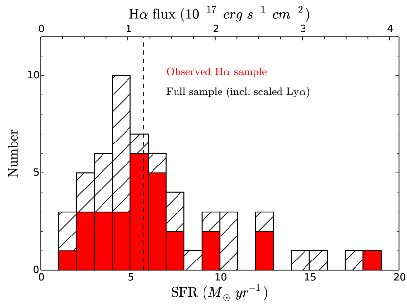
Figure 1.— The distribution of star-formation rates for the 60 LAEs presented in this paper. Red histogram gives the distribution of measured H$\alpha$ fluxes and dust-corrected H$\alpha$ star-formation rates (SFR). The hatched histogram includes estimates for LAEs with no current $K$-band measurements; for these objects, the H$\alpha$ flux is estimated from the measured Ly$\alpha$ flux and the median Ly$\alpha$/H$\alpha$ ratio among the objects with measured H$\alpha$ fluxes. The H$\alpha$ flux and SFR from the full LAE composite spectrum (Fig. 4) is shown by the dashed line.

Star-formation rates (SFRs) are calculated for the 28 LAEs with H$\alpha$ measurements using the Kennicutt (1998) relation, as displayed in Fig. 1. We apply a uniform dust-correction based on the average nebular reddening estimated in Sec. 4.4 ($E(B-V)=0.06$; Eq. 7) and a Cardelli et al. (1989) extinction curve, which produces a 15% increase in the estimated star-formation rates. For the LAEs without current H$\alpha$ flux measurements, we estimate SFRs based on the narrowband Ly$\alpha$ flux, scaled by the median Ly$\alpha$/H$\alpha$ flux ratio from the objects with direct H$\alpha$ measurements ($\langle f_{\textrm{\scriptsize{Ly$\alpha$}}}/f_{\textrm{\scriptsize{H$\alpha$}}}\rangle=3.1$). The distribution of H$\alpha$- and Ly$\alpha$-derived SFRs are statistically indistiguishable, as shown in Fig. 1. The median LAE H$\alpha$ SFR = 5.3 $\rm M_{\odot}$ yr^-1, which is consistent with the value estimated from the composite $K$-band spectrum (5.7$\pm$1.4 $\rm M_{\odot}$ yr^-1) and significantly lower than the H$\alpha$-derived SFRs typical of the KBSS LBG sample we consider here (median SFR $=27$ $\rm M_{\odot}$ yr^-1; Strom et al. 2016).

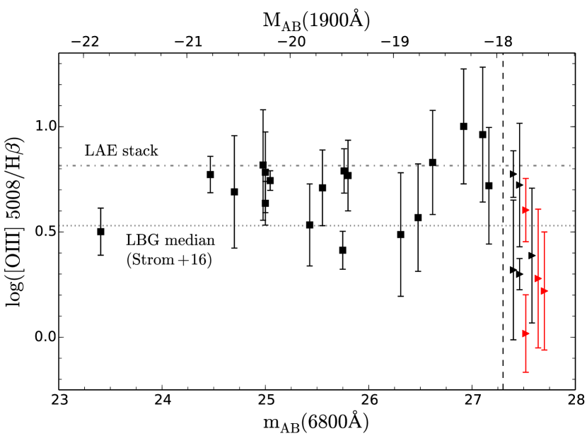
Figure 2.— The ratio O3 $\equiv$ log([O III] $\lambda$5008/H$\beta$) vs. $\mathcal{R}$-band magnitude for 27 LAEs with $>$3$\sigma$ detections of both H$\beta$ and [O III] $\lambda$5008. Black squares denote LAEs with measured $\mathcal{R}$ magnitudes, while triangles denote LAEs fainter than the 3$\sigma$ limit $\mathcal{R}>27.3$ (vertical dashed line), which are given arbitrary horizontal offsets for clarity. Red points are also undetected in deep HST/WFC F160W images sampling the rest-frame optical wavelengths (3$\sigma$ depth $m_{\textrm{\scriptsize{AB,F160W}}}>28.1$). The dot-dashed horizontal line is the best-fit value of O3 from our composite LAE spectrum (Fig. 3, Table 3), while the dotted horizontal line corresponds to the median value for all KBSS LBGs with $>$3$\sigma$ detections of both H$\beta$ and [O III] $\lambda$5008. The LAEs generally have elevated values of O3 with respect to the LBGs, with the exception of the faintest LAEs. These faint objects are consistent with the turnover in O3 that occurs at extremely low oxygen abundances (12 + log(O/H) $\ll$ 8.3, $Z_{\textrm{\scriptsize{neb}}}\ll 0.4Z_{\odot}$) as discussed in Sec. 6.3.

Fig. 2 displays the O3 ratio for each of the 27 LAEs with $>$3$\sigma$ detections of both H$\beta$ and at least one of [O III] $\lambda$5008 or [O III] $\lambda$4960. Although the uncertainties are large on many of the individual measurements, the ratios are generally elevated with respect to the typical LBG value of O3 $\approx 0.5$. An exception to this trend occurs for the LAEs with the faintest continuum luminosities ($M_{\textrm{\scriptsize{AB}}}(1900$Å$)\gtrsim-18$; $L\lesssim 0.06L_{*}$ from Reddy et al. 2008), which have lower O3 ratios than the average LAEs or even the typical LBG values. These faintest LAEs are undetected in our $\mathcal{R}$ band images, and four of them have no detection in deep, 8000 second images from HST/WFC3 in the F160W filter, setting a (point source) limiting magnitude $m_{\textrm{\scriptsize{AB}}}(1.6\mu$m$)>28.1$ (3$\sigma$). The low O3 ratios of these sources suggest that the faintest LAEs have either lower excitation states than typical galaxies at these redshifts or very low metallicities ($Z_{\textrm{\scriptsize{neb}}}<0.1Z_{\odot}$). These objects are discussed in more detail in Sec. 6.3.

3.2. Measurements from composite spectra

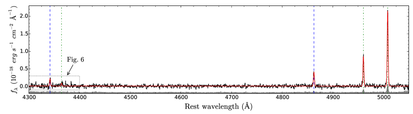
Figure 3.— Full composite $H$ band spectrum of 60 LAEs (218 object-hours). Red line is the fit to the composite spectrum as described in Sec. 3.2.2, and grey shaded region shows the 1$\sigma$ bootstrap errors on the composite spectrum, offset for clarity. Blue dashed lines correspond to the rest-wavelengths of H$\gamma$ and H$\beta$, while green dot-dashed lines denote the wavelengths of $[$O III$]$ $\lambda$4364 and [O III] $\lambda\lambda$4960,5008 (Table 3). Dotted-line box in the lower left contains the region of the spectrum that Fig. 6 displays in greater detail.

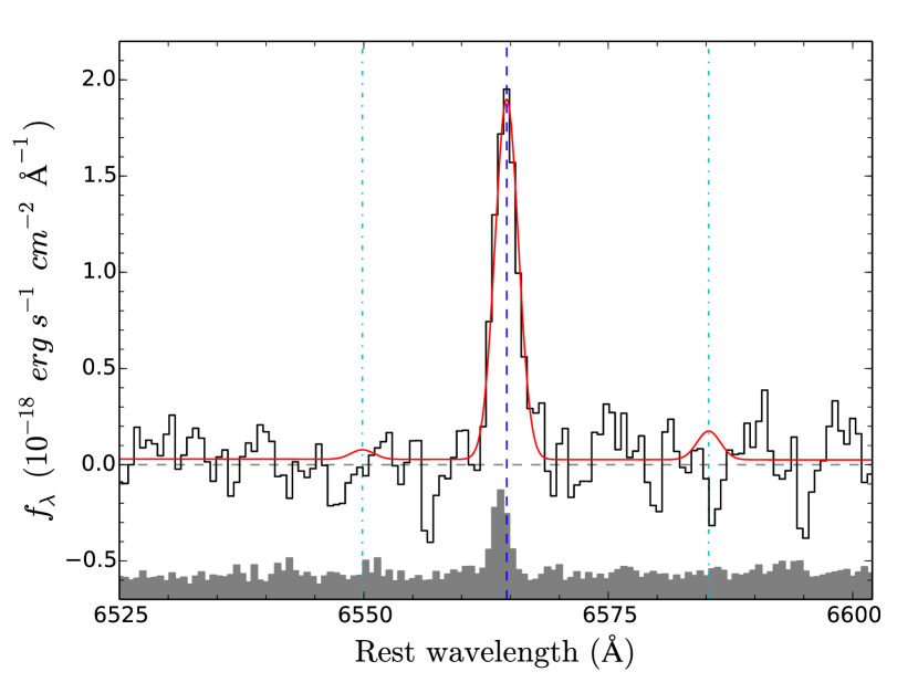
Figure 4.— Composite $K$ band spectrum of 28 LAEs (83 object-hours), as in Fig. 3. Red line is the fit to the composite spectrum including the 2$\sigma$ upper limit on the total [N II] $\lambda\lambda$6549,6585 emission (cyan dot-dashed lines; Table 3). Blue dashed line indicates the rest wavelength of H$\alpha$.

3.2.1 Creation of composite spectra

In addition to our measurements of emission lines from individual LAEs, we construct composite LAE spectra to obtain high-S/N measurements typical of the population of LAEs and various sub-populations.

The $H$-band composite spectra are constructed as follows. Before the individual spectra are combined, they are resampled to the same rest-frame wavelength scale of 0.45 Å pix^-1 (equivalent to MOSFIRE’s native $H$-band pixel scale of 1.63 Å pix^-1 in the observed frame shifted to $z\approx 2.56$) spanning the wavelengths 4200Å $<\lambda_{\textrm{\scriptsize{rest}}}<$ 5050Å. An exposure mask is created to isolate the spectral region that falls on the detector within the MOSFIRE $H$ passband. In order to account for OH sky-line contamination, we resample the error vector output by the MOSFIRE reduction pipeline to the same wavelength scale as the science spectrum. The $H$-band error vector is extremely flat across the band between the sky lines, so we identify sky lines as those regions of the error spectrum that exceed twice the median error value. The exposure mask is then set to zero for these regions, such that contaminated pixels receive zero weight in the final stack. Typically, 19$\pm$1% of pixels in each spectrum are removed by this algorithm. In addition, some of our objects have particularly high background noise at $\lambda_{\textrm{\scriptsize{rest}}}\lesssim 4400$Å; this is especially evident for the Q1603 spectra, which have shorter exposure times and lie at lower redshifts (such that these rest wavelengths fall nearer to the blue edge of the MOSFIRE $H$ band). We therefore set the exposure mask to zero in any regions of a given spectrum that lie at $\lambda_{\textrm{\scriptsize{rest}}}<4400$Å and have local noise properties $>$2$\times$ the median noise level of the other $H$-band spectra at the same rest-frame wavelengths.

Because the rest-optical continuum is not detected in any individual LAE spectrum, we do not scale the spectra by continuum magnitude before stacking. The final $H$ composite spectrum for a given set of LAEs is then the mean of all their $H$-band spectra, scaled by their mask-correction factors and weighted by their corresponding exposure masks (which reflect both the relative differences in exposure time per object and the removal of contaminated or unobserved regions of each spectrum). Our $H$-band spectra have very little difference in exposure times, so each LAE receives approximately equal weight in the final $H$-band composite. The composite spectrum of all 55 LAEs with $H$-band spectroscopy is given in Fig. 3.

Our $K$-band composite spectrum is constructed in a similar manner: the individual object spectra are resampled to a constant pixel scale of 0.6 Å pix^-1 for 5400Å $<\lambda_{\textrm{\scriptsize{rest}}}<$ 6800Å (the native MOSFIRE $K$ pixel scale is 2.17 Å pix^-1 in the observed frame). The $K$-band error spectrum has less sky-line contamination than the $H$ band, but it also has a strong wavelength dependence at $\lambda_{\textrm{\scriptsize{obs}}}\gtrsim 2.1\mu$m, where the uncertainty is dominated by thermal noise. In order to remove sky-line-contaminated regions of the spectra before combining, we construct a smoothed noise spectrum for each object using a 25-pixel boxcar kernel and median averaging within the kernel. This process produces a good approximation to the thermal noise profile with minimal contributions from sky lines. Pixels where the error spectrum is greater than 2.5$\times$ this local smoothed noise spectrum are then identified as sky-line-contaminated regions and do not contribute to the composite spectrum. Only 5$\pm$1% of pixels are removed from each $K$-band spectrum via this process. The composite spectrum of all 28 LAEs with $K$-band spectroscopy is given in Fig. 4.

We estimate uncertainties in the $H$ and $K$ composite spectra by means of a bootstrap procedure. For each sample of $N_{\textrm{\scriptsize{obj}}}$ LAE spectra used to construct a composite spectrum, a bootstrap spectrum is generated by constructing a bootstrap sample of size $N=N_{\textrm{\scriptsize{obj}}}$ (where spectra are drawn randomly with replacement) averaging them into a bootstrap composite spectrum using the same weighting and masking procedures described above. This process is repeated 300 times to construct an array of bootstrap composite spectra, and the uncertainty at each pixel is estimated from the standard deviation of bootstrap composite values at that pixel. In this way, the bootstrap uncertainties represent the combination of measurement uncertainties and the true variation of LAE spectra within each sample. These uncertainties are shown in Figs. 3 & 4 as a grey shaded region below each spectrum.

In Sec. 5, we discuss composite spectra for high-$W_{\rm Ly\alpha}$ and low-$W_{\rm Ly\alpha}$ subgroups of our LAE sample. These composites are constructed in a manner identical to the above, including the creation of their boostrap uncertainty vectors. The groups are split at the median photometric Ly$\alpha$ equivalent width of our sample; LAEs with $W_{\rm Ly\alpha}>57$Å contribute to the high-$W_{\rm Ly\alpha}$ composite spectrum (30 $H$-band spectra, 12 $K$-band), while the LAEs with $W_{\rm Ly\alpha}<57$Å contribute to the low-$W_{\rm Ly\alpha}$ composite spectrum (25 $H$-band, 16 $K$-band).

3.2.2 Fitting composite spectra

Table 3Emission Line Measurements

Transition	$\lambda_{\textrm{\scriptsize{rest}}}$ (Å)	Flux ($10^{-18}$ cgs)
H$\gamma$	4341.67	1.63$\pm$0.54
$[$O III$]$ $\lambda$4364	4364.44	0.62$\pm$0.22
H$\beta$	4862.72	3.44$\pm$0.58
$[$O III$]$ $\lambda$4960	4960.30	7.47$\pm$1.09
$[$O III$]$ $\lambda$5008	5008.24	18.92$\pm$2.72
$[$O III$]$ $\lambda$5008 (corr)	5008.24	22.41$\pm$3.28
$[$N II$]$ $\lambda$6549	6549.86	$<$ 0.31
H$\alpha$	6564.61	11.76$\pm$2.92
$[$N II$]$ $\lambda$6585	6585.27	$<$0.93

The composite spectra were fit using a set of gaussian line profiles and a linearly-varying continuum. For the $H$-band composite, five emission lines are fit simultaneously: H$\gamma$, [O III] $\lambda$4364, H$\beta$, [O III] $\lambda$4960, and [O III] $\lambda$5008. The gaussian line profiles are constrained to be centered on the vacuum wavelength $\lambda_{\textrm{\scriptsize{rest}}}$ of the associated transition (see Table 3), and all lines are constrained to have the same velocity width, but the amplitude of each emission line is fit independently. With a linear continuum component, there are a total of 8 free parameters in the fit. The results of the fit are displayed in Fig. 3, and the fit line fluxes are given in Table 3.

The $K$-band composite is fit in a similar manner, but with only 3 fit emission lines: [N II] $\lambda$6549, H$\alpha$, and [N II] $\lambda$6585, for a total of 6 free parameters in the fit. The results of this fit are also given in Fig. 4 and Table 3.

Line flux uncertainties are estimated from the samples of bootstrap spectra. For each bootstrap spectrum, the emission lines and continuum level are fit as described above, where each free parameter in the full composite fit is allowed to vary for each bootstrap spectrum as well. For each bootstrap spectrum, the line fluxes and best-fit velocity width are measured. The 1$\sigma$ uncertainty in the measurement of these parameters in the composite spectrum is then estimated from the distribution of values from the 300 bootstrap spectra; specifically, from the central interval including 68% of corresponding parameter values among the bootstrap spectra (Table 3). Note that the actual uncertainty in our measurement of a given emission line in the composite spectrum is often significantly smaller than this value, but we present these uncertainties to reflect the range of values associated with a “typical” sample of similarly-selected LAEs.

In the same way, the uncertainty in the line ratios within a band (e.g., N2, O3; Table 4) are estimated by computing the corresponding line ratio for each bootstrap spectrum and measuring the size of the interval encompassing 68% of the bootstrap line ratio measurements. Line fluxes and ratios are calculated in the same manner for the low-$W_{\rm Ly\alpha}$ and high-$W_{\rm Ly\alpha}$ composite spectra. Note that this this strategy must differ for cross-band line ratios (e.g., H$\alpha$/H$\beta$), where a different number of individual spectra contribute to the bootstrap composite for each emission line (see Sec. 4.4 below).

In Sec. 4 below, we discuss the constraints inferred from the emission line ratio measurements and limits in these composite LAE spectra.

4. Measurements from optical line ratios

4.1. N2-BPT constraints

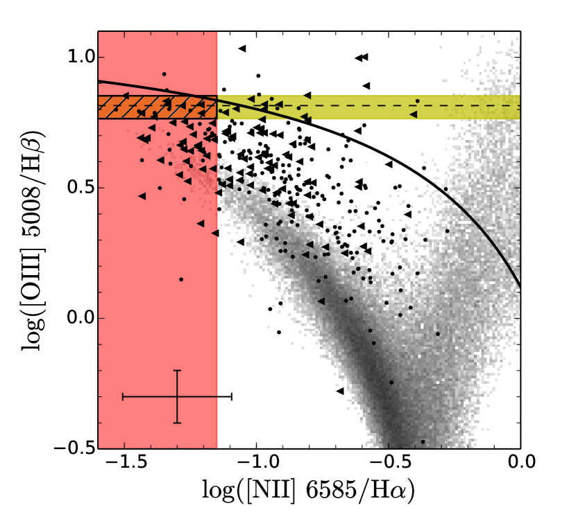
Figure 5.— N2-BPT diagram (Baldwin et al., 1981) with SDSS $z\sim 0$ galaxies (gray, log density scaling) and KBSS LBGs (Strom et al. 2016; black points and 2$\sigma$ limits; cross in lower left shows typical errors). Yellow bar is the O3 measurement for the LAE $H$-band composite spectrum (Fig. 3), and pink region is current 2$\sigma$ limit on N2 from the $K$-band composite (Fig. 4). Black hatches denote the combined constraints from both measurements, which show that the LAEs are consistent with the extreme high-ionization, low-metallicity tail of the LBG population. For comparison, the black line shows the “maximum starburst” curve from Kewley et al. (2001).

The Baldwin et al. (1981) “BPT” diagrams provide a simple means of classifying the sources of ionizing radiation and physical gas properties in galaxies. In particular, the N2-BPT diagram compares the ratio log([O III] $\lambda$5008/H$\beta$) (hereafter, O3) to log([N II] $\lambda$6585/H$\alpha$) (hereafter, N2), which separate into two clear tracks for low-redshift galaxies. These emission lines also have the advantage of lying close to one another in wavelength, such that neither ratio is strongly affected by dust attenuation or cross-band calibration errors. Fig. 5 displays the N2-BPT diagram for local galaxies from the Sloan Digital Sky Survey (SDSS DR7; Abazajian et al. 2009) along with high-redshift measurements described below.

In the N2-BPT diagram, star-forming galaxies occupy the locus of objects at low N2, while AGN-dominated and composite objects form a “fan” that extends toward high O3 and N2. The star-forming locus is extremely tight, with 90% of star-forming galaxies falling within $\pm 0.1$ dex of the ridgeline (Kewley et al., 2013). The small degree of scatter in this sequence suggests that the intensity and shape of the stellar ionizing fields and the properties of the ionized gas are tightly coupled by one or more physical properties that vary along the locus. In particular, these galaxies are known to follow a sequence in metallicity (Dopita et al., 2000), with low-metallicity galaxies or H II regions exhibiting high O3 and low N2 (the upper left of the N2-BPT), while those with high metallicities occupy the lower right of the diagram.

As described in Sec. 1, however, recent surveys at higher redshifts indicate that typical galaxies at $z\approx 2-3$ occupy a locus that is approximately as tight as that measured in the local Universe (Steidel et al., 2014), but offset toward higher O3 and/or N2 (Steidel et al., 2014; Masters et al., 2014; Shapley et al., 2015; Sanders et al., 2015; Masters et al., 2016; Strom et al., 2016). Strom et al. (2016) use detailed studies of the nebular spectra of KBSS LBGs to determine that this offset primarily corresponds to high nebular excitation (i.e., a vertical shift in the N2-BPT plane) at a given stellar mass and gas-phase metallicity. The black points in Fig. 5 represent LBGs from the KBSS, as described by Strom et al. (2016). Triangles represent 2$\sigma$ upper limits on N2, and the cross in the lower left shows the median uncertainty of the points with detections. While measurement uncertainties contribute significantly to the observed scatter, the KBSS LBGs appear to roughly span the region between the SDSS locus and the black solid line, which denotes the “maximum starburst” limit from Kewley et al. (2001).

The measurements from the LAE composite spectra are displayed as colored bands in the plot. The horizontal dashed line is the best-fit O3 measurement from the composite $H$-band spectrum in Fig. 3, and the yellow region encompasses the 68% confidence interval on this value (accounting for the scatter among the combined spectra through the bootstrap procedure described in Sec. 3.2.1). The red band corresponds to the 2$\sigma$ upper limit and confidence interval on N2 from the composite $K$-band spectrum in Fig. 4. The average N2-BPT line ratios of our LAEs are thus localized to the far upper left corner of the plot, where the two regions overlap (the values of the line ratios and their uncertainties are given in Table 4).

Given the correspondence between the N2-BPT locus and nebular metallicity, typical LAEs appear to be similar to the lowest-metallicity LBGs in the KBSS sample. In fact, Erb et al. (2016) isolate the most extreme 5% of LBGs in the upper left of the N2-BPT plane (effectively constructing a metallicity-selected sample of galaxies) and find that they occupy almost exactly the same region as that defined by our composite LAE constraints: O3 $\geq 0.75$ and N2 $\leq-1.1$. These “extreme” LBGs are found to have similar physical and spectroscopic properties to the low-redshift population of rare, compact, high-excitation galaxies known as “Green Peas” (Cardamone et al., 2009; Amorín et al., 2012; Jaskot & Oey, 2013), including high Ly$\alpha$ equivalent widths, Ly$\alpha$ escape fractions, and ionization states (O32; Table 2 & Sec. 5.2.2). In T15, we also showed that these Green Peas (as presented by Henry et al. 2015) show similar Ly$\alpha$ and kinematic properties to the KBSS-Ly$\alpha$ LAEs. Given that a simple selection based on Ly$\alpha$ emission and continuum faintness apparently isolates the most extreme subset of objects with respect to $z\approx 0$ galaxies and $z\approx 2-3$ LBGs, it is worthwhile to consider the mechanisms by which the Ly$\alpha$ emission and nebular properties of these galaxies are related; we discuss this topic in depth in Sec. 5.

4.2. [O III] auroral line and gas temperature

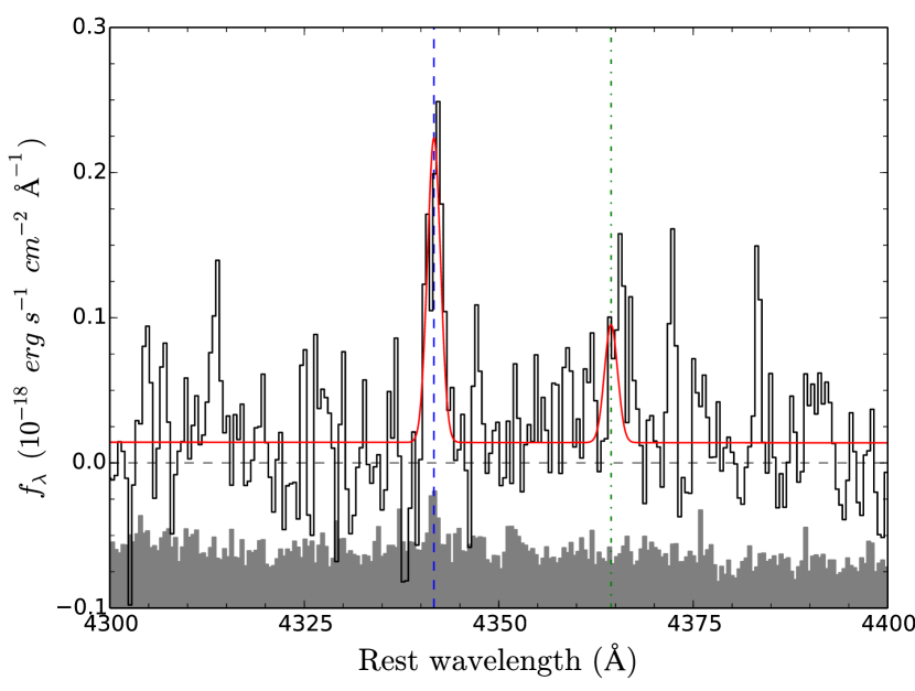
Figure 6.— Zoomed-in version of the composite $H$-band spectrum from Fig. 3 at the location of the H$\gamma$ (blue dashed line) and [O III] $\lambda$4364 (green dashed line) emission lines. Fit (red) and bootstrap uncertainty vector (grey) are as described in the above figures.

The [O III] $\lambda$4364 transition is another emission line of particular interest for studies of star-forming galaxies. Because this auroral emission line corresponds to the transition from the second excited state to the first excited state, its measurement in combination with the nebular transition (from the first excited state to the ground state) provides a direct measure of the electronic level populations and thus the temperature of the O III gas. As this temperature is set in part by metal-line-dominated cooling in the ionized nebular regions, the auroral and nebular line measurements can also be converted into an estimate of the gas-phase metallicity, often described as the “direct method” metallicity measurement.

The region of the $H$-band composite spectrum near the [O III] $\lambda$4364 auroral line is reproduced in more detail in Fig. 6. As described above, each of the five lines in the $H$-band spectrum are fit simultaneously (along with the continuum) and constrained to have the same velocity width and redshift. These constraints significantly improve our ability to determine the [O III] $\lambda$4364 flux. In particular, the nearby H$\gamma$ emission line provides a valuable cross-check of the wavelength and flux calibrations at these wavelengths, which lie near the blue edge of the MOSFIRE $H$ band. Notably, the H$\gamma$ line is detected with high significance, the emission is centered at the proper rest-wavelength, and the measured flux is consistent with the expected H$\gamma$/H$\beta$ ratio under case-B recombination and $E(B-V)\approx 0$, as discussed in Sec. 4.4 below. For these reasons, we expect that the derived [O III] $\lambda$4364 flux is well-determined, despite the relatively marginal (2.8$\sigma$) detection of the peak.

The [O III] line fluxes are given in Table 3. As described above, we use the $\lambda$4960 line to correct the [O III] $\lambda$5008 line flux because of the uncertain flux calibration at the extreme red end of the MOSFIRE $H$ band. The ratio of auroral to nebular O III line flux $R_{\textrm{\scriptsize{O3}}}\equiv$ [O III] ($\lambda$4364)/($\lambda\lambda$4960,5008) is therefore equivalent to [O III] ($\lambda$4364)/(4$\times\lambda$4960) in our measurement, and we find $R_{\textrm{\scriptsize{O3}}}=2.0\pm 0.7$%. We use the iterative procedure described by Izotov et al. (2006) (reproduced from Aller 1984) to determine the O III electron temperature $T_{3}$, finding a converged value $T_{3}=1.78\pm 0.33\times 10^{4}$K, where the uncertainty reflects the 1$\sigma$ range of $R_{\textrm{\scriptsize{O3}}}$ ratios measured in our bootstrap spectra.

4.3. Gas-phase metallicity estimates

Given a measurement of the electron temperature, ionic abundances (and the “direct method” oxygen abundance) can be estimated via the ratios of additional metal-ion and hydrogen emission lines, as further discussed by Izotov et al. (2006). Using the formulae fit in that paper, we calculate the ionic O III abundance 12 + log(O⁺⁺/H⁺) = $7.68\pm 0.16$. The estimation of the elemental O/H abundance requires an ionization correction that can only be measured with the addition of emission line measurements from other oxygen ions, which are not currently measured for the LAE sample presented here. However, there is a close relationship between O32 and O3 among the KBSS LBG galaxies (see further discussion in Sec. 5.2.2), such that the LBGs with O3 $\approx 0.8$ have O32 $\approx 0.7-1.0$ (that is, nebular [O III] emission 5$-$10$\times$ stronger than that of [O II]; Strom et al. 2016). For this reason, the contribution of O II to the total oxygen abundance is likely to be small among the highly-excited LAEs, and we calculate an ionization correction based on a likely value of O32 $=0.7$. The temperature of the O II zone of the H II region is typically lower than that of the O III zone, and the difference in temperature (the “$T_{2}-T_{3}$” relation) is typically found to be $T_{2}\approx 0.7\times T_{3}-3000$K by photoionization models (e.g., Campbell et al. 1986; Garnett 1992; Izotov et al. 2006; Pilyugin et al. 2009), consistent with recent direct observations of $T_{2}$ in H II regions of local star-forming galaxies (Brown et al., 2014; Berg et al., 2015).

Under these assumptions, the inferred ionic O II abundance is 12 + log(O⁺/H⁺) = $7.17\pm 0.19$, where the uncertainty includes only the range of $T_{3}$ consistent with our bootstrap spectra. If the true O32 ratio for our LAE spectra is greater than the assumed value of 0.7, or if the O II temperature is higher than that predicted by our assumed $T_{2}-T_{3}$ relation, then the contribution of O II to the total oxygen abundance is even smaller. Conversely, Andrews & Martini (2013) suggest that the formula above overestimates $T_{2}$ by $\Delta T_{2}\approx 1300$K; applying such a shift would increase our estimate of 12 + log(O⁺/H⁺) to 7.28.

Assuming that O III and O II are the dominant states of oxygen in the nebular regions (and likewise that the neutral fraction of hydrogen is negligible in these regions), the inferred “direct” oxygen abundance is thus the sum of the above ionic abundances, and we estimate a total oxygen abundance 12 + log(O/H)${}_{\textrm{\scriptsize{dir}}}$ = 7.80$\pm$0.17 ($Z_{\textrm{\scriptsize{neb}}}\approx 0.13Z_{\odot}$). As above, the uncertainty corresponds to the statistical uncertainty from our bootstrap measurements; for comparison, assuming O32 = 1.0 or using the Andrews & Martini (2013) $T_{2}$ calibration would shift our inferred oxygen abundance by $-$0.06 dex or +0.03 dex, respectively.

However, a larger source of systematic uncertainty may come from the tendency of collisionally-excited lines (CELs) including the O III lines discussed above to overestimate the volume-averaged electron temperature of a cloud. This effect may occur due to the temperature sensitivity of the emissivity of CELs, which causes any luminosity-weighted $T_{e}$ measurement to be biased toward the highest-temperature regions of the nebula. Such a bias may cause metallicity estimates from CELs to underestimate the metallicity relative to that inferred from recombination lines (RELs) and stellar spectra. This effect is seen in the detailed spectroscopic LBG study described by Steidel et al. (2016), who find an offset between the nebular O/H abundance inferred from the [O III] “direct” method and that obtained through comprehensive modeling of the nebular and stellar spectra. Steidel et al. find an offset consistent with that measured from CELs and RELs in local low-metallicity dwarf galaxies by Esteban et al. (2014):

$$\rm{log(O/H)_{\textrm{\scriptsize{REL}}}}-\rm{log(O/H)_{\textrm{\scriptsize{CEL}}}}=0.24\pm 0.02\,\,\rm{dex}$$ (1)

In constrast, Bresolin et al. (2016) find a low-metallicity REL-CEL offset of similar magnitude, but they suggest that CELs are more accurate than RELs by comparing both estimators to stellar metallicities collected from the literature. Given that the results of Steidel et al. (2016) appear to corraborate the Esteban et al. (2014) offset at $z\approx 2-3$, we apply a +0.24 dex correction to our “direct” abundance measurement described above in order to determine our final estimate of the nebular gas-phase metallicity:

$$12+\rm{log(O/H)} = 8.04\pm 0.19$$ (2)

$$Z_{\textrm{\scriptsize{neb}}} = 0.22^{+0.12}_{-0.08}Z_{\odot}$$ (3)

where the uncertainty reflects both the statistical uncertainties from our bootstrap analysis and the statistical uncertainty in the Esteban et al. (2014) calibration, but it does not include the systematic uncertainty in the application of the REL-CEL offset, nor those associated with the O II abundance discussed above.

As described in Sec. 4.1, the O3 and N2 ratios are also often used as gas-phase metallicity indicators (the “strong-line” metallicity indicators N2 and O3N2, Table 2) through local calibrations to $T_{e}$-based measurements. As discussed by Steidel et al. (2014, 2016), these strong-line indicators are based on the adherence of star-forming galaxies to their locus in the local N2-BPT plane, and thus require recalibration at high redshift, where this locus is offset toward higher values of nebular excitation. Lacking a direct calibration of these relationships at $z\approx 2$, we use the recent calibration of O3N2 by Strom et al. (2016), which is based on a local set of extragalactic H II regions from Pilyugin et al. (2012). Using this relation, our best-fit measurement of O3, and our 2$\sigma$ upper limit on N2, we obtain the following limit:

$$12+\rm{log(O/H)_{\textrm{\scriptsize{O3N2,Strom16}}}}<8.17$$ (4)

which is consistent with the corrected direct estimate in Eq. 2. For comparison, the widely-used N2 and O3N2 abundance calibrations by Pettini & Pagel (2004) also produce estimates consistent with our direct-method determination:

$$12+\rm{log(O/H)_{\textrm{\scriptsize{O3N2,PP04}}}}<8.10$$ (5)

$$12+\rm{log(O/H)_{\textrm{\scriptsize{N2,PP04}}}}<8.24\,\,.$$ (6)

4.4. Balmer decrement and extinction measurements

The above inferences are based on line ratios (O3, N2, R${}_{\textrm{\scriptsize{O3}}}$) that fall within a single MOSFIRE band. However, not all the LAEs in our sample have both $H$ and $K$ band detections, which means that cross-band line ratios (such as the Balmer decrement, H$\alpha$/H$\beta$) cannot be measured for the full sample of spectra. Eleven LAEs in our sample have $>$3$\sigma$ detections of both H$\alpha$ and H$\beta$. Among these spectra, the average ratio is H$\alpha$/H$\beta$ = 2.92$\pm$0.45. The uncertainty is the 1$\sigma$ error on the average estimated via a modified bootstrap technique similar to that described in Sec. 3.2.1 above, but modified so that the same randomized set LAEs contribute to each bootstrap sample of both H$\alpha$ (in the $K$ band) and H$\beta$ (in the $H$ band).

We estimate the average extinction from the Balmer decrement assuming a Cardelli et al. (1989) Milky-Way extinction curve and the tabulated intrinsic H$\alpha$/H$\beta$ ratios from Brocklehurst (1971). Typically, extinction measurements for high-redshift galaxies assume an electron temperature $T_{e}\approx 10^{4}$ K, corresponding to an intrinsic ratio H$\alpha$/H$\beta$ = 2.89. However, our measurement of the [O III] $\lambda$4364 line implies a somewhat higher value of $T_{e}\approx 1.8\times 10^{4}$ K, so we adopt the Balmer decrement value for $T_{e}=2\times 10^{4}$ K from Brocklehurst (1971): H$\alpha$/H$\beta$ = 2.74. Choosing the higher intrinsic ratio would decrease our inferred extinction by a small amount, as discussed below.

Under these assumptions, our Balmer decrement measurements correspond to a reddening, $V$-band extinction, and H$\alpha$ extinction as follows:

$$\textrm{E}(B-V) = 0.06\pm 0.12$$ (7)

$$A_{V} = 0.20\pm 0.39$$

$$A_{\textrm{\scriptsize{H$\alpha$}}} = 0.16\pm 0.32\,\,.$$

Choosing an intrinsic ratio H$\alpha$/H$\beta$ = 2.89 would imply $E(B-V)=0.01\pm 0.12$, consistent with the above measurement. For comparison, we also calculate the extinction inferred from the total $H$ and $K$ stacks using the uncorrected H$\alpha$ and H$\beta$ values from Table 3 (despite corresponding to different samples of LAEs). From these values, we calculate a Balmer decrement H$\alpha$/H$\beta$ = 3.37, or E$(B-V)$ $=0.2$ under the assumptions above. This value is slightly higher than that inferred from the matched samples of detected H$\alpha$ and H$\beta$ lines, likely reflecting the fact that our current $K$-band spectra are shallower on average than those in the $H$ band, such that bright H$\alpha$ lines are over-represented in the full $K$ stack. We therefore take the extinction inferred from the matched sample (Eq. 7) to best represent our full LAE population, and the dust-corrections used to derive LAE star-formation rates in Fig. 1 are based on this value.

5. The nebular origins of Ly$\alpha$ emission

In order to determine the physical properties of LAEs, it is important to understand the physical drivers of their most salient characteristic: strong Ly$\alpha$ emission. Toward this end, we here consider the relationship between the nebular properties described above and the Ly$\alpha$ emission of our LAE sample, as well as that of a comparison sample of LBGs from the KBSS (Steidel et al., 2014, 2016; Strom et al., 2016). The KBSS and KBSS-Ly$\alpha$ represent the richest current sample of combined Ly$\alpha$ and rest-optical spectroscopy for star-forming galaxies at any redshift, so these surveys are a powerful tool for dissecting the physical differences between galaxies selected by Ly$\alpha$ emission and those selected by continuum brightness, while also establishing the variation in net Ly$\alpha$ emissivity with galaxy properties across the combined population of LAEs and LBGs.

5.1. The BPT-Ly$\alpha$ relation

Table 4LAE and LBG Subsamples

Sample	Subsample	$N_{\textrm{\scriptsize{obj}}}$	$\langle W_{\textrm{\scriptsize{Ly$\alpha$}}}\rangle$	SFR	N2	O3	H$\alpha$/H$\beta$	E($B-V$)
	all	60	56.2Å	7.7$\pm$1.9	0$<$ $-$1.15	0.82$\pm$0.05	2.92$\pm$0.45	0.06$\pm$0.12
LAEs	$W_{\textrm{\scriptsize{Ly$\alpha$,phot}}}>57$Å	30	79.0Å	4.5$\pm$1.0	$<$ $-$0.94	0.90$\pm$0.09	2.63$\pm$1.03	$<$ $-$0.29
	20Å$<W_{\textrm{\scriptsize{Ly$\alpha$,phot}}}\leq 57$Å	30	24.7Å	14.4$\pm$4.40	$<$ $-$1.07	0.76$\pm$0.07	3.19$\pm$0.38	0.15$\pm$0.11
	$W_{\textrm{\scriptsize{Ly$\alpha$,spec}}}>20$Å	48	47.3Å	19.3$\pm$2.2	$-$1.12$\pm$0.12	0.73$\pm$0.02	3.77$\pm$0.19	0.27$\pm$0.05
LBGs	$0$ $\leq W_{\textrm{\scriptsize{Ly$\alpha$,spec}}}\leq 20$Å	1040	07.8Å	21.0$\pm$1.4	$-$1.00$\pm$0.06	0.64$\pm$0.02	3.95$\pm$0.12	0.32$\pm$0.03
	$W_{\textrm{\scriptsize{Ly$\alpha$,spec}}}<0$	2160	0$-$7.6Å+	21.1$\pm$0.8	$-$0.90$\pm$0.03	0.54$\pm$0.02	4.08$\pm$0.09	0.35$\pm$0.02

Figure 7.— N2-BPT diagram as in Fig. 5, but with KBSS LBGs color-coded by Ly$\alpha$ equivalent width ($W_{\textrm{\scriptsize{Ly$\alpha$}}}$). Blue points show Ly$\alpha$ in emission, while red points show Ly$\alpha$ in absorption. The sizes of the points correspond to the absolute value of $W_{\textrm{\scriptsize{Ly$\alpha$}}}$. Error bars in lower left correspond to the median 1$\sigma$ uncertainties on the detected KBSS points. Blue diamonds in the upper right corner correspond to KBSS objects with spectroscopically-identified AGN emission (Steidel et al., 2014). The black hatched region shows the confidence interval for the LAE stacks. Solid black line denotes the “maximum starburst” curve from Kewley et al. (2001), while the dashed black line shows the Strom et al. (2016) KBSS locus. There is a general trend for high-$W_{\textrm{\scriptsize{Ly$\alpha$}}}$ galaxies to occupy the upper left of the diagram (near the LAE sample), whereas low-$W_{\textrm{\scriptsize{Ly$\alpha$}}}$ objects occupy the lower right. The physical origins of this trend are analyzed throughout Sec. 5.

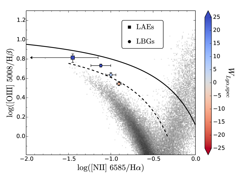
Figure 8.— N2-BPT diagram as in Figs. 5 & 7, but with KBSS points stacked in three subsamples according to their value of $W_{\textrm{\scriptsize{Ly$\alpha$}}}$ (Table 4). Error bars correspond to the 1$\sigma$ uncertainties from bootstrap resampling. In analogy to the other points, the LAE stacks are presented with a point at the best fit value of O3 and the 1$\sigma$ limit on N2, with error bars indicating the 1$\sigma$ uncertainty on O3 and the 2$\sigma$ upper limit on N2. The solid black line denotes the “maximum starburst” curve from Kewley et al. (2001), while the dashed black line shows the Strom et al. (2016) KBSS locus. A strong trend is visible as $W_{\rm Ly\alpha}$ increases toward the low-metallicity end of the N2-BPT locus.

As discussed above in Sec. 4.1, the N2-BPT diagram provides a useful discriminant of the physical properties of ionized regions within a galaxy, which constrains the metallicity of both the gas itself and the sources of ionizing radiation, including properties of the stellar populations.

Fig. 7 displays the N2-BPT line ratios of 336 KBSS galaxies with $>$5$\sigma$ ($>$3$\sigma$, $>$3$\sigma$) detections of H$\alpha$ (H$\beta$, [O III] $\lambda$5008) and spectroscopic measurements of their Ly$\alpha$ equivalent widths, $W_{\textrm{\scriptsize{Ly$\alpha$,spec}}}$. While there is considerable scatter in the nebular line ratios at a given value of $W_{\textrm{\scriptsize{Ly$\alpha$,spec}}}$, there is also a clear trend such that Ly$\alpha$-emitting LBGs ($W_{\textrm{\scriptsize{Ly$\alpha$,spec}}}>0$, blue points) have high values of O3 and low values of N2 (i.e., they lie in the upper-left region of the N2-BPT space), whereas Ly$\alpha$ absorbers ($W_{\textrm{\scriptsize{Ly$\alpha$,spec}}}<0$, red points) preferentially occupy the opposite corner of parameter space. Objects with spectra indicating AGN activity (e.g., broad nebular emission lines and/or strong C IV or He II UV emission) are denoted by diamonds in the plot; these objects show high ratios of both O3 and N2 similar to the spectra of low-redshift AGN.

The region of the N2-BPT parameter space consistent with our composite LAE spectra (as in Fig. 5) is displayed as the hatched region in Fig. 7. The nebular line properties of the composite LAE spectra are generally consistent with those of the KBSS LBGs with the highest values of $W_{\textrm{\scriptsize{Ly$\alpha$}}}$.

Fig. 8 compares the composite LAE line ratios to analogous stacked measurements of subsamples of the KBSS LBGs, which are described in Table 4. The KBSS subsamples are divided on the basis of $W_{\textrm{\scriptsize{Ly$\alpha$}}}$: Ly$\alpha$-absorbers ($W_{\textrm{\scriptsize{Ly$\alpha$,spec}}}<0$), weak Ly$\alpha$-emitters ($0<W_{\textrm{\scriptsize{Ly$\alpha$,spec}}}<20$Å), and strong Ly$\alpha$-emitters ($W_{\textrm{\scriptsize{Ly$\alpha$,spec}}}>20$Å). For each subsample, all spectra are combined for which the MOSFIRE $H$ and $K$ spectra cover the rest-wavelengths of all 4 of the N2-BPT diagnostic lines: H$\beta$, [O III] $\lambda$5008, H$\alpha$, and [N II] $\lambda$6585. Objects spectroscopically identified as AGN (marked as diamonds in Fig.  7) are excluded from the stacks, leaving a total of 368 LBGs. In order to ensure that each object receives the same weighting in both the $H$ and $K$ composites while maximizing their S/N, both spectra for each object are weighted by the inverse-variance at the wavelength of the [N II] $\lambda$6585 line (generally the weakest of the N2-BPT diagnostic lines in this sample). The line ratios measured for each composite spectrum are listed in Table 4 and displayed in Fig. 8. For comparison, the LAE composite measurements are plotted in Fig. 8 as a point at the best-fit value of O3 and the 1$\sigma$ upper limit of N2, with error bars reflecting the 68% confidence interval on O3 and the 2$\sigma$ upper limit of N2. The value of $W_{\textrm{\scriptsize{Ly$\alpha$,spec}}}$ is measured for each LAE and LBG sample directly from the corresponding composite UV spectrum by comparing the measured Ly$\alpha$ line flux (without correcting for Ly$\alpha$ slit losses) to the UV continuum flux on the red side of the Ly$\alpha$ line, as is described for measurements of individual LBG spectra in Sec. 2.3.

As in Fig. 7, Fig. 8 shows a clear trend between the value of $W_{\textrm{\scriptsize{Ly$\alpha$}}}$ for a given subsample and its position in the N2-BPT plane. The composite measurements parallel the locus of SDSS N2-BPT measurements, albeit with an offset consistent with previous studies of high-redshift star-forming galaxies, as discussed above. Notably, our current limits on the typical properties of faint LAEs appear consistent with the trend seen in the LBG composites; the “BPT offset” of the full LAE composite measurement may be slightly greater than that of the KBSS composites, but the LAE measurement may actually be more consistent with the SDSS locus depending on the (currently unmeasured) typical LAE N2 ratio. Rather than investigating the source of this offset, we therefore consider what physical galaxy properties are changing along the locus of $z\approx 2-3$ LAEs and LBGs that accompany or drive the variation in Ly$\alpha$ emissivity.

The highest-$W_{\textrm{\scriptsize{Ly$\alpha$}}}$ objects and composite spectra in our sample are those that lie nearest to the low-metallicity end of the SDSS galaxy locus (see discussion in Sec. 4.1). Given the correlation between gas-phase metallicity and dust content, this may suggest that our observed trend is a signature of the previously-studied tendency of LAEs to exhibit lower dust attenuation with respect to continuum-selected galaxies. In such a scenario, the variation in net Ly$\alpha$ emissivity along the N2-BPT locus (as parameterized by $W_{\textrm{\scriptsize{Ly$\alpha$}}}$) is primarily a variation in the physics of Ly$\alpha$ escape, which is expected to depend sensitively on the distribution of gas and dust within the interstellar medium of the host galaxies.

However, Steidel et al. (2014) demonstrate that gas-phase metallicity has more minor effects on the position of individual galaxies within the locus of star-forming galaxies at $z\approx 2-3$ compared to $z\approx 0$. Rather, the primary determinants of the N2-BPT line ratios in LBGs galaxies appear to be the relative hardness of the incident radiation field and the effective ionization parameter $n_{\gamma}/n_{H}$, the dimensionless ratio of hydrogen-ionizing photons to hydrogen atoms within the ionized star-forming regions. This ionization parameter may also be expressed as the factor $U\equiv\Phi_{H}/n_{H}c$, where $n_{H}$ is the number density of hydrogen atoms (including ionized, neutral, and molecular) in the star-forming regions and $\Phi_{H}$ is the surface flux of H-ionizing photons incident on the illuminated face of the H II region, as defined by Osterbrock & Ferland (2006). A recent, thorough discussion of the ionization parameter, its various definitions, and its observational constraints in the star-forming regions of $z\approx 2-3$ galaxies is given by Sanders et al. (2016). We refer to the ionization parameter as $U$ in the sections that follow in order to compare our measurements to predictions from the Cloudy photoionization code (Ferland et al., 2013), which explicitly defines $U$ as described above, but we note that the physical interpretation of this ratio can become ambiguous when divorced from the specific plane-parallel or spherical ionization geometries assumed by photoionization models (as discussed by Steidel et al. 2014).

Crucially, the dependence of a galaxy’s nebular line ratios on $U$ and the radiation field hardness means that these ratios are strongly determined by the overall normalization and shape of the stellar radiation field at photon energies 1 Ryd $<E_{\gamma}\lesssim$ 4 Ryd, which in turn means that the N2-BPT line ratios may be at least as sensitive to properties of the young stellar populations within the H II regions as to the intrinsic properties of the ionized gas. Specifically, Steidel et al. (2014) argue that the nebular line spectra of $z\approx 2-3$ LBGs are best-explained by populations of hot massive stars, and Steidel et al. (2016) interpret combined deep rest-UV and nebular line spectra of these LBGs in light of binary evolution models in low-metallicity stellar populations, which naturally produce hotter, harder ionizing spectra than typical stellar models over long ($\gg$Myr) timescales as described in Sec. 1.

In the section below, we consider two possible modes by which the nebular spectra of these galaxies may be tied to Ly$\alpha$ emissivity: variation in the extinction of Ly$\alpha$ photons by interstellar dust (which may also appear as reddening in the nebular spectra), or variation in the Ly$\alpha$ production rate via recombination in ionized star-forming regions (which may produce changes in the observed nebular excitation).

5.2. Origin of the BPT-Ly$\alpha$ relation

5.2.1 Ly$\alpha$ emission vs. dust attenuation

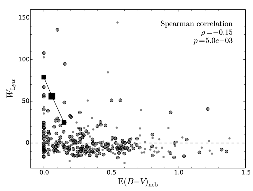
Figure 9.— The spectroscopic equivalent width of Ly$\alpha$ ($W_{\rm Ly\alpha}$) vs. the nebular reddening E$(B-V)$ inferred from the Balmer decrement measurement for individual KBSS LBGs (grey points) and KBSS-Ly$\alpha$ LAE composite spectra (large black square indicates the full sample, while smaller squares denote the low-$W_{\rm Ly\alpha}$ and high-$W_{\rm Ly\alpha}$ subsamples). Circled points are those with S/N $>5$ in H$\alpha$/H$\beta$, the limit proposed by Strom et al. (2016) for secure measurements of E$(B-V)$. The horizontal dashed line demarcates the boundary between Ly$\alpha$-absorbers ($W_{\rm Ly\alpha}<0$) and Ly$\alpha$-emitting LBGs ($W_{\rm Ly\alpha}>0$). The results of a non-parametric Spearman correlation test on the LBG values are displayed in the upper right, which indicates that $W_{\rm Ly\alpha}$ has only modest dependence on the inferred reddening and attenuation by dust. The LAEs have much higher values of $W_{\rm Ly\alpha}$ than reddening-matched LBGs.

We investigate the modulation of Ly$\alpha$ emissivity by dust by comparing the relationship between $W_{\rm Ly\alpha}$ and the nebular reddening E$(B-V)$ estimated from the Balmer decrement (as described in Sec. 4.4) for each of the KBSS LBG spectra and the LAE composites (including the low-$W_{\textrm{\scriptsize{Ly$\alpha$}}}$, high-$W_{\textrm{\scriptsize{Ly$\alpha$}}}$, and combined subsamples). The inferred nebular reddening and Ly$\alpha$ equivalent width for each LBG (from the set of 336 objects with full N2-BPT and Ly$\alpha$ line coverage) and LAE composite is shown in Fig. 9. An association of high-$W_{\rm Ly\alpha}$ LBGs with low values of E$(B-V)$ is visible, although there are several LBGs with high values of both $W_{\rm Ly\alpha}$ and E$(B-V)$. A non-parametric Spearman rank-correlation test finds a weak negative correlation ($\rho=-0.15$) between $W_{\rm Ly\alpha}$ and E$(B-V)$ for the LBG sample with moderate significance ($p=5\times 10^{-3}$). Strom et al. (2016) find that some KBSS LBGs exhibit unphysical dust-corrected line ratios (e.g., in the R23-O32 plane) when corrections are applied based on low-S/N measurements of E$(B-V)$${}_{\textrm{\scriptsize{neb}}}$, suggesting a limit of H$\alpha$/H$\beta$ $>5$$\sigma$ for reliable estimates of the dust attenuation. The 200 LBGs in the sample that meet this cut (including the uncertainty in the cross-band calibration) are circled in Fig. 9; they occupy a very similar distribution to the lower-S/N observations, with a comparable correlation ($\rho=-0.21$) and significance ($p=3\times 10^{-3}$). The LAE composite spectra (black squares) appear to show a much stronger relationship with E$(B-V)$, but we have insufficient data to quantify this trend among the LAEs alone. Notably, however, the LAE $W_{\rm Ly\alpha}$ measurements are clearly inconsistent with the distribution of LBG points at similar values of E$(B-V)$: at fixed reddening, the LAE composites have significantly higher values of $W_{\rm Ly\alpha}$ than the LBG points. It appears, therefore, that a difference in dust attenuation is insufficient to explain either the variation of $W_{\rm Ly\alpha}$ among the KBSS LBG sample or the differences between the LAE and LBG populations.

Although it is expected that absorption by dust is the primary mechanism for the destruction of Ly$\alpha$ photons in galaxies, there have been previous observational indications that dust and Ly$\alpha$ emission can co-exist. While no previous sample of $z\approx 2-3$ galaxies has had sufficient measurements of both rest-UV and rest-optical emission line spectra to quantify the relationship between $W_{\rm Ly\alpha}$ and nebular E$(B-V)$ in detail, studies of the broadband spectral energy distributions of LAEs have found galaxies exhibiting both strong Ly$\alpha$ emission and large inferred stellar E$(B-V)$ (Kornei et al., 2010; Hagen et al., 2014; Matthee et al., 2016), including objects with $E(B-V)_{\textrm{\scriptsize{stars}}}\gtrsim 0.4$. The 14 “extreme” LBGs in the Erb et al. (2016) sample have higher $W_{\rm Ly\alpha}$ and lower E$(B-V)$${}_{\textrm{\scriptsize{neb}}}$ than average KBSS LBGs, but include individual objects with inferred reddening as high as $E(B-V)_{\textrm{\scriptsize{neb}}}\approx 0.34$ in the sample of objects with H$\alpha$/H$\beta$ S/N $>10$ (or as high as $E(B-V)_{\textrm{\scriptsize{neb}}}\approx 0.95$ with no S/N cut). In the full sample of KBSS LBGs presented here, there are galaxies with $W_{\rm Ly\alpha}>20$Å which exhibit reddening as high as $E(B-V)_{\textrm{\scriptsize{neb}}}=1.2$, even with the Strom et al. (2016) cut on S/N. Conversely, there is a substantial population of LBGs with low values of E$(B-V)$ and low or no net Ly$\alpha$ emission: the average LBG with E$(B-V)$${}_{\textrm{\scriptsize{neb}}}$ consistent with our full LAE composite ($E(B-V)_{\textrm{\scriptsize{neb}}}\lesssim 0.06$, approximately the lowest quartile in the LBG E$(B-V)$${}_{\textrm{\scriptsize{neb}}}$ distribution) is actually a net absorber of Ly$\alpha$ photons in slit spectroscopy (median $W_{\textrm{\scriptsize{Ly$\alpha$,spec}}}=-2.0$Å).

While neither E$(B-V)$${}_{\textrm{\scriptsize{stars}}}$ nor E$(B-V)$${}_{\textrm{\scriptsize{neb}}}$ is a perfect proxy for the attenuation of Ly$\alpha$ photons by dust, E$(B-V)$${}_{\textrm{\scriptsize{neb}}}$ has the advantage of tracing the attenuation of photons from the same star-forming regions where Ly$\alpha$ photons are expected to originate (rather than the diffuse interstellar dust distribution traversed by photons from spatially-extended populations of stars). We suggest, therefore, that our observations are the strongest evidence yet that low dust content, while associated with Ly$\alpha$ escape, is neither necessary nor sufficient for producing strong Ly$\alpha$ emission in galaxy spectra. The trend in $W_{\rm Ly\alpha}$ with position on the N2-BPT diagram is therefore unlikely to be a product of the association of gas-phase metallicity with dust-to-gas ratio.

5.2.2 Ly$\alpha$ emission vs. nebular excitation

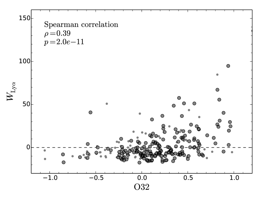
Figure 10.— The spectroscopic equivalent width of Ly$\alpha$ ($W_{\rm Ly\alpha}$) vs. the dust-corrected O32 ratio for individual KBSS LBGs (grey points). Circled points are those with more secure dust corrections, as in Fig. 9. Despite substantial scatter, there is a stronger trend than is seen for $W_{\rm Ly\alpha}$ vs. E$(B-V)$.

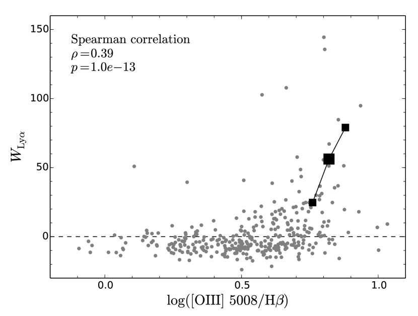
Figure 11.— The spectroscopic equivalent width of Ly$\alpha$ ($W_{\textrm{\scriptsize{Ly$\alpha$}}}$) vs. the [O III]/H$\beta$ ratio–a measure of nebular excitation–for individual KBSS LBGs (grey points) and LAE composites (large black square indicates the full sample, while smaller squares denote the low-$W_{\rm Ly\alpha}$ and high-$W_{\rm Ly\alpha}$ subsamples), as in Fig. 9. A strong trend is present, with the LAE stacks displaying similar excitation-matched $W_{\rm Ly\alpha}$ values to the LBGs, indicating that the observed $W_{\rm Ly\alpha}$ is strongly modulated by the physics governing Ly$\alpha$ production within H II regions.

We now consider the second mode by which the nebular spectra of galaxies may be linked to their Ly$\alpha$ emission: the ionization and recombination processes within their star-forming regions. There are multiple reasons why the ionization and excitation states of gas in H II regions may be associated with Ly$\alpha$ emission. Stronger sources of ionizing photons (e.g., hotter populations of massive stars) will both increase the typical ionization state of their surrounding gas and result in a larger production rate of Ly$\alpha$ photons (as well as other products of recombination emission). Secondly, density-bounded H II regions (those in which the star-forming cloud becomes completely ionized) will be more transparent to escaping Ly$\alpha$ photons than those that are surrounded by thick shells of neutral gas. Similarly, such density-bounded H II regions may exhibit high average ionization ratios (e.g., O32; Table  2), as discussed in Sec.  7

We have not obtained measurements of the [O II] $\lambda\lambda$3727,3729 emission-line doublet (which lies in the MOSFIRE $J$ band at $z\approx 2.1-2.6$) for our LAE sample, but we can investigate the trend between O32 and $W_{\rm Ly\alpha}$ in our comparison sample of KBSS spectra. Fig. 10 shows the O32 ratio for the subset of the N2-BPT LBG sample that also have a $>$3$\sigma$ detection of [O II] $\lambda\lambda$3727,3729 (275 objects; 82% of the objects included in the full N2-BPT sample). The O32 ratios have been dust-corrected assuming the E$(B-V)$${}_{\textrm{\scriptsize{neb}}}$ measurements described above and a Cardelli et al. (1989) extinction curve. As in Fig. 9, circled points are those meeting a 5$\sigma$ cut on the H$\alpha$/H$\beta$ dust correction and MOSFIRE $J$-$H$ cross-calibration.

Substantial scatter is present among the values of $W_{\rm Ly\alpha}$ at fixed O32, although a Spearman rank-correlation test shows a much stronger trend ($\rho=0.39$; $p=2\times 10^{-11}$) than is seen in the $W_{\rm Ly\alpha}$-E$(B-V)$ relationship. The objects with the most secure dust corrections and cross-band flux calibrations (175 objects) show a still stronger correlation ($\rho=0.45$; $p=3\times 10^{-10}$). The median $W_{\rm Ly\alpha}$ measurement among LBGs in the upper quartile of O32 (O32 $>0.46$) is $W_{\rm Ly\alpha}=8.5$Å, indicating that these objects are net Ly$\alpha$ emitters (unlike the lowest quartile of LBGs in E$(B-V)$). Among the KBSS-LBG sample, it therefore appears that O32 is a better predictor of strong Ly$\alpha$ emission than E$(B-V)$.

While we cannot directly measure O32 for the LAE samples presented here, the O3 ratio is a related measure of the nebular excitation properties of galaxies. Although O3 is sensitive to the gas-phase oxygen abundance at very low metallicities ($Z\lesssim 0.2Z_{\odot}$, Sec. 6), it is much more sensitive to the ionization parameter and hardness of the incident spectrum at more intermediate sub-solar metallicities typical of the KBSS LBGs ($0.3Z_{\odot}\lesssim Z\lesssim 0.9Z_{\odot}$; Steidel et al. 2014, 2016; Strom et al. 2016). Furthermore, the O32 and O3 ratios are closely correlated; the Spearman rank correlation between both values is $\rho=0.74$ for the 175 KBSS LBGs with the highest-confidence dust-corrected O32 values. The O3 ratio also has the advantage of requiring no dust correction or cross-band calibration, as both lines lie near each other in the MOSFIRE $H$ band at $z\approx 2-2.6$.

The O3 ratio is therefore a useful discriminant for comparing the excitation properties of the LBG and LAE samples and their variation with $W_{\rm Ly\alpha}$, as is shown in Fig. 11. A Spearman test among the 336 LBGs in the N2-BPT sample yields $\rho=0.39$ and $p=10^{-13}$ for the O3-$W_{\rm Ly\alpha}$ correlation, approximately as strong as the O32-$W_{\rm Ly\alpha}$ correlation. Furthermore, the KBSS galaxies with O3 $>0.82$, consistent with the full LAE composite measurement, are typically strong Ly$\alpha$ emitters (median $W_{\rm Ly\alpha}=14.6$Å). In general, the LAEs have quite similar values of $W_{\rm Ly\alpha}$ to excitation-matched samples of KBSS LBGs, in contrast to the distribution of attenuation-matched LBGs in Fig. 9. Similarly, there are very few Ly$\alpha$-emitting KBSS LBGs with low O3 values, including only two objects with O3 $<0.5$ and $W_{\rm Ly\alpha}>14$Å.

The substantial scatter in $W_{\rm Ly\alpha}$ at fixed excitation is not surprising, given the multiplicity of factors that govern Ly$\alpha$ escape. Nevertheless, it appears that the net Ly$\alpha$ emission that escapes star-forming galaxies at small galactic radii (that is, the Ly$\alpha$ emission to which slit spectroscopy is most sensitive) remains closely coupled to the properties of their ionized birthplaces despite the subsequent interactions of these photons with the surrounding interstellar and circumgalactic media.

6. Photoionization Model Comparison

6.1. Model parameters

The nebular spectra of star-forming galaxies are sensitive to a broad range of physical parameters, including the electron density $n_{e}$, ionization parameter $U$, gas-phase metallicity and elemental abundance patterns; the stellar metallicity and abundance patterns, ages, initial-mass function (IMF), and evolutionary properties of the embedded stars; as well as the foreground extinction. Many of these properties can produce degenerate effects on galaxy spectra, particularly when only a few nebular lines are observed. Given that our current measurements are limited to the brightest lines in the $H$ and $K$ atmospheric windows, we use the trends established among the brighter LBG samples in Sec. 5.2 and the more detailed modeling presented by Steidel et al. (2016, hereafter S16) and Strom et al. (2016) to constrain the range of physically-motivated model parameters.

With this in mind, we run a grid of Cloudy (Ferland et al., 2013) photoionization models over a range of physical gas parameters and sources of incident radiation consistent with these previous studies. We vary the ionization parameter $U$ over the range $-3\leq$ log$U$ $\leq-1.5$, where log$U$ is varied in steps of $\Delta$log$U$ = $0.1$. The gas-phase metallicity is varied over the range $0.1\leq Z_{\textrm{\scriptsize{neb}}}/Z_{\odot}\leq 1.0$ in steps of $\Delta$$Z=0.1$, as well as $0.01\leq Z_{\textrm{\scriptsize{neb}}}/Z_{\odot}\leq 0.1$ in steps of $\Delta$$Z=0.01$. The Cloudy models assume a solar abundance pattern from Asplund et al. (2009), but we scale the output nitrogen-based line ratios according to the relation between N/O and O/H suggested by Strom et al. (2016):

$$\textrm{log(N/O)}=-13.48+1.45\times[12+\textrm{log(O/H)}]\,.$$ (8)

However, this relationship is not intended to be applied at the lowest metallicities, where many surveys of local low-metallicity galaxies and H II regions have found that the N/O vs. O/H relation becomes flat, with log(N/O) $\approx-1.5$ at low O/H. We therefore impose a minimum value of log(N/O) $=-1.5$, which applies at all inferred oxygen abundances less than 12 + log(O/H) = 8.26 ($Z_{\textrm{\scriptsize{neb}}}=0.4Z$).

We fix the electron density $n_{e}=300$ cm^-3 as in S16, consistent with the measured electron densities from the KBSS and MOSDEF surveys ($n_{e}\approx 200-360$ cm^-3; Steidel et al. 2014, 2016; Sanders et al. 2016; Strom et al. 2016). While individual galaxy spectra in these surveys exhibit a wide range of $n_{e}$, Strom et al. (2016) demonstrate that there is no trend between inferred $n_{e}$ and offset from the low-redshift N2-BPT locus, and we likewise find no correlation between inferred $n_{e}$ and stellar mass or Ly$\alpha$ equivalent width.

We perform our photoionization modeling using incident stellar radiation fields from the latest version of two spectral-synthesis codes: Starburst99 (Leitherer et al., 2014) and BPASSv2 (Eldridge & Stanway, 2016; Stanway et al., 2016), the latter of which includes explicit modelling of the effects of binary interactions on stellar evolution. Several models from each model suite are described in detail in S16. In that paper, deep rest-UV and rest-optical spectra are modeled simultaneously to constrain the properties of the stellar populations in KBSS LBGs, finding that the composite spectra require $Z_{*}\ll 0.008$ and are best fit by $Z_{*}=0.001-0.002$ ($Z_{*}/Z_{\odot}=0.07-0.14$). As in S16, we explicitly decouple the metallicity of our stellar models ($Z_{*}$) from the gas-phase metallicity input to the photoionization code ($Z_{\textrm{\scriptsize{neb}}}$); the physical rationale for this choice is dicussed below.

We adopt the best-fit $Z_{*}=0.07Z_{\odot}$ BPASSv2 model from S16 as our fiducial stellar population, which is denoted as BPASSv2-z001-300bin in that paper. The model assumes a Salpeter (1955) IMF (power law index of $-2.35$) and a stellar mass range of $0.5\leq M_{*}\leq 300$. For comparison, we also consider the Starburst99 model denoted as S99-v00-z001 in S16, which has the default Kroupa (2001) IMF (power law index of $-2.30$) and a stellar mass range of $0.5\leq M_{*}\leq 100$. We also consider models with $Z_{*}=0.002$ ($Z_{*}=0.14Z_{\odot}$) that are otherwise identical to the $Z_{*}=0.001$ models. All our stellar models assume a continuous star-formation history of 100 Myr. As noted in S16, these models do not change appreciably in the far-UV after a few $\times$10⁷ years, which is approximately the central dynamical time of the KBSS-Ly$\alpha$ LAEs and thus the shortest likely timescale for galaxy-scale bursts of star formation in these systems.

As shown in S16, small differences in the IMF power-law index do not significantly affect the output nebular line ratios: increasing (flattening) the slope of the Starburst99 IMF from $-2.3$ to $-2.0$ or even $-1.7$ does not reproduce the high O3 and R23 ratios observed in the LBG composite spectrum by S16. Changing the upper-mass cutoff of the IMF (i.e., from 100 $\rm M_{\odot}$ to 300 $\rm M_{\odot}$) does harden the EUV spectrum, although to a lesser extent than the inclusion of massive stellar binaries. Even the Starburst99 models from Leitherer et al. (2014) that include rapid stellar rotation do not produce the significant changes to the EUV spectral shape that are required to explain the nebular line ratios of the KBSS LBGs. In addition, models which exclude binary interactions (e.g., both the Starburst99 models and the BPASS non-binary models) do not generate He II $\lambda$1640 emission (which is seen in the S16 rest-UV LBG composite) in continuous star-formation over long ($>$10Myr) timescales. In fact, S16 find that the BPASSv2-z001-300bin model is the only spectrum considered that produces the full suite of observed rest-UV and rest-optical line measurements for the LBG stack. Nonetheless, in order to investigate the dependence of the inferred nebular LAE properties on the assumed stellar population, we consider both the Starburst99 and BPASSv2 models in our analysis.

6.2. Modeling the composite spectra

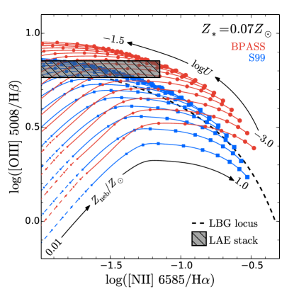
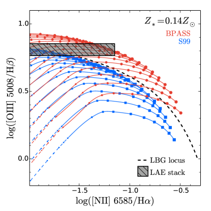
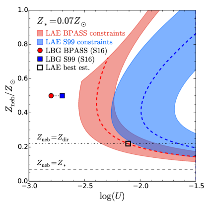
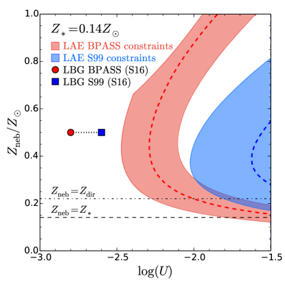
Figure 12.— (Top) N2-BPT predictions for the Cloudy photoionization models given an input spectrum from BPASS (red) or S99 (blue) stellar populations. The left panel uses a $Z_{*}=0.07Z_{\odot}$ ($Z_{*}=0.001$) input model, while the right panel has $Z_{*}=0.14Z_{\odot}$ ($Z_{*}=0.002$). Grey hatched region denotes the measurement of O3 and 2$\sigma$ limit on N2 from the full LAE composite spectra (Figs. 3 & 4). Photoionization models are plotted as a function of $Z_{\textrm{\scriptsize{neb}}}$ for each value of $U$, with $-3\leq$ log$U$ $\leq-1.5$ (with $U$ increasing from the bottom to the top of the panel) and $0.01\leq Z_{\textrm{\scriptsize{neb}}}/Z_{\odot}\leq 1.0$. Marker size increases with increasing metallicity, and $Z_{\textrm{\scriptsize{neb}}}<0.1$ is shown with a dashed line. (Bottom) Constraints on the gas-phase metallicity $Z_{\textrm{\scriptsize{neb}}}$ and ionization parameter $U$ from the LAE composite spectra and the Cloudy models presented in the top panels. Red regions correspond to the parameters consistent with the LAE N2-BPT limits assuming a BPASS stellar population (with stellar metallicity as above), while the blue regions correspond to parameter constraints assuming a S99 stellar population. Dashed curves correspond to parameters that reproduce the best-fit measurement of O3 from the LAE composite spectrum. The horizontal dot-dash line corresponds to the gas-phase metallicity estimated via the auroral [O III] transition (Sec. 4.2), and the black box represents our best estimate of the LAE nebular and stellar parameters: ($Z_{*}$, $Z_{\textrm{\scriptsize{neb}}}$, log$U$) = (0.07, 0.022, -2.1). The dashed line represents the gas-phase metallicity equal to the input stellar metallicity in each panel: it is evident that the two metallicities are difficult to reconcile assuming solar abundance patterns. Red circles (blue squares) represent the best-fit values of $Z_{\textrm{\scriptsize{neb}}}$ inferred for the LBG composite spectra by Steidel et al. (2016) using the same stellar BPASS (S99) model spectra, although the S99 models fail to reproduce other nebular ratios discussed in that paper. The LAE spectra require significantly enhanced ionization parameters with respect to the LBG samples.

The Cloudy predictions for both the S99-v00-z*** models (hereafter “the S99 models”) and the BPASSv2-z***-300bin models (hereafter “the BPASS models”) in the N2-BPT plane are given in the top panels of Fig. 12 for a range of gas-phase metallicities and ionization parameters. Values of $Z_{\textrm{\scriptsize{neb}}}$ between grid points are interpolated using a cubic spline. For both stellar metallicities considered, the BPASS model produces higher average excitation (O3) values at fixed $Z_{\textrm{\scriptsize{neb}}}$ and $U$. Note that O3 increases with $Z_{\textrm{\scriptsize{neb}}}$ at low $Z_{\textrm{\scriptsize{neb}}}$ for all models up to a maximum at $Z_{\textrm{\scriptsize{neb}}}\approx 0.4$ and then decreases as $Z_{\textrm{\scriptsize{neb}}}$ is increased further. N2, however, increases monotonically with increasing $Z_{\textrm{\scriptsize{neb}}}$.

The constraints on the typical LAE excitation are plotted as the shaded box in each panel (as above, we use the 68% confidence interval in O3 and the 2$\sigma$ upper limit on N2). For the S99 models, only the highest ionization parameters are able to reproduce the best-fit LAE line ratios (particularly for $Z_{*}=0.14Z_{\odot}$ models), while the BPASS stellar models are relatively insensitive to $Z_{*}$ and are able to reproduce the LAE measurements over a range of values of $Z_{*}$, $Z_{\textrm{\scriptsize{neb}}}$, and $U$.

The bottom panels of Fig. 12 show these constraints explicitly. In each panel, the red shaded region corresponds to the values of ($U$, $Z_{\textrm{\scriptsize{neb}}}$) that produce N2 and O3 ratios consistent with the LAE composite measurements using the BPASS stellar models. Similarly, the blue region corresponds to the range of allowed parameters assuming the S99 input stellar spectra. The blue and red dashed curves correspond to the values ($U$, $Z_{\textrm{\scriptsize{neb}}}$) that produce the best-fit value of O3 = $0.82$ (Table 4) and are consistent with the upper limit on N2. As in the top panels, values are interpolated in between grid points using a cubic spline. Formally, values of $Z_{\textrm{\scriptsize{neb}}}\gtrsim Z_{\odot}$ are allowed for both of the $Z_{*}=0.07Z_{\odot}$ stellar models, although the BPASS model cannot reproduce the best-fit observed O3 ratio and N2 limit with $Z_{\textrm{\scriptsize{neb}}}>0.7$. Stronger constraints on the N2 ratio are needed to cross-check the typical gas-phase metallicity ($Z_{\textrm{\scriptsize{neb}}}\approx 0.2Z_{\odot}$) inferred from the [O III] $\lambda$4364 measurement in Sec. 4.2. However, we note that $Z_{\textrm{\scriptsize{neb}}}$ less than $\sim$0.2 would require extremely high values of the ionization parameter (log$U\gtrsim-2.0$).

Given that the galaxies in the LBG sample have luminosities and masses $\sim$10$\times$ larger than the typical LAEs, we find it likely that the LAEs have average stellar metallicities at least as low as the metallicity favored for the LBGs in S16 ($Z_{*}=0.07Z_{\odot}$). Under this assumption, our LAE observations strongly favor values of $Z_{\textrm{\scriptsize{neb}}}$ significantly higher than the modeled stellar metallicities, similar to the effect seen in the S16 and Strom et al. (2016) LBG samples. As described in those works, this apparent discrepancy is likely a manifestation of the same non-solar abundance ratios in both the stars and gas. The shape of the model stellar spectrum is most strongly dependent on those elements that dominate the opacity of the stellar photosphere (i.e., iron), which are produced by Type Ia SNe at late times. Conversely, the nebular metallicity constraints are most sensitive to the species which dominate the cooling of the $\sim$$10^{4}$ K gas, dominated by oxygen that is released in the comparatively prompt Type II SNe. S16 and Strom et al. (2016) therefore argue that the apparent $Z_{\textrm{\scriptsize{neb}}}/Z_{*}$ ratio should be interpreted as a non-solar O/Fe abundance ratio, and these discrepancies signify the $\alpha$-enhancement of young galaxies and star-forming regions at high redshift. Our LAE measurements are consistent with this interpretation.

The ionization parameter of the gas has even stronger constraints from our LAE compsite spectra. Using the BPASS models, the best-fit O3 ratio can only be reproduced with log$U>-2.4$ (log$U>-2.3$) for $Z_{*}=0.07Z_{\odot}$ ($Z_{*}=0.14Z_{\odot}$). The dependence of the minimum value of $U$ on stellar metallicity reflects the fact that the same nebular excitation can be achieved with a lower value of $U$ (that is, fewer photons per hydrogen atom) for a harder incident spectrum. This effect is seen more strongly for the S99 models, which have significantly softer EUV spectra: the $Z_{*}=0.07Z_{\odot}$ S99 model requires log$U>-2.0$ to reproduce the best-fit O3 value regardless of $Z_{\textrm{\scriptsize{neb}}}$, and the $Z_{*}=0.14Z_{\odot}$ S99 model requires log$U>-1.65$. If $Z_{\textrm{\scriptsize{neb}}}=0.22Z_{\odot}$ is assumed, log$U\gg-1.7$ is required.

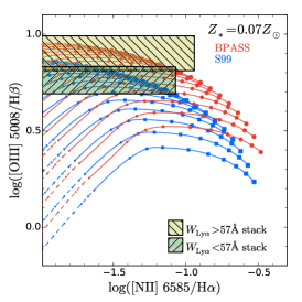
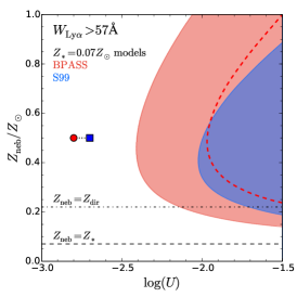
Figure 13.— (Left) N2-BPT predictions for the Cloudy photoionization models as in the top row of Fig. 12. Green (yellow) shaded region denotes the constraints from the low-$W_{\rm Ly\alpha}$ (high-$W_{\rm Ly\alpha}$) composite LAE spectra. The input spectra have $Z_{*}/Z_{\odot}=0.07$ as in the left panels of Fig. 12 (Center) Constraints on $Z_{\textrm{\scriptsize{neb}}}$ and $U$ for the high-$W_{\rm Ly\alpha}$ sample corresponding to the green region in the left panel. Annotation matches the bottom panels of Fig. 12. (Right) Constraints on $Z_{\textrm{\scriptsize{neb}}}$ and $U$ for the low-$W_{\rm Ly\alpha}$ sample (yellow region in the left panel).

S16 infer tight constraints on both $U$ and $Z_{\textrm{\scriptsize{neb}}}$ from their LBG composite spectra, and these values are also plotted on the bottom panels of Fig. 12. The best-fit values ($U$, $Z_{\textrm{\scriptsize{neb}}}$) are shown as calculated using the same BPASS and S99 model spectra used for the LAE constraints in each plot. As described above, the S99 models provide a poor match for full set of line ratios in the S16 spectrum, but we note that the required ionization parameter for the LAE composite measured here is significantly higher than the best-fit value for the S16 LBG composite even if we remain agnostic as to the choice of stellar population model.

In Fig. 13, we display similar constraints for the high-$W_{\rm Ly\alpha}$ and low-$W_{\rm Ly\alpha}$ LAE samples. Only the $Z_{*}=0.07Z_{\odot}$ models are displayed, since the BPASS predictions change only slightly with $Z_{*}$ and the S99 models with $Z_{*}=0.14Z_{\odot}$ struggle to reproduce the measurements from the full composite spectrum. The models in the left panel of Fig. 13 are the same as those presented in the first panel of Fig. 12, but the hatched regions correspond to the constraints on N2 and O3 from the high-$W_{\rm Ly\alpha}$ and low-$W_{\rm Ly\alpha}$ LAE composite spectra (Table 4). The low-$W_{\rm Ly\alpha}$ LAE subsample (green region in the left panel of Fig. 13) has lower average excitation, such that it can be reproduced by both BPASS and S99 stellar models with intermediate values of $U$. The constraints on $Z_{\textrm{\scriptsize{neb}}}$ and $U$ for this sample are displayed in the center panel of Fig. 13. The allowed range of ionization parameters shifts closer to the LBG values from S16 (the red circle and blue square in the same panel) compared to the values estimated from the full LAE stack.

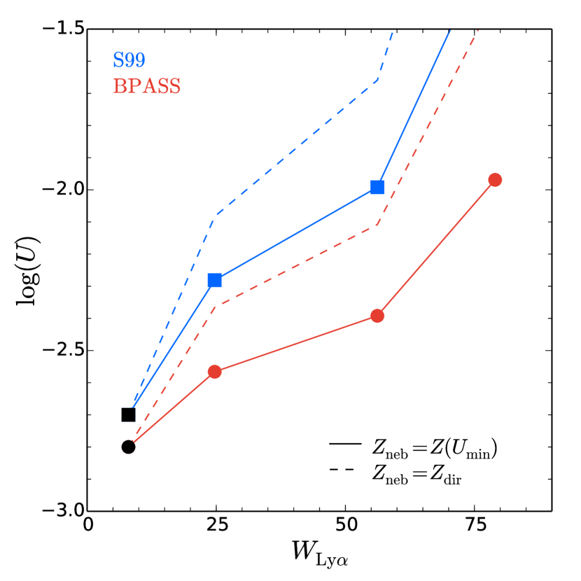
Figure 14.— The ionization parameter $U$ inferred from the composite spectrum of a given galaxy sample vs. the stacked spectroscopic equivalent width $W_{\rm Ly\alpha}$${}_{\textrm{\scriptsize{,spec}}}$ of that sample. Black points refer to the LBG measurements of Steidel et al. (2016), while colored points correspond to the full, low-$W_{\rm Ly\alpha}$, and high-$W_{\rm Ly\alpha}$ LAE samples presented in this paper. Circles and solid red lines indicate the minimum value of $U$ (for any metallicity $0.01\leq Z_{\textrm{\scriptsize{neb}}}/Z_{\odot}\leq 1.0$) consistent with N2 limits and the best-fit measurement of O3 as predicted by the BPASS stellar model. Squares and solid blue lines are the analogous curve for the S99 models, and a linear extrapolation is assumed for log$U>-1.5$. Dashed lines reflect the assumption of $Z_{\textrm{\scriptsize{neb}}}=0.22Z_{\odot}$ for each LAE sample. In general, the differences between the S99 and BPASS models become more apparent as $W_{\rm Ly\alpha}$ increases.

Similarly, the allowed range of $U$ shifts even farther from the S16 measurements for the high-$W_{\rm Ly\alpha}$ sample. Only the most extreme S99 models are able to reproduce O3 line ratios consistent with the high-$W_{\rm Ly\alpha}$ constraints (yellow region in the left panel), and none of the S99 models reproduce the best-fit value for that sample. Even the BPASS models require extremely high ionization parameters (log$U\approx-2.0$) to reproduce the best-fit value of O3 at $W_{\rm Ly\alpha}>57$Å, although values as low as log$U\approx-2.5$ are allowed by the constraining region (which accounts for sample variance in the composite spectrum). Together with the low-$W_{\rm Ly\alpha}$ and full sample of LAEs, the constraints indicate that the characteristic nebular ionization parameter for a population of galaxies grows with the typical Ly$\alpha$ equivalent width among that population.

This trend can be seen more clearly in Fig. 14. Here, we show the minimum value of the ionization parameter $U$ consistent with the best-fit O3 ratio for each of the LAE samples (marginalizing over the gas-phase metallicity) as a function of the median Ly$\alpha$ equivalent width $W_{\rm Ly\alpha}$ of that sample. For comparison, we also include the best-fit value of $U$ from S16 with the measured value of $W_{\rm Ly\alpha}$ from the composite UV LBG spectrum. The minimum $U$ inferred from both the BPASS and S99 $Z_{*}=0.07Z_{\odot}$ models are shown as solid curves. We also include the variation in $U$ assuming the nebular metallicity inferred from the REL-corrected direct method (Sec. 4.2) as dashed curves (although the true metallicity is likely to vary among the $W_{\rm Ly\alpha}$ subsamples). As in Figs. 12 & 13, the increase in $U$ with $W_{\rm Ly\alpha}$ is clearly visible, as is the fact that the softer S99 models require higher values of $U$ to reproduce the observational constraints. In fact, the deviation between the two stellar population models grows with $W_{\rm Ly\alpha}$, indicating that Ly$\alpha$-emitting populations may be particularly advantageous galaxy samples for discriminating among these stellar models. If the high-$W_{\rm Ly\alpha}$ LAEs have lower oxygen abundances than the intermediate and low-$W_{\rm Ly\alpha}$ samples, as might be expected from the BPT-$W_{\rm Ly\alpha}$ relation seen in the LBG sample (Fig. 7), the slope of the $U$-$W_{\rm Ly\alpha}$ relation may be even steeper than displayed in Fig. 14, which has necessarily marginalized over this variation. Conversely, harder stellar spectra resulting from lower iron abundances among high-$W_{\rm Ly\alpha}$ LAEs could reduce the necessary value of $U$. Future observations that probe the ionization state of the gas with less dependence on metallicity (i.e., via O32 or [Ne III]/[O II]) and further cross-checks of the gas-phase oxygen abundance (e.g., from N2) will therefore provide more powerful tests of the physical properties of stars and their surrounding gaseous regions.

6.3. Low metallicity objects

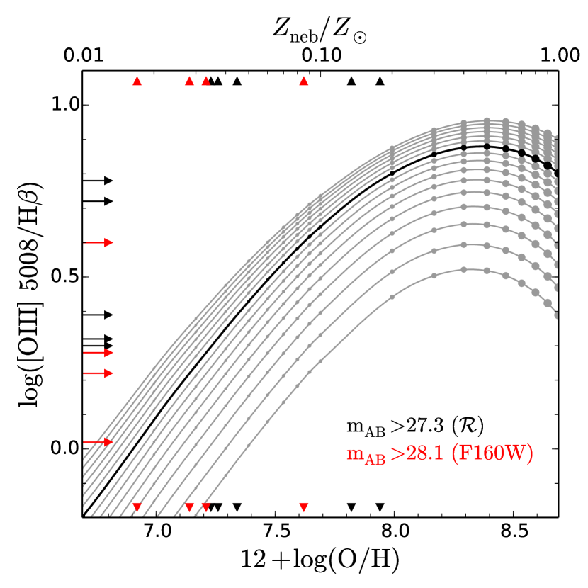
Figure 15.— Inferred oxygen abundances for the faintest LAEs in our sample. Red and black arrows on the left side are the measured O3 ratios for the continuum-undetected LAEs in Fig. 2. These values are converted to abundances (shown as triangles on the top and bottom axes) assuming the log$U=-2.1$ BPASS photoionization model (black curve). Grey curves show the full range of modeled ionization parameters; choosing a higher (lower) log$U$ curve will yield a lower (higher) inferred oxygen abundance at fixed O3.

As shown in Figs. 12 & 13, the relationship between $Z_{\textrm{\scriptsize{neb}}}$ and O3 is double-valued, and its shape at $0.3\lesssim Z_{\textrm{\scriptsize{neb}}}\lesssim 0.9$ makes it very difficult to constrain the gas-phase oxygen abundance from O3 measurements alone. However, at low values of $Z_{\textrm{\scriptsize{neb}}}$, the relationship becomes much steeper, and the abundances of objects that can be assumed to occupy the low-$Z_{\textrm{\scriptsize{neb}}}$ or high-$Z_{\textrm{\scriptsize{neb}}}$ branches may be constrained much more easily.

Fig. 2 shows that the O3 ratios of our individual LAEs exhibit a marked downturn at the lowest continuum luminosities. Based on the photoionization models discussed above, these lower values of O3 could be explained by the faintest LAEs having 1) significantly higher stellar metallicities, 2) lower ionization parameters, and/or 3) lower gas-phase metallicities (i.e., oxygen abundance) compared to the typical LAEs in our sample.

Given the fact that the LAEs exhibit higher ionization parameters than the continuum-bright LBGs and seem to require similar (or lower) stellar metallicities, we suggest that the observed downturn is caused by low oxygen abundances among the faintest LAEs. This interpretation is supported by other arguments as well: Ly$\alpha$-emitting galaxies that are faint at $\lambda_{\textrm{\scriptsize{rest}}}\approx 1900-4500$Å are likely to have low stellar masses and high specific star-formation rates, both qualities that correlate with low oxygen abundances in other galaxy samples. Finally, the shape of the $Z_{\textrm{\scriptsize{neb}}}$$-$O3 relation would predict a sharp downturn, as O3 is fairly flat at $Z_{\textrm{\scriptsize{neb}}}\gtrsim 0.3$ but decreases quickly for $Z_{\textrm{\scriptsize{neb}}}\lesssim 0.2$. As the typical inferred gas-phase metallicity of our LAE sample is $Z_{\textrm{\scriptsize{neb}}}\approx 0.22Z_{\odot}$, we would expect LAEs with below-average oxygen abundances to exhibit significantly lower values of O3.

We therefore interpret the O3 values of the faintest LAEs according to the following assumptions: they have ionization parameters at least as high as that inferred for the typical LAEs in our sample (log$U\approx-2.1$) and have stellar populations similar to the BPASS $Z_{*}=0.07Z_{\odot}$ models that match the LAE and LBG composite spectra discussed above. We also assume that each of these LAEs occupies the lower-metallicity track ($Z_{\textrm{\scriptsize{neb}}}<0.4Z_{\odot}$) where the $Z_{\textrm{\scriptsize{neb}}}$$-$O3 relation is double-valued (this assumption is discussed further below).

Fig. 15 shows the oxygen abundances that are inferred for our 9 continuum-undetected LAEs with measured O3 ratios based on these assumptions. The measured O3 ratios are shown as arrows on the left axis, while the inferred oxygen abundances (nebular metallicities) are shown on the bottom (top) axis. As in Fig. 2, black points are LAEs undetected in our ground-based continuum images ($\mathcal{R}>27.3$), while the red points are also undetected in deep HST images ($m_{\textrm{\scriptsize{AB, F160W}}}>28.1$). The $Z_{\textrm{\scriptsize{neb}}}$$-$O3 curve with log$U=-2.1$ is shown in black (with points as in Figs. 12 & 13), while the analogous curves for other ionization parameters are shown in grey.

The inferred oxygen abundances for the continuum-undetected LAEs are in the range 12 + log(O/H) = $6.9-8.0$, with six LAEs below 12 + log(O/H) = 7.4 ($Z_{\textrm{\scriptsize{neb}}}<0.05Z_{\odot}$). Increasing the assumed ionization parameter would require even lower oxygen abundances to produce the observed values of O3. While some individual objects may have lower ionization parameters than that assumed, we suggest that it is unlikely that the average ionization parameter is significantly lower among these LAEs than the typical LAEs in our sample for the reasons discussed above. We have assumed each of our LAEs occupies the low-metallicity track of the $Z_{\textrm{\scriptsize{neb}}}$$-$O3 curve; for all but two of the continuum-undetected LAEs, the high-metallicity track would predict significantly super-solar average metallicities, which would be extremely suprising for galaxies that otherwise appear to be young, low-mass galaxies.

7. Discussion

The above results indicate that our population of faint LAEs exhibit distinct physical properties with respect to the population of brighter, more massive, and more rapidly star-forming LBGs. In this section we compare these properties to those of other extreme, low-mass galaxy samples, arguing that galaxies selected via emission lines (including Ly$\alpha$) are representative of the low-mass, low-luminosity population. We also discuss the mechanisms by which the nebular properties may be linked to galaxy mass and Ly$\alpha$ production and escape.

7.1. Comparison to other extreme high-$z$ galaxy samples

As discussed in Sec. 1, some recent samples of galaxies selected by their extreme nebular emission lines show similar stellar masses and other properties to the KBSS-Ly$\alpha$ LAEs described here. The three “extreme” LBGs with $T_{e}$ measurements presented by Steidel et al. (2014) have $M_{*}=10^{9.4-9.7}$, SFR = 30$-$60 $\rm M_{\odot}$ yr^-1, and O3 = 0.79$-$0.9. Maseda et al. (2013, 2014) present samples of 14 and 22 EELGs with median dynamical masses $\langle M_{\textrm{\scriptsize{dyn}}}\rangle\approx 10^{9.1}$$\rm M_{\odot}$. This mass is ostensibly similar to that estimated for the KBSS-Ly$\alpha$ LAEs in T15 ($\langle M_{\textrm{\scriptsize{dyn}}}\rangle\approx 10^{8.9}$$\rm M_{\odot}$), but Maseda et al. assume a geometric factor $C\equiv r_{\textrm{\scriptsize{eff}}}\sigma^{2}/GM_{\textrm{\scriptsize{dyn}}}=3$, while T15 assumes $C=5$. A consistent choice of estimator would suggest that the Maseda et al. (2013, 2014) EELGs have dynamical masses $\sim$0.5 dex higher than the LAEs described here. Similarly, the median Maseda et al. (2014) SFR (9 $\rm M_{\odot}$ yr^-1 inferred from SED fitting) is roughly double our median LAE SFR (5 $\rm M_{\odot}$ yr^-1 from dust-corrected H$\alpha$). Masters et al. (2014) present an even higher-SFR sample of EELGs, with average SFR = 29 $\rm M_{\odot}$.

Despite these differences, the EELG samples share many physical properties with the KBSS-Ly$\alpha$ LAEs, including low inferred metallicities. Maseda et al. (2014) calculate oxygen abundances for 7 EELGs from the direct $T_{e}$ method or strong-line indicators, finding 12 + log(O/H) = 7.45$-$8.25 and a median value of 7.90. Masters et al. (2014) find higher typical abundances via the N2 estimator for their EELG sample, with median 12 + log(O/H) = 8.34 and individual values ranging from 8.67 (roughly solar) to $<$7.82. Our derived $T_{e}$ metallicity is consistent with these median values within 1$\sigma$, although neither EELG sample utilizes the +0.24 dex correction we assume for our $T_{e}$ measurement (Sec. 4.2). If we neglect this factor for consistency, then our estimated oxygen abundance 12 + log(O/H) = 7.80$\pm$0.17 is lower than either EELG sample (but still consistent with the Maseda et al. 2014 median within 1$\sigma$). Similarly, our lowest-metallicity objects appear to be at least as low as the individual EELGs, with at least 5 LAEs in our sample having lower metallicities than the lowest EELGs according to our analysis in Sec. 6.3. Masters et al. (2014) observe a turnover in the R23-N2 plane at 12 + log(O/H) $\lesssim$ 8.4, mirroring the turnover seen in the O3 distribution of our faintest LAEs (Figs. 2 & 15). Similarly, Henry et al. (2013) find a downturn in both R23 and O3 at $M_{*}\lesssim 10^{8.8}\rm M_{\odot}$ in a sample of $z\sim 2$ EELGs. This evidence suggests that both the typical and extreme metallicities observed in our LAE sample are at least as low as those measured by other emission-line selections, which is likely consistent with the lower masses and SFRs inferred for our sample, as well as their higher redshifts.

While galaxy selections based on line emission are effective at identifying low-mass, low-metallicity galaxies, it is important to consider whether all such galaxies are selected by this method; only $\sim$50% of $L\sim L_{*}$ LBGs exhibit Ly$\alpha$ in emission (Shapley et al., 2003; Steidel et al., 2010). A relatively unbiased selection of intrinsically-faint galaxies may be achieved through gravitational lensing, which has proven fruitful at selecting galaxies with $L\ll L_{*}$ at $z\approx 1.5-3$ (e.g., Alavi et al. 2014; Stark et al. 2014). Stark et al. (2014) present 17 UV continuum selected gravitationally lensed galaxies with masses $M_{*}\approx 2.0\times 10^{6}-1.4\times 10^{9}$$\rm M_{\odot}$. While not selected based on line emission, these galaxies exhibit emission in many UV metal lines including N IV], O III], C IV, Si III], and C III]. Stark et al. (2014) find that Ly$\alpha$ emission closely tracks the emission of other high-excitation lines such as C III], as was previously seen by Shapley et al. (2003). Furthermore, all 11 galaxies for which Ly$\alpha$ fell within the observed passband exhibited Ly$\alpha$ emission, with 10/11 galaxies having $W_{\rm Ly\alpha}\gtrsim 20$Å. This result is consistent with recent work by Oyarzún et al. (2016), who find that the fraction of Ly$\alpha$ emitters increases as galaxy mass decreases, with $\sim$86% of galaxies with $10^{7.6}<M_{*}/\rm M_{\odot}\leq 10^{8.5}$ at $3<z<4.6$ showing Ly$\alpha$ in emission with a typical equivalent width $W_{\rm Ly\alpha}\approx 36$Å. The high incidence of Ly$\alpha$ emission at low galaxy masses therefore suggests that our sample of faint LAEs is likely to be fairly representative of the total population of faint, low-mass, star-forming galaxies at $z\approx 2-3$.

Stark et al. (2014) also conducted photoionization modeling of the rest-UV emission lines in 4 galaxies from their sample. This subset has inferred stellar masses $10^{7.46}\leq M_{*}/\rm M_{\odot}\leq 10^{8.06}$ and oxygen abundances 7.29 $\leq$ 12 + log(O/H) $\leq$ 7.82 (0.04 $\leq Z/Z_{\odot}\leq$ 0.13). These abundances are similar to those inferred for our faintest LAEs. Stark et al. (2014) find ionization parameters $-2.16\leq$log$U\leq-1.84$ using (single-star) stellar models from Bruzual & Charlot (2003); these values are similar to those inferred for our LAE sample using the S99 models. Based on our analysis in Sec. 6, we expect that Stark et al. (2014) would have inferred lower ionization parameters using stellar models including intrinsically-harder ionizing spectra similar to the BPASS models we employ here (discussed further in Sec. 7.2 below).

Finally, recent rest-optical galaxy photometry at $z=3-7$ has indicated that extreme line emission is ubiquitous in the earliest galaxy populations (e.g., Stark et al. 2013; Schenker et al. 2013; Smit et al. 2014). In particular, Smit et al. (2014) find that bright, lensed galaxies ($M_{\textrm{\scriptsize{UV}}}\approx-20$) at $z\sim 7$ have typical rest-frame equivalent widths of EW([O III]+H$\beta$) $>$ 637Å, including 4 extreme objects with EW $\approx$ 1500Å. The KBSS LAE composite has EW([O III]+H$\beta$) $=$ 829Å, comparable to these high-$z$ samples and significantly higher than the LM1 LBG composite from Steidel et al. (2016), which has EW([O III]+H$\beta$) $=$ 238Å. The 4 LAEs in our sample that are undetected in HST/WFC3 (Fig. 2) require EW([O III]+H$\beta$) $\gtrsim$ 1000$-$1700Å, which mirrors the extreme subsample of Smit et al. (2014) and further indicates the resemblance between the faintest galaxies at $z\approx 2-3$ and their progenitors at the highest redshifts.

In summary, the KBSS-Ly$\alpha$ LAEs presented in this paper appear to have similar nebular properties to the faintest galaxies and most extreme line-emitters selected by other surveys at comparable redshifts (as well as the reionization epoch), although our sample is the first to include a large sample of rest-optical spectra of galaxies in this luminosity and redshift regime.

7.2. Origins of strong line emission in faint galaxies

We now turn our discussion to the physical interpretation of our observations: why is Ly$\alpha$ emission so strongly linked to the nebular line properties and continuum luminosities of galaxies?

The strong nebular line emission of faint galaxies is partially a result of the relationship between mass and metallicity; as discussed above, the low metallicities of low-mass galaxies naturally produce strong emission in many high-excitation nebular lines. However, the connection between Ly$\alpha$ emission and the excitation state of nebular gas is less clear.

One natural explanation of this link may be the shape of the incident stellar spectra that drive the line emission from the nebular gas. Both high excitation (parameterized by the O3 ratio) and high $W_{\rm Ly\alpha}$ are indicators of an intrinsically hard incident spectrum. The intrinsic Ly$\alpha$ luminosity of an ionization-bounded H II region is approximately proportional to the total production of ionizing photons, so $W_{\rm Ly\alpha}$ is a measure of the ratio of ionizing to non-ionizing incident UV flux (modulo the subsequent scattering and absorption of the Ly$\alpha$ photons). Similarly, the O3 ratio is strongly dependent on the shape of the ionizing spectrum, which may be conceptualized as the ratio of $\sim$1$-$2 Ryd photons to $\sim$2$-$4 Ryd photons. Stellar populations that produce high numbers of ionizing photons to non-ionizing photons will typically also produce harder spectra within the hydrogen-ionizing band, which may generate the observed relation.

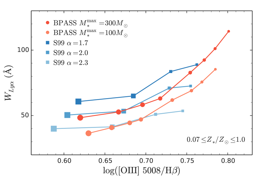
Figure 16.— Predicted $W_{\rm Ly\alpha}$ and O3 ratios from Cloudy photoionization models for BPASS (circles) and S99 (squares) model spectra of varying stellar metallicities ($0.07Z_{\odot}\leq Z_{*}\leq Z_{\odot}$ with symbol size increasing with $Z_{*}$). The predictions are computed for a fiducial nebular metallicity $Z_{\textrm{\scriptsize{neb}}}=0.2Z_{\odot}$ and ionization parameter log$U=-2.1$. We plot multiple IMFs for each model, varying the upper mass cutoff for the BPASS models ($M^{\textrm{\scriptsize{max}}}_{*}=300\rm M_{\odot}$ or $100\rm M_{\odot}$) and the IMF slope for the S99 models ($\alpha=-2.3$, $-2.0$, or $-1.7$). In all cases, the harder stellar spectra produce higher $W_{\rm Ly\alpha}$ and O3 ratios, providing a qualitative explanation for the BPT-Ly$\alpha$ relation and other nebular trends explored in this paper. Notably, however, the standard-IMF S99 models do not produce values of $W_{\rm Ly\alpha}$ consistent with typical LAE measurements.

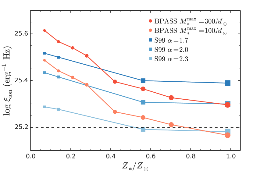
Figure 17.— Predicted $\xi_{\textrm{\scriptsize{ion}}}$ ratios for the same BPASS and S99 model spectra presented in Fig. 16. The same low-metallicity stellar models that produce acceptable fits to the N2-BPT and $W_{\rm Ly\alpha}$ constraints (i.e., the BPASS models) likewise predict $\xi_{\textrm{\scriptsize{ion}}}$ ratios significantly higher than the “canonical” values assumed by typical models of reionization (e.g., Robertson et al. 2015; dashed line at log$(\xi_{\textrm{\scriptsize{ion}}}/[\mathrm{erg}^{-1}\mathrm{Hz}])=25.2$). These stellar models therefore naturally produce high ionization parameters and reduce the requirements for ubiquitously high LyC escape fractions among primeval galaxies.

We provide an example of the above argument using photoionization models in Fig. 16. For each of the stellar models, we consider a variety of stellar metallicities and IMF parameters, but the general relation remains the same: models that produce high O3 ratios likewise predict high intrinsic values of $W_{\rm Ly\alpha}$. The trend is especially clear for the BPASS models, for which the stellar metallicity strongly modulates the total ionizing photon production (Fig. 17) and thereby the secondary production of Ly$\alpha$ photons.

The parameter $\xi_{\textrm{\scriptsize{ion}}}$ is defined as the number of hydrogen-ionizing photons produced by a stellar population per unit UV luminosity (typically normalized at 1500Å). A value log($\xi_{\textrm{\scriptsize{ion}}}/$erg^-1 Hz) = 25.2 has been assumed by recent work modeling reionization (e.g., Robertson et al. 2013, 2015), which is appropriate for a single-star population with a typical IMF in steady-state (e.g., the $\alpha=2.3$ S99 model in Fig.  17). The BPASS models produce much higher values of $\xi_{\textrm{\scriptsize{ion}}}$ at low metallicity, even with the the same IMF ($M_{*}^{\textrm{\scriptsize{max}}}=100\rm M_{\odot}$). Because reionization constraints impose a requirement on the total galactic emission of ionizing photons, which is proportional to $\xi_{\textrm{\scriptsize{ion}}}\times f_{\textrm{\scriptsize{esc,LyC}}}$, these models therefore reduce the global LyC escape fraction required to reionize the Universe (e.g., Ma et al. 2016).

In addition, these high values of $\xi_{\textrm{\scriptsize{ion}}}$ also provide a natural explanation for the high ionization parameters inferred for our LAE sample. At fixed gas density, the ionization parameter $U$ is proportional to the number density of ionizing photons. While the expected value of $U$ in high-$z$ H II regions may not be obvious a priori, a variation of $\sim$0.7 dex (as appears to be present between the LBG and LAE samples; Fig. 12) would be extremely difficult to explain without a significant difference in $\xi_{\textrm{\scriptsize{ion}}}$ between the two populations. While a very young stellar population age could elevate $\xi_{\textrm{\scriptsize{ion}}}$ in individual galaxies, our measurements of high $U$ for a large sample of LAEs–and their correspondence to typical galaxies in their mass and luminosity range, as argued above–suggests that these faint galaxies efficiently produce large numbers of ionizing photons in steady state.

The strong dependence of $\xi_{\textrm{\scriptsize{ion}}}$ on $Z_{*}$ among the BPASS models provides an alternative mechanism to modulate the ionization parameter. Sanders et al. (2016) identify an anti-correlation between gas-phase metallicity and $U$ among continuum-selected galaxies from the MOSDEF survey. The similar trend seen here among the KBSS LAEs and LBGs which may indicate that the effect of metallicity on the hardness of the stellar spectra drives the large observed variation in $U$ with galaxy luminosity.

Lastly, as discussed in Sec. 6.2, the hardness of the ionizing field and the ionization parameter produce somewhat degenerate effects on the nebular excitation (O3): the softer S99 models require significantly higher values of $U$ to produce the same values of the O3 ratio. By this token, both the normalization and the shape of the BPASS ionizing spectra are favorable for high nebular excitation. Firstly, their intrinsic hardness can produce high O3 with values of $U$ that are only moderately elevated with respect to more luminous populations. Secondly, their high $\xi_{\textrm{\scriptsize{ion}}}$ values at low metallicities naturally produce the large total number of ionizing photons required explain these $U$ values at apparently fixed gas density.

To summarize, invoking a stellar population model in which the spectra become significantly harder at low metallicities (whether via the specific BPASS model suite or a set of similar output model spectra) will self-consistently reproduce the strong Ly$\alpha$ and nebular line ratios observed for faint, high-redshift galaxies.

7.3. Ly$\alpha$ emission and LyC leakage

As discussed in Sec. 5.2.2, there are indications that Ly$\alpha$-emitting galaxies have elevated O32 ratios with respect to typical galaxies. Some studies have suggested that these ratios are indicative of density-bounded H II regions, in which the entire star-forming cloud becomes ionized. Such regions would be expected to lack a partially-ionized boundary wherein low-ionization species may dominate the local line emission and thereby lower the luminosity-averaged measurement of the ionization ratio (see discussion by e.g., Jaskot & Oey 2013; Nakajima et al. 2013; Nakajima & Ouchi 2014). Some evidence for this behavior is seen in local observations of H II regions using the ionization parameter mapping technique (IPM; Pellegrini et al. 2012; Zastrow et al. 2013). In particular, the IPM measurements of the Large Magellanic Cloud by Pellegrini et al. (2012) indicate that optically-thick H II regions are surrounded by ionization fronts that are dominated by low-ionization species (e.g., high [S II]/[S III] ratios), whereas optically-thin (i.e., density-bounded) regions are dominated by high-ionization species throughout. As an illustrative example of this phenomenon, Fig. 18 reproduces the results of a Cloudy photoionization simulation in which a slab of gas with a variable, uniform column density is illuminated by a BPASS model spectrum. In the density-bounded case (optically thin at the Lyman limit; $\tau_{912}\ll 1$), the O32 ratio is elevated by $\sim$0.6 dex with respect to the ionization-bounded case ($\tau_{912}\gg 1$).

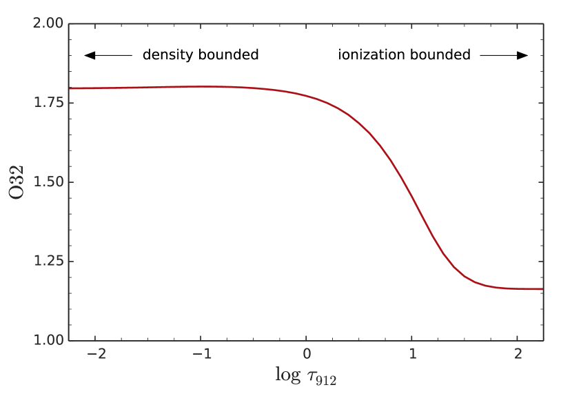
Figure 18.— Predicted O32 ratios from Cloudy photoionization models for a plane-parallel slab of gas with varying total optical depth at the Lyman limit ($\tau_{912}$). Incident radiation field is that of the BPASS $Z_{*}=0.07Z_{\odot}$ model, with log$U=-2.1$ and $Z_{\textrm{\scriptsize{neb}}}=0.2$ as in the preceding figures. Optically thin (that is, density-bounded; $\tau_{912}\lesssim 1$) ionized regions are characterized by elevated O32 ratios.

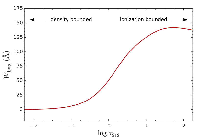
Figure 19.— Predicted $W_{\rm Ly\alpha}$ ratio for the same photoionization models presented in Fig. 18. Optically-thin ionized regions produce little Ly$\alpha$ emission, which peaks at column densities of H I that are moderately optically thick to ionizing photons. Note that the Cloudy photonization code is not optimized to reproduce the behavior of $W_{\rm Ly\alpha}$ at the highest values of $\tau_{912}$, where Ly$\alpha$ transmission is dominated by resonant scattering in a dusty medium.

Such density-bounded regions are highly interesting for studies of EoR galaxies because they produce large local escape fractions of ionizing photons (and potentially of Ly$\alpha$ photons, although Ly$\alpha$ production may be suppressed; Fig. 19). There are observational indications that galaxies with high O32 ratios are more likely to leak ionizing (LyC) photons: several recently-discovered LyC leakers at low-redshift (Izotov et al., 2016a, b) show high ionization states (O32 $>0.6$). However, these galaxies were selected as likely LyC emitters based on these same nebular line ratios, and other low-$z$ LyC leakers show smaller values of O32 (Leitet et al., 2013; Borthakur et al., 2014; Leitherer et al., 2016). At $z\sim 3$, two confirmed LyC leakers are known: Ion2 (de Barros et al., 2016) and Q1549-C25 (Shapley et al., 2016). Ion2 was selected based on broadband continuum colors according to the method of Vanzella et al. (2015) and is associated with extreme line ratios (O32 $>$ 1 & EW${}_{\textrm{\scriptsize{rest}}}$([O III]) = 1500Å; Vanzella et al. 2016). Conversely, Q1549-C25 appears to have more moderate line emission (EW${}_{\textrm{\scriptsize{rest}}}$([O III]+H$\beta$) = 256Å) typical of KBSS LBGs.

Given the diversity of known LyC-leakers, is unclear that real high-$z$ density-bounded H II regions must necessarily have high O32 ratios. Harder ionizing photons have smaller ionization cross-sections and longer mean free paths than lower-energy photons, which could cause H II regions to become hotter and more highly ionized at large radii. This effect may be stronger at high redshift, where we have argued that low-metallicity stellar populations are likely to produce hard ionizing spectra. In addition, any dominance of low-ionization species within ionization fronts of individual H II regions need not translate to a low O32 ratio in the luminosity-weighted, galaxy-averaged observations conducted for distant galaxies.

Furthermore, Ly$\alpha$ production is extremely weak in H II regions with uniformly low gas column densities (Fig. 19). In more realistic simulations of Ly$\alpha$ production and escape in a clumpy, multi-phase ISM, Dijkstra et al. (2016) find that both ionizing and Ly$\alpha$ photons escape through low-column-density sightlines, in agreement with observational indicators that a patchy distribution of gas is required for efficient photon escape. In T15, we found that the escape fraction of Ly$\alpha$ photons was significantly related to a galaxy’s covering fraction of neutral (or low-ionization) gas. Similarly, the low-$z$ LyC leaker discovered by Borthakur et al. (2014) has a very low value of O32 $=-0.5$, but also exhibits a low covering fraction of low-ionization gas. Photons may also be scattered or extinguished far from their original H II regions; Steidel et al. (2011) found that star-forming galaxies emit Ly$\alpha$ radiation at large radii even when they appear to be Ly$\alpha$ absorbers in slit spectroscopy. However, the galaxies with high spatially-integrated values of $W_{\rm Ly\alpha}$ are those with centrally-concentrated Ly$\alpha$ emission, suggesting that the bulk of Ly$\alpha$ (and potentially LyC) absorption occurs at small galactocentric radii.

Together, these observations indicate that the distribution of H I gas on many spatial scales plays a strong role in scattering and extinguishing Lyman radiation, a fact which likely produces much of the scatter in the relationships between $W_{\rm Ly\alpha}$ and nebular properties explored in Secs. 5$-$6. Nonetheless, both the nebular properties of the KBSS-Ly$\alpha$ LAEs and their neutral gas distributions presented in T15 indicate that they are strong candidates for Lyman-continuum leakage and ideal analogs of EoR galaxies.

8. Conclusions

In this paper, we have shown that the Ly$\alpha$-emitting properties of galaxies (including 60 faint LAEs and 368 brighter LBGs) are closely linked to the properties of their embedded star-forming regions, as probed by rest-optical and rest-UV spectroscopy. This sample of galaxies from the KBSS and KBSS-Ly$\alpha$ represents the largest set of combined Ly$\alpha$ and nebular-line spectroscopy of galaxies at any redshift and spans a large range of galaxy properties, including luminosities, SFRs, masses, extinctions, ionization states, and net Ly$\alpha$ emission.

By constructing composite spectra from our LAE sample, we also set new constraints on the physical properties of $L\approx 0.1L_{*}$ galaxies at $z\approx 2-3$. The primary conclusions of this work are summarized below:

1. Faint LAEs have extremely high nebular excitation (parameterized by the [O III] $\lambda$5008/H$\beta$ ratio) consistent with most extreme LBGs in current surveys, which are likely the low-metallicity tail of the galaxy distribution. Fig. 5; Sec. 4

2. A 2.8$\sigma$ detection of the [O III] $\lambda$4364 auroral emission line suggests that the H II regions in these LAEs have high electron temperatures with respect to more massive LBGs ($T_{\textrm{\scriptsize{$e$,LAE}}}=1.78\pm 0.33\times 10^{4}$K). Calculating a metallicity via the “direct” ($T_{e}$) method gives a typical LAE oxygen abundance of 12 + log(O/H) = 8.04$\pm$0.19 ($Z_{\textrm{\scriptsize{neb}}}=0.22^{+0.12}_{-0.08}Z_{\odot}$) after correcting for the $-$0.24 dex offset of metallicities derived from this collisionally-ionized transition. This metallicity is consistent with our limits from the O3N2 and N2 strong-line indicators. Fig. 6; Secs. 4.2$-$4.3

3. The continuum-faintest LAEs in our sample show evidence for the turnover in the [O III] $\lambda$5008/H$\beta$ ratio that occurs at very low metallicities, and six LAEs appear to have oxygen abundances 12 + log(O/H) $\approx$ 6.9$-$7.4 ($Z_{\textrm{\scriptsize{neb}}}\approx 0.02-0.05$). Figs. 2 & 15; Sec. 6.3

4. Across a broad range of LBG and LAE Ly$\alpha$ emissivities, the locations of galaxies in the N2-BPT plane vary systematically with Ly$\alpha$ equivalent width. We find that the variation of dust attenuation with metallicity plays a minor role in this relation, but the ionization and excitation state of the star-forming regions are much more strongly correlated with the net Ly$\alpha$ emission. In particular, the photoionization models of the LAEs require ionization parameters log$U\approx-2.1$ for typical LAEs, 0.7 dex higher than typical LBGs. Figs. 7$-$14; Sec. 5

5. The rest-frame optical spectra of the KBSS-Ly$\alpha$ LAEs indicate stellar populations that produce harder spectra than typical stellar population models. Successful stellar models include those with very low stellar metallicities (which are consistent with the low Fe/O abundances reported elsewhere), and those that include the effects of binary interaction on the evolution of massive stars. In particular, we are unable to reproduce the properties of the highest-$W_{\rm Ly\alpha}$ LAEs except with stellar models that include binary evolution. Figs. 12$-$14; Sec. 6

6. In general, the nebular properties of faint LAEs at $z\approx 2-3$ indicate the production and escape of large numbers of ionizing photons, which we argue is typical of low-luminosity galaxies at high redshift. Combined with our previous work indicating the low covering fraction of neutral gas around these faint galaxies, we suggest that analogous galaxies at $z\gtrsim 6$ may be more effective at reionizing the Universe than is typically assumed in current models. Figs. 16$-$19; Sec. 7

Future work will include measuring additional global properties of these galaxies, including the variation of nebular excitation and Ly$\alpha$ production with the physical sizes, masses, and star-formation rates of individual LAEs. Additional indicators of the nebular properties (including ionization state and strong-line metallicity indicators) will provide valuable cross-checks of the measurements inferred here. In a few years, JWST will be able to obtain similar spectra of $L\sim 0.1L_{*}$ galaxies without being limited by ground-based atmospheric windows, facilitating further analysis of the variation of these galaxy properties across populations and redshifts.

References

- Abazajian et al. (2009) Abazajian, K. N., Adelman-McCarthy, J. K., Agüeros, M. A., et al. 2009, ApJS, 182, 543
- Alavi et al. (2014) Alavi, A., Siana, B., Richard, J., et al. 2014, ApJ, 780, 143
- Aller (1984) Aller, L. H., ed. 1984, Astrophysics and Space Science Library, Vol. 112, Physics of thermal gaseous nebulae
- Amorín et al. (2012) Amorín, R., Pérez-Montero, E., Vílchez, J. M., & Papaderos, P. 2012, ApJ, 749, 185
- Andrews & Martini (2013) Andrews, B. H., & Martini, P. 2013, ApJ, 765, 140
- Asplund et al. (2009) Asplund, M., Grevesse, N., Sauval, A. J., & Scott, P. 2009, ARA&A, 47, 481
- Baldwin et al. (1981) Baldwin, J. A., Phillips, M. M., & Terlevich, R. 1981, PASP, 93, 5
- Berg et al. (2015) Berg, D. A., Skillman, E. D., Croxall, K. V., et al. 2015, ApJ, 806, 16
- Borthakur et al. (2014) Borthakur, S., Heckman, T. M., Leitherer, C., & Overzier, R. A. 2014, Science, 346, 216
- Bresolin et al. (2016) Bresolin, F., Kudritzki, R.-P., Urbaneja, M. A., et al. 2016, ArXiv e-prints, arXiv:1607.06840
- Brinchmann et al. (2008) Brinchmann, J., Pettini, M., & Charlot, S. 2008, MNRAS, 385, 769
- Brocklehurst (1971) Brocklehurst, M. 1971, MNRAS, 153, 471
- Brott et al. (2011) Brott, I., de Mink, S. E., Cantiello, M., et al. 2011, A&A, 530, A115
- Brown et al. (2014) Brown, J. S., Croxall, K. V., & Pogge, R. W. 2014, ApJ, 792, 140
- Bruzual & Charlot (2003) Bruzual, G., & Charlot, S. 2003, MNRAS, 344, 1000
- Campbell et al. (1986) Campbell, A., Terlevich, R., & Melnick, J. 1986, MNRAS, 223, 811
- Cardamone et al. (2009) Cardamone, C., Schawinski, K., Sarzi, M., et al. 2009, MNRAS, 399, 1191
- Cardelli et al. (1989) Cardelli, J. A., Clayton, G. C., & Mathis, J. S. 1989, ApJ, 345, 245
- de Barros et al. (2016) de Barros, S., Vanzella, E., Amorín, R., et al. 2016, A&A, 585, A51
- Dijkstra et al. (2016) Dijkstra, M., Gronke, M., & Venkatesan, A. 2016, ArXiv e-prints, arXiv:1604.08208
- Dopita et al. (2000) Dopita, M. A., Kewley, L. J., Heisler, C. A., & Sutherland, R. S. 2000, ApJ, 542, 224
- Eldridge & Stanway (2009) Eldridge, J. J., & Stanway, E. R. 2009, MNRAS, 400, 1019
- Eldridge & Stanway (2016) —. 2016, ArXiv e-prints, arXiv:1602.03790
- Erb et al. (2016) Erb, D. K., Pettini, M., Steidel, C. C., et al. 2016, ArXiv e-prints, arXiv:1605.04919
- Erb et al. (2006) Erb, D. K., Shapley, A. E., Pettini, M., et al. 2006, ApJ, 644, 813
- Esteban et al. (2014) Esteban, C., García-Rojas, J., Carigi, L., et al. 2014, MNRAS, 443, 624
- Ferland et al. (2013) Ferland, G. J., Porter, R. L., van Hoof, P. A. M., et al. 2013, Revista Mexicana de Astronomía y Astrofísica, 49, 137
- Finkelstein et al. (2011) Finkelstein, S. L., Hill, G. J., Gebhardt, K., et al. 2011, ApJ, 729, 140
- Garnett (1992) Garnett, D. R. 1992, AJ, 103, 1330
- Gawiser et al. (2006) Gawiser, E., van Dokkum, P. G., Gronwall, C., et al. 2006, ApJ, 642, L13
- Hagen et al. (2014) Hagen, A., Ciardullo, R., Gronwall, C., et al. 2014, ApJ, 786, 59
- Hagen et al. (2016) Hagen, A., Zeimann, G. R., Behrens, C., et al. 2016, ApJ, 817, 79
- Henry et al. (2015) Henry, A., Scarlata, C., Martin, C. L., & Erb, D. 2015, ArXiv e-prints, arXiv:1505.05149
- Henry et al. (2013) Henry, A., Scarlata, C., Domínguez, A., et al. 2013, ApJ, 776, L27
- Hopkins et al. (2014) Hopkins, P. F., Kereš, D., Oñorbe, J., et al. 2014, MNRAS, 445, 581
- Izotov et al. (2016a) Izotov, Y. I., Orlitová, I., Schaerer, D., et al. 2016a, Nature, 529, 178
- Izotov et al. (2016b) Izotov, Y. I., Schaerer, D., Thuan, T. X., et al. 2016b, ArXiv e-prints, arXiv:1605.05160
- Izotov et al. (2006) Izotov, Y. I., Stasińska, G., Meynet, G., Guseva, N. G., & Thuan, T. X. 2006, A&A, 448, 955
- Jaskot & Oey (2013) Jaskot, A. E., & Oey, M. S. 2013, ApJ, 766, 91
- Kennicutt (1998) Kennicutt, Jr., R. C. 1998, ARA&A, 36, 189
- Kewley et al. (2013) Kewley, L. J., Dopita, M. A., Leitherer, C., et al. 2013, ApJ, 774, 100
- Kewley et al. (2001) Kewley, L. J., Dopita, M. A., Sutherland, R. S., Heisler, C. A., & Trevena, J. 2001, ApJ, 556, 121
- Kornei et al. (2010) Kornei, K. A., Shapley, A. E., Erb, D. K., et al. 2010, ApJ, 711, 693
- Kriek et al. (2015) Kriek, M., Shapley, A. E., Reddy, N. A., et al. 2015, ApJS, 218, 15
- Kroupa (2001) Kroupa, P. 2001, MNRAS, 322, 231
- Leitet et al. (2013) Leitet, E., Bergvall, N., Hayes, M., Linné, S., & Zackrisson, E. 2013, A&A, 553, A106
- Leitherer et al. (2014) Leitherer, C., Ekström, S., Meynet, G., et al. 2014, ApJS, 212, 14
- Leitherer et al. (2016) Leitherer, C., Hernandez, S., Lee, J. C., & Oey, M. S. 2016, ApJ, 823, 64
- Levesque et al. (2012) Levesque, E. M., Leitherer, C., Ekstrom, S., Meynet, G., & Schaerer, D. 2012, ApJ, 751, 67
- Liu et al. (2008) Liu, X., Shapley, A. E., Coil, A. L., Brinchmann, J., & Ma, C.-P. 2008, ApJ, 678, 758
- Ma et al. (2016) Ma, X., Hopkins, P. F., Kasen, D., et al. 2016, ArXiv e-prints, arXiv:1601.07559
- Ma et al. (2015) Ma, X., Kasen, D., Hopkins, P. F., et al. 2015, MNRAS, 453, 960
- Maseda et al. (2013) Maseda, M. V., van der Wel, A., da Cunha, E., et al. 2013, ApJ, 778, L22
- Maseda et al. (2014) Maseda, M. V., van der Wel, A., Rix, H.-W., et al. 2014, ApJ, 791, 17
- Masters et al. (2016) Masters, D., Faisst, A., & Capak, P. 2016, ArXiv e-prints, arXiv:1605.04314
- Masters et al. (2014) Masters, D., McCarthy, P., Siana, B., et al. 2014, ApJ, 785, 153
- Matthee et al. (2016) Matthee, J., Sobral, D., Oteo, I., et al. 2016, MNRAS, 458, 449
- McLean et al. (2010) McLean, I. S., Steidel, C. C., Epps, H., et al. 2010, in Society of Photo-Optical Instrumentation Engineers (SPIE) Conference Series, Vol. 7735, Society of Photo-Optical Instrumentation Engineers (SPIE) Conference Series
- McLean et al. (2012) McLean, I. S., Steidel, C. C., Epps, H. W., et al. 2012, in Society of Photo-Optical Instrumentation Engineers (SPIE) Conference Series, Vol. 8446, Society of Photo-Optical Instrumentation Engineers (SPIE) Conference Series
- McLinden et al. (2011) McLinden, E. M., Finkelstein, S. L., Rhoads, J. E., et al. 2011, ApJ, 730, 136
- Momose et al. (2014) Momose, R., Ouchi, M., Nakajima, K., et al. 2014, MNRAS, 442, 110
- Nakajima & Ouchi (2014) Nakajima, K., & Ouchi, M. 2014, MNRAS, 442, 900
- Nakajima et al. (2013) Nakajima, K., Ouchi, M., Shimasaku, K., et al. 2013, ApJ, 769, 3
- Oke et al. (1995) Oke, J. B., Cohen, J. G., Carr, M., et al. 1995, PASP, 107, 375
- Ono et al. (2012) Ono, Y., Ouchi, M., Mobasher, B., et al. 2012, ApJ, 744, 83
- Osterbrock & Ferland (2006) Osterbrock, D. E., & Ferland, G. J. 2006, Astrophysics of gaseous nebulae and active galactic nuclei
- Oteo et al. (2015) Oteo, I., Sobral, D., Ivison, R. J., et al. 2015, MNRAS, 452, 2018
- Oyarzún et al. (2016) Oyarzún, G. A., Blanc, G. A., González, V., et al. 2016, ApJ, 821, L14
- Pellegrini et al. (2012) Pellegrini, E. W., Oey, M. S., Winkler, P. F., et al. 2012, ApJ, 755, 40
- Pentericci et al. (2011) Pentericci, L., Fontana, A., Vanzella, E., et al. 2011, ApJ, 743, 132
- Pettini & Pagel (2004) Pettini, M., & Pagel, B. E. J. 2004, MNRAS, 348, L59
- Pilyugin et al. (2012) Pilyugin, L. S., Grebel, E. K., & Mattsson, L. 2012, MNRAS, 424, 2316
- Pilyugin et al. (2009) Pilyugin, L. S., Mattsson, L., Vílchez, J. M., & Cedrés, B. 2009, MNRAS, 398, 485
- Price et al. (2014) Price, S. H., Kriek, M., Brammer, G. B., et al. 2014, ApJ, 788, 86
- Reddy et al. (2008) Reddy, N. A., Steidel, C. C., Pettini, M., et al. 2008, ApJS, 175, 48
- Robertson et al. (2015) Robertson, B. E., Ellis, R. S., Furlanetto, S. R., & Dunlop, J. S. 2015, ApJ, 802, L19
- Robertson et al. (2013) Robertson, B. E., Furlanetto, S. R., Schneider, E., et al. 2013, ApJ, 768, 71
- Rudie et al. (2012) Rudie, G. C., Steidel, C. C., Trainor, R. F., et al. 2012, ApJ, 750, 67
- Salpeter (1955) Salpeter, E. E. 1955, ApJ, 121, 161
- Sana et al. (2012) Sana, H., de Mink, S. E., de Koter, A., et al. 2012, Science, 337, 444
- Sanders et al. (2015) Sanders, R. L., Shapley, A. E., Kriek, M., et al. 2015, ApJ, 799, 138
- Sanders et al. (2016) —. 2016, ApJ, 816, 23
- Schenker et al. (2013) Schenker, M. A., Ellis, R. S., Konidaris, N. P., & Stark, D. P. 2013, ApJ, 777, 67
- Schenker et al. (2014) —. 2014, ApJ, 795, 20
- Schenker et al. (2012) Schenker, M. A., Stark, D. P., Ellis, R. S., et al. 2012, ApJ, 744, 179
- Shapley et al. (2005) Shapley, A. E., Steidel, C. C., Erb, D. K., et al. 2005, ApJ, 626, 698
- Shapley et al. (2003) Shapley, A. E., Steidel, C. C., Pettini, M., & Adelberger, K. L. 2003, ApJ, 588, 65
- Shapley et al. (2016) Shapley, A. E., Steidel, C. C., Strom, A. L., et al. 2016, ApJ, 826, L24
- Shapley et al. (2015) Shapley, A. E., Reddy, N. A., Kriek, M., et al. 2015, ApJ, 801, 88
- Sharples et al. (2013) Sharples, R., Bender, R., Agudo Berbel, A., et al. 2013, The Messenger, 151, 21
- Smit et al. (2014) Smit, R., Bouwens, R. J., Labbé, I., et al. 2014, ApJ, 784, 58
- Song et al. (2014) Song, M., Finkelstein, S. L., Gebhardt, K., et al. 2014, ApJ, 791, 3
- Stanway et al. (2016) Stanway, E. R., Eldridge, J. J., & Becker, G. D. 2016, MNRAS, 456, 485
- Stark et al. (2010) Stark, D. P., Ellis, R. S., Chiu, K., Ouchi, M., & Bunker, A. 2010, MNRAS, 408, 1628
- Stark et al. (2011) Stark, D. P., Ellis, R. S., & Ouchi, M. 2011, ApJ, 728, L2
- Stark et al. (2013) Stark, D. P., Schenker, M. A., Ellis, R., et al. 2013, ApJ, 763, 129
- Stark et al. (2014) Stark, D. P., Richard, J., Siana, B., et al. 2014, MNRAS, 445, 3200
- Steidel et al. (2011) Steidel, C. C., Bogosavljević, M., Shapley, A. E., et al. 2011, ApJ, 736, 160
- Steidel et al. (2010) Steidel, C. C., Erb, D. K., Shapley, A. E., et al. 2010, ApJ, 717, 289
- Steidel et al. (2004) Steidel, C. C., Shapley, A. E., Pettini, M., et al. 2004, ApJ, 604, 534
- Steidel et al. (2016) Steidel, C. C., Strom, A. L., Pettini, M., et al. 2016, ArXiv e-prints, arXiv:1605.07186
- Steidel et al. (2014) Steidel, C. C., Rudie, G. C., Strom, A. L., et al. 2014, ApJ, 795, 165
- Strom et al. (2016) Strom, A. L., Steidel, C. C., Rudie, G. C., et al. 2016, ArXiv e-prints, arXiv:1608.02587
- Trainor & Steidel (2013) Trainor, R., & Steidel, C. C. 2013, ApJ, 775, L3
- Trainor & Steidel (2012) Trainor, R. F., & Steidel, C. C. 2012, ApJ, 752, 39
- Trainor et al. (2015) Trainor, R. F., Steidel, C. C., Strom, A. L., & Rudie, G. C. 2015, ApJ, 809, 89
- Vanzella et al. (2015) Vanzella, E., de Barros, S., Castellano, M., et al. 2015, A&A, 576, A116
- Vanzella et al. (2016) Vanzella, E., de Barros, S., Vasei, K., et al. 2016, ArXiv e-prints, arXiv:1602.00688
- Yajima et al. (2014) Yajima, H., Li, Y., Zhu, Q., et al. 2014, MNRAS, 440, 776
- Zastrow et al. (2013) Zastrow, J., Oey, M. S., Veilleux, S., & McDonald, M. 2013, ApJ, 779, 76