Quasi-optical theory of microwave plasma heating in open magnetic trap
Abstract
Microwave heating of a high-temperature plasma confined in a large-scale open magnetic trap, including all important wave effects like diffraction, absorption, dispersion and wave beam aberrations, is described for the first time within the first-principle technique based on consistent Maxwell’s equations. With this purpose, the quasi-optical approach is generalized over weakly inhomogeneous gyrotrotropic media with resonant absorption and spatial dispersion, and a new form of the integral quasi-optical equation is proposed. An effective numerical technique for this equation’s solution is developed and realized in a new code QOOT, which is verified with the simulations of realistic electron cyclotron heating scenarios at the Gas Dynamic Trap at the Budker Institute of Nuclear Physics (Novosibirsk, Russia).
I Introduction
The absorption of electromagnetic waves under the electron cyclotron resonance (ECR) conditions is widely used for heating of high-temperature plasmas in toroidal magnetic traps (tokamaks and stellarators). However, for many years the use of this method in open magnetic configurations has been limited either by plasma heating in relatively compact laboratory installationsV16 , or by MHD stabilization of low-density plasmaV13 ; V14 ; V15 . The only exception was the TMX-U experiment at Lawrence Livermore National Laboratory where electron temperatures up to 0.28 keV were obtained with ECR heating, but these studies were concluded soonV12 . And only recently an efficient ECR heating of a dense (comparable to toroidal devices) plasma has been demonstrated at a large-scale mirror trap. We mean successful experiments on a combined plasma heating by neutral beams and microwave radiation performed at the Gas Dynamic Trap (GDT) device in the Budker Institute of Nuclear PhysicsX7 ; X8 ; X9 ; X10 . In particular, direct and highly-localized heating of the thermal electron component allows to achieve the GDT experiment the record for open traps electron temperature of 1 keV at the plasma axisX8 . These studies convincingly demonstrate good prospects for the use of simple axially symmetric open magnetic traps as a powerful source neutron for fusion applications Simonen .
Implementing the effective ECR heating of a dense plasma at a large open trap requires a revision of the prevailing ideas about the physics of cyclotron absorption as well as the subsequent transport of energy and MHD stabilization of a plasma column. None of the well-understood techniques developed for the toroidal plasma heating works well in this case X4 . Numerical modeling of the propagation and absorption of electromagnetic waves in an inhomogeneous plasma plays an important role in this occasion. Until recently, such modeling was only possible in the framework of the geometric optics approximation also known as ray-tracing. In particular, the basic ECR heating scenario used in the GDT has been originally proposed and justified with the ray-tracing calculations X4 ; X5 ; X6 . However, in this scenario there are areas of reflection and strong absorption of waves, in which the medium is not smooth as compared to a wavelength. So, detailed understanding of the involved processes requires to go beyond the geometric optics approximation.
The main effects that violate the geometric optics are associated with the spatial dispersion in a strongly inhomogeneous region of resonant absorption, the diffraction of a wave beam, and the caustic formation in the vicinity of internal reflection points of a wave beam. Straightforward simulation of these effects for large devices within a complete set of Maxwell’s equations is very complicated, in particular, because of the smallness of a wavelength. A good alternative is the consistent quasi-optical approach based on an asymptotic expansion of Maxwell’s equations in the paraxial approximation in the vicinity of the selected Wentzel–Kramers–Brillouin (WKB) mode Balakin_2007a ; fullQOp2 .
In this paper, the quasi-optical approximation is adopted to describe the propagation of wave beams in a high-temperature plasma in an open magnetic trap. A similar approach was previously developed for toroidal magnetic traps Balakin_2008 ; BECCD . However, description of the microwave heating in modern open traps needs substantial modification of the quasi-optical theory due to a requirement of more accurate accounting of the spatial dispersion inside the resonant absorption zone. The physics of this difference originates from the fact that the magnetic field in open configuration typically changes along its direction, while in the toroidal geometry the magnetic field varies presumably in orthogonal direction. As a result, the factorizing approach to the quasi-optical Hamiltonian, that works well in the modeling of wave propagation in a toroidal trap, fails completely in case of a large open trap. This motivates us to find a new, more general and accurate, non-factorized formulation of the theory resulted in the substantial modification of a numerical algorithm, which eventually led to development of an entirely new code.
The remainder of this paper is organized as follows: Sec. II derives the basic equations of quasi-optical approximation and their applicability conditions; Sec. III defines a general ansatz for a dielectric response of inhomogeneous dispersive media and derive the quasi-optical evolution operator; peculiarities related to wave dissipation are considered, and modification of the dissipative part of the early defined evolution operator is proposed in Sec. IV; a numerical method for solving the quasi-optical equation is developed in Sec. V; the model is adopted to a particular case of hot magnetized plasmas confined in an open magnetic trap in Sec. VI; first results of simulations of real scenarios of ECR plasma heating at the GDT device are discussed in Sec. VII; and Sec. VIII summarizes the results.
II Basic quasi-optical equation
A rigorous derivation of the quasi-optical approximation for a weakly inhomogeneous gyrotropic and anisotropic media with spatial dispersion may be found in Refs. fullQOp1, ; fullQOp2, . The main steps are described below. Let us start with Maxwell’s equations for processes written in the ‘‘operator’’ form
| (1) |
where a summation over double indexes is implied. The operator acts on -th Cartesian component of the electric field vector, is the vacuum wave number, is the wave number operator defined as the differentiation in the coordinate space, and is the linear operator obtained from the dielectric tensor by a formal substitution ,
The latter operation is not uniquely defined because and do not commute; in the next section we describe the ‘‘best way’’ of regularizing the expression for providing that the kernel is known. The result may be expressed in terms of Fourier-integral:
| (2) |
For the smoothly inhomogeneous medium, the approximate solution of Maxwell’s equations can naturally be found in the form of quasi-optical beam corresponding to some chosen WKB mode. To do this, we define the polarization vector for the interested WKB mode as a solution of algebraic Maxwell’s equations in a locally homogeneous medium. Next, using the same technique as in the transition , the polarization vector can be associated with the polarization operator . Then, the approximate solution of Eq. (1) can be found in the following form
Here, the polarization operator acts on the scalar amplitude of the wave beam. The equation for takes the form
| (3) |
Note that the corresponding function
is usually used as a ray Hamiltonian in the geometrical optics. Similar, we will call the operator as a quasi-optical Hamiltonian.
Presently, we consider axisymmetric open traps and magnetic configurations with weakly broken axial symmetry. In this case, we can use either Cartesian coordinate system or a cylindrical coordinate system with the polar axis aligned along the trap axis. Let us introduce the coordinates and the canonically conjugated momenta as
| (4) |
where is the coordinate along the trap axis, is the set of two coordinates in the transverse plane, and .
Assuming the smoothness of beam parameters along , we can introduce the scalar amplitude of in the form
where is the complex envelope of a wave beam, and function defines the dependence of the ‘‘carrier phase’’ of the wave field along the axis. Substituting this field in Eq. (3), we obtain the equation for the envelope as
| (5) |
In contrast to geometrical optics, here we have certain freedom in the choice of related to the phase variation over the transverse aperture of the wave beam. After several tries, we found that the most convenient and reliable way in numerical calculations is to define as a solution to a local dispersion equation with transverse wave vector corresponding to the center of mass of a wave spectrum in the cross-section :
where is the center of mass for a wave field in the cross-section .
Assuming the complex envelope to be a smooth function on the longitudinal coordinate, , we expand Eq. (5) to the first order in powers of (or, equivalently, in powers of ):
| (6) |
where , i.e. it is with omitted derivatives over . With the limit of geometrical optics, the last term in Eq. (6) results in a pre-exponential factor responsible for the variation of the wave amplitude due the effect of ‘‘group’’ slowing down. This term may be eliminated with formal substitution
As a result, we obtain a more simple equation
| (7) |
This is our basic equation that describes the evolution of the scalar wave beam amplitude along -axis, including the effects of diffraction, spatial dispersion and dissipation, as long as condition of the paraxial approximation holds. Except few very special cases, operator is local, i.e. it may be approximated with multiplication by known function as long as the media is smooth compared to the wave length. In this case, the new amplitude is also defined by local transformation .
The simple form of Eq. (7) suggests a clear physical interpretation of the evolution operator . Indeed, this is a longitudinal wave number expressed as a function of the transverse wave vector in an operator form:
| (8) |
Below we will show how to restore this operator from the WKB-solution of an algebraic dispersion relation in a locally homogeneous medium.
Our approach may be adopted to highly curved magnetic configurations, e.g. typical for radiation belts in Earth ionosphere or Solar flares, in a straightforward manner—just by introducing new coordinates with a curvilinear axis and taking into account the curvature when calculating a conjugated momenta operator. The similar approach was previously used for toroidal magnetic traps in which the axis was chosen along the reference geometric optics ray representing the center of the quasi-optical wave beam Balakin_2007a ; Balakin_2008 ; BECCD . However, using geometric optics rays as a reference for the quasi-optical equation in open traps is not optimal because such rays may be strongly curved and even divergent inside the plasma column in most interesting cases X4 ; X9 .
III Evolution operator
The main difficulty in the practical use of the quasi-optical equation (7) is the uncertainty of the dielectric permittivity operator , which is necessary for definition of the evolution operator . Obviously, the operator for any inhomogeneous linear media can be generated by some kernel function , and such kernel can be introduced in infinite different ways. The most optimal (for our needs) way is proposed in quite rigorous manner in Ref. operator, , where the dielectric operator is represented as
| (9) |
Here . For such operator, a Hermitian kernel, , always generates a Hermitian operator in a sense of natural scalar product . Correspondingly, an anti-Hermitian kernel, , generates an anti-Hermitian operator. This important non-trivial feature allows to preserve the energy conservation law when constructing the dielectric response of inhomogeneous media. The kernel function is obtained as the sum of the amendments to the dielectric permittivity tensor over the powers of characteristic inhomogeneity scale :
As a reasonable approximation in a smoothly inhomogeneous media with , one can only account the lowest term, , which is indeed the dielectric permittivity tensor obtained for a ‘‘locally homogeneous’’ media, i.e. in the geometric optics approximation.
To find a Fourier representation, let us substitute
into Eq. (9). Then
Noting that summation over is just a Taylor series for we obtain Eq. (2). It should be stressed that expressions (2) and (9) remain valid for any kernel , and for every linear inhomogeneous problem such kernel exists. The problem is, however, that except some trivial model cases, see e.g. Ref. operator, , this kernel is known only with the accuracy provided by geometric optics.
The dielectric permittivity operator unambiguously defines the evolution operator in Eq. (7). However, we can cut the computations and obtain the same result by just noting that the evolution operator may be found essentially in the same way as the dielectric operator . So, the operator is generated by the scalar function
| (10) |
and as a practical approximation to in a weakly inhomogeneous media, one can use a solution of the locally homogeneous problem. The only difference we should have in mind is that coordinate is a parameter here—there is no differentiation over in operator , therefore instead of 6-dimensional phase-space we use 4-dimensional space . Due to the term , the evolutionary operator (10) becomes local either in real space for an inhomogeneous medium without spatial dispersion with , or in -space for a homogeneous dispersive medium with , or for combination . The latter has been used in simulations for toroidal configurations Balakin_2008 ; BECCD , but we find this approximation being not suitable for open traps. Thus, we must deal with a general form below.
As already mentioned, symmetric form of the integral representation allows to introduce the dielectric response of an inhomogeneous medium that is compatible with the energy conservation. In the present context, Eq. (10) always results in Hermitian operators for real kernel and anti-Hermitian operators for purely imaginary . However, this feature is insufficient to provide a correct description of inhomogeneous dissipative medium with spatial dispersion. As shown in the next section, equation (10) may give absurd results and, therefore, needs modification.
IV Dissipative correction
Let us decompose the linear operator over Hermitian and anti-Hermitian parts
where and are both Hermitian operators in the sense of the standard scalar product . It can be shown that with the same accuracy as Eq. (7), is proportional to the total wave energy flux in the cross-section . Then, using the quasi-optical equation (7) one can find the linear density of the absorbed power as
| (11) |
Hermitian operator in Eq. (7) conserves the energy flux, thus describing non-dissipative medium. As expected, the anti-Hermitian part of the evolution operator is responsible for the dissipation or pumping of the wave field.
From the geometric optics limit, we know that energy dissipation corresponds to a positive sign of . Let us now consider the eigenvalues of the ‘‘dissipative’’ operator with the dissipative kernel according to Eq. (10). One may expect that all , however this is not true. Procedure (10) guarantees only since is Hermitian, but not the positive sign of . In particular, we had negative with a first try to apply Eq. (10) to model the resonant wave absorption in magnetized plasma.
Fortunately, we have found a simple practical way to correct the evolution operator, which guarantees a definite sign of . To do this, we define a square of some other Hermitian operator:
| (12) |
where operator is constructed similar to Eq. (10) but with kernel
New operator provides the same WKB limit as the old one. If the operator kernel is defined within the geometric optics approximation, then formal difference between both operators is of higher order than their accuracy. The modified quasi-optical equation (7) then takes the following form
| (13) |
The discussed problem of the absorbed power in an inhomogeneous medium with spatial dispersion may be illustrated with a simple one-dimensional example. Consider the following Hamiltonian kernel with positive imaginary part
Corresponding non-modified evolution operator (10) is
According to Eq. (11), the absorbed power density along the axis is
The r.h.s. of this expression does not conserve the sign. For example, the Gaussian wave beam corresponds to
In particular, non-shifted beam with , regardless of its width , always results in a negative absorbed power. Shifted beam with propagates without dissipation. These strange solutions disappear for modified evolution operator (12). In this case
and the absorbed power density of the new operator possesses a positive sign:
Note that the dissipation-free solution is still present, but in this case it corresponds to unbounded distribution with an infinite power flux.
V Numerical solution
The linear integro-differential equation (7) involves time consuming integration in 4-dimensional space . Therefore, an algorithm economic both in calculation of the r.h.s. and in number of -steps is of major importance. We develop such algorithm having in mind essential features of a beam propagation physics in resonant dispersive media.
As a starting point one can consider an explicit scheme in which a small but finite integration step over the evolution coordinate is defined as
where
| (14) |
This is a generalization of the operator exponent technique studied in Refs. Balakin_2008, ; Fraiman95, . One can find that this scheme results in an exact solution with any finite either for a homogeneous dispersive medium, , or for an inhomogeneous medium without spatial dispersion, . For a general case of a dispersive inhomogeneous medium, , this scheme converges to the exact solution for .
The operator exponent method is rigorously justified only for dissipation-free media described by a Hermitian evolution operator. In this case, there is the effective numerical scheme for calculating the operator (14) requiring no more than operations with being the number of mesh points in 2-dimensional space . In contrast to the traditional finite difference methods Samarsky , there are no formal limitations on the step imposed by grid size in . Although the scheme is explicit, the integration step is limited only by physical ‘‘inhomogeneities’’ of a medium, namely, by the value of commutator between and :
| (15) |
However, operator (14) may result in a solution with an exponentially growing energy in inhomogeneous dissipative media. One of the reasons, already described in the previous section, is that the dissipation in terms of geometric optics, , does not guarantee the positive-definiteness of the corresponding operator term . More generally, this is a known issue of finding a proper approximation for physically correct wave absorption in media with a spatial dispersionGinz ; Brambilla ; TokWest1 ; TokWest2 ; TokWest3 ; Balakin_diss . In our case, errors in the approximation of the Hermitian part (e.g. numerical errors due to violation of condition (15)) disturb only the wave beam phase, therefore, their influence is manifested over the large diffraction length. On the contrary, errors in the approximation of the anti-Hermitian part directly affect the beam amplitude, resulting in the worst case in an exponential grows of an error. Our experience tells that this problem is especially actual for microwave beams in the electron cyclotron frequency range, when the resonant dissipation varies dramatically both in coordinate and wave vectors spaces.
These problems are essentially solved with the modification of anti-Hermitian part of the evolution operator suggested with Eq. (12). For numerical solving of the corresponding quasi-optical equation (13), we propose to use the ‘‘split-step’’ method, i.e. the sequential solutions for the separate Hermitian and anti-Hermitian parts. The integration step is then
with is an approximation to the operator exponent of the Hermitian part, it is given by Eq. (14) with . Opposite to the Hermitian part, the dissipation operator does not fit the form suitable for an efficient computation of the operator exponent (just because it requires two iterations of ). Calculation of the operator exponent in this case requires about number of steps, where is an eigenvalue of matrix , which is typically too much for practical applications. Another way is to compute approximately by using conventional methods such as Adams or Runge–Kutta Samarsky . Such calculations are also very time demanding, mainly because of large eigenvalues that may appear after a double iteration of and the need to reduce the integration step to provide a numerical stability.
On the other hand, large positive eigenvalues correspond to quickly damped or even evanescent modes that typically do not represent physical interest. This makes it possible to replace the operator exponent with some approximate operator , which correctly describes all weakly damped modes and ensures exponential decay for heavily damped and non-propagating modes with large eigenvalues. To fulfill the first condition we require that both operators have the same asymptotic behavior at :
To ensure that the second requirement, it is sufficient to ‘‘cut’’ the integral kernel of at large . The simplest operator satisfying the above conditions is
| (16) |
where operator is constructed similar to Eq. (10) but with kernel
is an arbitrary one-dimensional function with the following properties: when , and for . In our code we use the hyperbolic tangent . Calculation of the operator (16) reduces to a consistent application of the Fourier transform to the factorized kernel, so the computational complexity for is only by a factor of two greater than that for .
VI Description of hot magnetized plasma in open magnetic trap
In this section, we define the kernel for quasi-optical evolution operator used in the numerical simulation of microwave plasma heating in open magnetic trap. Our model is based on the dispersion relation for electromagnetic waves propagating in a locally homogeneous hot magnetized plasma with Maxwellian distribution functions. This approach is justified for modern experiments in which the microwave energy is deposited into relatively dense plasma. Exactly in this case the electrodynamic quasi-optical effects become important, while the kinetic effects related to the rf-driven modification of the electron distribution function are not essential. For example, the Maxwellian distribution formed during ECR heating of bulk electrons was proved at the GDT device by direct laser scattering measurementsX8 ; X9 ; X10 . Kinetic effects are important in the opposite case of low density plasma, such as GAMMA-10 experimentV14 or ECR assisted start-up at the GDTYack2016 , in which electrodynamics is usually well described by standard geometric optics or beam tracing, but dielectric response of non-Maxwellian electrons is calculated self-consistently by means of a quasi-linear Fokker–Planck codeFP1 .
In a vicinity of the fundamental electron cyclotron harmonic the dispersion relation of the Maxwellian plasma can be represented as follows tensor :
| (18) |
where and are parallel and perpendicular components of the index of refraction with respect to the external magnetic field, ,
and are standard Stix parameters that determine the plasma density and the strength of the confining magnetic field through, respectively, Langmuir and cyclotron frequencies of electrons, is the normalized thermal velocity for electrons. All effects associated with the spatial dispersion and resonant dissipation at the fundamental harmonic are defined in the ‘‘warm’’ part in by so-called plasma dispersion function Brambilla
with argument . These formulas are obtained for a weakly relativistic plasma , a small Larmor radius , and a quasi-longitudinal wave propagation that allows omitting the relativistic resonance broadening compared to the non-relativistic Doppler shift. These conditions are definitely met, at least, in current experiments at the GDT device.
Having in mind applications to a long and axially symmetric devices, such as GDT, in the current implementation of the code we consider the external magnetic field directed along the trap axis . This simplifies the recovery of the quasi-optical Hamiltonian from the dispersion equation (18), however this assumption is not essential for our technique and may be bypassed if necessary.
For strictly longitudinal magnetic field, the quasi-optical variables (4) are mapped to Stix variables as , . With this substitution, for each point in the real space and each transverse momentum we determine a complex solution of the local dispersion relation (18). Away from the EC resonance this solution is close to the roots of the biquadratic dispersion relation corresponding to a cold plasma limit, . This allows us to choose the ‘‘right’’ root, matching the studied electromagnetic mode, and use it as a starting point for an iterative search for solution of the transcendent equation (18). Additional control for the right choice of the mode is provided by requirement of a smoothness of over , in case of occasional sharp jumps we use the values at neighboring grid cells to recover the correct mode.
Following Eq. (8), the complex kernel of the evolution operator may be defined as
| (19) |
where is the carrier wave vector that corresponds to centers of mass for the wave field distribution and its spectrum in the cross-section ,
Another problem specific for magnetic plasma confinement, is evaluation how the absorbed microwave power is distributed over a trap volume. Here one should keep in mind that this power rapidly redistributes over the magnetic flux surfaces. In this case, the most relevant characteristic of the power deposition is a one-dimensional distribution over the magnetic surfaces, usually referred to as a power deposition profile. This distribution may be found taking into account Eq. (11), as
| (20) |
where the integral is taken over the whole volume occupied by a wave beam, equation defines the magnetic surface, without arguments is the label of a magnetic surface,
is the effective perimeter of a magnetic surface at some fixed cross-section , for an axially symmetric magnetic configuration .
The code QOOT (Quasi-Optics for Open Traps) is developed to solve the quasi-optical equation (13) with iterative procedure (17) for the evolutionary operator defined by kernel (19). The code calculates the power deposition profile (20) in the geometry of an open magnetic trap and visualizes the results. We use the Cartesian coordinates for the wave amplitudes and output of the results, and the internal cylindrical coordinates for the Hamiltonian taking advantage of the axial symmetry of the plasma configuration. As mentioned in the introduction, the development is based on our previous quasi-optical code LAQO, created for toroidal magnetic traps Balakin_2008 . However, since conditions for the wave propagation in open mirror traps and toroidal traps are significantly different, we have eventually developed an entirely new code.

VII Simulation of ECR plasma heating at the GDT device
The basic ECR heating scheme at the GDT relies on radiation trapping by a non-uniform plasma column X4 . This effect is caused by a dependence of the plasma refraction of the magnetic field strength. The radiation is launched through a side of the plasma column at a high magnetic field (close to the magnetic mirror). As a microwave beam propagates in plasma in the direction of the trap center, the magnitude of the magnetic field decreases resulting in conditions for an internal reflection from the plasma-vacuum boundary. The plasma column acts as kind of waveguide, heterogeneous in both transverse and longitudinal directions, whereby the radiation is delivered to the ECR surface. The geometric optics may not be valid in the vicinity of the wave reflection surface due to caustic formation, and near ECR surface due to sharp inhomogeneous damping of the wave field. This casts doubt on the applicability of geometrical optics approximation.
Therefore, the first task for the quasi-optical code is to check our previous results obtained with ray-tracing. In particular, we repeated simulations aimed at optimization of the ECR heating efficiency at the GDT conditions. Previously, it has been found that the efficient ECR heating can be achieved in two distinguished regimes characterized by very different distributions of the absorbed microwave power X9 ; X10 . Switching between these regimes, as well as a fine-tuning of the microwave power deposition profile can be controlled, at specific conditions of the GDT experiment, by a relatively small adjustment of the external magnetic field in the close proximity of the EC resonance.
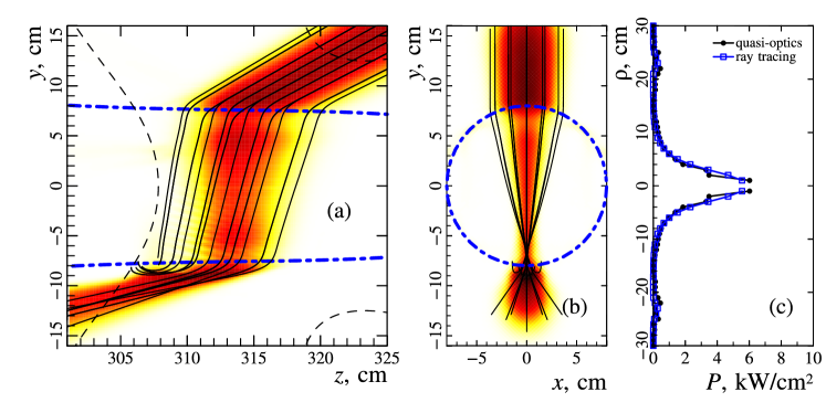
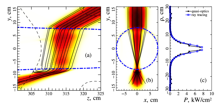
The results are shown in Figures 1–5. For two-dimensional visualization of a quasi-optical beam in plane (face view along the trap axis) and plane (side view) we use the wave intensity integrated along the and axis, correspondingly:
Here characterizes the density of the energy flux along the axis, and projects that flux to the direction of the the group velocity . In explicit form
To improve the contrast, the logarithmic color scale is used corresponding to the levels of , which allowed us to visualize the wave field in caustics. The power deposition profiles are calculated using Eq. (20), applied at the central cross-section where the confining magnetic field has its minimum.
Figures 1 and 2 show the results of simulation, the wave beams and the power deposition profiles, in the ‘‘narrow power deposition’’ regime. In this regime the record values of the electron temperature (up to 1 keV) have been achieved in the GDT experiments. First and second figures correspond, respectively, to states before and after the ECR heating modeled for the experimentally measured plasma density and electron temperature profiles. For comparison, we show the ray-tracing results. In this case, the power deposition profiles obtained by two different methods coincide quite well. Some discrepancy is observed on the periphery of the plasma column. This corresponds to the absorption of radiation after reflection in the vicinity of the caustic surface where geometric optics is violated (caustics are indicated as crossing of neighboring ray trajectories). Note, that the geometric optics rays reproduce the quasi-optical beam satisfactorily both before and inside the caustic region.
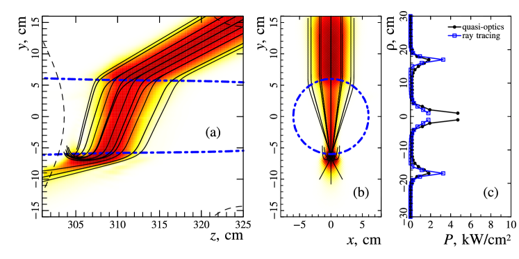
Figures 3 and 4 show the same plots for the ‘‘broad power deposition profile’’ regime. In the experiments in this mode, we observe a pronounced increase of a total plasma energy related to an improved confinement of the hot ions. There is a better agreement between the quasi-optical and geometro-optical power deposition profiles since the ratio of microwave power deposited in the vicinity of the caustic is much lower. As well as the ray-tracing, the quasi-optical simulations predict incomplete absorption of the microwave power in this regime.
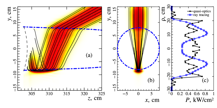
Figure 5 shows predictions for the new regime with ‘‘improved broad power deposition’’. This mode has not been yet demonstrated experimentally; its implementation will be eventually possible after up-grade of the mirror magnetic coil of the GDT system which is currently on progress. All plots correspond to the stage before the microwave heating because the experimental data on plasma profiles after the heating is not available. In this mode, an extended region of the caustic is formed, and the ratio of the power deposition after the caustic is much higher than in the regimes discussed previously. Therefore, the power deposition profiles predicted by the quasi-optics and the ray-tracing vary considerably. We are aware that the quasi-optical modeling provides a more adequate description, but confirmation of this statement requires further studies and experiments, the results of which will be published separately.
Finally, it can be concluded that geometric optics seems to be a reasonable agreement with the more accurate quasi-optical simulations for the most heating scenarios that are already realized in the GDT experiment. However, this conclusion does not exclude a possible impact of spatial dispersion on the resonance dissipation and of diffraction losses near the caustic surfaces in future experiments with more optimized heating scenarios.
VIII Summary
The quasi-optical model of propagation of wave beams in high-temperature magnetically confined plasmas, developed earlier for toroidal traps, is generalized over open magnetic systems. The specifics of microwave heating in modern open traps require substantial improvement of the early quasi-optical theory, associated with more accurate description of the effects of spatial dispersion in the region of resonant wave dissipation. As a result, a new form for the quasi-optical equation is proposed, see Eq. (13). Basing on this equation the universal code QOOT is developed for simulation of electron cyclotron plasma heating, which allows to resolve the diffraction, dispersion and aberration effects in the propagation and absorption of electromagnetic wave beams in open traps.
The code is used to verify the results of optimizing the efficiency of the ECR heating in the large mirror trap GDT, previously obtained by using ray-tracing within geometric optics approximation. First quasi-optical simulations justify the possibility to control the radial distribution of the deposited microwave power by local modification of the magnetic field in near the EC resonance and, in particular, the ability of effective on-axis heating the electron component at the GDT conditions. The influence of wave caustics on a localization of the deposited microwave power is demonstrated.
Acknowledgements.
This work was supported by the Russian Science Foundation (grant No 14-12-01007). The authors would like to thank Dr. Alexander Solomakhin from the Budker Institute for his support with magnetic configurations and ray-tracing modeling for the GDT.References
- (1) A.V. Vodopyanov, S.V. Golubev, V.G. Zorin, A.Yu. Kryachko, A.Ya. Lopatin, V.I. Luchin, S.V. Razin, and A.N. Smirnov, Tech. Phys. Lett. 26(12), 1075 (2000).
- (2) T. Cho, V. P. Pastukhov, W. Horton, T. Numakura, M. Hirata, J. Kohagura, N. V. Chudin, and J. Pratt, Phys. Plasmas 15, 056120 (2008).
- (3) T. Tamano, Phys. Plasmas 2, 2321 (1995).
- (4) T. Saito, K. Ishii, A. Itakura, M. Ichimura, Md. K. Islam, I. Katanuma, J. Kohagura, Y. Tatematsu, Y. Nakashima, T. Numakura, H. Higaki, M. Hirata, H. Hojo, M. Yoshikawa, K. Sakamoto, T. Imai, T. Cho, and S. Miyoshi, J. Plasma Fusion Res. 81(4), 288 (2005).
- (5) T. C. Simonen and R. Horton, Nucl. Fusion 29, 1373 (1989).
- (6) P.A. Bagryansky, Yu.V. Kovalenko, V.Ya. Savkin, A.L. Solomakhin, and D.V. Yakovlev, Nuclear Fusion 54, 082001 (2014).
- (7) P.A. Bagryansky, A.G. Shalashov, E.D. Gospodchikov, A.A. Lizunov, V.V. Maximov, V.V. Prikhodko, E.I. Soldatkina, A.L. Solomakhin, and D.V. Yakovlev, Physical Review Letters 114, 205001 (2015).
- (8) P.A. Bagryansky, E.D. Gospodchikov, Yu.V. Kovalenko, A.A. Lizunov, V.V. Maximov, S.V. Murakhtin, E.I. Pinzhenin, V.V. Prikhodko, V.Ya. Savkin, A.G. Shalashov, E.I. Soldatkina, A.L. Solomakhin, and D.V. Yakovlev, Fusion Science and Technology 68, 87 (2015).
- (9) P.A. Bagryansky, A.V. Anikeev, G.G. Denisov, E.D. Gospodchikov, A.A. Ivanov, A.A. Lizunov, Yu.V. Kovalenko, V.I. Malygin, V.V. Maximov, O.A. Korobeinikova, S.V. Murakhtin, E.I. Pinzhenin, V.V. Prikhodko, V.Ya. Savkin, A.G. Shalashov, O.B. Smolyakova, E.I. Soldatkina, A.L. Solomakhin, D.V. Yakovlev, and K.V. Zaytsev, Nuclear Fusion 55, 053009 (2015).
- (10) T.C. Simonen, Journal of Fusion Energy 35, 63 (2016).
- (11) A. Shalashov, E. Gospodchikov, O. Smolyakova, P. Bagryansky, V. Malygin, and M. Thumm, Physics of Plasmas 19, 052503 (2012).
- (12) А. G. Shalashov, E. D. Gospodchikov, O. B. Smolyakova, P.A. Bagryansky, V. I. Malygin, and M. Thumm, Problems of Atomic Science and Technology, Series: Plasma Physics 6, 49 (2012).
- (13) P.A. Bagryansky, S.P. Demin, E.D. Gospodchikov, Yu.V. Kovalenko, V. I. Malygin, S.V. Murakhtin, V.Ya. Savkin, A.G. Shalashov, O.B. Smolyakov, A.L. Solomakhin, M. Thumm, and D.V. Yakovlev. Fusion Science and Technology 63, no 1T, 40 (2013).
- (14) A.A. Balakin, Radiophysics and Quantum Electronics 55, 502 (2012).
- (15) A.A. Balakin, M.A. Balakina, A.I. Smirnov, and G.V. Permitin, Plasma Phys. Reports 33, 302 (2007).
- (16) A.A. Balakin, M.A. Balakina, and E. Westerhof, Nuclear Fusion 48, 065003 (2008).
- (17) N. Bertelli , A.A. Balakin, E. Westerhof, and M.N. Buyanova, Nucl. Fusion 50, 115008 (2010).
- (18) A.A. Balakin, Radiophysics and Quantum Electronics 55, 472 (2012).
- (19) A.A. Balakin and E.D. Gospodchikov, Journal of Physics B: Atomic, Molecular and Optical Physics 48, 215701 (2015).
- (20) G.M. Fraiman, E.M. Sher, A.D. Yunakovsky, and W.Laedke, Physica D. 87, 325 (1995).
- (21) W.H. Press, S.A. Teukolsky, W.T. Vetterling, and B.P. Flannery, Numerical Recipes: The Art of Scientific Computing (Cambridge University Press, 2007).
- (22) A.A. Balakin, M.A. Balakina, A.I. Smirnov, and G.V. Permitin, Plasma Phys. Reports 34, 533 (2008).
- (23) M. Brambilla, Kinetic Theory of Plasma Waves: Homogeneous Plasmas (Clarendon Press, Oxford, 1998).
- (24) V.L.Ginzburg, Propagation of electromagnetic waves in plasma (Pergamon Press, 1970).
- (25) M.D. Tokman, E. Westerhof, and M.A. Gavrilova, Plasma Phys. and Contr. Fusion 42, 91 (2000).
- (26) M.D. Tokman, E. Westerhof, and M.A. Gavrilova, Journal of Experimental and Theoretical Physics 91(6) 1141 (2000).
- (27) M. D. Tokman, E. Westerhof, and M.A. Gavrilova, Nuclear Fusion, 43, 1295 (2003).
- (28) A.G. Shalashov, A.A. Balakin, E.D. Gospodchikov, T.A. Khusainov, and A.L. Solomakhin, Quasi-optical description microwave plasma heating, accepted by JETP, 2016.
- (29) D. V. Yakovlev, A. G. Shalashov, P. A. Bagryansky, E. D. Gospodchikov, V. Ya. Savkin, and A. L. Solomakhin. Electron-cyclotron plasma startup in the GDT experiment. ArXiv:1607.01051 [physics.plasm-ph] (accepted by Nucl. Fusion, 2016).
- (30) B.W. Stallard, Y. Matsuda and W.M. Nevins, Nucl. Fusion 23(2), 213-223 (1983).
- (31) E. D. Gospodchikov and E. V. Suvorov, Radiophysics and Quantum Electronics 48 (8), 641 (2005).