Type Inference for Static Compilation of JavaScript (Extended Version)

Abstract

We present a type system and inference algorithm for a rich subset of JavaScript equipped with objects, structural subtyping, prototype inheritance, and first-class methods. The type system supports abstract and recursive objects, and is expressive enough to accommodate several standard benchmarks with only minor workarounds. The invariants enforced by the types enable an ahead-of-time compiler to carry out optimizations typically beyond the reach of static compilers for dynamic languages. Unlike previous inference techniques for prototype inheritance, our algorithm uses a combination of lower and upper bound propagation to infer types and discover type errors in all code, including uninvoked functions. The inference is expressed in a simple constraint language, designed to leverage off-the-shelf fixed point solvers. We prove soundness for both the type system and inference algorithm. An experimental evaluation showed that the inference is powerful, handling the aforementioned benchmarks with no manual type annotation, and that the inferred types enable effective static compilation.

1 Introduction

JavaScript is one of the most popular programming languages currently in use red . It has become the de facto standard in web programming, and its growing use in large-scale, real-world applications—ranging from servers to embedded devices—has sparked significant interest in JavaScript-focused program analyses and type systems in both the academic research community and in industry.

In this paper, we report on a type inference algorithm for JavaScript developed as part of a larger, ongoing effort to enable type-based ahead-of-time compilation of JavaScript programs. Ahead-of-time compilation has the potential to enable lighter-weight execution, compared to runtimes that rely on just-in-time optimizations jsC ; v [8], without compromising performance. This is particularly relevant for resource-constrained devices such as mobile phones where both performance and memory footprint are important. Types are key to doing effective optimizations in an ahead-of-time compiler.

JavaScript is famously dynamic; for example, it contains eval for runtime code generation and supports introspective behavior, features that are at odds with static compilation. Ahead-of-time compilation of unrestricted JavaScript is not our goal. Rather, our goal is to compile a subset that is rich enough for idiomatic use by JavaScript developers. Although JavaScript code that uses highly dynamic features does exist Richards et al. [2010], data shows that the majority of application code does not require that flexibility. With growing interest in using JavaScript across a range of devices, including resource-constrained devices, it is important to examine the tradeoff between language flexibility and the cost of implementation.

The JavaScript compilation scenario imposes several desiderata for a type system. First, the types must be sound, so they can be relied upon for compiler transformations. Second, the types must impose enough restrictions to allow the compiler to generate code with good, predictable performance for core language constructs (Section 2.1 discusses some of these optimizations). At the same time, the system must be expressive enough to type check idiomatic coding patterns and make porting of mostly-type-safe JavaScript code easy. Finally, in keeping with the nature of the language, as well as to ease porting of existing code, we desire powerful type inference. To meet developer expectations, the inference must infer types and discover type errors in all code, including uninvoked functions from libraries or code under development.

No existing work on JavaScript type systems and inference meets our needs entirely. Among the recently developed type systems, TypeScript typ and Flow flo both have rich type systems that focus on programmer productivity at the expense of soundness. TypeScript relies heavily on programmer annotations to be effective, and both treat inherited properties too imprecisely for efficient code generation. Defensive JavaScript Bhargavan et al. [2013] has a sound type system and type inference, and Safe TypeScript Rastogi et al. [2015] extends TypeScript with a sound type system, but neither supports prototype inheritance. TAJS Jensen et al. [2009] is sound and handles prototype inheritance precisely, but it does not compute types for uninvoked functions; the classic work on type inference for Self Agesen et al. [1993] has the same drawback. Choi et al. Choi et al. [2015b] present a JavaScript type system targeting ahead-of-time compilation that forms the basis of our type system, but their work does not have inference and instead relies on programmer annotations. See Section 6 for further discussion of related work.

This paper presents a type system and inference algorithm for a rich subset of JavaScript that achieves our goals. Our type system builds upon that of Choi et al. Choi et al. [2015b], adding support for abstract objects, first-class methods, and recursive objects, each of which we found crucial for handling real-world JavaScript idioms; we prove these extensions sound. The type system supports a number of additional features such as polymorphic arrays, operator overloading, and intersection types in manually-written interface descriptors for library code, which is important for building GUI applications.

Our type inference technique builds on existing literature (e.g., cois Pottier [2001]; Agesen et al. [1993]; Rastogi et al. [2012]) to handle a complex combination of language features, including structural subtyping, prototype inheritance, first-class methods, and recursive types; we are unaware of any single previous type inference technique that soundly handles these features in combination.

We formulate type inference as a constraint satisfaction problem over a language composed primarily of subtype constraints over standard row variables. Our formulation shows that various aspects of the type system, including source-level subtyping, prototype inheritance, and attaching methods to objects, can all be reduced to these simple subtype constraints. Our constraint solving algorithm first computes lower and upper bounds of type variables through a propagation phase (amenable to the use of efficient, off-the-shelf fixed-point solvers), followed by a straightforward error-checking and ascription phase. Our use of both lower and upper bounds enables type inference and error checking for uninvoked functions, unlike previous inference techniques supporting prototype inheritance Jensen et al. [2009]; Agesen et al. [1993]. As shown in Section 2.3, sound inference for our type system is non-trivial, particularly for uninvoked functions; we prove that our inference algorithm is sound.

Leveraging inferred types, we have built a backend that compiles type-checked JavaScript programs to optimized native binaries for both PCs and mobile devices. We have compiled slightly-modified versions of six of the Octane benchmarks Oct , which ranged from 230 to 1300 LOC, using our compiler. The modifications needed for the programs to type check were minor (see Section 5 for details).

Preliminary data suggests that for resource-constrained devices, trading off some language flexibility for static compilation is a compelling proposition. With ahead-of-time compilation (AOTC), the six Octane programs incurred a significantly smaller memory footprint compared to running the same JavaScript sources with a just-in-time optimizing engine. The execution performance is not as fast as JIT engines when the programs run for a large number of iterations, but is acceptable otherwise, and vastly better than a non-optimizing interpreter (details in Section 5).

We have also created six GUI-based applications for the Tizen tiz platform, reworking from existing web applications; these programs ranged between 250 to 1000 lines of code. In all cases, all types in the user-written JavaScript code were inferred, and no explicit annotations were required. We do require annotated signatures of library functions, and we have created these for many of the JavaScript standard libraries as well as for the Tizen platform API. Experiences with and limitations of our system are discussed in Section 5.

Contributions:

• We present a type system, significantly extending previous work Choi et al. [2015b], for typing common JavaScript inheritance patterns, and we prove the type system sound. Our system strikes a useful balance between allowing common coding patterns and enabling ahead-of-time compilation.

• We present an inference algorithm for our type system and prove it sound. To our best knowledge, this algorithm is the first to handle a combination of structural subtyping, prototype inheritance, abstract types, and recursive types, while also inferring types for uninvoked functions. This inference algorithm may be of independent interest, for example, as a basis for software productivity tools.

• We discuss our experiences with applying an ahead-of-time compiler based on our type inference to several existing benchmarks. We found that our inference could infer all the necessary types for these benchmarks automatically with only slight modifications. We also found that handling a complex combination of type system features was crucial for these programs. Experimental data points to the promise of ahead-of-time compilation for running JavaScript on resource-constrained devices.

2 Overview

Here we give an overview of our type system and inference. We illustrate some requirements and features of typing and type inference by way of a simple example. We also highlight some challenges in inference, and show in more detail why previous techniques are insufficient for our needs.

2.1 Type System Requirements

⬇

1var v1 = { d : 1, // o1

2 m : function (x) { this.a = x + this.d }}/*@\label{li:m-attach}@*/

3var v2 = { a : 2 } proto v1; // o2

4v2.m(3); /*@ \label{li:m-call-int} @*/

5v2.m("foo"); // type error in our system

6var v3 = { b : 4 } proto v2; // o3

7v3.m(4); // type error in our system

Figure 1: An example program to illustrate our type system.

Our type system prevents certain dynamic JavaScript behaviors that can compromise performance in an AOTC scenario. In many cases, such behaviors also reflect latent program bugs. Consider the example of Figure 1. We refer to the object literals as o1, o2, and o3. To keep our examples readable, we use a syntactic sugar for prototype inheritance: the expression {a : 2} proto o1 makes o1 the prototype parent of the {a: 2} object, corresponding to the following JavaScript:

⬇

function C() { this.a = 2 } // constructor

C.prototype = o1; new C()

In JavaScript, the v2.m("foo") invocation (line 5) runs without error, setting v2.a to "foo1". In SJS, we do not allow this operation, as v2.a was initialized to an integer value; such restrictions are standard with static typing.

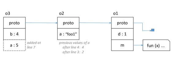
Figure 2: Runtime heap for Figure 1 at line 6.

JavaScript field accesses also present a challenge for AOTC. Figure 2 shows a runtime heap layout of the three objects allocated in Figure 1 (after line 6). In JavaScript, a field read x.f first checks x for field f, and continues up x’s prototype chain until f is found. If f is not found, the read evaluates to undefined. Field writes x.f = y are peculiar. If f exists in x, it is updated in place. If not, f is created in x, even if f is available up the prototype chain. This peculiarity is often a source of bugs. For our example, the write to this.a within the invocation v3.m(4) on line 7 creates a new slot in o3 (dashed box in Figure 2), rather than updating o2.a.

Besides being a source of bugs, this field write behavior prevents a compiler from optimizing field lookups. If the set of fields in every object is fixed at the time of allocation—a fixed object layout Choi et al. [2015b]—then the compiler can use a constant indirection table for field offsets. Fixed layout also establishes the availability of fields for reading / writing, obviating the need for runtime checks.

In summary, our type system must enforce the following properties:

• Type compatibility, e.g., integer and string values cannot be assigned to the same variable.

• Access safety of object fields: fields that are neither available locally nor in the prototype chain cannot be read; and fields that are not locally available cannot be written.

These properties promote good programming practices and make code more amenable to compilation. Note that detection of errors that require flow-sensitive reasoning, like null dereferences, is out of scope for our type system; extant systems like TAJS Jensen et al. [2009] can be applied to find such issues.

2.2 The Type System

Access safety. In our type system, the fields in an object type $O$ are maintained as two rows (maps from field names to types), $O^{\mathsf{r}}$ for readable fields and $O^{\mathsf{w}}$ for writeable fields. Readable fields are those present either locally or in the prototype chain, while writeable fields must be present locally (and hence must also be readable). Since o1 in Figure 1 only has local fields $d$ and $m$, we have $O_{1}^{\mathsf{r}}=O_{1}^{\mathsf{w}}=\langle d,m\rangle$. For o2, the readable fields $O_{2}^{\mathsf{r}}$ include local fields $\langle a\rangle$ and fields $\langle d,m\rangle$ inherited from o1, so we have $O_{2}^{\mathsf{r}}=\langle d,m,a\rangle$ and $O_{2}^{\mathsf{w}}=\langle a\rangle$. Similarly, $O_{3}^{\mathsf{r}}=\langle d,m,a,b\rangle$ and $O_{3}^{\mathsf{w}}=\langle b\rangle$. The type system rejects writes to read-only fields; e.g., v2.d = 2 would be rejected.

Detecting that the call v3.m(4) on line 7 violates access safety is less straightforward. To handle this case, the type system tracks two additional rows for certain object types: the fields that attached methods may read ($O^{\mathsf{mr}}$), and those that methods may write ($O^{\mathsf{mw}}$). The typing rules ensure that such method-accessed fields for an object type include the fields of the receiver types for all attached methods. Let $T_{m}$ be the receiver type for method m (LABEL:li:m-attach). Based on the uses of this within m, we have $T_{m}^{\mathsf{r}}=\langle d,a\rangle$ and $T_{m}^{\mathsf{w}}=\langle a\rangle$ (again, writeable fields must be readable). Since m is the only method attached to o1, we have $O_{1}^{\mathsf{mr}}=T_{m}^{\mathsf{r}}=\langle d,a\rangle$ and $O_{1}^{\mathsf{mw}}=T_{m}^{\mathsf{w}}=\langle a\rangle$. Since o2 and o3 inherit m and have no other methods, we also have $O_{3}^{\mathsf{mr}}=O_{2}^{\mathsf{mr}}=\langle d,a\rangle$ and $O_{3}^{\mathsf{mw}}=O_{2}^{\mathsf{mw}}=\langle a\rangle$.

With these types, we have $\mathtt{a}\in O_{3}^{\mathsf{mw}}$ and $\mathtt{a}\not\in O_{3}^{\mathsf{w}}$: i.e., a method of $O_{3}$ can write field field a, which is not locally present. Hence, the method call v3.m(4) is unsafe. The type system considers $O_{3}$ to be abstract, and method invocations on abstract types are rejected. (Types for which method invocations are safe are concrete.) Similarly, $O_{1}$ is also abstract. Note that rejecting abstract types completely is too restrictive: JavaScript code often has prototype objects that are abstract, with methods referring to fields declared only in inheritors.

The idea of tracking method-accessed fields follows the type system of Choi et al. Choi et al. [2015b, a], but they did not distinguish between $\mathsf{mr}$ and $\mathsf{mw}$, essentially placing all accessed fields in $\mathsf{mw}$. Their treatment would reject the safe call at LABEL:li:m-call-int, whereas with $\mathsf{mr}$, we are able to type it.

Subtyping. A type system for JavaScript must also support structural subtyping between object types to handle common idioms. But, a conflict arises between structural subtyping and tracking of method-accessed fields. Consider the following code:

⬇

1p = cond()

2 ? { m : fun() { this.f = 1 }, f: 2 } // o1

3 : { m : fun() { this.g = 2 }, g: 3 } // o2

4p.m();

Both o1 and o2 have concrete types, as they contain all fields accessed by their methods. Since m is the only common field between o1 and o2, by structural subtyping, m is the only field in the type of p. But what should the method-writeable fields of p be? A sound approach of taking the union of such fields from o1 and o2 yields $\langle f,g\rangle$. But, this makes the type of p abstract (neither $f$ nor $g$ is present in p), prohibiting the safe call of p.m().

To address this issue, we adopt ideas from previous work Choi et al. [2015b]; Palsberg and Zhao [2004] and distinguish prototypal types, suitable for prototype inheritance, from non-prototypal types, suitable for structural subtyping. Non-prototypal types elide method-accessed fields, thereby avoiding bad interactions with structural subtyping. For the example above, we can assign p a non-prototypal concrete type, thereby allowing the p.m() call. However, an expression {...} proto p would be disallowed: without method-accessed field information for p, inheritance cannot be soundly handled. For further details, see Section 3.3.

2.3 Inference Challenges

As noted in Section 1, we found that no extant type inference technique was suitable for our needs. The closest techniques are those that reason about prototype inheritance precisely, like type inference for Self Agesen et al. [1993] and the TAJS system for JavaScript Jensen et al. [2009]. Both of these systems work by tracking which values may flow to an operation (a “top-down” approach), and then ensuring the operation is legal for those values. They also gain significant scalability by only analyzing reachable code, as determined by the analysis itself. But, this approach cannot infer types or find type errors in unreachable code, e.g., a function under development that is not yet invoked. Consider this example:

⬇

1function f(x) {

2 var y = -x;

3 return x[1];

4}

5f(2);

Without the final call f(2), the previous techniques would not find the (obvious) type error within f. This limitation is unacceptable, as developers expect a compiler to report errors in all code.

An alternative inference approach is to compute types based on how variables/expressions are used (a “bottom-up” approach), and then check any incoming values against these types. Such an approach is standard in unification-style inference algorithms, combined with introduction of parametric polymorphism to generalize types as appropriate Damas and Milner [1982]. Unfortunately, since our type system has subtyping, we cannot apply such unification-based techniques, nor can we easily infer parametric polymorphism.

Instead, our inference takes a hybrid approach, tracking value flow in lower bounds of type variables and uses in upper bounds. Both bounds are sets of types, and the final ascribed type must be a subtype of all upper bound types and a supertype of all lower bound types. Upper bounds enable type inference and error discovery for uninvoked functions, e.g., discovery of the error within f above.

If upper bounds alone under-constrain a type, lower bounds provide a further constraint to inform ascription. For example, given the identity function id(x) { return x; }, since no operations are performed on x, upper bounds give no information on its type. However, if there is an invocation id("hi"), inference can use the lower bound information from "hi" to ascribe the type $\mathsf{string}\rightarrow\mathsf{string}$. Note that as in other systems typ ; flo , we could combine our inference with checking of user-written polymorphic types, e.g., if the user provided a type $T\rightarrow T$ ($T$ is a type variable) for id.

Once all upper and lower bounds are computed, an assignment needs to be made to each type variable. A natural choice is the greatest lower bound of the upper bounds, with a further check that the result is a supertype of all lower bound types. However, if upper and lower bounds are based solely on value flow and uses, type variables can be partially constrained, with $\emptyset$ as the upper bound (if there are no uses) or the lower bound (if no values flow in). In the first case, since our type system does not include a top type, it is not clear what assignment to make. This is usually not a concern in unification-based analyses, which flow information across assignments symmetrically, but it is an issue in subtyping-based analyses such as ours.

Particular care thus needs to be taken to soundly assign type variables whose upper bound is empty. A sound choice would be to simply fail in inference, but this would be too restrictive. We could compute an assignment based on the lower bound types, e.g., their least upper bound. But this scheme is unsound, as shown by the following example:

⬇

function f(x) {

var y = x; y = 2; return x.a+1;

}

Assume f is uninvoked. Using a graphical notation (edges reflect subtyping), the relevant constraints for this code are:

x has no incoming value flow, but it is used as an object with an integer $a$ field (shown as the $X^{\mathsf{r}}\longrightarrow\langle a:\mathsf{int}\rangle$ edge). For y, we see no uses, but the integer 2 flows into it (shown as the $Y^{\mathsf{r}}\longleftarrow\mathsf{int}$ edge). A technique based solely on value flow and uses would compute the upper bound of $X^{\mathsf{r}}$ as $\left\{\langle a:\mathsf{int}\rangle\right\}$, the lower bound of $Y^{\mathsf{r}}$ as $\left\{\mathsf{int}\right\}$, and the lower bound of $X^{\mathsf{r}}$ and upper bound of $Y^{\mathsf{r}}$ as $\emptyset$. But, ascribing types based on these bounds would be unsound: they do not capture the fact that if x is ascribed an object type, then y must also be an object, due to the assignment y = x.

Instead, our inference strengthens lower bounds based on upper bounds, and vice-versa. For the above case, bound strengthening yields the following constraints (edges due to strengthening are dashed):

Given the type $\langle a:\mathsf{int}\rangle$ in the upper bound of $X^{\mathsf{r}}$, we strengthen $X^{\mathsf{r}}$’s lower bound to $\bot_{\mathsf{row}}$ (a subtype of all rows), as we know that any type-correct value flowing into x must be an object. As $Y^{\mathsf{r}}$ is now reachable from $\bot_{\mathsf{row}}$, $\bot_{\mathsf{row}}$ is added to $Y^{\mathsf{r}}$’s lower bound. With this bound, the algorithm strengthens $Y^{\mathsf{r}}$’s upper bound to $\langle\ \rangle$, a supertype of all rows. Given these strengthened bounds, inference tries to ascribe an object type to y, and detects a type error with $\mathsf{int}$ in $Y^{\mathsf{r}}$’s lower bound, as desired. Apart from aiding in correctness, bound strengthening simplifies ascription, as any type variable can be ascribed the greatest-lower bound of its upper bound (details in Section 4.2).

3 Terms, Types, and Constraint Generation

This section details the terms and types for a core calculus based on that of Choi et al. Choi et al. [2015a], modelling a JavaScript fragment equipped with integers, objects, prototype inheritance, and methods. The type system includes structural subtyping, abstract types, and recursive types. As this paper focuses on inference, rather than presenting the typing relation here, we show the constraint generation rules for inference instead, which also capture the requirements for terms to be well-typed. Appendix B presents the full typing relation.

$$\begin{array}[]{l@{~~}r@{~~}c@{~~}l}\textbf{fields}\hfil~{}~{}&a~{}~{}&\in\hfil~{}~{}&\mathcal{A}\\ \textbf{expressions}\hfil~{}~{}&e~{}~{}&::=\hfil~{}~{}&n\mid\mathsf{let}~{}x=e_{1}~{}\mathsf{in}~{}e_{2}\mid x\mid x:=e_{1}\\ \lx@intercol\quad\mid\left\{\cdot\right\}\mid\left\{a_{1}:e_{1},\ldots,a_{n}:e_{n}\right\}~{}\textsf{proto}~{}e_{p}\mid\mathsf{null}\mid\mathsf{this}\hfil\lx@intercol\\ \lx@intercol\quad\mid e.a\mid e_{1}.a:=e_{2}\mid\mathsf{function}\left(x\right)\left\{e_{1}\right\}\mid e_{1}.a\left(e_{2}\right)\hfil\lx@intercol\\ \end{array}$$

Figure 3: Syntax of terms.

3.1 Terms

Figure 3 presents the syntax of the calculus. The metavariable $a$ ranges over a finite set of fields $\mathcal{A}$, which describe the fields of objects. Expressions $e$ include base terms $n$ (which we take to be integers), and variable declaration ($\mathsf{let}~{}x=e_{1}~{}\mathsf{in}~{}e_{2}$), use ($x$), and assignment ($x:=e$). An object is either the empty object $\left\{\cdot\right\}$ or a record of fields $\left\{a_{1}:e_{1},\ldots,a_{n}:e_{n}\right\}~{}\textsf{proto}~{}e_{p}$, where $e_{p}$ is the object’s prototype. We also have the $\mathsf{null}$ and the receiver, $\mathsf{this}$.

Field projection $e.a$ and assignment $e_{1}.a:=e_{2}$ take the expected form. The calculus includes first-class methods (declared with the $\mathsf{function}$ syntax, as in JavaScript), which must be invoked with a receiver argument. Our implementation also handles first-class functions, but they present no additional complications for inference beyond methods, so we omit them here for simplicity. Appendix B gives details.

3.2 Types

$$\begin{array}[]{l@{~~}r@{~~}c@{~~}l}\textbf{types}\hfil~{}~{}&\hbox to0.0pt{\hss$\tau,\sigma\in\mathcal{T}$}~{}~{}&::=\hfil~{}~{}&\mathsf{int}\mid\nu\mid\alpha\mid\\ \hfil~{}~{}&~{}~{}&\mid\hfil~{}~{}&\left[\nu\right]\tau_{1}\Rightarrow\tau_{2}\mid\left[\cdot\right]\tau_{1}\Rightarrow\tau_{2}\\ \textbf{rows}\hfil~{}~{}&r,w,mr,mw~{}~{}&::=\hfil~{}~{}&\langle a_{1}:\tau_{1},\ldots,a_{n}:\tau_{n}\rangle\\ \textbf{base types}\hfil~{}~{}&\rho~{}~{}&::=\hfil~{}~{}&\left\{r\mid w\right\}\\ \textbf{object types}\hfil~{}~{}&\nu~{}~{}&::=\hfil~{}~{}&\rho^{q}\mid\mu\alpha.\nu\\ \textbf{qualifiers}\hfil~{}~{}&q~{}~{}&::=\hfil~{}~{}&{\mathbf{P}\left(mr,mw\right)}\mid\mathbf{NC}\mid\mathbf{NA}\\ \end{array}$$

Figure 4: Syntax of types.

Figure 4 presents the syntax of types. Types $\tau$ include a base type (integers), objects ($\nu$), and two method types: unattached methods ($\left[\tau_{r}\right]\tau_{1}\Rightarrow\tau_{2}$), which retain the receiver type $\tau_{r}$, and attached methods ($\left[\cdot\right]\tau_{1}\Rightarrow\tau_{2}$), wherein the receiver type is elided and assumed to be the type of the object to which the method is attached. (If $e_{1}.a:=e_{2}$ assigns a new method to $e_{1}.a$, $e_{2}$ is typed as an unattached method. Choi et al Choi et al. [2015b] restricted $e_{2}$ to method literals, whereas our treatment is more general.)

Object types comprise a base type, $\rho$, and a qualifier, $q$. The base type is a pair of rows (finite maps from names to types), one for the readable fields $r$ and one for the writeable fields $w$. Well-formedness for object types (detailed in Section 3.3) requires that writeable fields are also readable. We choose to repeat the fields of $w$ into $r$ in this way because it enables a simpler mathematical treatment based on row subtyping. Object types also contain recursive object types $\mu\alpha.\nu$, where $\alpha$ is bound in $\nu$ and may appear in field types.

Object qualifiers $q$ describe the field accesses performed by the methods in the type, required for reasoning about access safety (see Section 2.2). A prototypal qualifier ${\mathbf{P}\left(mr,mw\right)}$ maintains the information explicitly with two rows, one for fields readable by methods of the type ($mr$), and another for method-writeable fields ($mw$). At a method call, the type system ensures that all method-readable fields are readable on the base object, and similarly for method-writeable fields. The $\mathbf{NC}$ and $\mathbf{NA}$ qualifiers are used to enable structural subtyping on object types, and are discussed further in Section 3.3.

3.3 Subtyping and Type Equivalence

S-Row $$\displaystyle{\hbox{\hskip 81.13489pt\vbox{\hbox{\hskip-81.13487pt\hbox{\hbox{$\displaystyle\displaystyle\forall a\in\mathsf{dom(}r^{\prime}\mathsf{)}.a\in\mathsf{dom(}r\mathsf{)}\wedge r[a]\equiv r^{\prime}[a]$}}}\vbox{}}}\over\hbox{\hskip 15.83716pt\vbox{\vbox{}\hbox{\hskip-15.83716pt\hbox{\hbox{$\displaystyle\displaystyle{r\ \mathsf{<:}\ r^{\prime}}$}}}}}} \displaystyle{\hbox{\hskip 83.75516pt\vbox{\hbox{\hskip-83.75514pt\hbox{\hbox{$\displaystyle\displaystyle r_{1}\ \mathsf{<:}\ r_{2}\quad w_{1}\ \mathsf{<:}\ w_{2}\quad k=\mathbf{NC}\vee k=\mathbf{NA}$}}}\vbox{}}}\over\hbox{\hskip 45.63152pt\vbox{\vbox{}\hbox{\hskip-45.6315pt\hbox{\hbox{$\displaystyle\displaystyle{\left\{r_{1}\mid w_{1}\right\}^{k}\ \mathsf{<:}\ \left\{r_{2}\mid w_{2}\right\}^{k}}$}}}}}} \displaystyle{\hbox{\hskip 89.30658pt\vbox{\hbox{\hskip-89.30656pt\hbox{\hbox{$\displaystyle\displaystyle r_{1}\equiv r_{2}\quad w_{1}\equiv w_{2}\quad mr_{1}\equiv mr_{2}\quad mw_{1}\equiv mw_{2}$}}}\vbox{}}}\over\hbox{\hskip 72.1377pt\vbox{\vbox{}\hbox{\hskip-72.13768pt\hbox{\hbox{$\displaystyle\displaystyle{\left\{r_{1}\mid w_{1}\right\}^{\mathbf{P}\left(mr_{1},mw_{1}\right)}\ \mathsf{<:}\ \left\{r_{2}\mid w_{2}\right\}^{\mathbf{P}\left(mr_{2},mw_{2}\right)}}$}}}}}} \displaystyle{\hbox{\hskip 46.55336pt\vbox{\hbox{\hskip-46.55334pt\hbox{\hbox{$\displaystyle\displaystyle r\ \mathsf{<:}\ mr\quad w\ \mathsf{<:}\ mw$}}}\vbox{}}}\over\hbox{\hskip 56.3276pt\vbox{\vbox{}\hbox{\hskip-56.32759pt\hbox{\hbox{$\displaystyle\displaystyle{\left\{r\mid w\right\}^{\mathbf{P}\left(mr,mw\right)}\ \mathsf{<:}\ \left\{r\mid w\right\}^{\mathbf{NC}}}$}}}}}} \displaystyle{\hbox{}\over\hbox{\hskip 55.2943pt\vbox{\vbox{}\hbox{\hskip-55.29428pt\hbox{\hbox{$\displaystyle\displaystyle{\left\{r\mid w\right\}^{\mathbf{P}\left(mr,mw\right)}\ \mathsf{<:}\ \left\{r\mid w\right\}^{\mathbf{NA}}}$}}}}}} \displaystyle{\hbox{}\over\hbox{\hskip 47.48424pt\vbox{\vbox{}\hbox{\hskip-47.48422pt\hbox{\hbox{$\displaystyle\displaystyle{\left\{r\mid w\right\}^{\mathbf{NC}}\ \mathsf{<:}\ \left\{r\mid w\right\}^{\mathbf{NA}}}$}}}}}} \displaystyle{\hbox{}\over\hbox{\hskip 46.52884pt\vbox{\vbox{}\hbox{\hskip-46.52882pt\hbox{\hbox{$\displaystyle\displaystyle{\left[\tau\right]\tau_{1}\Rightarrow\tau_{2}\ \mathsf{<:}\ \left[\cdot\right]\tau_{1}\Rightarrow\tau_{2}}$}}}}}} \displaystyle{\hbox{\hskip 39.89868pt\vbox{\hbox{\hskip-39.89867pt\hbox{\hbox{$\displaystyle\displaystyle\tau_{1}\ \mathsf{<:}\ \tau_{2}\quad\tau_{2}\ \mathsf{<:}\ \tau_{3}$}}}\vbox{}}}\over\hbox{\hskip 17.44934pt\vbox{\vbox{}\hbox{\hskip-17.44933pt\hbox{\hbox{$\displaystyle\displaystyle\tau_{1}\ \mathsf{<:}\ \tau_{3}$}}}}}} \displaystyle{\hbox{}\over\hbox{\hskip 14.64934pt\vbox{\vbox{}\hbox{\hskip-14.64932pt\hbox{\hbox{$\displaystyle\displaystyle\tau\ \mathsf{<:}\ \tau$}}}}}}$$       S-NonProto        S-Proto        S-ProtoConc        S-ProtoAbs        S-ConcAbs        S-Method        S-Trans        S-Refl 

WF-NonObject $$\displaystyle{\hbox{\hskip 89.74149pt\vbox{\hbox{\hskip-89.74149pt\hbox{\hbox{$\displaystyle\displaystyle\textrm{$\displaystyle\tau$ is not an object type or a type variable}$}}}\vbox{}}}\over\hbox{\hskip 12.74127pt\vbox{\vbox{}\hbox{\hskip-12.74127pt\hbox{\hbox{$\displaystyle\displaystyle\Delta\Vdash\tau$}}}}}} \displaystyle{\hbox{\hskip 70.6285pt\vbox{\hbox{\hskip-70.6285pt\hbox{\hbox{$\displaystyle\displaystyle r\ \mathsf{<:}\ w\quad\forall a\in\mathsf{dom(}r\mathsf{)}.\ \Delta\Vdash{r}[a]$}}}\vbox{}}}\over\hbox{\hskip 27.73099pt\vbox{\vbox{}\hbox{\hskip-27.73097pt\hbox{\hbox{$\displaystyle\displaystyle\Delta\Vdash\left\{r\mid w\right\}^{\mathbf{NC}}$}}}}}} \displaystyle{\hbox{\hskip 70.6285pt\vbox{\hbox{\hskip-70.6285pt\hbox{\hbox{$\displaystyle\displaystyle r\ \mathsf{<:}\ w\quad\forall a\in\mathsf{dom(}r\mathsf{)}.\ \Delta\Vdash{r}[a]$}}}\vbox{}}}\over\hbox{\hskip 27.80876pt\vbox{\vbox{}\hbox{\hskip-27.80875pt\hbox{\hbox{$\displaystyle\displaystyle\Delta\Vdash\left\{r\mid w\right\}^{\mathbf{NA}}$}}}}}} \displaystyle{\hbox{\hskip 180.58759pt\vbox{\hbox{\hskip-70.6285pt\hbox{\hbox{$\displaystyle\displaystyle r\ \mathsf{<:}\ w\quad\forall a\in\mathsf{dom(}r\mathsf{)}.\ \Delta\Vdash{r}[a]$}}}\vbox{\hbox{\hskip-180.58757pt\hbox{\hbox{$\displaystyle\displaystyle mr\ \mathsf{<:}\ mw\quad\forall a\in\mathsf{dom(}mr\mathsf{)}.\ \Delta\Vdash{mr}[a]$}\hskip 20.00003pt\hbox{\hbox{$\displaystyle\displaystyle\forall a\in\mathsf{dom(}mr\mathsf{)}\cap\mathsf{dom(}r\mathsf{)}.\ mr[a]\equiv r[a]$}}}}\vbox{}}}}\over\hbox{\hskip 36.65213pt\vbox{\vbox{}\hbox{\hskip-36.65211pt\hbox{\hbox{$\displaystyle\displaystyle\Delta\Vdash\left\{r\mid w\right\}^{\mathbf{P}\left(mr,mw\right)}$}}}}}} \displaystyle{\hbox{\hskip 18.44614pt\vbox{\hbox{\hskip-18.44612pt\hbox{\hbox{$\displaystyle\displaystyle\Delta,\alpha\Vdash\nu$}}}\vbox{}}}\over\hbox{\hskip 21.45888pt\vbox{\vbox{}\hbox{\hskip-21.45886pt\hbox{\hbox{$\displaystyle\displaystyle\Delta\Vdash\mu\alpha.\nu$}}}}}} \displaystyle{\hbox{}\over\hbox{\hskip 19.17473pt\vbox{\vbox{}\hbox{\hskip-19.17473pt\hbox{\hbox{$\displaystyle\displaystyle\Delta,\alpha\Vdash\alpha$}}}}}}$$       WF-NC        WF-NA        WF-P        WF-Rec        WF-Var 

Figure 5: Subtyping and object-type well-formedness.

Any realistic type system for JavaScript must support structural subtyping for object types. Figure 5 presents the subtyping rules for our type system. In the premises, we sometimes write $\tau_{1}\equiv\tau_{2}$ as a shorthand for $\tau_{1}\ \mathsf{<:}\ \tau_{2}\land\tau_{2}\ \mathsf{<:}\ \tau_{1}$, and similarly $r_{1}\equiv r_{2}$ as a shorthand for $r_{1}\ \mathsf{<:}\ r_{2}\land r_{2}\ \mathsf{<:}\ r_{1}$. The S-Row rule enables width subtyping on rows and row reordering, and the S-NonProto rule lifts those properties to nonprototypal objects (ignore the qualifier $k$ for the moment). Note from S-Row that overlapping field types must be equivalent, disallowing depth subtyping—such subtyping is known to be unsound with mutable fields Fisher and Mitchell [1995]; Abadi and Cardelli [1996]. Depth subtyping would be sound for read-only fields, but we disallow it to simplify inference.

As discussed in Section 2.2, there is no good way to preserve information about method-readable and method-writeable fields across use of structural subtyping. Hence, other than row reordering enabled by S-Row and S-Proto, there is no subtyping between distinct prototypal types, which are the ones that carry method-readable and method-writeable information. To employ structural subtyping, a prototypal type must first be converted to a non-prototypal $\mathbf{NC}$ or $\mathbf{NA}$ type (distinction to be discussed shortly), using the S-ProtoConc or S-ProtoAbs rules. After this conversion, structural subtyping is possible using S-NonProto. Since non-prototypal types have no specific information about which fields are accessed by methods, they cannot be used for prototype inheritance or method updates; see Section 3.5.

The type system also makes a distinction between concrete object types, on which method invocations are allowed, and abstract types, for which invocations are prohibited. For prototypal types, concreteness can be checked directly, by ensuring that all method-readable fields are readable on the object and similarly for method-writeable fields, i.e., $r\ \mathsf{<:}\ mr$ and $w\ \mathsf{<:}\ mw$ (the assumptions of the S-ProtoConc rule). For non-prototypal types, we employ separate qualifiers $\mathbf{NC}$ and $\mathbf{NA}$ to distinguish concrete from abstract. Rule S-ProtoConc only allows concrete prototypal types to be converted to an $\mathbf{NC}$ type, whereas rule S-ProtoAbs allows any prototypal type to be converted to an $\mathbf{NA}$ type. The type system only allows a method call if the receiver type can be converted to an $\mathbf{NC}$ type (see Section 3.5). The S-ConcAbs rule allows any $\mathbf{NC}$ type to be converted to the corresponding $\mathbf{NA}$ type, as this only removes the ability to invoke methods.

Revisiting the example in Figure 1, here are the types for objects $O_{1}$, $O_{2}$ and $O_{3}$.

$$O_{1} :\left\{\langle d:\mathsf{int},m:\left[\cdot\right]\mathsf{int}\Rightarrow\mathsf{void}\rangle\mid\langle d,m\rangle\right\}^{{\mathbf{P}\left(\langle d,a\rangle,\langle a\rangle\right)}}$$

$$O_{2} :\left\{\langle d:\mathsf{int},m:\left[\cdot\right]\mathsf{int}\Rightarrow\mathsf{void},a:\mathsf{int}\rangle\mid\langle a\rangle\right\}^{{\mathbf{P}\left(\langle d,a\rangle,\langle a\rangle\right)}}$$

$$O_{3} :\left\{\langle d:\mathsf{int},m:\left[\cdot\right]\mathsf{int}\Rightarrow\mathsf{void},a:\mathsf{int},b:\mathsf{int}\rangle\mid\langle b\rangle\right\}^{{\mathbf{P}\left(\langle d,a\rangle,\langle a\rangle\right)}}$$

(We omit writing the types of fields in rows duplicatively.) In view of the subtyping relation presented above, the conversion of the prototypal type of $O_{2}$ to a $\mathbf{NC}$ type is allowed (by S-ProtoConc), so a method call at line LABEL:li:m-call-int is allowed. By contrast, the conversion of the prototypal type of $O_{3}$ to a $\mathbf{NC}$ type is not allowed (because the condition $w\ \mathsf{<:}\ mw$ is not satisfied in S-ProtoConc), and so the method call at line 7 is disallowed. Figure 6 gives a graphical view of the associated type lattice, showing the order between prototypal, $\mathbf{NC}$ and $\mathbf{NA}$ types.

Figure 6: Lattice of object types

The $\mathbf{NA}$ qualifier aids in expressivity. Consider extending Figure 1 as follows:

⬇

8 var v4 = cond() ? /*@\label{li:v4-def}@*/

9 v3 :

10 { d : 2 } // o4

The type of $O_{4}$ is $\left\{\langle d:\mathsf{int}\rangle\mid\langle d\rangle\right\}^{{\mathbf{P}\left(\langle\ \rangle,\langle\ \rangle\right)}}$. To ascribe a type to v4, we need to find a common supertype of the types of $O_{3}$ and $O_{4}$. We cannot simply upcast $O_{3}$ to the type of $O_{4}$ because there is no subtyping on prototypal types; S-NonProto does not apply. We also cannot apply S-ProtoConc to $O_{3}$, as $O_{3}$ is not concrete. However, we can use S-ProtoAbs and S-NonProto, in that order, to upcast the type of $O_{3}$ to $\left\{\langle d:\mathsf{int}\rangle\mid\langle\ \rangle\right\}^{\mathbf{NA}}$ (see Figure 6). This type is also a supertype of the type of $O_{4}$, and therefore, a suitable type to be ascribed to v4. $\mathbf{NA}$ serves as a top element in the object type lattice, which also simplifies type ascription as we will illustrate in Section 4.2.

Rule S-Method introduces a limited form of method subtyping to allow an unattached method to be attached to an object, thereby losing its receiver type. This stripping of receiver types is important for object subtyping. In the subtyping example in Section 2.2, without attached methods, o1 and o2 would not have a common supertype with m present, as the receiver types for their m methods would differ; this would make p.m() a type error. We exclude any other form of method subtyping, as we have not encountered a need for it in practice. More general function/method subtyping poses additional challenges for inference, due to contravariance, but extant techniques could be adopted to handle these issues cois Pottier [1998, 2001]; we plan to do so when a practical need arises.

Subtyping is reflexive and transitive. Recursive types are equi-recursive and admit $\alpha$-equivalence, that is:

$${\mu\alpha.\nu} \ \mathsf{<:}\ \nu\left[\alpha\mapsto\mu\alpha.\nu\right]$$

$$\nu\left[\alpha\mapsto\mu\alpha.\nu\right] \ \mathsf{<:}\ {\mu\alpha.\nu}$$

$${\mu\alpha.\nu} \ \mathsf{<:}\ {\mu\beta.(\nu[\alpha\mapsto\beta])}$$

which directly implies:

$${\mu\alpha.\nu} \equiv\nu\left[\alpha\mapsto\mu\alpha.\nu\right]$$

$${\mu\alpha.\nu} \equiv{\mu\beta.(\nu[\alpha\mapsto\beta])}$$

Note that it is possible to expand a recursive type and then apply rule S-NonProto or S-Proto to achieve a form of width subtyping.

Figure 5 also shows the well-formedness for types, $\Delta\Vdash\tau$, in the context $\Delta$ representing a set of bound variables. All non-object non-variable types are well-formed (rule WF-NonObject). For object types, well-formedness requires that any writeable field is also readable, and that all field types are also well-formed (rules WF-NC and WF-NA). In prototypal types, well-formedness further requires that method-writeable fields are also method-readable, and that for any field $a$ that is both readable and method-readable, the $mr$ and $r$ rows agree on $a$’s type (rule WF-P). Finally, rules WF-Rec and WF-Var respectively introduce and eliminate type variables to enable well-formedness of recursive types.

3.4 Constraint Language

Here, we present the constraint language used to express our type inference problem. Constraints primarily operate over families of row variables, rather than directly constraining more complex source-level object types. Section 3.5 reduces inference for the source type system to this constraint language, and Section 4 gives an algorithm for solving such constraints.

$$\begin{array}[]{l@{~~}r@{~~}c@{~~}l}\textbf{type variables}\hfil~{}~{}&X,Y~{}~{}&\hfil~{}~{}&\textit{range over source types}\\ \textbf{variable sorts}\hfil~{}~{}&s~{}~{}&::=\hfil~{}~{}&\mathsf{r}\mid\mathsf{w}\mid\mathsf{mr}\mid\mathsf{mw}\mid\mathsf{all}\\ \textbf{row variables}\hfil~{}~{}&X^{s},Y^{s}~{}~{}&\hfil~{}~{}&\textit{range over row / non-object types}\\ \textbf{literals}\hfil~{}~{}&L~{}~{}&::=\hfil~{}~{}&\mathsf{int}\mid\bot_{\mathsf{row}}\mid\langle\ldots,a:X,\ldots\rangle\\ \hfil~{}~{}&~{}~{}&\hfil~{}~{}&\mid\left[X_{{\kern-0.5833pt}R}\right]X_{1}\Rightarrow X_{2}\\ \textbf{constraints}\hfil~{}~{}&C~{}~{}&::=\hfil~{}~{}&L\ \mathsf{<:}\ X^{s}\mid X^{s}\ \mathsf{<:}\ L\mid X^{s}\ \mathsf{<:}\ Y^{s}\\ \hfil~{}~{}&~{}~{}&\hfil~{}~{}&\mid C\land C\\ \hfil~{}~{}&~{}~{}&\hfil~{}~{}&\mid X^{s}\ \mathsf{<:}\ Y^{s}\backslash\left\{a_{1},\ldots,a_{n}\right\}\\ \hfil~{}~{}&~{}~{}&\hfil~{}~{}&\mid\mathsf{proto}(X)\mid\mathsf{concrete}\!\left(X\right)\\ \hfil~{}~{}&~{}~{}&\hfil~{}~{}&\mid\mathsf{strip}(X)\\ \hfil~{}~{}&~{}~{}&\hfil~{}~{}&\mid\mathsf{attach}(X_{b},X_{f},X_{v})\\ \textbf{acceptance criteria}\hfil~{}~{}&A~{}~{}&::=\hfil~{}~{}&\mathsf{notmethod}(X)\mid\mathsf{notproto}(X)\end{array}$$

$$\begin{array}[]{rl}\textbf{well-formedness}&X^{\mathsf{all}}\ \mathsf{<:}\ X^{\mathsf{r}}\ \mathsf{<:}\ X^{\mathsf{w}}\\ &\wedge\ X^{\mathsf{all}}\ \mathsf{<:}\ X^{\mathsf{mr}}\ \mathsf{<:}\ X^{\mathsf{mw}}\end{array}$$

Figure 7: Constraint language. We give the language syntax above the line, and well-formedness constraints below.

Figure 7 defines the constraint language syntax. The language distinguishes type variables, which represent source-level types, and row variables, which represent the various components of a source-level object type. Each type variable $X$ has five corresponding row variables: $X^{\mathsf{r}}$, $X^{\mathsf{w}}$, $X^{\mathsf{mr}}$, $X^{\mathsf{mw}}$, and $X^{\mathsf{all}}$. The first four correspond directly to the $r$, $w$, $mr$, and $mw$ rows from an object type. To enforce the condition $\Vdash\left\{r\mid w\right\}^{q}$ (Figure 5) on all types, we impose the well-formedness conditions in Figure 7 on all $X$. The last variable, $X^{\mathsf{all}}$, is used to ensure that types of fields in both $r$ and $mr$ are equivalent; if ascription fails for $X^{\mathsf{all}}$, there must be some inconsistency between $X^{\mathsf{r}}$ and $X^{\mathsf{mr}}$.

Type literals include $\mathsf{int}$, unattached methods, and rows. The $\bot_{\mathsf{row}}$ type ensures a complete row subtyping lattice and is used in type propagation (see Section 4.1). To handle non-object types, row variables are “overloaded” and can be assigned non-object types as well. Our constraints ensure that if any row variable for $X$ is assigned a non-row type $\tau$, then all row variables for $X$ will be assigned $\tau$, and hence $X$ should map to $\tau$ in the final ascription.

The first three constraint types introduced in Figure 7 express subtyping over literals and row variables. We write $X^{s}\equiv L$ as a shorthand for $L\ \mathsf{<:}\ X^{s}\land X^{s}\ \mathsf{<:}\ L$ and $X^{s}\equiv Y^{t}$ as a shorthand for $X^{s}\ \mathsf{<:}\ Y^{t}\land Y^{t}\ \mathsf{<:}\ X^{s}$. Constraints can be composed together using the $\land$ operator. A constraint $X^{s}\ \mathsf{<:}\ Y^{s}\backslash\left\{a_{1},\ldots,a_{n}\right\}$ means that $X^{s}$ must be a subtype of the type obtained by removing the fields $a_{1},\ldots,a_{n}$ from $Y^{s}$. Such constraints are needed for handling prototype inheritance, discussed further in Section 3.5.

The $\mathsf{proto}(X)$ and $\mathsf{concrete}\!\left(X\right)$ constraints enable inference of object type qualifiers. Constraint $\mathsf{proto}(X)$ means the ascribed type for $X$ must be prototypal, while $\mathsf{concrete}\!\left(X\right)$ means the type for $X$ must be a subtype of an $\mathbf{NC}$ type. The $\mathsf{strip}(X)$ constraint ensures $X$ is assigned an attached method type, with no receiver type. Conversion of unattached method types to attached occurs during ascription (Section 4.2), so the constraint syntax only includes unattached method types.

The constraint $\mathsf{attach}(X_{b},X_{f},X_{v})$ in Figure 7 handles method attachment to objects. For a field assignment $e_{1}.a:=e_{2}$, $X_{b}$, $X_{f}$, and $X_{v}$ respectively represent the type of $e_{1}$, the type of $a$ in $e_{1}$’s (object) type, and the type of $e_{2}$. Intuitively, this constraint ensures the following condition:

$$(X_{v}^{\mathsf{r}}\ \mathsf{<:}\ \left[X_{{\kern-0.5833pt}R}\right]\_\Rightarrow\_) \implies(\mathsf{proto}(X_{b})\ \wedge$$

$$X_{b}^{\mathsf{mr}}\ \mathsf{<:}\ X_{{\kern-0.5833pt}R}^{\mathsf{r}} \wedge X_{b}^{\mathsf{mw}}\ \mathsf{<:}\ X_{{\kern-0.5833pt}R}^{\mathsf{w}}\wedge\mathsf{strip}(X_{f}))$$

That is, when $X_{v}$ is an unattached method type with receiver $X_{{\kern-0.5833pt}R}$, then $X_{b}$ is prototypal, its method-readable and method-writeable fields must respectively include the readable and writeable fields of $X_{{\kern-0.5833pt}R}$, and $X_{f}$ is an attached method type. Note that $\mathsf{attach}(X_{b},X_{f},X_{v})$ is not a macro for the above condition, as we do not directly support an implication operator in the constraint language. Instead, the condition is enforced directly during constraint propagation (Figure 10, Rule (xii)).

The acceptance criteria in Figure 7 are additional conditions on solutions that need only be checked after the constraints have been solved. The two possible criteria are checking that a variable is not assigned a method type, $\mathsf{notmethod}(X)$, and ensuring a variable is not assigned a prototypal type, $\mathsf{notproto}(X)$.

3.5 Constraint Generation

Constraint generation takes the form of a judgement

$$X_{{\kern-0.5833pt}R},\Gamma\vdash e:X\mid C,$$

to be read as: in a context with receiver type $X_{{\kern-0.5833pt}R}$ and inference environment $\Gamma$, expression $e$ has type $X$ such that constraints in $C$ are satisfied. Figure 8 presents rules for constraint generation; see Section 4.1 for an example.

$$\framebox{$X_{{\kern-0.5833pt}R},\Gamma\vdash e:X\mid C$}\quad\raise 10.99165pt\hbox{\hbox{$\hbox{\small\small{C-Int}}\;$}${\hbox{$\displaystyle\displaystyle{\hbox{\hskip 16.65804pt\vbox{\hbox{\hskip-16.65802pt\hbox{\hbox{$\displaystyle\displaystyle\mathsf{fresh}~{}X$}}}\vbox{}}}\over\hbox{\hskip 48.39113pt\vbox{\vbox{}\hbox{\hskip-48.39111pt\hbox{\hbox{$\displaystyle\displaystyle X_{{\kern-0.5833pt}R},\Gamma\vdash n:X\mid X^{\mathsf{r}}\equiv\mathsf{int}$}}}}}}$}}\hbox{}$ }\penalty 50\hskip 20.00003pt plus 0.5fil minus 5.0pt\raise 10.72221pt\hbox{\hbox{$\hbox{\small\small{C-Var}}\;$}${\hbox{$\displaystyle\displaystyle{\hbox{\hskip 21.07288pt\vbox{\hbox{\hskip-21.07286pt\hbox{\hbox{$\displaystyle\displaystyle\Gamma(x)=X$}}}\vbox{}}}\over\hbox{\hskip 35.25508pt\vbox{\vbox{}\hbox{\hskip-35.25507pt\hbox{\hbox{$\displaystyle\displaystyle X_{{\kern-0.5833pt}R},\Gamma\vdash x:X\mid\emptyset$}}}}}}$}}\hbox{}$ }\penalty 50\hskip 20.00003pt plus 0.5fil minus 5.0pt\raise 10.72221pt\hbox{\hbox{$\hbox{\small\small{C-This}}\;$}${\hbox{$\displaystyle\displaystyle{\hbox{}\over\hbox{\hskip 48.73965pt\vbox{\vbox{}\hbox{\hskip-48.73964pt\hbox{\hbox{\hbox{$\displaystyle\displaystyle X_{{\kern-0.5833pt}R},\Gamma\vdash\mathsf{this}:X_{{\kern-0.5833pt}R}\mid\emptyset$}}\hskip 20.00003pt\hbox{$\displaystyle\displaystyle$}}}}}}$}}\hbox{}$ }\penalty 50\hskip 20.00003pt plus 0.5fil minus 5.0pt\raise 10.99165pt\hbox{\hbox{$\hbox{\small\small{C-VarDecl}}\;$}${\hbox{$\displaystyle\displaystyle{\hbox{\hskip 138.88007pt\vbox{\hbox{\hskip-138.88007pt\hbox{\hbox{$\displaystyle\displaystyle X_{{\kern-0.5833pt}R},\Gamma\left[x\mapsto X_{1}\right]\vdash e_{1}:Y_{1}\mid C_{1}$}\hskip 20.00003pt\hbox{\hbox{$\displaystyle\displaystyle\mathsf{fresh}~{}X_{1}$}\hskip 20.00003pt\hbox{\hbox{$\displaystyle\displaystyle X_{{\kern-0.5833pt}R},\Gamma\left[x\mapsto X_{1}\right]\vdash e_{2}:X\mid C_{2}$}}}}}\vbox{}}}\over\hbox{\hskip 126.06595pt\vbox{\vbox{}\hbox{\hskip-126.06595pt\hbox{\hbox{$\displaystyle\displaystyle X_{{\kern-0.5833pt}R},\Gamma\vdash\mathsf{let}~{}x=e_{1}~{}\mathsf{in}~{}e_{2}:X\mid C_{1}\wedge C_{2}\wedge Y_{1}^{\mathsf{r}}\ \mathsf{<:}\ X_{1}^{\mathsf{r}}\wedge Y_{1}^{\mathsf{w}}\ \mathsf{<:}\ X_{1}^{\mathsf{w}}$}}}}}}$}}\hbox{}$ }\penalty 50\hskip 20.00003pt plus 0.5fil minus 5.0pt\raise 10.99165pt\hbox{\hbox{$\hbox{\small\small{C-VarUpd}}\;$}${\hbox{$\displaystyle\displaystyle{\hbox{\hskip 68.37413pt\vbox{\hbox{\hskip-68.37413pt\hbox{\hbox{$\displaystyle\displaystyle x:X_{1}\in\Gamma$}\hskip 20.00003pt\hbox{\hbox{$\displaystyle\displaystyle X_{{\kern-0.5833pt}R},\Gamma\vdash e_{1}:X\mid C_{1}$}}}}\vbox{}}}\over\hbox{\hskip 101.98329pt\vbox{\vbox{}\hbox{\hskip-101.98328pt\hbox{\hbox{$\displaystyle\displaystyle X_{{\kern-0.5833pt}R},\Gamma\vdash x:=e_{1}:X\mid C_{1}\wedge X^{\mathsf{r}}\ \mathsf{<:}\ X_{1}^{\mathsf{r}}\wedge X^{\mathsf{w}}\ \mathsf{<:}\ X_{1}^{\mathsf{w}}$}}}}}}$}}\hbox{}$ }\penalty 50\hskip 20.00003pt plus 0.5fil minus 5.0pt\raise 11.26942pt\hbox{\hbox{$\hbox{\small\small{C-Null}}\;$}${\hbox{$\displaystyle\displaystyle{\hbox{\hskip 16.65804pt\vbox{\hbox{\hskip-16.65802pt\hbox{\hbox{$\displaystyle\displaystyle\mathsf{fresh}~{}X$}}}\vbox{}}}\over\hbox{\hskip 58.53783pt\vbox{\vbox{}\hbox{\hskip-58.53781pt\hbox{\hbox{$\displaystyle\displaystyle X_{{\kern-0.5833pt}R},\Gamma\vdash\mathsf{null}:X\mid X^{\mathsf{w}}\ \mathsf{<:}\ \langle\ \rangle$}}}}}}$}}\hbox{}$ }\penalty 50\hskip 20.00003pt plus 0.5fil minus 5.0pt\raise 17.26942pt\hbox{\hbox{$\hbox{\small\small{C-MethDecl}}\;$}${\hbox{$\displaystyle\displaystyle{\hbox{\hskip 115.82054pt\vbox{\hbox{\hskip-115.82054pt\hbox{\hbox{$\displaystyle\displaystyle\mathsf{fresh}~{}Y_{{\kern-0.5833pt}R},Y_{1},X\quad\mathsf{has\_this(}e\mathsf{)}\quad Y_{{\kern-0.5833pt}R},\Gamma\left[x\mapsto Y_{1}\right]\vdash e:Y_{2}\mid C$}}}\vbox{}}}\over\hbox{\hskip 200.84215pt\vbox{\vbox{}\hbox{\hskip-200.84215pt\hbox{\hbox{$\displaystyle\displaystyle X_{{\kern-0.5833pt}R},\Gamma\vdash\mathsf{function}\left(x\right)\left\{e\right\}:X\mid C\wedge Y_{{\kern-0.5833pt}R}^{\mathsf{w}}\ \mathsf{<:}\ \langle\ \rangle\wedge\mathsf{concrete}\!\left(Y_{{\kern-0.5833pt}R}\right)\wedge\mathsf{notproto}(Y_{{\kern-0.5833pt}R})\wedge X^{\mathsf{r}}\equiv(\left[Y_{{\kern-0.5833pt}R}\right]Y_{1}\Rightarrow Y_{2})$}}}}}}$}}\hbox{}$ }\penalty 50\hskip 20.00003pt plus 0.5fil minus 5.0pt\raise 23.26942pt\hbox{\hbox{$\hbox{\small\small{C-MethApp}}\;$}${\hbox{$\displaystyle\displaystyle{\hbox{\hskip 138.69104pt\vbox{\hbox{\hskip-138.69104pt\hbox{\hbox{$\displaystyle\displaystyle\mathsf{fresh}~{}X_{{\kern-0.5833pt}M},Y_{{\kern-0.5833pt}R},X_{3},X$}\hskip 20.00003pt\hbox{\hbox{$\displaystyle\displaystyle X_{{\kern-0.5833pt}R},\Gamma\vdash e_{1}:X_{1}\mid C_{1}\qquad X_{{\kern-0.5833pt}R},\Gamma\vdash e_{2}:X_{2}\mid C_{2}$}}}}\vbox{}}}\over\hbox{\hskip 359.92102pt\vbox{\vbox{}\hbox{\hskip-359.921pt\hbox{\hbox{$\displaystyle\displaystyle\begin{array}[]{l@{~}c@{~}l}X_{{\kern-0.5833pt}R},\Gamma\vdash e_{1}.a\left(e_{2}\right):X\mid\hfil~{}&\hfil~{}&C_{1}\wedge C_{2}\wedge X_{1}^{\mathsf{r}}\ \mathsf{<:}\ \langle a:X_{{\kern-0.5833pt}M}\rangle\wedge X_{{\kern-0.5833pt}M}^{\mathsf{r}}\equiv(\left[Y_{{\kern-0.5833pt}R}\right]X_{3}\Rightarrow X)\wedge\mathsf{strip}(X_{{\kern-0.5833pt}M})\wedge\mathsf{concrete}\!\left(X_{1}\right)\@arraycr&\wedge&\mathsf{concrete}\!\left(Y_{{\kern-0.5833pt}R}\right)\wedge Y_{{\kern-0.5833pt}R}^{\mathsf{w}}\ \mathsf{<:}\ \langle\ \rangle\wedge\mathsf{notproto}(Y_{{\kern-0.5833pt}R})\wedge X_{2}^{\mathsf{r}}\ \mathsf{<:}\ X_{3}^{\mathsf{r}}\wedge X_{2}^{\mathsf{w}}\ \mathsf{<:}\ X_{3}^{\mathsf{w}}\end{array}$}}}}}}$}}\hbox{}$ }\penalty 50\hskip 20.00003pt plus 0.5fil minus 5.0pt\raise 11.26942pt\hbox{\hbox{$\hbox{\small\small{C-ObjEmp}}\;$}${\hbox{$\displaystyle\displaystyle{\hbox{}\over\hbox{\hskip 96.6534pt\vbox{\vbox{}\hbox{\hskip-96.65338pt\hbox{\hbox{$\displaystyle\displaystyle X_{{\kern-0.5833pt}R},\Gamma\vdash\left\{\cdot\right\}:X\mid\mathsf{proto}(X)\wedge X^{\mathsf{r}}\equiv\langle\ \rangle\wedge X^{\mathsf{mr}}\equiv\langle\ \rangle$}}}}}}$}}\hbox{}$ }\quad\raise 11.26942pt\hbox{\hbox{$\hbox{\small\small{C-Attr}}\;$}${\hbox{$\displaystyle\displaystyle{\hbox{\hskip 58.10376pt\vbox{\hbox{\hskip-58.10376pt\hbox{\hbox{$\displaystyle\displaystyle\mathsf{fresh}~{}X\quad X_{{\kern-0.5833pt}R},\Gamma\vdash e:X_{1}\mid C$}}}\vbox{}}}\over\hbox{\hskip 113.53017pt\vbox{\vbox{}\hbox{\hskip-113.53017pt\hbox{\hbox{$\displaystyle\displaystyle X_{{\kern-0.5833pt}R},\Gamma\vdash e.a:X\mid C\wedge X_{1}^{\mathsf{r}}\ \mathsf{<:}\ \langle a:X\rangle\wedge\mathsf{notmethod}(X)$}}}}}}$}}\hbox{}$ }\penalty 50\hskip 20.00003pt plus 0.5fil minus 5.0pt\raise 17.53609pt\hbox{\hbox{$\hbox{\small\small{C-AttrUpd}}\;$}${\hbox{$\displaystyle\displaystyle{\hbox{\hskip 103.89223pt\vbox{\hbox{\hskip-103.89221pt\hbox{\hbox{$\displaystyle\displaystyle\mathsf{fresh}~{}X_{f}\quad X_{{\kern-0.5833pt}R},\Gamma\vdash e_{1}:X_{b}\mid C_{1}\quad X_{{\kern-0.5833pt}R},\Gamma\vdash e:X_{v}\mid C_{2}$}}}\vbox{}}}\over\hbox{\hskip 198.8874pt\vbox{\vbox{}\hbox{\hskip-198.88739pt\hbox{\hbox{$\displaystyle\displaystyle X_{{\kern-0.5833pt}R},\Gamma\vdash e_{1}.a:=e:X_{v}\mid C_{1}\wedge C_{2}\wedge X_{b}^{\mathsf{w}}\ \mathsf{<:}\ \langle a:X_{f}\rangle\wedge X_{v}^{\mathsf{r}}\ \mathsf{<:}\ X_{f}^{\mathsf{r}}\wedge X_{v}^{\mathsf{w}}\ \mathsf{<:}\ X_{f}^{\mathsf{w}}\wedge\mathsf{attach}(X_{b},X_{f},X_{v})$}}}}}}$}}\hbox{}$ }\penalty 50\hskip 20.00003pt plus 0.5fil minus 5.0pt\raise 29.26942pt\hbox{\hbox{$\hbox{\small\small{C-ObjLit}}\;$}${\hbox{$\displaystyle\displaystyle{\hbox{\hskip 185.4154pt\vbox{\hbox{\hskip-185.4154pt\hbox{\hbox{$\displaystyle\displaystyle\mathsf{fresh}~{}X\qquad\forall i\in 1..n.~{}\mathsf{fresh}~{}X_{i}\qquad\forall i\in 1..n.~{}X_{{\kern-0.5833pt}R},\Gamma\vdash e_{i}:Y_{i}\mid C_{i}\quad X_{{\kern-0.5833pt}R},\Gamma\vdash e_{p}:X_{p}\mid C_{p}$}}}\vbox{}}}\over\hbox{\hskip 451.10442pt\vbox{\vbox{}\hbox{\hskip-451.1044pt\hbox{\hbox{$\displaystyle\displaystyle\begin{array}[]{l@{~}c@{~}l}X_{{\kern-0.5833pt}R},\Gamma\vdash\left\{a_{1}:e_{1},\ldots,a_{n}:e_{n}\right\}~{}\textsf{proto}~{}e_{p}:X\mid\hfil~{}&\hfil~{}&C_{p}\wedge\bigwedge_{i}(C_{i}\wedge Y_{i}^{\mathsf{r}}\ \mathsf{<:}\ X_{i}^{\mathsf{r}}\wedge Y_{i}^{\mathsf{w}}\ \mathsf{<:}\ X_{i}^{\mathsf{w}}\wedge\mathsf{attach}(X,X_{i},Y_{i}))\@arraycr&\wedge&X^{\mathsf{w}}\equiv\langle a_{1}:X_{1},\ldots,a_{n}:X_{n}\rangle\wedge X^{\mathsf{r}}\ \mathsf{<:}\ X_{p}^{\mathsf{r}}\wedge X_{p}^{\mathsf{r}}\ \mathsf{<:}\ X^{\mathsf{r}}\backslash\left\{a_{1},\ldots,a_{n}\right\}\@arraycr&\wedge&\mathsf{proto}(X)\wedge\mathsf{proto}(X_{p})\wedge X^{\mathsf{mr}}\ \mathsf{<:}\ X_{p}^{\mathsf{mr}}\wedge X^{\mathsf{mw}}\ \mathsf{<:}\ X_{p}^{\mathsf{mw}}\end{array}$}}}}}}$}}\hbox{}$ }$$

Figure 8: Constraint generation.

Rules C-Int and C-Var generate straightforward constraints. The constraints for C-ObjEmp ensure the empty object is assigned type $\left\{\cdot\mid\cdot\right\}^{{\mathbf{P}\left(\cdot,\cdot\right)}}$. The rule C-This is the only rule directly using the carrier’s type $X_{{\kern-0.5833pt}R}$. The constraint $X^{\mathsf{w}}\ \mathsf{<:}\ \langle\ \rangle$ in rule C-Null ensures that $X$ is assigned an object type. (Recall that $X^{\mathsf{r}}\ \mathsf{<:}\ X^{\mathsf{w}}$.)

The rule for variable declaration C-VarDecl passes on the constraints generated by its subexpressions ($C_{1},C_{2}$), with additional constraints $Y_{1}^{\mathsf{r}}\ \mathsf{<:}\ X_{1}^{\mathsf{r}}\wedge Y_{1}^{\mathsf{w}}\ \mathsf{<:}\ X_{1}^{\mathsf{w}}$, which are sufficient to ensure that the type $Y_{1}$ of the expression $e_{1}$ is a subtype of the fresh inference variable $X_{1}$ ascribed to $x$ in the environment (no constraint on $Y_{1}^{\mathsf{mr}}$, $X_{1}^{\mathsf{mr}}$, $Y_{1}^{\mathsf{mw}}$ or $X_{1}^{\mathsf{mw}}$ is needed). Constraining both the $r$ and $w$ rows is consistent with the S-NonProto subtyping rule (Figure 5). We put $x$ in the initialization scope of $e_{1}$ in order to allow for the definition of recursive functions.

The C-MethDecl rule constrains the type of the body $e$ using fresh variables $Y_{1}$ and $Y_{{\kern-0.5833pt}R}$ for the parameter and receiver types. $Y_{{\kern-0.5833pt}R}$ is constrained to be non-prototypal and concrete, as in any legal method invocation, the receiver type must be a subtype of an $\mathbf{NC}$ type. (Recall that prototypal types, if they are concrete, can be safely cast to $\mathbf{NC}$.) The rule for method application C-MethApp ensures that the type $X_{1}$ of $e_{1}$ is concrete, and that its field $a$ has a method type $X_{{\kern-0.5833pt}M}$ with appropriate argument type $X_{3}$ and return type $X$. The $\mathsf{strip}(X_{{\kern-0.5833pt}M})$ constraint ensures $X_{{\kern-0.5833pt}M}$ is an attached method type. Note that a relation between $X_{1}$ and $Y_{{\kern-0.5833pt}R}$ is ensured by an $\mathsf{attach}$ constraint when method $a$ is attached to object $e_{1}$, following C-AttrUpd or C-ObjLit.

The last three rules deal more directly with objects. Constraint generation for attribute use C-Attr applies to non-methods (for methods, C-MethApp is used instead); the rule generates constraints requiring that $e$ has an object type $X_{1}$ with a readable field $a$, such that $a$ does not have a method type (preventing detaching of methods). The attribute update rule C-AttrUpd constrains $a$ to be a writable field of $e_{1}$ ($X_{b}^{\mathsf{w}}\ \mathsf{<:}\ \langle a:X_{f}\rangle$), and ensures that $X_{f}$ is a supertype of $e_{2}$’s type $X_{v}$. Finally, it uses the $\mathsf{attach}$ constraint to handle a possible method update.

Finally, the rule C-ObjLit imposes constraints governing object literals with prototype inheritance. Its constraints dwarf those of other rules, as object literals encompass potential method attachment for each field (captured by $\mathsf{attach}(X_{l},X_{i},Y_{i})$) in addition to prototype inheritance. For the literal type $X$, the constraints ensure that the writeable fields $X^{\mathsf{w}}$ are precisely those declared in the literal. The readable fields must include those inherited from the prototype ($X^{\mathsf{r}}\ \mathsf{<:}\ X_{p}^{\mathsf{r}}$); note that $X^{\mathsf{r}}\ \mathsf{<:}\ X^{\mathsf{w}}$ is imposed by well-formedness. Furthermore, the constraint $X_{p}^{\mathsf{r}}\ \mathsf{<:}\ X^{\mathsf{r}}\backslash\left\{a_{1},\ldots,a_{n}\right\}$ ensures that additional readable fields do not appear “out of thin air,” by requiring that any fields in $X^{\mathsf{r}}$ apart from the locally-present $a_{1},\ldots,a_{n}$ be present in the prototype. Finally, we ensure both $X$ and $X_{p}$ are prototypal, and that any method-accessed fields from $X_{p}$ are also present in $X$.

Figure 9: Selected constraints for the example of Figure 1.

Example Figure 9 shows a graph representation of some constraints for o1, o2, and v1 from lines 1–3 of Figure 1. Nodes represent row variables and type literals, with variable names matching the corresponding program entities ($Y_{{\kern-0.5833pt}R}$ corresponds to this on line LABEL:li:m-attach). Each edge $X^{s}\rightarrow Y^{t}$ represents a constraint $X^{s}\ \mathsf{<:}\ Y^{t}$. Black solid edges represent well-formedness constraints (Figure 7), while blue solid edges represent constraints generated from the code (Figure 8). Dashed or dotted edges are added during constraint solving, and will be discussed in Section 4.1.

We first discuss constraints for the body of the method declared on line LABEL:li:m-attach. For the field read this.d, the C-Attr rule generates $Y_{{\kern-0.5833pt}R}^{\mathsf{r}}\rightarrow\langle d:D\rangle$. Similarly, the C-AttrUpd rule generates $Y_{{\kern-0.5833pt}R}^{\mathsf{w}}\rightarrow\langle a:A\rangle$ for the write to this.a.

For the containing object literal o1, the C-ObjLit rule creates row variables for type $O_{1}$ and edges $O_{1}^{\mathsf{w}}\leftrightarrow\langle d:\mathsf{int},m:M\rangle$ (due to type equality). It also generates a constraint $\mathsf{attach}(O_{1},M,F)$ (not shown in Figure 9) to handle method attachment to field $m$ ($F$ is the type of the line LABEL:li:m-attach function); we shall return to this constraint in Section 4.1. The assignment to v1 yields the $V_{1}$ row variables and the $O_{1}^{\mathsf{r}}\rightarrow V_{1}^{\mathsf{r}}$ and $O_{1}^{\mathsf{w}}\rightarrow V_{1}^{\mathsf{w}}$ edges via C-VarDecl.

For o2 on line 3, C-ObjLit yields the $O_{2}^{\mathsf{w}}\leftrightarrow\langle a:\mathsf{int}\rangle$ edges for the declared a field. The use of v1 as a prototype yields the constraints $O_{2}^{\mathsf{r}}\rightarrow V_{1}^{\mathsf{r}}$, $O_{2}^{\mathsf{mr}}\rightarrow V_{1}^{\mathsf{mr}}$, and $O_{2}^{\mathsf{mw}}\rightarrow V_{1}^{\mathsf{mw}}$, capturing inheritance. We also have $V_{1}^{\mathsf{r}}\xrightarrow{\backslash\left\{a\right\}}O_{2}^{\mathsf{r}}$ to prevent "out of thin air" readable fields on $O_{2}$. Finally, we generate $\mathsf{proto}(V_{1})$ (not shown) to ensure $V_{1}$ gets a prototypal type.

4 Constraint Solving

Constraint solving proceeds in two phases. First, type propagation computes lower and upper bounds for every row variable, extending techniques from previous work Rastogi et al. [2012]; cois Pottier [1998]. Then, type ascription checks for type errors, and, if none are found, computes a satisfying assignment for the type variables.

4.1 Type Propagation

1. $\mathcal{C}\subseteq\mathcal{C^{\prime}}$;

Well-formedness

1. $X^{\mathsf{all}}\ \mathsf{<:}\ X^{\mathsf{r}}\ \mathsf{<:}\ X^{\mathsf{w}}\ \in\mathcal{C}^{\prime}$ and $X^{\mathsf{all}}\ \mathsf{<:}\ X^{\mathsf{mr}}\ \mathsf{<:}\ X^{\mathsf{mw}}\ \in\mathcal{C}^{\prime}$;

Subtyping

1. if $X^{s}\ \mathsf{<:}\ L\ \in\mathcal{C}^{\prime}$, then $L\in\left\lceil{X^{s}}\right\rceil$;

2. if $L\ \mathsf{<:}\ X^{s}\ \in\mathcal{C}^{\prime}$, then $L\in\left\lfloor{X^{s}}\right\rfloor$;

3. if $X^{s}\ \mathsf{<:}\ Y^{t}\ \in\mathcal{C}^{\prime}$, then $\left\lfloor{X^{s}}\right\rfloor\subseteq\left\lfloor{Y^{t}}\right\rfloor$ and $\left\lceil{Y^{t}}\right\rceil\subseteq\left\lceil{X^{s}}\right\rceil$;

4. if $X^{s}\ \mathsf{<:}\ Y^{t}\backslash\left\{a_{1},\ldots,a_{n}\right\}\ \in\mathcal{C}^{\prime}$, then for any $\langle F\rangle\in\left\lceil{Y^{t}}\right\rceil$, add $\langle F\backslash\left\{a_{1},\ldots,a_{n}\right\}\rangle$ to $\left\lceil{X^{s}}\right\rceil$;

Bound strengthening

1. if $L\in\left\lfloor{X^{s}}\right\rfloor$, then $\mathsf{top}(L)\in\left\lceil{X^{s}}\right\rceil$;

2. if $L\in\left\lceil{X^{s}}\right\rceil$, then $\mathsf{bot}(L)\in\left\lfloor{X^{s}}\right\rfloor$;

Prototypalness and concreteness

1. if $\mathsf{proto}(Y)\ \in\mathcal{C}^{\prime}$, $X^{\mathsf{r}}\ \mathsf{<:}\ Y^{\mathsf{r}}\ \in\mathcal{C}^{\prime}$ and $X^{\mathsf{w}}\ \mathsf{<:}\ Y^{\mathsf{w}}\ \in\mathcal{C}^{\prime}$, then $\mathsf{proto}(X)\ \in\mathcal{C}^{\prime}$, $X^{\mathsf{r}}\equiv Y^{\mathsf{r}}\ \in\mathcal{C}^{\prime}$, $X^{\mathsf{w}}\equiv Y^{\mathsf{w}}\ \in\mathcal{C}^{\prime}$, $X^{\mathsf{mr}}\equiv Y^{\mathsf{mr}}\ \in\mathcal{C}^{\prime}$ and $X^{\mathsf{mw}}\equiv Y^{\mathsf{mw}}\ \in\mathcal{C}^{\prime}$;

2. if $\mathsf{concrete}\!\left(Y\right)\ \in\mathcal{C}^{\prime}$, $X^{\mathsf{r}}\ \mathsf{<:}\ Y^{\mathsf{r}}\ \in\mathcal{C}^{\prime}$, and $X^{\mathsf{w}}\ \mathsf{<:}\ Y^{\mathsf{w}}\ \in\mathcal{C}^{\prime}$, then $\mathsf{concrete}\!\left(X\right)\ \in\mathcal{C}^{\prime}$;

3. if $\mathsf{proto}(X)\ \in\mathcal{C}^{\prime}$ and $\mathsf{concrete}\!\left(X\right)\ \in\mathcal{C}^{\prime}$ then $X^{\mathsf{r}}\ \mathsf{<:}\ X^{\mathsf{mr}}\ \in\mathcal{C}^{\prime}$ and $X^{\mathsf{w}}\ \mathsf{<:}\ X^{\mathsf{mw}}\ \in\mathcal{C}^{\prime}$;

Attaching methods

1. if $\mathsf{attach}(X_{b},X_{f},X_{v})\ \in\mathcal{C}^{\prime}$ and $\left[X_{{\kern-0.5833pt}R}\right]Y_{1}\Rightarrow Y_{2}\in\left\lceil{X^{\mathsf{r}}_{v}}\right\rceil$, then $\mathsf{proto}(X_{b})\ \in\mathcal{C}^{\prime}$, $X_{b}^{\mathsf{mr}}\ \mathsf{<:}\ X_{{\kern-0.5833pt}R}^{\mathsf{r}}\ \in\mathcal{C}^{\prime}$, $X_{b}^{\mathsf{mw}}\ \mathsf{<:}\ X_{{\kern-0.5833pt}R}^{\mathsf{w}}\ \in\mathcal{C}^{\prime}$, and $\mathsf{strip}(X_{f})\ \in\mathcal{C}^{\prime}$.

2. if $\mathsf{strip}(X)\ \in\mathcal{C}^{\prime}$, $X^{\mathsf{r}}\ \mathsf{<:}\ Y^{\mathsf{r}}\ \in\mathcal{C}^{\prime}$, and $X^{\mathsf{w}}\ \mathsf{<:}\ Y^{\mathsf{w}}\ \in\mathcal{C}^{\prime}$, then $\mathsf{strip}(Y)\ \in\mathcal{C}^{\prime}$;

Inferring equalities (not essential for soundness)

1. if $\langle f_{1}:F_{1},\ldots,f_{n}:F_{n},\ldots\rangle\in\left\lfloor{X^{s}}\right\rfloor$ and $\langle f_{1}:G_{1},\ldots,f_{n}:G_{n}\rangle\in\!\left\lceil{X^{s}}\right\rceil$, then $\forall s.\left\{F_{1}^{s}\equiv G_{1}^{s},\ldots,F_{n}^{s}\equiv G_{n}^{s}\right\}\subseteq\mathcal{C^{\prime}}$;

2. if $\langle f_{1}:F_{1},\ldots,f_{n}:F_{n},\ldots\rangle\in\left\lceil{X^{s}}\right\rceil$ and $\langle f_{1}:G_{1},\ldots,f_{n}:G_{n},\ldots\rangle\in\left\lceil{X^{s}}\right\rceil$, then $\forall s.\left\{F_{1}^{s}\equiv G_{1}^{s},\ldots,F_{n}^{s}\equiv G_{n}^{s}\right\}\subseteq\mathcal{C^{\prime}}$;

3. if $\left[X_{{\kern-0.5833pt}R}\right]X_{1}\Rightarrow X_{2}\in\left\lceil{X^{s}}\right\rceil$ and $\left[Y_{{\kern-0.5833pt}R}\right]Y_{1}\Rightarrow Y_{2}\in\left\lceil{X^{s}}\right\rceil$, then $\forall s.\left\{X_{1}^{s}\equiv Y_{1}^{s},X_{2}^{s}\equiv Y_{2}^{s}\right\}\subseteq\mathcal{C^{\prime}}$.

Figure 10: Propagation rules.

Type propagation computes a lower bound $\left\lfloor{X^{s}}\right\rfloor$ and upper bound $\left\lceil{X^{s}}\right\rceil$ for each row variable $X^{s}$ appearing in the constraints, with each bound represented as a set of types. Intuitively, $X^{s}$ must be ascribed a type between its lower and upper bound in the subtype lattice. Figure 10 shows the rules for type propagation. Given initial constraints $\mathcal{C}$, propagation computes the smallest set of constraints $\mathcal{C^{\prime}}$, and the smallest sets of types $\left\lceil{X^{s}}\right\rceil$ and $\left\lfloor{X^{s}}\right\rfloor$ for each variable $X^{s}$, verifying the rules of Figure 10. In practice, propagation starts with $\mathcal{C^{\prime}}=\mathcal{C}$ and $\left\lceil{X^{s}}\right\rceil=\left\lfloor{X^{s}}\right\rfloor=\emptyset$ for all $X^{s}$. It then iteratively grows $\mathcal{C^{\prime}}$ and the bounds to satisfy the rules of Figure 10 until all rules are satisfied, yielding a least fixed point.

Rule (ii) adds the standard well-formedness rules for object types. Rules (iii)–(vi) show how to update bounds for the core subtype constraints. Rule (v) states that if we have $X^{s}\ \mathsf{<:}\ Y^{t}$, then any upper bound of $Y^{t}$ is an upper bound of $X^{s}$, and vice-versa for any lower bound of $X^{s}$. Rule (vi) propagates upper bounds in a similar way for constraint $X^{s}\ \mathsf{<:}\ Y^{s}\backslash\left\{a_{1},\ldots,a_{n}\right\}$, but it removes fields $\left\{a_{1},\ldots,a_{n}\right\}$ from each upper bound before propagation. Lower bounds are not propagated in Rule (vi), as the right-hand side of the constraint is not a type variable.

Rules (vii) and (viii) perform bound strengthening, a crucial step for ensuring soundness (see Section 2.3). The rules leverage predicates $\mathsf{top}(L)$ and $\mathsf{bot}(L)$, defined as follows:

$$\mathsf{top}(L) =\begin{cases}\langle\ \rangle,&\text{if}\ L\ \text{is a row type}\\ L&\text{otherwise}\\ \end{cases}$$

$$\mathsf{bot}(L) =\begin{cases}\bot_{\mathsf{row}},&\text{if}\ L\ \text{is a row type}\\ L&\text{otherwise}\\ \end{cases}$$

The rules ensure that any lower bound $\left\lfloor{X^{s}}\right\rfloor$ includes the best type information that can be inferred from $\left\lceil{X^{s}}\right\rceil$, and vice-versa.

Rules (ix)–(xi) handle the constraints for prototypalness and concreteness. Recall from Section 3.3 that a prototypal type is only related to itself by subtyping (modulo row reordering). So, if we have $\mathsf{proto}(Y)$ and $X\ \mathsf{<:}\ Y$, it must be true that $X\equiv Y$ and also $\mathsf{proto}(X)$ (to handle transitive subtyping). Rule (ix) captures this logic at the level of row variables. The subtyping rules (Figure 5) show that for any concrete (NC) type $Y$, if $X\ \mathsf{<:}\ Y$, then $X$ must also be concrete, either as an NC type (S-NonProto) or a concrete prototypal type (S-ProtoConc); Rule (x) captures this logic. Finally, if we have both $\mathsf{proto}(X)$ and $\mathsf{concrete}\!\left(X\right)$, Rule (xi) imposes the assumptions from the S-ProtoConc rule of Figure 5, ensuring any method-accessed field is present in the type.

Rules (xii) and (xiii) handle method attachment. Rule (xii) enforces the meaning of $\mathsf{attach}$ as discussed in Section 3.4. To understand Rule (xiii), say that $X$ and $Y$ are both unattached method types such that $X\ \mathsf{<:}\ Y$. If we add $\mathsf{strip}(Y)$ to make $Y$ an attached method, $X\ \mathsf{<:}\ Y$ still holds, by the S-Method subtyping rule (Figure 5). However, if $\mathsf{strip}(X)$ is introduced, then $\mathsf{strip}(Y)$ must also be added, or else $X\ \mathsf{<:}\ Y$ will be violated.

Rules (xiv)–(xvi) introduce new type equalities that enable the inference to succeed in more cases (the rules are not needed for soundness). Rule (xiv) equates types of shared fields for any rows $r_{1}\in\left\lfloor{X^{s}}\right\rfloor$ and $r_{2}\in\left\lceil{X^{s}}\right\rceil$; the types must be equal since $r_{1}\ \mathsf{<:}\ r_{2}$ and the type system has no depth subtyping. Rule (xv) imposes similar equalities for two rows in the same upper bound, and Rule (xvi) does the same for methods.

Example. We describe type propagation for the example of Figure 9. For the graph, type propagation ensures that if there is a path from row variable $X^{s}$ to type $L$ in the graph, then $L\in\left\lceil{X^{s}}\right\rceil$. E.g., given the path $O_{2}^{\mathsf{r}}\rightarrow O_{2}^{\mathsf{w}}\rightarrow\langle a:\mathsf{int}\rangle$, propagation ensures that $\left\{\langle a:\mathsf{int}\rangle\right\}\subseteq\left\lceil{O_{2}^{\mathsf{r}}}\right\rceil$. The new subtype / equality constraints added to $\mathcal{C^{\prime}}$ in the rules in Figure 10 correspond to adding new edges to the graph. For the example, the C-MethDecl rule generates a constraint $F^{\mathsf{r}}\equiv\left[Y_{{\kern-0.5833pt}R}\right]Y_{1}\Rightarrow Y_{2}$ (not shown in Figure 9) for the method literal on LABEL:li:m-attach of Figure 1. Once propagation adds $\left[Y_{{\kern-0.5833pt}R}\right]Y_{1}\Rightarrow Y_{2}$ to $\left\lceil{F^{\mathsf{r}}}\right\rceil$, handling of the $\mathsf{attach}(O_{1},M,F)$ constraint (Rule (xii)) constrains the method-accessible fields of $O_{1}$ to accommodate receiver $Y_{{\kern-0.5833pt}R}$. Specifically, the solver adds the brown dashed edges $O_{1}^{\mathsf{mr}}\rightarrow Y_{{\kern-0.5833pt}R}^{\mathsf{r}}$ and $O_{1}^{\mathsf{mw}}\rightarrow Y_{{\kern-0.5833pt}R}^{\mathsf{w}}$.

The $\mathsf{proto}(V_{1})$ constraint, combined with $O_{1}^{\mathsf{r}}\ \mathsf{<:}\ V_{1}^{\mathsf{r}}$, leads the solver to equate all corresponding row variables for $O_{1}$ and $V_{1}$ (Rule (ix)). This leads to the addition of the red dotted edges in Figure 9. These new red edges make all the literals reachable from $O_{2}^{\mathsf{all}}$; e.g., we have path $O_{2}^{\mathsf{all}}\rightarrow O_{2}^{\mathsf{r}}\rightarrow V_{1}^{\mathsf{r}}\rightarrow O_{1}^{\mathsf{r}}\rightarrow O_{1}^{\mathsf{w}}\rightarrow\langle d:\mathsf{int},m:M\rangle$. So, propagation yields:

$$\left\{\langle a:\mathsf{int}\rangle,\langle d:\mathsf{int},m:M\rangle,\langle d:D\rangle,\langle a:A\rangle\right\}\subseteq\left\lceil{O_{2}^{\mathsf{all}}}\right\rceil$$

Via Rule (xv), the types of $a$ and $d$ are equated across the rows, yielding $A\equiv D\equiv\mathsf{int}$. Hence, the inference discovers this.a and this.d on line LABEL:li:m-attach both have type $\mathsf{int}$, without observing the invocations of m.

Implementation. Our implementation computes type propagation using the iterative fixed-point solver available in WALA wal [2015]. WALA’s solver accommodates generation of new constraints during the solving process, a requirement for our scenario. WALA’s solver includes a variety of optimizations, including sophisticated worklist ordering heuristics and machinery to only revisit constraints when needed. By leveraging this solver, these optimizations came for free and saved significant implementation work. As the sets of types and fields in a program are finite, the fixed-point computation terminates.

4.2 Type Ascription

1:procedure AscribeType($X$)

2:     if $\mathsf{strip}(X)\in\mathcal{C}^{\prime}$ then strip receivers in $\left\lceil{X^{s}}\right\rceil$, $\left\lfloor{X^{s}}\right\rfloor$     

3:     for each $X^{s}$ do

4:         if $\left\lceil{X^{s}}\right\rceil=\emptyset$ then $\Phi(X^{s})\leftarrow\mathsf{default}$

5:         else

6:              $\Phi(X^{s})\leftarrow{\sf glb}(\left\lceil{X^{s}}\right\rceil)$ $\triangleright$ Fails if no glb

7:              for each $L\in\left\lfloor{X^{s}}\right\rfloor$ do

8:                  if $L\ \mathsf{\not<:}\ \Phi(X^{s})$ then fail                                               

9:     if $\Phi(X^{\mathsf{r}})=\mathsf{int}\vee\Phi(X^{\mathsf{r}})=\mathsf{default}$ then

10:         $\Phi(X)\leftarrow\Phi(X^{\mathsf{r}})$

11:     else if $\Phi(X^{\mathsf{r}})$ is method type then

12:         if $\mathsf{notmethod}(X)\in\mathcal{C^{\prime}}$ then fail          

13:         $\Phi(X)\leftarrow\Phi(X^{\mathsf{r}})$

14:     else$\triangleright$ $\Phi(X^{\mathsf{r}})$ must be a row

15:         $\rho\leftarrow\left\{\Phi(X^{\mathsf{r}})\mid\Phi(X^{\mathsf{w}})\right\}$

16:         if $\mathsf{proto}(X)\in\mathcal{C^{\prime}}$ then

17:              if $\mathsf{notproto}(X)\in\mathcal{C^{\prime}}$ then fail               

18:              $\Phi(X)\leftarrow\rho^{{\mathbf{P}\left(\Phi(X^{\mathsf{mr}}),\Phi(X^{\mathsf{mw}})\right)}}$

19:         else if $\mathsf{concrete}\!\left(X\right)\in\mathcal{C^{\prime}}$ then $\Phi(X)\leftarrow\rho^{\mathbf{NC}}$

20:         else $\Phi(X)\leftarrow\rho^{\mathbf{NA}}$               

Algorithm 1 Type ascription.

1 shows how to ascribe a type to variable $X$, given bounds for all row variables $X^{s}$ and the implied constraints $\mathcal{C^{\prime}}$. Here, we assume each type variable can be ascribed independently, for simplicity; Appendix B gives a slightly-modified ascription algorithm that handles variable dependencies and recursive types .

If required by a $\mathsf{strip}(X)$ constraint, line 2 handles stripping the receiver type in all method literals of $\left\lceil{X^{s}}\right\rceil$ and $\left\lfloor{X^{s}}\right\rfloor$ . For each $X^{s}$, we check if its upper bound is empty, and if so assign it the $\mathsf{default}$ type. For soundness, the same default type must be used everywhere in the final ascription; our implementation uses $\mathsf{int}$. Conceptually, an empty set upper bound corresponds to a $\top$ (top) type. However we do not allow $\top$ in our system, as it would hide problems like objects and ints flowing into the same (unused) location, e.g., x = { }; x = 3.

If the upper bound is non-empty, we compute its greatest lower bound (glb) (line 6). The glb of a set of row types is a row containing the union of their fields, where each common field must have the same type in all rows. For example:

$$\mathsf{glb}(\left\{\langle a:\mathsf{int}\rangle,\langle b:\mathsf{string}\rangle\right\}) =\langle a:\mathsf{int},b:\mathsf{string}\rangle$$

$$\mathsf{glb}(\left\{\langle a:\mathsf{int}\rangle,\langle a:\mathsf{string}\rangle\right\})$$ is undefined

If no glb exists for two upper bound types, ascription fails with a type error. Given a glb, the algorithm then checks that every type in the lower bound is a subtype of the glb (line 8). If this does not hold, then some use in the program may be invalid for some incoming value, and ascription fails (examples forthcoming).

Once all glb checks are complete, lines 9–20 compute a type for $X$ based on its row variables. If $\Phi({X^{\mathsf{r}}})$ is an integer, method, or $\mathsf{default}$ type, then $X$ is assigned $\Phi({X^{\mathsf{r}}})$. Otherwise, an object type for $X$ is computed based on its row variables. The appropriate qualifier is determined based on the presence of $\mathsf{proto}(X)$ or $\mathsf{concrete}\!\left(X\right)$ constraints in $\mathcal{C^{\prime}}$, as seen in lines 16–20. The algorithm also checks the acceptance criteria (Section 3.4), ensuring ascription failure if they apply (they are introduced by the C-MethDecl and C-Attr rules in Figure 8).

Notice that $\mathbf{NA}$ is crucial to enable ascription based exclusively on glb of upper bounds. Absent $\mathbf{NA}$, if an object of abstract type $\tau$ flows from x to y, the types of x and y must be equal, as $\tau$ would have no supertypes in the lattice. Hence, qualifiers would have to be considered when deciding which fields should appear in object types, losing the clean separation in 1. Note also, abstractness is not syntactic (in Figure 1, v3 is only abstract because of inheritance), so even computing abstractness could require another fixed point loop.

Example. Returning to $O_{2}$ in the example of Figure 9, $\left\lceil{O_{2}^{\mathsf{r}}}\right\rceil=\left\{\langle a:\mathsf{int}\rangle,\langle d:\mathsf{int},m:M\rangle\right\}$ after type propagation. Given type $\left[\cdot\right]\mathsf{int}\Rightarrow\mathsf{void}$ for $M$, ${\sf glb}(\left\lceil{O_{2}^{\mathsf{r}}}\right\rceil)=\langle a:\mathsf{int},d:\mathsf{int},m:\left[\cdot\right]\mathsf{int}\Rightarrow\mathsf{void}\rangle$. $\Phi(O_{2}^{\mathsf{w}})$, $\Phi(O_{2}^{\mathsf{mr}})$, and $\Phi(O_{2}^{\mathsf{mw}})$ are computed similarly. Since we have $\mathsf{proto}(O_{2})$ (by C-ObjLit, Figure 8), at line 18 ascription assigns $O_{2}$ the following type, shown previously in Section 3.3:

$$\left\{\langle d:\mathsf{int},m:\left[\cdot\right]\mathsf{int}\Rightarrow\mathsf{void},a:\mathsf{int}\rangle\mid\langle a\rangle\right\}^{{\mathbf{P}\left(\langle d,a\rangle,\langle a\rangle\right)}}$$

Using glb of upper bounds for ascription ensures a type captures what is needed from the term, rather than what is available. In Figure 1, note that v3 is only used to invoke method m. Hence, only m will appear in the upper bound of $V_{3}^{\mathsf{r}}$, and the type of v3 will only include m, despite the other fields available in object o3.

Type error examples. We now give two examples to illustrate detection of type errors. The expression ({a: 3} proto {}).b erroneously reads a non-existent field b. For this code, the constraints are:

$E$ is the type of the empty object, and $O$ the type of the parenthesized object literal. The $\langle\rangle\leftrightarrow E^{\mathsf{r}}$ edges are generated by the C-ObjEmp rule. As $O$ inherits from the empty object, we have $O^{\mathsf{r}}\rightarrow E^{\mathsf{r}}$, modeling inheritance of readable fields, and also $E^{\mathsf{r}}\xrightarrow{\backslash\left\{a\right\}}O^{\mathsf{r}}$, ensuring any readable field of $O$ except $a$ is inherited from $E$. Since $E$ is the empty object, these constraints ensure $a$ is the only readable field of $O$.

Propagation and ascription detect the error as follows. $\langle a:\mathsf{int}\rangle$ is not added to $\left\lceil{E^{\mathsf{r}}}\right\rceil$, though it is reachable, due to the $\backslash\left\{a\right\}$ filter on the edge from $E^{\mathsf{r}}$ to $O^{\mathsf{r}}$. Instead, we have $\left\{\langle b:B\rangle\right\}\subseteq\left\lceil{E^{\mathsf{r}}}\right\rceil$: intuitively, since $b$ is not present locally in $O$, it can only come from $E$. Further, we have $\left\{\langle\ \rangle\right\}\subseteq\left\lfloor{E^{\mathsf{r}}}\right\rfloor$. Since $\langle\ \rangle\ \mathsf{\not<:}\ \langle b:B\rangle$, line 8 of 1 reports a failure.

As a second example, consider:

⬇

({m: fun () { this.f = 3; }}).m()

The invocation is in error, since the object literal o is abstract (it has no f field). Our constraints are:

As in Figure 9, the brown dashed edge stems from method attachment. From the invocation and C-MethApp, we have $\mathsf{concrete}\!\left(O\right)$. We also have $\mathsf{proto}(O)$ (from C-ObjLit), leading (via Rule (xi)) to the dotted edge from $O^{\mathsf{w}}$ to $O^{\mathsf{mw}}$. Now, we have a path from $\langle m:M\rangle$ to $O^{\mathsf{w}}$, and from $O^{\mathsf{w}}$ to $\langle f:\mathsf{int}\rangle$. Since $\langle m:M\rangle\ \mathsf{\not<:}\ \langle f:\mathsf{int}\rangle$, line 8 will again report an error.

4.3 Soundness of Type Inference

We prove soundness of type inference, including soundness of constraint generation, constraint propagation, and type ascription. We also prove our type system sound. Our typing judgment and proofs can be found in Appendix B.

Our proof of soundness of type inference relies on three lemmas on constraint propagation and ascription, subtyping constraints, and well-formedness of ascripted types.

Definition 1 (Constraint satisfaction).

We say that a typing substitution $\Phi$, which maps fields in $\mathcal{A}$ to types in $\mathcal{T}$, satisfies the constraint $C$ if, after substituting for inference variables in $C$ according to $\Phi$, the resulting constraint holds.

Lemma 1 (Soundness of constraint propagation and ascription).

For any set of constraints $\mathcal{C}$ generated by the rules of Figure 8, on variables $X_{1},\ldots,X_{n}$ and their associated row variables, if constraint propagation and ascription succeeds with assignment $\Phi$, then $\forall i,\forall s,\Phi(X_{i})\vdash\mathcal{C}$ and $\Phi(X_{i}^{s})\vdash\mathcal{C}$.

Lemma 2 (Soundness of subtyping constraints).

For a set of constraints $\mathcal{C}$ containing the constraints $X^{\mathsf{r}}\ \mathsf{<:}\ Y^{\mathsf{r}}$ and $X^{\mathsf{w}}\ \mathsf{<:}\ Y^{\mathsf{w}}$, if constraint generation and ascription succeeds with assignment $\Phi$, then $\Phi(X)\ \mathsf{<:}\ \Phi(Y)$.

Lemma 3 (Well-formedness of ascripted types).

For a set of constraints $\mathcal{C}$ containing constraints on variable $X$, if constraint generation and ascription succeeds with assignment $\Phi$, then $\Vdash\Phi(X)$

Theorem 1 (Soundness of type inference).

For all terms $e$, receiver types $X_{{\kern-0.5833pt}R}$, and contexts $\Gamma$, if $X_{{\kern-0.5833pt}R},\Gamma\vdash e:X\mid C$ and $\Phi\vdash C$, then $\Phi(X_{{\kern-0.5833pt}R}),\Phi(\Gamma)\vdash e:\Phi(X)$.

5 Evaluation

We experimented with a number of standard benchmarks (Table 1), among them a selection from the Octane suite Oct (the same ones used in recent papers on TypeScript Rastogi et al. [2015] and ActionScript Rastogi et al. [2012]), several from the SunSpider suite Sun , and cdjs from Jetstream jet . In all cases, our compiler relied on the inferred types to drive optimizations. A separate developer team also created six apps for the Tizen mobile OS (further details in Section 5.2). In all these programs, inference took between 1 and 10 seconds. We have used type inference on additional programs as well, which are not reported here; our regression suite runs over a hundred programs.

benchmark	size	benchmark	size
access-binary-trees	41	splay	230
access-fannkuch	54	crypto	1296
access-nbody	145	richards	290
access-nsieve	33	navier	355
bitops-3bit-bits-in-byte	19	deltablue	466
bitops-bits-in-byte	20	raytrace	672
bitops-bitwise-and	7	cdjs	684
bitops-nsieve-bits	29	calc	979
controlflow-recursive	22	annex	688
math-cordic	59	tetris	826
math-partial-sums	31	2048	507
math-spectral-norm	45	file	278
3d-morph	26	sensor	266
3d-cube	301

Table 1: Size is non-comment non-blank lines of code. Programs from the Sunspider suite appear on the left, those from Octane and Jetstream on the top right, and the Tizen apps on the bottom right.

All the features our type inference supports—structural subtyping, prototype inheritance, abstract types, recursive object types, etc.—were necessary in even this small sampling of programs. As one example, the raytrace program from Octane stores items of two different types in a single array; when read from the array, only an implicit “supertype” is assumed. Our inference successfully infers the common supertype. We also found the ability to infer types and find type errors in uninvoked functions to be useful in writing new code as well as typing legacy code.

5.1 Practical Considerations

Our implementation goes beyond the core calculus to support a number of features needed to handle real-world JavaScript programs. For user code, the primary additional features are support for constructors and prototype initialization (see discussion in Section 5.2) and support for polymorphic arrays and heterogeneous maps. The implementation also supports manually-written type declarations for external libraries: such declarations are used to give types for JavaScript’s built-in operators and standard libraries, and also for native platform bindings. These type declaration files can include more advanced types that are not inferred for user-written functions, specifically types with parametric polymorphism and intersection types. We now give further details regarding these extensions.

Maps and arrays JavaScript supports dictionaries, which are key-value pairs where keys are strings (which can be constructed on the fly) and values are of heterogeneous types. Our implementation supports maps, albeit with a homogeneous polymorphic signature ${\text{\leavevmode\lstinline{{\lst@@@set@language\lst@@@set@numbers\lst@@@set@frame\lst@@@set@rulecolor\lst@@@set@language\lst@@@set@language\lst@@@set@numbers\small{\@listingGroup{ltx_lst_identifier}{string}}}}}}\rightarrow\tau$, where $\tau$ is any type. Our implementation permits array syntax (a[f]) for accessing maps, but not for record-style objects. Arrays are supported similarly, with the index type int instead of string. Note that maps (and arrays) containing different types can exist in the same program; we instantiate the $\tau$ at each instance appropriately.

Constructors Even though we present object creation as allocation of object literals, JavaScript programmers often use constructors. A constructor implicitly declares an object’s fields via assignments to fields of this. We handle constructors by distinguishing them syntactically (as functions with a capitalized name) and using syntactic analysis to discover which fields of this they write.

Operator overloading JavaScript operators such as + are heavily overloaded. Our implementation includes a separate environment file with all permissible types for such operators; the type checker selects the appropriate one, and the backend emits the required conversion. Many of the standard functions are also overloaded in terms of the number or types of arguments and are handled similarly.

Generic and native functions Some runtime functions, such as an allocator for a new array, are generic by nature. Type inference instantiates the generic parameter appropriately and ensures that arrays are used consistently (per instance). As this project arose from pursuing native performance for JavaScript applications on mobile devices, we also support type-safe interfacing with native platform functions via type annotations supplied in a separate environment file.

5.2 Explanation of Workarounds

Our system occasionally requires workarounds for type inference to succeed. The key workarounds needed for the Octane programs and cdjs are summarized in Table 2; our modified versions are available in the supplementary materials for this paper. The SunSpider programs did not require any major workaround. After these workarounds, types were inferred fully automatically.

C (Constructors). JavaScript programs often declare a behavioral interface by defining methods on a prototype, as follows:

⬇

1function C() { ... } // constructor

2C.prototype.m1 = function () {...}

3C.prototype.m2 = function () {...}

4...

We support this pattern, provided that such field writes (including the write to the prototype field itself) appear immediately and contiguously after the constructor definition. Without this restriction, we cannot ensure in a flow-insensitive type system that the constructor is not invoked before all the prototype properties have been initialized. The code refactoring required to accommodate this restriction is straightforward (see Figure 11 for an example). We did not see any cases in which the prototype was updated more than once.

⬇

1// Original

2function TaskControlBlock(...) {

3 this.link = link;

4 this.id = id;

5 this.priority = priority;

6 this.queue = queue;

7 this.task = task;

8 ...

9}

10var STATE_RUNNING = 0;

11...

12TaskControlBlock.prototype.setRunning =

13 function () {

14 this.state = STATE_RUNNING;

15 };

16...

⬇

1// Refactored

2var STATE_RUNNING = 0;

3...

4function TaskControlBlock(...) {

5 this.link = link;

6 this.id = id;

7 this.priority = priority;

8 this.queue = queue;

9 this.task = task;

10 ...

11}

12TaskControlBlock.prototype.setRunning =

13 function () {

14 this.state = STATE_RUNNING;

15 };

16...

Figure 11: Code fragment from richards. In the refactored code (below), we simply moved the constant declarations out of the way (C).

benchmark	workarounds	classes / types in TypeScript
splay		2 / 15
crypto	C,U	8(1) / 142
richards	C	7(1) / 30
navier		1(1) / 41
deltablue	I, P	12 / 61
raytrace	I	14(1) / 48
cdjs	U, P	—

Table 2: Workarounds needed in selected Octane benchmarks and cdjs. Each workaround impacted multiple lines of code. For relevant benchmarks, the last column quotes from Rastogi et al. Rastogi et al. [2015] the number of classes (abstract ones in parentheses) and type annotations added to type check these programs in TypeScript.

U (Unions). Lack of flow sensitivity also precludes type checking (and inference) for unions distinguished via a type test. This feature is useful in JavaScript programs, and we encountered it in one of the Octane programs. In the original crypto, the BigInteger constructor may accept a number, or a string and numeric base (arity overloading as well); we split the string case into a separate function, and updated call sites as appropriate. For cdjs, there were two places where the fields present in an object type could differ depending on the value of another field. We changed the code to always have all fields present, to respect fixed object layout.

P (Polymorphism). Although inferring polymorphic types is well understood in the context of languages like ML, its limits are less well understood in a language with mutable records and subtyping. We do not attempt to infer parametric polymorphism, although this feature is known to be useful in JavaScript programs and did come up in deltablue and cdjs. We plan to support generic types via manual annotations, as we already do for environment functions. For now, we worked around the issue with code duplication. See Figure 12 for an example.

⬇

1Planner.prototype.removePropagateFrom =

2 function (out) {

3 out.determinedBy = null;

4 out.walkStrength = Strength.prototype.WEAKEST;

5 out.stay = true;

6 var unsatisfied = new OrderedCollection();

7 // Original

8 // var todo = new OrderedCollection();

9 var todo = new OrderedCollectionVariable(); /*@ \label{li:ocv} @*/

10 todo.add(out);

11 };

Figure 12: Excerpt from modified deltablue. OrderedCollections were being populated with different types, which cannot be typed without parametric polymorphism. As a workaround, a duplicate type OrderedCollectionVariable was created, and appropriate sites (like LABEL:li:ocv above) were changed to use the new type.

I (Class-based Inheritance). Finally, JavaScript programs often use an ad hoc encoding of class-based inheritance: programmers develop their own shortcuts (or use libraries) that use “monkey patching” and introspection. We cannot type these constructs, but our type system can support class-based inheritance via prototypal inheritance, with some additional verbosity (see Figure 13). The latest JavaScript specification includes class-based inheritance, which obviates the need for encoding classes by other means. We intend to support the new class construct in the future.

⬇

1// Original

2Object.defineProperty(Object.prototype,

3 "inheritsFrom", ...)

4function EqualityConstraint(var1, var2, strength) {

5 EqualityConstraint.superConstructor

6 .call(this, var1, var2, strength);

7}

8EqualityConstraint.inheritsFrom(BinaryConstraint);

⬇

1// Refactored

2function EqualityConstraintInheritor() {

3 this.execute = null;

4}

5EqualityConstraintInheritor.prototype =

6 BinaryConstraint.prototype;

7function EqualityConstraint(var1, var2, strength) {

8 this.strength = strength;

9 this.v1 = var1;

10 this.v2 = var2;

11 this.direction = Direction.NONE;

12 this.addConstraint();

13}

14EqualityConstraint.prototype =

15 new EqualityConstraintInheritor();

Figure 13: Excerpt showing a change in deltablue to work around ad hoc class-based inheritance. The refactored code (bottom) avoids monkey-patching Object with a new introspective method inheritsFrom.

Usability by developers. With our inference system, developers remain mostly unaware of the types being inferred, as the inference is automatic and no explicit type ascription is generated. For inference failures, we invested significant effort to provide useful error messages Loncaric et al. [2016] that were understandable without knowledge of the underlying type theory. While some more complex concepts like intersection types are needed to express types for certain library routines, these types can be written by specialists, so developers solely interacting with the inference need not deal with such types directly.

More concretely, the Tizen apps listed in Table 1 were created by a team of developers who were not experts in type theory. The apps required porting of code from existing web applications (e.g., for tetris and 2048) as well as writing new UI code leveraging native Tizen APIs. To learn our subset of JavaScript, the developers primarily used a manual we wrote that described the restrictions of the subset without detailing the type inference system; Appendix A gives more details on this manual.

5.3 More Problematic Constructs

Certain code patterns appearing in common JavaScript frameworks make heavy use of JavaScript’s dynamic typing and introspective features; such code is difficult or impossible to port to our typed subset. As an example, consider the json2.js program, a variant of which appears in Crockford Crockford [2008]. A core computation in the program, shown in Figure 14, consists of a loop to traverse a JSON data structure and make in-place substitutions. In JavaScript, arrays are themselves objects, and like objects, their contents can be traversed with a for-in loop. Hence, the single loop at LABEL:li:forin applies equally well to arrays and objects. Also note that in different invocations of walk, the variable v may be an array, object, or some value of primitive type.

⬇

1 function walk(k, v) {

2 var i, n;

3 if (v && typeof v === object) {

4 for (i in v) { /*@ \label{li:forin} @*/

5 n = walk(i, v[i]);

6 if (n !== undefined) {

7 v[i] = n;

8 }

9 }

10 }

11 return filter(k, v);

12 }

Figure 14: JSON structure traversal.

Our JavaScript subset does not allow such code. We were able to write an equivalent routine in our subset only after significant refactoring to deal with maps and arrays separately, as shown in Figure 15; moreover, we had to “box” values of different types into a common type to enable the recursive calls to type check. Clearly, this version loses the economy of expression of dynamically-typed JavaScript.

⬇

1function JSONVal() {

2 this.tag = ...

3 this.a = null; // array

4 this.m = null; // map

5 this.intval = 0; // int value

6 this.strval = ""; // string value

7}

8

9function walk(k, v) { // v instance of JSONVal

10 var i, j, n;

11 switch (v.tag) {

12 case Constants.INT:

13 case Constants.STR:

14 break;

15 case Constants.MAP:

16 for (var i in v.m) {

17 n = walk(i, v.m[i]);

18 if (n !== undefined) { v.m[i] = n; }

19 }

20 break;

21 case Constants.ARRAY:

22 for (j = 0; j < v.a.length; j++) {

23 // j+"" converts j to a string

24 n = walk(j+"",v.a[j]);

25 if (n !== undefined) { v.a[j] = n; }

26 }

27 break;

28 }

29 return filter(k,v);

30}

Figure 15: JSON structure traversal in our subset of JavaScript.

⬇

1Object.prototype.extend = function (dst, src) {

2 for (var prop in src) {

3 dst[prop] = src[prop];

4 }

5}

Figure 16: extend in JavaScript

JavaScript code in frameworks (even non-web frameworks like underscore.js ) is often written in a highly introspective style, using constructs not supported in our subset. One common usage is extending an object’s properties in-place using the pattern shown in Figure 16. The code treats all objects—including those meant to be used as structs—as maps. Moreover, it also can add properties to dst that may not have been present previously, violating fixed-object layout. We do not support such routines in our subset.

As mentioned before, the full JavaScript language includes constructs such as eval that are fundamentally incompatible with ahead-of-time compilation. We also do not support adding or modifying behavior (aka “monkey patching”) of built-in library objects like Object.prototype (as is done in Figure 16). The community considers such usage as bad practices Crockford [2008].

Even if we take away these highly dynamic features, there is a price to be paid for obtaining type information for JavaScript statically: either a programmer stays within a subset that admits automatic inference, as explored in this paper and requiring the workarounds of the kinds described in Section 5.2; or, the programmer writes strong enough type annotations (the last column of Table 2 shows the effort required in adding such annotations for the same Octane programs in Rastogi et al. [2015]).

Whether this price is worth paying ultimately depends on the value one attaches to the benefits offered by ahead-of-time compilation.

5.4 The Promise of Ahead-of-Time Compilation

As mentioned earlier, we have implemented a compiler that draws upon the information computed by type inference (Section 2.1) and generates optimized code. The details of the compiler are outside the scope of the paper, but we present preliminary data to show that AOTC for JavaScript yields advantages for resource-constrained devices.

We measured the space consumed by the compiled program against the space consumed by the program running on v8, a modern just-in-time compiler for JavaScript. The comparative data is shown in Figure 17. The Octane programs were run with their default parameters. As the figure shows, ahead-of-time compilation yielded significant memory savings vs. just-in-time compilation.

We also timed these benchmarks for runtime performance on AOTC compiled binaries and the v8 engine. Figure 18 shows the results for one of the programs, deltablue; the figure also includes running time on duktape, a non-optimizing interpreter with a compact memory footprint. We observe that (i) the non-optimizing interpreter is quite a bit slower than the other engines, and (ii) for smaller numbers of iterations, AOTC performs competitively with v8. For larger iteration counts, v8 is significantly faster. Similar behavior was seen for all six Octane programs (see Figure 19). The AOTC slowdown over v8 for the largest number of runs ranged from 1.5X (navier) to 9.8X (raytrace). We expect significant further speedups from AOTC as we improve our optimizations and our garbage collector. Full data for the six Octane programs, both for space and time, are presented in Appendix C.

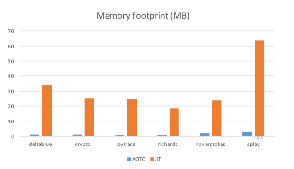
Figure 17: Memory comparison

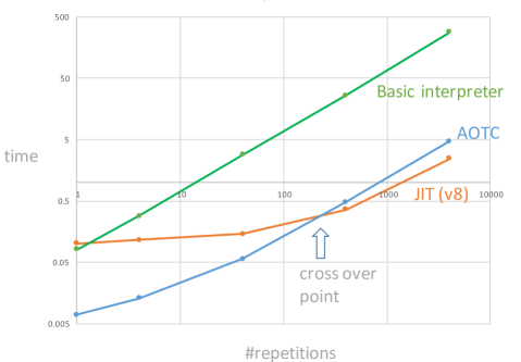
Figure 18: Running times for deltablue. Note the log-log scale.

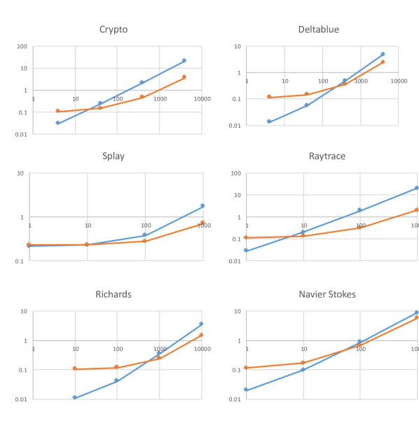
Figure 19: Crossover behavior of our AOTC system vs. the v8 runtime for the six Octane programs.

Interoperability. In a number of scenarios, it would be useful for compiled code from our JavaScript subset to interoperate with unrestricted JavaScript code. The most compelling case is to enable use of extant third-party libraries without having to port them, e.g., frameworks like jQuery for the web or the many libraries available for Node.js. Additionally, if a program contains dynamic code like that of Figure 14 or Figure 16, and that code is not performance-critical, it could be placed in an unrestricted JavaScript module rather than porting it.

Interoperability with unrestricted JavaScript entails a number of interesting tradeoffs. The simplest scheme would be to invoke unrestricted JavaScript from our subset (and vice versa) via a foreign function interface, with no shared heap. But, this would impose a high cost on such calls, due to marshalling of values, and could limit expressivity, e.g., passing functions would be difficult. Alternately, our JavaScript subset and unrestricted JavaScript could share the same heap, with additional type checks to ensure that inferred types are not violated by the unrestricted JavaScript. The type checks could “fail fast” at any violation, like in other work on gradual typing Rastogi et al. [2015]; Siek et al. [2015]; Vitousek et al. [2014]. But, this could lead to application behavior differing on our runtime versus a standard JavaScript runtime, as the standard runtime would not perform the additional checks. Without “fail fast,” the compiled code may need to be deoptimized at runtime type violations, adding significant complexity and potentially slowing down code with no type errors. At this point, we have a work-in-progress implementation of interoperability with a shared heap and “fail fast” semantics, but a robust implementation and proper evaluation of these tradeoffs remain as future work.

6 Related Work

Related work spans type systems and inference for JavaScript and dynamic languages in general, as well as the type inference literature more broadly.

Type systems and inference for JavaScript. Choi et al. Choi et al. [2015b, a] presented a typed subset of JavaScript for ahead-of-time compilation. Their work served as our starting point, and we built on it in two ways. First, our type system extends theirs with features that we found essential for real code, most crucially abstract types (see discussion throughout the paper). We also present a formalization and prove these extensions sound (Appendix B). Second, whereas they relied on programmer annotations to obtain types, we developed and implemented an automatic type inference algorithm.

Jensen et al. Jensen et al. [2009] present a type analysis for JavaScript based on abstract interpretation. They handle prototypal inheritance soundly. While their analysis could be adapted for compilation, it does not give a typing discipline. Moreover, their dataflow-based technique cannot handle partial programs, as discussed in Section 2.3.

TypeScript typ extends JavaScript with type annotations, aiming to expose bugs and improve developer productivity. To minimize adoption costs, its type system is very expressive but deliberately unsound. Further, it requires type annotations at function boundaries, while we do global inference. Flow flo is another recent type system for JavaScript, with an emphasis on effective flow-sensitive type inference. Although a detailed technical description is unavailable at the time of this writing, it appears that our inference technique has similarity to Flow’s in its use of upper- and -lower bound propagation Chaudhuri [2016]. Flow’s type language is similar to that of TypeScript, and it also sacrifices strict soundness in the interest of usability. It would be possible to create a sound gradually-typed version of Flow (i.e., one with dynamic type tests that may fail), but this would not enforce fixed object layout. For TypeScript, a sound gradually-typed variant already exists Rastogi et al. [2015], which we discuss shortly.

Early work on type inference for JavaScript by Thiemann Thiemann and Anderson et al. Anderson et al. ignored essential language features such as prototype inheritance, focusing instead on dynamic operations such as property addition. Guha et al. Guha et al. [2010] present a core calculus $\lambda_{\text{\it JS}}$ for JavaScript, upon which a number of type systems have been based. TeJaS Lerner et al. [2013] is a framework for building type checkers over $\lambda_{\text{\it JS}}$ using bidirectional type checking to provide limited inference. Politz et al. Politz et al. [2012] provide a type system enforcing access safety for a language with JavaScript-like dynamic property access.

Bhargavan et al. Bhargavan et al. [2013] develop a sound type system and inference for Defensive JavaScript (DJS), a JavaScript subset aimed at security embedding code in untrusted web pages. Unlike our work, DJS forbids prototype inheritance, and their type inference technique is not described in detail.

Gradual typing for JavaScript. Rastogi et al. Rastogi et al. [2012] give a constraint-based formulation of type inference for ActionScript, a gradually-typed class-based dialect of JavaScript. While they use many related techniques—their work and ours are inspired by Pottier cois Pottier [1998]—their gradually-typed setting leads to a very different constraint system. Their (sound) inference aims at proving runtime casts safe, so they need not validate upper bound constraints. They do not handle prototype inheritance, relying on ActionScript classes.

Rastogi et al. Rastogi et al. [2015] present Safe TypeScript, a sound, gradual type system for TypeScript. After running TypeScript’s (unsound) type inference, they run their (sound) type checker and insert runtime checks to ensure type safety. Richards et al. Richards et al. [2015] present StrongScript, another TypeScript extension with sound gradual typing. They allow the programmer to enforce soundness of some (but not all) type annotations using a specific type constructor, thus preserving some flexibility. They also use sound types to improve compilation and performance. Being based on TypeScript, both systems require type annotations, while we do not (except for signatures of external library functions). Moreover, they do not support general prototype inheritance or mutable methods, but rather rely on TypeScript’s classes and interfaces.

Type inference for other dynamic languages. Agesen et al. Agesen et al. [1993] present inference for Self, a key inspiration for JavaScript which includes prototype inheritance. Their constraint-based approach is inspired by Palsberg and Schwartzbach Palsberg and Schwartzbach [1991]. However, their notion of type is a set of values computed by data flow analysis, rather than syntactic typing discipline.

Foundations of type inference and constraint solving. Type inference has a long history, progressing from early work Damas and Milner [1982] through record calculi and row variables Wand [1987, 1989] through more modern presentations. Type systems for object calculi with object extension (e.g., prototype-based inheritance) and incomplete (abstract) objects extends back to the late 1990s Bono et al. [1996, 1997]; Rémy [1998]; Fisher and Mitchell [1995]. To our knowledge, our system is the first to describe inference for a language with both abstract objects and prototype inheritance.

Trifonov and Smith Trifonov and Smith [1996] describe constraint generation and solving in a core type system where (possibly recursive) types are generated by base types, $\bot$, $\top$ and $\rightarrow$ only. They introduce techniques for removing redundant constraints and optimizing constraint representation for faster type inference. Building on their work, Pottier cois Pottier [1998, 2001] crisply describes the essential ideas for subtyping constraint simplification and resolution in a similar core type system. We do not know of any previous generalization of this work that handles prototype inheritance. In both of these systems, lower and upper bounds for each type variable are already defined while resolving and simplifying constraints. Both lines of work support partial programs, producing schemas with arbitrary constraints rather than an established style of polymorphic type.

Pottier and Rémy cois Pottier and Rémy [2005] describe type inference for ML, including records, polymorphism, and references. Rémy and Vouillon Rémy and Vouillon [1998] describe type inference for class-based objects in Objective ML. These approaches are based on row polymorphism rather than subtyping, and they do not handle prototype inheritance or non-explicit subtyping.

Aiken Aiken [1999] gives an overview of program analysis in the general framework of set constraints, with applications to dataflow analysis and simple type inference. Most of our constraints would fit in his framework with little adaptation, and his resolution method also uses lower and upper bounds. His work is general and does not look into specific program construct details like objects, or a specific language like JavaScript.

Appendix A A developer-centric view

In this section, we give a developer-centric view of our JavaScript subset, without resorting to details of type inference. We produced similar documentation for the developer team who created the native Tizen applications discussed in Section 5.

From a developer’s perspective, our subset restricts JavaScript in the following ways:

1. Each variable, object property, or parameter can be assigned values only of a single type throughout the execution. Here, type denotes distinct categories of values, such as numbers, booleans, strings, and objects.

2. An object’s type depends on the set of properties it contains. It is acceptable to supply an object with more properties in a context in which an object type with fewer properties was expected, as long as the types of common properties are the same (akin to “upcasting”); however, the other way around (“downcasting”) is not allowed.

3. Although JavaScript makes little distinction between use of objects as records, maps, and arrays, our subset does. Record usage is suitable when the set of properties is known ahead of time and fixed. Map usage is suitable when the set of properties (or “keys”) can be added and deleted; however, the values stored against those keys must all be of a common type. Arrays are indexed with numeric indices, as opposed to maps which are indexed by string indices. We use the [] accessor for maps and arrays, while the ’.’ accessor is only for structs. Moreover, iteration is only supported over maps and arrays; it is not possible to iterate over properties of a record using a for-in loop.

4. When using objects as records, properties cannot be added or removed after creation. This means that all the properties needed on that object throughout the execution of the program should be defined in the corresponding constructor or object literal.

5. Properties inherited via prototype inheritance are read only, that is, they cannot be modified using a reference to the inheritor. (They can still be modified using a reference to the prototype.) If a method in a prototype writes to a property, the property must be re-declared in the inheritor.

6. Prototype inheritance can be carried out only from a variable whose provenance does not include an intervening (implicit) upcast. That is to say, the object type of the variable should coincide with the actual runtime value that that variable holds.

7. Although built-in types such as Array and String are available for use, their properties cannot be “monkey patched” using assignment to the corresponding prototypes.

8. eval and with are not supported, and neither is the arguments array. Low-level ways of manipulating functions as objects are also not supported.

The above discipline has to be followed statically. Code such as var v = false ? "hello" : 1 is not acceptable, even though at runtime v can only hold a numeric value. The type checker will reject a program if it cannot statically reason about the safety of the program, though sometimes it may appear to be overly conservative.

Appendix B Type system metatheory

This section presents the full type system in Figure 20, along with a full proof of soundness of our type inference (proof of Theorem 1), an extension to handle recursive types, and a proof of soundness of the type system.

Figure 21 shows constraint generation rules for handling of first-class functions, which were omitted from Figure 8. Bound propagation and ascription can be extended to function types in a way similar to method types.

T-Int $$\displaystyle{\hbox{}\over\hbox{\hskip 26.76672pt\vbox{\vbox{}\hbox{\hskip-26.76671pt\hbox{\hbox{$\displaystyle\displaystyle R,\Gamma\vdash n:\mathsf{int}$}}}}}} \displaystyle{\hbox{\hskip 18.72392pt\vbox{\hbox{\hskip-18.72392pt\hbox{\hbox{$\displaystyle\displaystyle\Gamma(x)=\tau$}}}\vbox{}}}\over\hbox{\hskip 24.22557pt\vbox{\vbox{}\hbox{\hskip-24.22556pt\hbox{\hbox{$\displaystyle\displaystyle R,\Gamma\vdash x:\tau$}}}}}} \displaystyle{\hbox{\hskip 69.86934pt\vbox{\hbox{\hskip-69.86932pt\hbox{\hbox{$\displaystyle\displaystyle\Gamma(x)=\tau_{1}\quad R,\Gamma\vdash e:\tau\quad\tau\ \mathsf{<:}\ \tau_{1}$}}}\vbox{}}}\over\hbox{\hskip 34.6092pt\vbox{\vbox{}\hbox{\hskip-34.60919pt\hbox{\hbox{$\displaystyle\displaystyle R,\Gamma\vdash x:=e:\tau$}}}}}} \displaystyle{\hbox{\hskip 118.80107pt\vbox{\hbox{\hskip-118.80107pt\hbox{\hbox{$\displaystyle\displaystyle R,\Gamma\left[x\mapsto\tau_{1}\right]\vdash e_{1}:\sigma_{1}\quad\Vdash\tau_{1}\quad\sigma_{1}\ \mathsf{<:}\ \tau_{1}$}\hskip 20.00003pt\hbox{\hbox{$\displaystyle\displaystyle R,\Gamma\left[x\mapsto\tau_{1}\right]\vdash e_{2}:\tau$}}}}\vbox{}}}\over\hbox{\hskip 50.28787pt\vbox{\vbox{}\hbox{\hskip-50.28786pt\hbox{\hbox{$\displaystyle\displaystyle R,\Gamma\vdash\mathsf{let}~{}x=e_{1}~{}\mathsf{in}~{}e_{2}:\tau$}}}}}} \displaystyle{\hbox{}\over\hbox{\hskip 25.31477pt\vbox{\vbox{}\hbox{\hskip-25.31476pt\hbox{\hbox{$\displaystyle\displaystyle\nu,\Gamma\vdash\mathsf{this}:\nu$}}}}}} \displaystyle{\hbox{\hskip 51.84563pt\vbox{\hbox{\hskip-51.84563pt\hbox{\hbox{$\displaystyle\displaystyle\top,\Gamma\left[x\mapsto\tau_{1}\right]\vdash e:\tau_{2}\quad\Vdash\tau_{1}$}}}\vbox{}}}\over\hbox{\hskip 67.20863pt\vbox{\vbox{}\hbox{\hskip-67.20862pt\hbox{\hbox{$\displaystyle\displaystyle R,\Gamma\vdash\mathsf{function}\left(x:\tau_{1}\right)\left\{e\right\}:\tau_{1}\rightarrow\tau_{2}$}}}}}} \displaystyle{\hbox{\hskip 49.03778pt\vbox{\hbox{\hskip-49.03777pt\hbox{\hbox{$\displaystyle\displaystyle\nu,\Gamma\left[x\mapsto\tau_{1}\right]\vdash e:\tau_{2}\quad\Vdash\tau_{1}$}}}\vbox{}}}\over\hbox{\hskip 73.56747pt\vbox{\vbox{}\hbox{\hskip-73.56746pt\hbox{\hbox{$\displaystyle\displaystyle R,\Gamma\vdash\mathsf{function}\left(x:\tau_{1}\right)\left\{e\right\}:\left[\nu\right]\tau_{1}\Rightarrow\tau_{2}$}}}}}} \displaystyle{\hbox{\hskip 88.7384pt\vbox{\hbox{\hskip-88.7384pt\hbox{\hbox{$\displaystyle\displaystyle R,\Gamma\vdash e_{1}:\tau_{3}\rightarrow\tau$}\hskip 20.00003pt\hbox{\hbox{$\displaystyle\displaystyle R,\Gamma\vdash e_{2}:\tau_{2}\quad\tau_{2}\ \mathsf{<:}\ \tau_{3}$}}}}\vbox{}}}\over\hbox{\hskip 31.32425pt\vbox{\vbox{}\hbox{\hskip-31.32423pt\hbox{\hbox{$\displaystyle\displaystyle R,\Gamma\vdash e_{1}\left(e_{2}\right):\tau$}}}}}} \displaystyle{\hbox{\hskip 35.55249pt\vbox{\hbox{\hskip-35.55249pt\hbox{\hbox{$\displaystyle\displaystyle\tau\ \mathsf{<:}\ \left\{\langle\ \rangle\mid\langle\ \rangle\right\}^{\mathbf{NA}}$}}}\vbox{}}}\over\hbox{\hskip 26.78468pt\vbox{\vbox{}\hbox{\hskip-26.78468pt\hbox{\hbox{$\displaystyle\displaystyle R,\Gamma\vdash\mathsf{null}:\tau$}}}}}} \displaystyle{\hbox{\hskip 108.5956pt\vbox{\hbox{\hskip-108.5956pt\hbox{\hbox{$\displaystyle\displaystyle\tau_{1}\ \mathsf{<:}\ \left\{\langle a:\tau\rangle\mid\langle\ \rangle\right\}^{\mathbf{NA}}$}\hskip 20.00003pt\hbox{\hbox{$\displaystyle\displaystyle R,\Gamma\vdash e:\tau_{1}\quad\tau\neq\left[\cdot\right]\tau_{2}\Rightarrow\tau_{3}$}}}}\vbox{}}}\over\hbox{\hskip 28.56122pt\vbox{\vbox{}\hbox{\hskip-28.5612pt\hbox{\hbox{$\displaystyle\displaystyle R,\Gamma\vdash e.a:\tau$}}}}}} \displaystyle{\hbox{\hskip 72.84123pt\vbox{\hbox{\hskip-72.84122pt\hbox{\hbox{$\displaystyle\displaystyle R,\Gamma\vdash_{AU}\tau_{b}.a:=e:\tau\quad R,\Gamma\vdash e_{1}:\tau_{b}$}}}\vbox{}}}\over\hbox{\hskip 40.34485pt\vbox{\vbox{}\hbox{\hskip-40.34485pt\hbox{\hbox{$\displaystyle\displaystyle R,\Gamma\vdash e_{1}.a:=e:\tau$}}}}}} \displaystyle{\hbox{\hskip 143.78627pt\vbox{\hbox{\hskip-143.78627pt\hbox{\hbox{$\displaystyle\displaystyle R,\Gamma\vdash e_{1}:\tau_{1}\quad R,\Gamma\vdash e_{2}:\tau_{2}$}\hskip 20.00003pt\hbox{\hbox{$\displaystyle\displaystyle\tau_{1}\ \mathsf{<:}\ \left\{\langle a:\left[\cdot\right]\tau_{3}\Rightarrow\tau\rangle\mid\langle\ \rangle\right\}^{\mathbf{NC}}\quad\tau_{2}\ \mathsf{<:}\ \tau_{3}$}}}}\vbox{}}}\over\hbox{\hskip 36.18939pt\vbox{\vbox{}\hbox{\hskip-36.18939pt\hbox{\hbox{$\displaystyle\displaystyle R,\Gamma\vdash e_{1}.a\left(e_{2}\right):\tau$}}}}}} \displaystyle{\hbox{}\over\hbox{\hskip 54.1768pt\vbox{\vbox{}\hbox{\hskip-54.17679pt\hbox{\hbox{$\displaystyle\displaystyle R,\Gamma\vdash\left\{\cdot\right\}:\left\{\langle\ \rangle\mid\langle\ \rangle\right\}^{\mathbf{P}\left(\langle\ \rangle,\langle\ \rangle\right)}$}}}}}} \displaystyle{\hbox{\hskip 193.46964pt\vbox{\hbox{\hskip-10.32431pt\hbox{\hbox{$\displaystyle\displaystyle\Vdash\rho^{q}$}}}\vbox{\hbox{\hskip-181.83415pt\hbox{\hbox{$\displaystyle\displaystyle\rho=\left\{r\mid w\right\}$}\hskip 20.00003pt\hbox{\hbox{$\displaystyle\displaystyle q={\mathbf{P}\left(mr,mw\right)}$}\hskip 20.00003pt\hbox{\hbox{$\displaystyle\displaystyle R,\Gamma\vdash e_{p}:{\left\{r_{p}\mid w_{p}\right\}}^{{\mathbf{P}\left(mr_{p},mw_{p}\right)}}$}\hskip 20.00003pt\hbox{\hbox{$\displaystyle\displaystyle w=\langle a_{1}:\tau_{1},\ldots,a_{n}:\tau_{n}\rangle\quad$}}}}}}\vbox{\hbox{\hskip-193.46962pt\hbox{\hbox{$\displaystyle\displaystyle\forall i\in 1..n.~{}R,\Gamma\vdash_{AU}\rho^{q}.a_{i}:=e_{i}:\sigma_{i}\wedge\sigma_{i}\ \mathsf{<:}\ \tau_{i}$}\hskip 20.00003pt\hbox{\hbox{$\displaystyle\displaystyle{r_{p}\cup w}={r}$}\hskip 20.00003pt\hbox{\hbox{$\displaystyle\displaystyle mr\ \mathsf{<:}\ mr_{p}$}\hskip 20.00003pt\hbox{\hbox{$\displaystyle\displaystyle mw\ \mathsf{<:}\ mw_{p}$}}}}}}\vbox{}}}}}\over\hbox{\hskip 75.32672pt\vbox{\vbox{}\hbox{\hskip-75.32672pt\hbox{\hbox{$\displaystyle\displaystyle R,\Gamma\vdash\left\{a_{1}:e_{1},\ldots,a_{n}:e_{n}\right\}_{\rho^{q}}~{}\textsf{proto}~{}e_{p}:\rho^{q}$}}}}}} \displaystyle{\hbox{\hskip 142.62968pt\vbox{\hbox{\hskip-142.62967pt\hbox{\hbox{$\displaystyle\displaystyle\tau_{b}\ \mathsf{<:}\ \left\{\langle a:\tau_{f}\rangle\mid\langle a\rangle\right\}^{\mathbf{NA}}$}\hskip 20.00003pt\hbox{\hbox{$\displaystyle\displaystyle R,\Gamma\vdash e:\tau$}\hskip 20.00003pt\hbox{\hbox{$\displaystyle\displaystyle\tau\neq\left[\tau_{x}\right]\tau_{y}\Rightarrow\tau_{z}$}\hskip 20.00003pt\hbox{\hbox{$\displaystyle\displaystyle\tau\ \mathsf{<:}\ \tau_{f}$}}}}}}\vbox{}}}\over\hbox{\hskip 42.93234pt\vbox{\vbox{}\hbox{\hskip-42.93234pt\hbox{\hbox{$\displaystyle\displaystyle R,\Gamma\vdash_{AU}\tau_{b}.a:=e:\tau$}}}}}} \displaystyle{\hbox{\hskip 175.2453pt\vbox{\hbox{\hskip-57.54488pt\hbox{\hbox{$\displaystyle\displaystyle\tau_{b}\ \mathsf{<:}\ \left\{\langle a:\left[\cdot\right]\tau_{1}\Rightarrow\tau_{2}\rangle\mid\langle a\rangle\right\}^{\mathbf{NA}}$}}}\vbox{\hbox{\hskip-175.24529pt\hbox{\hbox{$\displaystyle\displaystyle R,\Gamma\vdash e:\left[\left\{r_{r}\mid w_{r}\right\}^{\mathbf{NC}}\right]\tau_{1}\Rightarrow\tau_{2}$}\hskip 20.00003pt\hbox{\hbox{$\displaystyle\displaystyle\tau_{b}=\rho^{q}\quad q={\mathbf{P}\left(mr,mw\right)}$}\hskip 20.00003pt\hbox{\hbox{$\displaystyle\displaystyle mr\ \mathsf{<:}\ r_{r}\quad mw\ \mathsf{<:}\ w_{r}$}}}}}\vbox{}}}}\over\hbox{\hskip 75.83119pt\vbox{\vbox{}\hbox{\hskip-75.83119pt\hbox{\hbox{$\displaystyle\displaystyle R,\Gamma\vdash_{AU}\tau_{b}.a:=e:\left[\left\{r_{r}\mid w_{r}\right\}^{\mathbf{NC}}\right]\tau_{1}\Rightarrow\tau_{2}$}}}}}}$$       T-Var        T-VarUpd        T-VarDecl        T-This        T-Fun        T-Meth        T-FCall        T-Null        T-Attr        T-AttrUpd        T-MCall        T-Emp        T-ObjLit        T-AttrUpdV        T-AttrUpdM 

Figure 20: Typing judgement.

C-FunDecl $$\displaystyle{\hbox{\hskip 131.07153pt\vbox{\hbox{\hskip-131.07153pt\hbox{\hbox{$\displaystyle\displaystyle\mathsf{fresh}~{}X_{1},Y,X_{{\kern-0.5833pt}R},X\quad\mathsf{!}~{}\mathsf{has\_this(}e\mathsf{)}$}\hskip 20.00003pt\hbox{\hbox{$\displaystyle\displaystyle X_{{\kern-0.5833pt}R},\Gamma\left[x\mapsto X_{1}\right]\vdash e:Y\mid C$}}}}\vbox{}}}\over\hbox{\hskip 128.65546pt\vbox{\vbox{}\hbox{\hskip-128.65544pt\hbox{\hbox{$\displaystyle\displaystyle\begin{array}[]{l@{~}c@{~}l}R,\Gamma\vdash\mathsf{function}\left(x\right)\left\{e\right\}:X\mid\hfil~{}&\hfil~{}&C\wedge X_{{\kern-0.5833pt}R}^{\mathsf{r}}\equiv\langle\ \rangle\@arraycr&\wedge&X^{\mathsf{r}}\equiv(X_{1}\rightarrow Y)\end{array}$}}}}}} \displaystyle{\hbox{\hskip 114.83418pt\vbox{\hbox{\hskip-114.83417pt\hbox{\hbox{$\displaystyle\displaystyle\mathsf{fresh}~{}X_{3},X$}\hskip 20.00003pt\hbox{\hbox{$\displaystyle\displaystyle R,\Gamma\vdash e_{1}:X_{1}\mid C_{1}\qquad R,\Gamma\vdash e_{2}:X_{2}\mid C_{2}$}}}}\vbox{}}}\over\hbox{\hskip 153.73218pt\vbox{\vbox{}\hbox{\hskip-153.73216pt\hbox{\hbox{$\displaystyle\displaystyle\begin{array}[]{l@{~}c@{~}l}R,\Gamma\vdash e_{1}\left(e_{2}\right):X\mid\hfil~{}&\hfil~{}&C_{1}\wedge C_{2}\wedge X_{1}^{\mathsf{r}}\equiv(X_{3}\rightarrow X)\@arraycr&&\wedge X_{2}^{\mathsf{r}}\ \mathsf{<:}\ X_{3}^{\mathsf{r}}\wedge X_{2}^{\mathsf{w}}\ \mathsf{<:}\ X_{3}^{\mathsf{w}}\end{array}$}}}}}}$$        C-FunApp

Figure 21: Constraint generation rules for functions.

B.1 Soundness of type inference

B.1.1 Proof of Lemma 1

Proof.

Let us consider a constraint $C\in\mathcal{C}$, by Rule (i), $C\in\mathcal{C}^{\prime}$. The proof proceeds by case analysis over the form of the constraint $C$. Note that Rules (xiv)-(xvi), not essential for soundness, are indeed not used in the proof.

• If $C$ is of the form $X^{s}\ \mathsf{<:}\ L$, then by Rule (iii), $L\in\left\lceil{X^{s}}\right\rceil$. Therefore $\Phi(X^{s})=\mathsf{glb}(\left\lceil{X^{s}}\right\rceil)\ \mathsf{<:}\ L$ (see 1, Line 6).

• If $C$ is of the form $L\ \mathsf{<:}\ X^{s}$, then by Rule (iv), $L\in\left\lfloor{X^{s}}\right\rfloor$. At type ascription (Line 8) we checked that $L\ \mathsf{<:}\ \Phi(X^{s})$.

• If $C$ is of the form $X^{s}\ \mathsf{<:}\ Y^{t}$, then by Rule (v), $\left\lfloor{X^{s}}\right\rfloor\subseteq\left\lfloor{Y^{t}}\right\rfloor$ and $\left\lceil{Y^{t}}\right\rceil\subseteq\left\lceil{X^{s}}\right\rceil$. Note that by Rules (vii) and (viii), either both $\left\lceil{X^{s}}\right\rceil$ and $\left\lfloor{X^{s}}\right\rfloor$ are empty, or both are non-empty, and similarly for $\left\lceil{Y^{t}}\right\rceil$ and $\left\lfloor{Y^{t}}\right\rfloor$.

  • If $\left\lfloor{X^{s}}\right\rfloor=\left\lceil{X^{s}}\right\rceil=\emptyset$ then $\left\lceil{Y^{t}}\right\rceil=\emptyset$ thus $\left\lfloor{Y^{t}}\right\rfloor=\emptyset$ and $\Phi(X^{s})=\mathsf{default}\ \mathsf{<:}\ \mathsf{default}=\Phi(Y^{t})$.

  • Symmetrically, if $\left\lfloor{Y^{t}}\right\rfloor=\left\lceil{Y^{t}}\right\rceil=\emptyset$ then $\left\lfloor{X^{s}}\right\rfloor=\emptyset$ therefore $\left\lceil{X^{s}}\right\rceil=\emptyset$ and $\Phi(X^{s})=\mathsf{default}\ \mathsf{<:}\ \mathsf{default}=\Phi(Y^{t})$.

  • Otherwise $\left\lceil{X^{s}}\right\rceil$ and $\left\lceil{Y^{t}}\right\rceil$ are both non-empty, thus $\Phi(X^{s})=\mathsf{glb}(\left\lceil{X^{s}}\right\rceil)\ \mathsf{<:}\ \mathsf{glb}(\left\lceil{Y^{t}}\right\rceil)=\Phi(Y^{t})$ since $\left\lceil{X^{s}}\right\rceil\subseteq\left\lceil{Y^{t}}\right\rceil$.

• If $C$ is of the form $X^{s}\ \mathsf{<:}\ Y^{t}\backslash\{a_{1},\ldots,a_{n}\}$, then $\langle\ \rangle\in\left\lceil{X^{s}}\right\rceil$ and $\langle\ \rangle\in\left\lceil{Y^{t}}\right\rceil$, i.e., $\Phi(X^{s})$ and $\Phi(Y^{t})$ are rows. This is because such a constraint is always generated along with a constraint $Y^{\mathsf{w}}\ \mathsf{<:}\ \langle a_{1}:X_{1},\ldots,a_{n}:X_{n}\rangle$ (see Rule [C-ObjLit]), and by Rules (ii), (v), (vii) and (viii). But by Rule (vi), $\{\langle F\rangle\backslash\{a_{1},\ldots,a_{n}\}\ |\ \langle F\rangle\in\left\lceil{Y^{t}}\right\rceil\}\subseteq\left\lceil{X^{s}}\right\rceil$, therefore $\Phi(X^{s})=\mathsf{glb}(\left\lceil{X^{s}}\right\rceil)\ \mathsf{<:}\ \mathsf{glb}(\left\lceil{Y^{t}}\right\rceil)\backslash\{a_{1},\ldots,a_{n}\}=\Phi(Y^{s})\backslash\{a_{1},\ldots,a_{n}\}$.

• If $C$ is of the form $\mathsf{proto}(X)$, then $\langle\ \rangle\in\left\lceil{X^{\mathsf{r}}}\right\rceil$ since $\mathsf{proto}(X)$ is always generated along with a row constraint on $X^{\mathsf{r}}$ (rules [C-ObjEmp] and [C-ObjLit]; also true if $\mathsf{proto}(X)$ was generated using Rule (ix), by induction on the number of uses of Rule (ix)). At type ascription (Lines 15 and 18), $\Phi(X)$ is a prototypal type.

• If $C$ is of the form $\mathsf{concrete}\!\left(X\right)$, then $\langle\ \rangle\in\left\lceil{X^{\mathsf{r}}}\right\rceil$ since $\mathsf{proto}(X)$ is always generated along with a row constraint on $X^{\mathsf{r}}$ (rules [C-MethApp]; also true if $\mathsf{proto}(X)$ was generated using Rule (x), by induction on the number of uses of Rule (x)).

  • if $\mathsf{proto}(X)\ \in\mathcal{C}^{\prime}$, then by Rule (xi) and the case $X^{s}\ \mathsf{<:}\ Y^{t}$, $\Phi(X^{\mathsf{r}})\ \mathsf{<:}\ \Phi(X^{\mathsf{mr}})$ and $\Phi(X^{\mathsf{w}})\ \mathsf{<:}\ \Phi(X^{\mathsf{mw}})$, therefore $\Phi(X)=\left\{\Phi(X^{\mathsf{r}})\mid\Phi(X^{\mathsf{w}})\right\}^{\mathbf{P}\left(\Phi(X^{\mathsf{mr}}),\Phi(X^{\mathsf{mw}})\right)}$ is concrete (Lines 15 and 18).

  • otherwise $\Phi(X)$ is of the form $\rho^{\mathbf{NC}}$, thus concrete (Lines 15 and 19).

• if $C$ is of the form $\mathsf{strip}(X)$, then $\left\lceil{X^{\mathsf{r}}}\right\rceil$ contains a method type since $\mathsf{strip}(X)$ is always generated along with a method constraint on $X^{\mathsf{r}}$. By type ascription (Lines 2 and 13), $X$ is assigned an attached method type (of the form $\left[\cdot\right]\tau_{1}\Rightarrow\tau_{2}$, i.e., without a receiver type), and therefore $\Phi$ satisfies constraint $C$.

• If $C$ is of the form $\mathsf{attach}(X_{b},X_{f},X_{v})$, then if $\Phi(X_{v})$ is not a method type, the result is trivial. Otherwise, by definition of ascription (Line 11), there must exist an $\left[X_{{\kern-0.5833pt}R}\right]Y_{1}\Rightarrow Y_{2}\in\left\lceil{X^{\mathsf{r}}_{v}}\right\rceil$. Using Rule (xii), $\mathsf{proto}(X_{b})\ \in\mathcal{C}^{\prime}$, $X_{b}^{\mathsf{mr}}\ \mathsf{<:}\ T^{\mathsf{r}}\ \in\mathcal{C}^{\prime}$, $X_{b}^{\mathsf{mw}}\ \mathsf{<:}\ T^{\mathsf{w}}\ \in\mathcal{C}^{\prime}$, and $\mathsf{strip}(X_{f})\ \in\mathcal{C}^{\prime}$. Therefore, using the previous cases of this lemma, the assignment $\Phi$ satisfies constraint $C$.

• if $C$ is any acceptance criterion ($\mathsf{notmethod}(X)$ or $\mathsf{notproto}(X)$), we do an explicit check during ascription (Lines 12 and 17), thereby ensuring that $\Phi$ satisfies constraint $C$.

∎

B.1.2 Proof of Lemma 2

Proof.

We proceed by case analysis on $\Phi(X^{\mathsf{r}})$, $\Phi(Y^{\mathsf{r}})$, and the possible constraints on $X$ and $Y$. By Lemma 1, $\Phi(X^{\mathsf{r}})\ \mathsf{<:}\ \Phi(Y^{\mathsf{r}})$ and $\Phi(X^{\mathsf{w}})\ \mathsf{<:}\ \Phi(Y^{\mathsf{w}})$.

If $\Phi(Y^{\mathsf{r}})$ is a base or function type, then $\Phi(X^{\mathsf{r}})=\Phi(Y^{\mathsf{r}})$ since there is no subtyping between those types and by rules (v), (vii) and (viii). By definition of ascription $\Phi(X)=\Phi(Y)$.

If $\Phi(Y^{\mathsf{r}})$ is a method type $\left[\tau_{r}\right]\tau_{1}\Rightarrow\tau_{2}$, then by definition of ascription, as well as Rules (v), (vii) and (viii), $\Phi(X^{\mathsf{r}})=\Phi(Y^{\mathsf{r}})$. Three cases arise.

• If $\mathsf{strip}(X)\ \in\mathcal{C}^{\prime}$ then by Rule (xiii), $\mathsf{strip}(Y)\ \in\mathcal{C}^{\prime}$. Therefore by definition of ascription (Line 2 and 13), $\Phi(X)=\left[\cdot\right]\tau_{1}\Rightarrow\tau_{2}=\Phi(Y)$.

• Otherwise, if $\mathsf{strip}(Y)\ \in\mathcal{C}^{\prime}$, then by definition of ascription (Lines 2 and 13), $\Phi(X)=\left[\tau_{r}\right]\tau_{1}\Rightarrow\tau_{2}\ \mathsf{<:}\ \left[\cdot\right]\tau_{1}\Rightarrow\tau_{2}=\Phi(Y)$ by subtyping rule [S-Method] (Figure 5).

• Otherwise, by definition of ascription (Line 13), $\Phi(X)=\left[\tau_{r}\right]\tau_{1}\Rightarrow\tau_{2}=\Phi(Y)$.

Otherwise $\Phi(Y^{\mathsf{r}})$ is a row and $\langle\ \rangle\in\left\lceil{Y^{\mathsf{r}}}\right\rceil$.

• If $\mathsf{proto}(Y)\ \in\mathcal{C}^{\prime}$ then by Rule (ix)$,\mathsf{proto}(X)\ \in\mathcal{C}^{\prime}$ and $\forall s,X^{s}\equiv Y^{s}\ \in\mathcal{C}^{\prime}$, hence by Lemma 1, $\forall s,\Phi(X^{s})=\Phi(Y^{s})$. Therefore by definition of ascription (Lines 15 and 18), $\Phi(X)=\Phi(Y)$.

• Otherwise, if $\mathsf{concrete}\!\left(Y\right)\ \in\mathcal{C}^{\prime}$, then by Rule (x), we get $\mathsf{concrete}\!\left(X\right)\ \in\mathcal{C}^{\prime}$. By definition of ascription, $\Phi(Y)=\left\{\Phi(Y^{\mathsf{r}})\mid\Phi(Y^{\mathsf{w}})\right\}^{\mathbf{NC}}$, and

  • either $\Phi(X)=\left\{\Phi(X^{\mathsf{r}})\mid\Phi(X^{\mathsf{w}})\right\}^{\mathbf{NC}}$;

  • or $\Phi(X)=\left\{\Phi(X^{\mathsf{r}})\mid\Phi(X^{\mathsf{w}})\right\}^{\mathbf{P}\left(\Phi(X^{\mathsf{mr}}),\Phi(X^{\mathsf{mw}})\right)}$, with $\Phi(X^{\mathsf{r}})\ \mathsf{<:}\ \Phi(X^{\mathsf{mr}})$ and $\Phi(X^{\mathsf{w}})\ \mathsf{<:}\ \Phi(X^{\mathsf{mw}})$ by Rule (xi) and Lemma 1).

  In both cases $\Phi(X)\ \mathsf{<:}\ \Phi(Y)$.

• Otherwise we have $\Phi(Y)=\left\{\Phi(Y^{\mathsf{r}})\mid\Phi(Y^{\mathsf{w}})\right\}^{\mathbf{NA}}$, and also $\Phi(X)\ \mathsf{<:}\ \left\{\Phi(X^{\mathsf{r}})\mid\Phi(X^{\mathsf{w}})\right\}^{\mathbf{NA}}$, therefore $\Phi(X)\ \mathsf{<:}\ \Phi(Y)$.

∎

B.1.3 Proof of Lemma 3

Proof.

Following the definition of $\Vdash\tau$ in Figure 5, if $\Phi(X)$ is a non-object type then the result is trivial.

Otherwise, $\Phi(X)$ is of the form $\left\{\sf r\mid\sf w\right\}^{q}$. By Rule (ii), $X^{\mathsf{all}}\ \mathsf{<:}\ X^{\mathsf{r}}\ \mathsf{<:}\ X^{\mathsf{w}}\ \in\mathcal{C}^{\prime}$ and $X^{\mathsf{all}}\ \mathsf{<:}\ X^{\mathsf{mr}}\ \mathsf{<:}\ X^{\mathsf{mw}}\ \in\mathcal{C}^{\prime}$, therefore by Lemma 1 and ascription, there exist rows $\Phi(X^{\mathsf{all}})$, $\Phi(X^{\mathsf{r}})$, $\Phi(X^{\mathsf{w}})$, $\Phi(X^{\mathsf{mr}})$ and $\Phi(X^{\mathsf{mw}})$ such that $\Phi(X^{\mathsf{all}})\ \mathsf{<:}\ \Phi(X^{\mathsf{r}})\ \mathsf{<:}\ \Phi(X^{\mathsf{w}})$ and $\Phi(X^{\mathsf{all}})\ \mathsf{<:}\ \Phi(X^{\mathsf{mr}})\ \mathsf{<:}\ \Phi(X^{\mathsf{mw}})$. By type ascription (Line 15), ${\sf r}=\Phi(X^{\mathsf{r}})\ \mathsf{<:}\ \Phi(X^{\mathsf{w}})={\sf w}$.

Moreover, if $q$ is of the form ${\mathbf{P}\left(\sf mr,\sf mw\right)}$, then by type ascription (Line 18), ${\sf mr}=\Phi(X^{\mathsf{mr}})\ \mathsf{<:}\ \Phi(X^{\mathsf{mw}})={\sf mw}$. Finally, $\Phi(X^{\mathsf{all}})\ \mathsf{<:}\ \Phi(X^{\mathsf{r}})={\sf r}$, therefore $\forall a\in\mathsf{dom(}{\sf r}\mathsf{)},{\sf r}[a]=\Phi(X^{\mathsf{all}})[a]$. Similarly, $\Phi(X^{\mathsf{all}})\ \mathsf{<:}\ \Phi(X^{\mathsf{mr}})={\sf mr}$, therefore $\forall a\in\mathsf{dom(}{\sf mr}\mathsf{)},{\sf mr}[a]=\Phi(X^{\mathsf{all}})[a]$. Therefore, $\forall a\in\mathsf{dom(}{\sf mr}\mathsf{)}\cap\mathsf{dom(}{\sf r}\mathsf{)},{\sf mr}[a]=\Phi(X^{\mathsf{all}})[a]={\sf r}[a]$. ∎

B.1.4 Proof of Theorem 1

Proof.

The proof proceeds by induction on the structure of the constraint-generating relation. For ease of reference, we label the hypotheses as follows:

• H1: $X_{{\kern-0.5833pt}R},\Gamma\vdash e:X\mid C$

• H2: $\Phi\vdash C$

The cases C-Var and C-This follow directly from H1 and H2, using typing rules T-Var and T-This, respectively.

C-Int: Since $X^{\mathsf{r}}\equiv\mathsf{int}\ \in\mathcal{C}^{\prime}$, by definition of ascription (Line 10), $\Phi(X)=\mathsf{int}$ and we conclude using T-Int.

C-ObjEmp: Similarly, since $\mathsf{proto}(X)\ \in\mathcal{C}^{\prime}$, $X^{\mathsf{r}}\equiv\langle\ \rangle\ \in\mathcal{C}^{\prime}$ and $X^{\mathsf{w}}\equiv\langle\ \rangle\ \in\mathcal{C}^{\prime}$, by Rule (ii) and defintion of ascription (Line 16), $\Phi(X)=\left\{\langle\ \rangle\mid\langle\ \rangle\right\}^{\mathbf{P}\left(\langle\ \rangle,\langle\ \rangle\right)}$ and we conclude using T-ObjEmp.

C-Null: Since $X^{\mathsf{w}}\ \mathsf{<:}\ \langle\ \rangle\ \in\mathcal{C}^{\prime}$, by definition of ascription (Lines 15–20), $\Phi(X)$ is an object type and we conclude using T-Null, and the subtyping rules of Figure 5.

C-VarDecl: From the induction hypothesis, we have that

• $\Phi(X_{{\kern-0.5833pt}R}),\Phi(\Gamma\left[x\mapsto\Phi(X_{1})\right])\vdash e_{1}:\Phi(Y_{1})$

• $\Phi(X_{{\kern-0.5833pt}R}),\Phi(\Gamma\left[x\mapsto\Phi(X_{1})\right])\vdash e_{2}:\Phi(X)$.

Moreover, since $Y^{\mathsf{r}}_{1}\ \mathsf{<:}\ X^{\mathsf{r}}_{1}\ \in\mathcal{C}^{\prime}$ and $Y^{\mathsf{w}}_{1}\ \mathsf{<:}\ X^{\mathsf{w}}_{1}\ \in\mathcal{C}^{\prime}$, by Lemma 2 we get $\Phi(Y_{1})\ \mathsf{<:}\ \Phi(X_{1})$; and Lemma 3 ensures that $\Vdash\Phi(X_{1})$ Hence, T-VarDecl types $e$ at $\Phi(X)$.

C-VarUpd, C-FunDecl, C-MethDecl, C-Attr: As with C-VarDecl, these cases follow from a straightforward application of the induction hypothesis, as well as Lemmas 2 and 3.

C-FunApp and C-MethApp: Follow from the hypotheses (including the induction hypothesis) and the definition of the subtyping relation, as well as Lemmas 2 and 3.

C-AttrUpd: There are two cases for attribute update: the expression being attached is or is not ascribed a detached method type. This two cases correspond respectively to typing rules T-AttrUpdM and T-AttrUpdV.

More precisely, from the hypothesis of C-AttrUpd and induction hypothesis, we have that $\Phi(X_{{\kern-0.5833pt}R}),\Phi(\Gamma)\vdash e_{1}:\Phi(X_{b})$ and $\Phi(X_{{\kern-0.5833pt}R}),\Phi(\Gamma)\vdash e_{2}:\Phi(X_{v})$. From the constraints and Lemma 2, we have that $\Phi(X_{v})\ \mathsf{<:}\ \Phi(X_{f})$; and by Lemma 1 and definition of type ascription on constraint $X^{\mathsf{w}}_{b}\ \mathsf{<:}\ \langle a:X_{f}\rangle$, we get

$$\Phi(X_{b})\ \mathsf{<:}\ \left\{\langle a:\Phi(X_{f})\rangle\mid\langle a\rangle\right\}^{\mathbf{NA}}$$

Note that $\Phi(X_{v})$ may or may not be a detached method type.

Subcase: $\Phi(X_{v})$ is not a detached method type. By rule T-AttrUpdV, we get

$$\Phi(X_{{\kern-0.5833pt}R}),\Phi(\Gamma)\vdash_{AU}\Phi(X_{b}).a:=e:\Phi(X_{v})$$

then we can apply T-AttrUpd and conclude.

Subcase: $\Phi(X_{v})$ is a detached method type. The constraint $\mathsf{attach}(X_{b},X_{f},X_{v})$ is not trivially true anymore, and some detached method type is in $\left\lceil{X_{v}}\right\rceil$, therefore $\Phi(X_{v})$ is of the form $\left[\left\{T^{\mathsf{r}}\mid T^{\mathsf{w}}\right\}^{\mathbf{NC}}\right]\tau_{1}\Rightarrow\tau_{2}$ for some type variable $T$. (every receiver type can only be concrete and nonprototypal, as it can only be introduced by rules C-MethDecl or C-MethApp).

Moreover, since $\Phi(X_{v})\ \mathsf{<:}\ \Phi(X_{f})\ \in\mathcal{C}^{\prime}$ and $\mathsf{strip}(X_{f})\ \in\mathcal{C}^{\prime}$, by ascription $\Phi(X_{f})=\left[\cdot\right]\tau_{1}\Rightarrow\tau_{2}$. Condition $\mathsf{proto}(X_{b})$ ensures that $\Phi(X_{b})$ is of the form $\rho^{\mathbf{P}\left(\Phi(X^{\mathsf{mr}}_{b}),\Phi(X^{\mathsf{mw}}_{b})\right)}$. Finally, conditions $X^{\mathsf{mr}}_{b}\ \mathsf{<:}\ T^{\mathsf{r}}$ and $X^{\mathsf{mw}}_{b}\ \mathsf{<:}\ T^{\mathsf{w}}$ ensure that $\Phi(X^{\mathsf{mr}}_{b})\ \mathsf{<:}\ \Phi(T^{\mathsf{r}})$ and $\Phi(X^{\mathsf{mw}}_{b})\ \mathsf{<:}\ \Phi(T^{\mathsf{w}})$. By rule T-AttrUpdM, we now get

$$\Phi(X_{{\kern-0.5833pt}R}),\Phi(\Gamma)\vdash_{AU}\Phi(X_{b}).a:=e:\Phi(X_{v})$$

then we can apply T-AttrUpd and conclude.

C-ObjLit: We have the following, which satisfy the hypotheses of T-ObjLit. To ease the burden of notation, we elide the $\Phi$ substitution over the following terms.

• $\Phi(X_{{\kern-0.5833pt}R}),\Phi(\Gamma)\vdash e_{p}:\left\{\Phi(X^{\mathsf{r}}_{p})\mid X^{\mathsf{w}}_{p}\right\}^{\mathbf{P}\left(X^{\mathsf{mr}}_{p},X^{\mathsf{mw}}_{p}\right)}$ follows from induction hypothesis and condition $\mathsf{proto}(X_{p})$;
  

• $\Phi(X)=\left\{\Phi(X^{\mathsf{r}})\mid X^{\mathsf{w}}\right\}^{\mathbf{P}\left(X^{\mathsf{mr}},X^{\mathsf{mw}}\right)}$ and $\Vdash\Phi(X)$ follow from condition $\mathsf{proto}(X)$ and Lemma 3;
  

• $\Phi(X^{\mathsf{w}})=\langle a_{1}:\Phi(X_{1}),\ldots,a_{n}:\Phi(X_{n})\rangle$ follows from condition $X^{\mathsf{w}}\equiv\langle a_{1}:X_{1},\ldots,a_{n}:X_{n}\rangle$;
  

• $\Phi(X^{\mathsf{mr}})\ \mathsf{<:}\ \Phi(X^{\mathsf{mr}}_{p})$ and $\Phi(X^{\mathsf{mw}})\ \mathsf{<:}\ \Phi(X^{\mathsf{mw}}_{p})$ follow from conditions $X^{\mathsf{mr}}\ \mathsf{<:}\ X^{\mathsf{mr}}_{p}$ and $X^{\mathsf{mw}}\ \mathsf{<:}\ X^{\mathsf{mw}}_{p}$;
  

• $\Phi(X^{\mathsf{r}}_{p})\cup\Phi(X^{\mathsf{w}})=\Phi(X^{\mathsf{r}})$ follows from conditions $X^{\mathsf{w}}\equiv\langle a_{1}:X_{1},\ldots,a_{n}:X_{n}\rangle$, $X_{p}^{\mathsf{r}}\ \mathsf{<:}\ X^{\mathsf{r}}\backslash\left\{a_{1},\ldots,a_{n}\right\}$ and $X^{\mathsf{r}}\ \mathsf{<:}\ X_{p}^{\mathsf{r}}$, as well as Rule (ii) implying $X^{\mathsf{r}}\ \mathsf{<:}\ X^{\mathsf{w}}$;
  

• for each $i\in 1..n$, $\Phi(Y_{i})\ \mathsf{<:}\ \Phi(X_{i})$ follows from conditions $Y^{\mathsf{r}}_{i}\ \mathsf{<:}\ X^{\mathsf{r}}_{i}$ and $Y^{\mathsf{w}}_{i}\ \mathsf{<:}\ Y^{\mathsf{w}}_{i}$ and Lemma 2;
  

• for each $i\in 1..n$, $X^{\mathsf{w}}\equiv\langle a_{1}:X_{1},\ldots,a_{n}:X_{n}\rangle$ is a stronger condition thatn $X^{\mathsf{w}}\ \mathsf{<:}\ \langle a_{i}:X_{i}\rangle$, therefore using an identical reasoning as for case C-AttrUpd, we conclude that

  $$\Phi(X_{{\kern-0.5833pt}R}),\Phi(\Gamma)\vdash_{AU}\Phi(X).a_{i}:=e_{i}:\Phi(Y_{i})$$

We can now apply rule C-ObjLit since all its premises are verified, and conclude.

∎

B.2 Type ascription and type inference soundness for recursive types

For clarity reasons, we did not consider recursive types in the main body of the paper. In this section we show how to extend the type ascription and soundness proof for recursive types.

1:procedure AscribeType($X$)

2:     Replace all instances of $X$ in all bounds by fresh $\alpha$

3:     if any variable $Y$ appears in a $\left\lceil{X^{s}}\right\rceil$ or $\left\lfloor{X^{s}}\right\rfloor$ then

4:         ascribe $Y$ first      

5:     if $\mathsf{strip}(X)\in\mathcal{C}^{\prime}$ then strip receivers in $\left\lceil{X^{s}}\right\rceil$, $\left\lfloor{X^{s}}\right\rfloor$     

6:     for each $X^{s}$ do

7:         if $\left\lceil{X^{s}}\right\rceil=\emptyset$ then $\Phi(X^{s})\leftarrow\mathsf{default}$

8:         else

9:              $\Phi(X^{s})\leftarrow{\sf glb}(\left\lceil{X^{s}}\right\rceil)$ $\triangleright$ Fails if no glb

10:              for each $L\in\left\lfloor{X^{s}}\right\rfloor$ do

11:                  if $L\ \mathsf{\not<:}\ \Phi(X^{s})$ then fail                                               

12:     if $\Phi(X^{\mathsf{r}})=\mathsf{int}\vee\Phi(X^{\mathsf{r}})=\mathsf{default}$ then

13:         $\Phi(X)\leftarrow\Phi(X^{\mathsf{r}})$

14:     else if $\Phi(X^{\mathsf{r}})$ is method type then

15:         if $\mathsf{notmethod}(X)\in\mathcal{C^{\prime}}$ then fail          

16:         $\Phi(X)\leftarrow\Phi(X^{\mathsf{r}})$

17:     else$\triangleright$ $\Phi(X^{\mathsf{r}})$ must be a row

18:         $\rho\leftarrow\left\{\Phi(X^{\mathsf{r}})\mid\Phi(X^{\mathsf{w}})\right\}$

19:         if $\mathsf{proto}(X)\in\mathcal{C^{\prime}}$ then

20:              if $\mathsf{notproto}(X)\in\mathcal{C^{\prime}}$ then fail               

21:              $\Phi(X)\leftarrow\rho^{{\mathbf{P}\left(\Phi(X^{\mathsf{mr}}),\Phi(X^{\mathsf{mw}})\right)}}$

22:         else if $\mathsf{concrete}\!\left(X\right)\in\mathcal{C^{\prime}}$ then $\Phi(X)\leftarrow\rho^{\mathbf{NC}}$

23:         else $\Phi(X)\leftarrow\rho^{\mathbf{NA}}$          

24:         if $\Phi(X)$ contains $\alpha$ then $\Phi(X)\leftarrow\mu\alpha.\Phi(X)$               

Algorithm 2 Type ascription including recursive types.

2 shows how to extend 1 to handle recursive types. We added line 2 to introduce recursive type variables, and line 24 to construct a recursive type if needed.

Soundness of type inference.

Extending the proofs of Lemma 1 and Lemma 3 to recursive types is immediate. For Lemma 2, if $\Phi(X)=\mathsf{default}$ or $\Phi(Y)=\mathsf{default}$, the result is immediate. Otherwise, since by equirecursivity when $\tau$ does not contain $\alpha$, $\mu\alpha.\tau\equiv\tau$, we can suppose without loss of generality that both $X$ and $Y$ are both assigned recursive types, e.g., $\Phi(X)$ is of the form $\mu\alpha.\sigma$ and $\Phi(Y)$ is of the form $\mu\beta.\tau$. Using the proof of Lemma 2 for non-recursive types and the definition of type ascription, we can conclude that for all $\alpha,\beta$, $\sigma\ \mathsf{<:}\ \tau$. In particular with $\alpha\equiv\mu\alpha.\sigma$ and $\beta\equiv\mu\beta.\tau$, we get $\sigma[\mu\alpha.\sigma/\alpha]\ \mathsf{<:}\ \tau[\mu\beta.\tau/\beta]$, then using equirecursivity, we conclude $\mu\alpha.\sigma\ \mathsf{<:}\ \mu\beta.\tau$.

Once those lemmas are proved, extending the proof of Theorem 1 is immediate.

B.3 Soundness of the extended type system

In this section, we extend the language syntax and typing judgement to account for run-time expressions, present a small-step operational semantics, and introduce stores and store typings. As all variables in JavaScript are essentially mutable, the syntax and typing judgement in Figures 3 and 20 do not include reference syntax; for clarity, we add it here. Much of this approach was inspired by the type soundness proof in Appendix B of Choi et al. [2015a], although we chose a small-step semantics to better account for both “stuck” behavior as well as non-terminating computation.

$$\begin{array}[]{lrcl}Expressions&e&::=&\ldots\mid v\mid\texttt{!}e\\ Val&v&::=&n\mid l\mid\mathsf{null}\mid\texttt{err}\\ Loc&l&\in&SLoc\cup HLoc\\ \\ Store&\sigma&\in&Loc\rightarrow StoreVal\\ StoreVal&sv&\in&Val\cup Obj\cup Fun\\ \\ Obj&o&::=&\texttt{obj}(am,r)\\ Fun&f&::=&\texttt{fun}(x:\tau,e)\\ \\ Proto&r&::=&l\mid\mathsf{null}\\ AttrMap&am&\in&Attr\rightarrow Val\\ \end{array}$$

Figure 22: Runtime components of Choi et al. [2015a].

$$\framebox{$\sigma,e\rightarrow\sigma^{\prime},e^{\prime}$}\penalty 50\hskip 20.00003pt plus 0.5fil minus 5.0pt\raise 11.0pt\hbox{\hbox{$\hbox{\small\small{SS-VarUpd}}\;$}${\hbox{$\displaystyle\displaystyle{\hbox{}\over\hbox{\hskip 39.75908pt\vbox{\vbox{}\hbox{\hskip-39.75906pt\hbox{\hbox{$\displaystyle\displaystyle\sigma,l:=v\rightarrow\sigma\left[l\mapsto v\right],v$}}}}}}$}}\hbox{}$ }\penalty 50\hskip 20.00003pt plus 0.5fil minus 5.0pt\raise 11.0pt\hbox{\hbox{$\hbox{\small\small{SS-LetVar}}\;$}${\hbox{$\displaystyle\displaystyle{\hbox{\hskip 41.31883pt\vbox{\hbox{\hskip-41.31882pt\hbox{\hbox{$\displaystyle\displaystyle l\in SLoc\setminus dom(\sigma)$}}}\vbox{}}}\over\hbox{\hskip 71.9304pt\vbox{\vbox{}\hbox{\hskip-71.9304pt\hbox{\hbox{$\displaystyle\displaystyle\sigma,\mathsf{let}~{}x:\tau=v~{}\mathsf{in}~{}e\rightarrow\sigma\left[l\mapsto v\right],e\left[x\mapsto l\right]$}}}}}}$}}\hbox{}$ }\penalty 50\hskip 20.00003pt plus 0.5fil minus 5.0pt\raise 11.0pt\hbox{\hbox{$\hbox{\small\small{SS-Fun}}\;$}${\hbox{$\displaystyle\displaystyle{\hbox{\hskip 42.52716pt\vbox{\hbox{\hskip-42.52715pt\hbox{\hbox{$\displaystyle\displaystyle l\in HLoc\setminus dom(\sigma)$}}}\vbox{}}}\over\hbox{\hskip 83.08214pt\vbox{\vbox{}\hbox{\hskip-83.08212pt\hbox{\hbox{$\displaystyle\displaystyle\sigma,\mathsf{function}\left(x:\tau\right)\left\{e\right\}\rightarrow\sigma\left[l\mapsto\texttt{fun}(x:\tau,e)\right],l$}}}}}}$}}\hbox{}$ }\penalty 50\hskip 20.00003pt plus 0.5fil minus 5.0pt\raise 11.0pt\hbox{\hbox{$\hbox{\small\small{SS-Obj}}\;$}${\hbox{$\displaystyle\displaystyle{\hbox{\hskip 78.28416pt\vbox{\hbox{\hskip-78.28415pt\hbox{\hbox{$\displaystyle\displaystyle l\in HLoc\setminus dom(\sigma)\quad o=\texttt{obj}(\emptyset,\mathsf{null})$}}}\vbox{}}}\over\hbox{\hskip 30.48491pt\vbox{\vbox{}\hbox{\hskip-30.48491pt\hbox{\hbox{$\displaystyle\displaystyle\sigma,\left\{\cdot\right\}\rightarrow\sigma\left[l\mapsto o\right],l$}}}}}}$}}\hbox{}$ }\penalty 50\hskip 20.00003pt plus 0.5fil minus 5.0pt\raise 10.54443pt\hbox{\hbox{$\hbox{\small\small{SS-Attr}}\;$}${\hbox{$\displaystyle\displaystyle{\hbox{\hskip 45.73726pt\vbox{\hbox{\hskip-45.73726pt\hbox{\hbox{$\displaystyle\displaystyle v=lookup(\sigma,\sigma(l),a)$}}}\vbox{}}}\over\hbox{\hskip 23.93915pt\vbox{\vbox{}\hbox{\hskip-23.93915pt\hbox{\hbox{$\displaystyle\displaystyle\sigma,l.a\rightarrow\sigma,v$}}}}}}$}}\hbox{}$ }\penalty 50\hskip 20.00003pt plus 0.5fil minus 5.0pt\raise 10.54443pt\hbox{\hbox{$\hbox{\small\small{SS-AttrNull}}\;$}${\hbox{$\displaystyle\displaystyle{\hbox{}\over\hbox{\hskip 32.4126pt\vbox{\vbox{}\hbox{\hskip-32.41258pt\hbox{\hbox{$\displaystyle\displaystyle\sigma,\mathsf{null}.a\rightarrow\sigma,\texttt{err}$}}}}}}$}}\hbox{}$ }\penalty 50\hskip 20.00003pt plus 0.5fil minus 5.0pt\raise 11.0pt\hbox{\hbox{$\hbox{\small\small{SS-AttrUpd}}\;$}${\hbox{$\displaystyle\displaystyle{\hbox{\hskip 70.44914pt\vbox{\hbox{\hskip-70.44914pt\hbox{\hbox{$\displaystyle\displaystyle\sigma(l)=\texttt{obj}(am,p)\quad a\in dom(am)$}}}\vbox{}}}\over\hbox{\hskip 74.17693pt\vbox{\vbox{}\hbox{\hskip-74.17691pt\hbox{\hbox{$\displaystyle\displaystyle\sigma,l.a:=v\rightarrow\sigma\left[l\mapsto\texttt{obj}(am\left[a\mapsto v\right],p)\right],v$}}}}}}$}}\hbox{}$ }\penalty 50\hskip 20.00003pt plus 0.5fil minus 5.0pt\begin{array}[]{lr}&\hbox{\small\small{SS-AttrUpdNull}}\\ \hline\cr\lx@intercol\begin{array}[]{l@{~}c@{~}l}\sigma,\mathsf{null}.a:=v\rightarrow\sigma,\texttt{err}\hfil~{}\end{array}\hfil\lx@intercol\end{array}\penalty 50\hskip 20.00003pt plus 0.5fil minus 5.0pt\raise 11.0pt\hbox{\hbox{$\hbox{\small\small{SS-MCall}}\;$}${\hbox{$\displaystyle\displaystyle{\hbox{\hskip 145.53453pt\vbox{\hbox{\hskip-145.53452pt\hbox{\hbox{$\displaystyle\displaystyle l_{1}=lookup(\sigma,\sigma(l),a)$}\hskip 20.00003pt\hbox{\hbox{$\displaystyle\displaystyle\sigma(l_{1})=\texttt{fun}(x:\tau,e)$}\hskip 20.00003pt\hbox{\hbox{$\displaystyle\displaystyle l_{2}\in SLoc\setminus dom(\sigma)$}}}}}\vbox{}}}\over\hbox{\hskip 65.4376pt\vbox{\vbox{}\hbox{\hskip-65.4376pt\hbox{\hbox{$\displaystyle\displaystyle\sigma,l.a(v)\rightarrow\sigma\left[l_{2}\mapsto v\right],e\left[x\mapsto l_{2}\right]\left[\mathsf{this}\mapsto l\right]$}}}}}}$}}\hbox{}$ }\penalty 50\hskip 20.00003pt plus 0.5fil minus 5.0pt\raise 11.0pt\hbox{\hbox{$\hbox{\small\small{SS-MNull}}\;$}${\hbox{$\displaystyle\displaystyle{\hbox{}\over\hbox{\hskip 38.9045pt\vbox{\vbox{}\hbox{\hskip-38.9045pt\hbox{\hbox{$\displaystyle\displaystyle\sigma,\mathsf{null}.a(v)\rightarrow\sigma,\texttt{err}$}}}}}}$}}\hbox{}$ }\penalty 50\hskip 20.00003pt plus 0.5fil minus 5.0pt\raise 11.0pt\hbox{\hbox{$\hbox{\small\small{SS-Proto}}\;$}${\hbox{$\displaystyle\displaystyle{\hbox{\hskip 100.99187pt\vbox{\hbox{\hskip-100.99185pt\hbox{\hbox{$\displaystyle\displaystyle l\in HLoc\setminus dom(\sigma)\quad o=\texttt{obj}([a_{1}\mapsto v_{1},\ldots,a_{n}\mapsto v_{n}],l_{p})$}}}\vbox{}}}\over\hbox{\hskip 76.67538pt\vbox{\vbox{}\hbox{\hskip-76.67537pt\hbox{\hbox{$\displaystyle\displaystyle\sigma,\left\{a_{1}:v_{1},\ldots,a_{n}:v_{n}\right\}~{}\textsf{proto}~{}l_{p}\rightarrow\sigma\left[l\mapsto o\right],l$}}}}}}$}}\hbox{}$ }\penalty 50\hskip 20.00003pt plus 0.5fil minus 5.0pt\raise 11.0pt\hbox{\hbox{$\hbox{\small\small{SS-ProtoNull}}\;$}${\hbox{$\displaystyle\displaystyle{\hbox{\hskip 110.35399pt\vbox{\hbox{\hskip-110.35397pt\hbox{\hbox{$\displaystyle\displaystyle l\in HLoc\setminus dom(\sigma)$}\hskip 20.00003pt\hbox{\hbox{$\displaystyle\displaystyle o=\texttt{obj}([a_{1}\mapsto v_{1},\ldots,a_{n}\mapsto v_{n}],\mathsf{null})$}}}}\vbox{}}}\over\hbox{\hskip 82.14859pt\vbox{\vbox{}\hbox{\hskip-82.14857pt\hbox{\hbox{$\displaystyle\displaystyle\sigma,\left\{a_{1}:v_{1},\ldots,a_{n}:v_{n}\right\}~{}\textsf{proto}~{}\mathsf{null}\rightarrow\sigma\left[l\mapsto o\right],l$}}}}}}$}}\hbox{}$ }\penalty 50\hskip 20.00003pt plus 0.5fil minus 5.0pt\raise 11.0pt\hbox{\hbox{$\hbox{\small\small{SS-Context}}\;$}${\hbox{$\displaystyle\displaystyle{\hbox{\hskip 21.35474pt\vbox{\hbox{\hskip-21.35474pt\hbox{\hbox{$\displaystyle\displaystyle\sigma,e\rightarrow\sigma^{\prime},e^{\prime}$}}}\vbox{}}}\over\hbox{\hskip 34.86862pt\vbox{\vbox{}\hbox{\hskip-34.86862pt\hbox{\hbox{$\displaystyle\displaystyle\sigma,E[e]\rightarrow\sigma^{\prime},E[e^{\prime}]$}}}}}}$}}\hbox{}$ }\penalty-10000\hskip 20.00003pt plus 0.5fil minus 5.0pt\penalty-10000\hskip 20.00003pt plus 0.5fil minus 5.0pt\framebox{$v=lookup(\sigma,\texttt{obj}(am,r),a)$}\penalty 50\hskip 20.00003pt plus 0.5fil minus 5.0pt\raise 11.0pt\hbox{\hbox{$\hbox{\small\small{OL-Local}}\;$}${\hbox{$\displaystyle\displaystyle{\hbox{\hskip 29.09203pt\vbox{\hbox{\hskip-29.09203pt\hbox{\hbox{$\displaystyle\displaystyle a\in dom(am)$}}}\vbox{}}}\over\hbox{\hskip 70.15172pt\vbox{\vbox{}\hbox{\hskip-70.1517pt\hbox{\hbox{$\displaystyle\displaystyle am(a)=lookup(\sigma,\texttt{obj}(am,r),a)$}}}}}}$}}\hbox{}$ }\penalty 50\hskip 20.00003pt plus 0.5fil minus 5.0pt\raise 11.0pt\hbox{\hbox{$\hbox{\small\small{OL-Proto}}\;$}${\hbox{$\displaystyle\displaystyle{\hbox{\hskip 85.24596pt\vbox{\hbox{\hskip-85.24596pt\hbox{\hbox{$\displaystyle\displaystyle a\notin dom(am)$}\hskip 20.00003pt\hbox{\hbox{$\displaystyle\displaystyle v=lookup(\sigma,\sigma(l),a)$}}}}\vbox{}}}\over\hbox{\hskip 52.41322pt\vbox{\vbox{}\hbox{\hskip-52.41321pt\hbox{\hbox{$\displaystyle\displaystyle v=lookup(\sigma,\left\{am,l\right\},a)$}}}}}}$}}\hbox{}$ }$$

Figure 23: Substitution-based small-step operational semantics of Choi et al. [2015a].

$$\begin{array}[]{rcl}\lx@intercol EvalCtx\hfil\lx@intercol\\ E&::=&[\cdot]\mid x=E\mid\mathsf{let}~{}x:\tau=E~{}\mathsf{in}~{}e\\ &\mid&\left\{a_{1}:v_{1},\ldots,a_{i}:E,\ldots,a_{n}:e_{n}\right\}~{}\textsf{proto}~{}e\\ &\mid&\left\{a_{1}:v_{1},\ldots,a_{n}:v_{n}\right\}~{}\textsf{proto}~{}E\\ &\mid&E.a\mid E.a=e\mid v.a=E\\ &\mid&\texttt{fun}(x:\tau,E)\end{array}$$

Figure 24: Evaluation context for small-step semantics.

In Figure 25, we extend the typing judgement with a store typing $\Sigma$ in order to type the run-time components introduced in Figure 22.

$$\begin{array}[]{lrcl}\textit{types}&\tau&::=&\ldots\mid\texttt{ref~{}}\tau\\ \textit{store typing}&\Sigma&\in&Loc\rightarrow\tau\end{array}$$

$$\framebox{$R,\Gamma,\Sigma\vdash e:\tau$}\penalty 50\hskip 20.00003pt plus 0.5fil minus 5.0pt\raise 11.0pt\hbox{\hbox{$\hbox{\small\small{T-Loc}}\;$}${\hbox{$\displaystyle\displaystyle{\hbox{}\over\hbox{\hskip 41.12497pt\vbox{\vbox{}\hbox{\hskip-41.12495pt\hbox{\hbox{$\displaystyle\displaystyle R,\Gamma,\Sigma\vdash l:\texttt{ref~{}}\Sigma(l)$}}}}}}$}}\hbox{}$ }\penalty 50\hskip 20.00003pt plus 0.5fil minus 5.0pt\raise 10.44444pt\hbox{\hbox{$\hbox{\small\small{T-Deref}}\;$}${\hbox{$\displaystyle\displaystyle{\hbox{\hskip 34.95828pt\vbox{\hbox{\hskip-34.95827pt\hbox{\hbox{$\displaystyle\displaystyle R,\Gamma,\Sigma\vdash e:\texttt{ref~{}}\tau$}}}\vbox{}}}\over\hbox{\hskip 28.97386pt\vbox{\vbox{}\hbox{\hskip-28.97386pt\hbox{\hbox{$\displaystyle\displaystyle R,\Gamma,\Sigma\vdash\texttt{!}e:\tau$}}}}}}$}}\hbox{}$ }\penalty 50\hskip 20.00003pt plus 0.5fil minus 5.0pt\raise 10.44444pt\hbox{\hbox{$\hbox{\small\small{T-Int}}\;$}${\hbox{$\displaystyle\displaystyle{\hbox{}\over\hbox{\hskip 32.04448pt\vbox{\vbox{}\hbox{\hskip-32.04448pt\hbox{\hbox{$\displaystyle\displaystyle R,\Gamma,\Sigma\vdash n:\mathsf{int}$}}}}}}$}}\hbox{}$ }\penalty 50\hskip 20.00003pt plus 0.5fil minus 5.0pt\raise 11.0pt\hbox{\hbox{$\hbox{\small\small{T-Var}}\;$}${\hbox{$\displaystyle\displaystyle{\hbox{}\over\hbox{\hskip 41.9062pt\vbox{\vbox{}\hbox{\hskip-41.9062pt\hbox{\hbox{$\displaystyle\displaystyle R,\Gamma,\Sigma\vdash x:\texttt{ref~{}}\Gamma(l)$}}}}}}$}}\hbox{}$ }\penalty 50\hskip 20.00003pt plus 0.5fil minus 5.0pt\raise 10.44444pt\hbox{\hbox{$\hbox{\small\small{T-VarUpd}}\;$}${\hbox{$\displaystyle\displaystyle{\hbox{\hskip 73.9544pt\vbox{\hbox{\hskip-73.9544pt\hbox{\hbox{$\displaystyle\displaystyle R,\Gamma,\Sigma\vdash e_{1}:\texttt{ref~{}}\tau$}\hskip 20.00003pt\hbox{\hbox{$\displaystyle\displaystyle R,\Gamma,\Sigma\vdash e_{2}:\tau$}}}}\vbox{}}}\over\hbox{\hskip 39.37976pt\vbox{\vbox{}\hbox{\hskip-39.37975pt\hbox{\hbox{$\displaystyle\displaystyle R,\Gamma,\Sigma\vdash e_{1}:=e_{2}:\tau$}}}}}}$}}\hbox{}$ }\penalty 50\hskip 20.00003pt plus 0.5fil minus 5.0pt\raise 10.44444pt\hbox{\hbox{$\hbox{\small\small{T-VarDecl}}\;$}${\hbox{$\displaystyle\displaystyle{\hbox{\hskip 128.80109pt\vbox{\hbox{\hskip-128.80109pt\hbox{\hbox{$\displaystyle\displaystyle R,\Gamma\left[x\mapsto\tau_{1}\right]\vdash e_{1}:\sigma_{1}$}\hskip 20.00003pt\hbox{\hbox{$\displaystyle\displaystyle\Vdash\tau_{1}$}\hskip 20.00003pt\hbox{\hbox{$\displaystyle\displaystyle\sigma_{1}\ \mathsf{<:}\ \tau_{1}$}\hskip 20.00003pt\hbox{\hbox{$\displaystyle\displaystyle R,\Gamma\left[x\mapsto\tau_{1}\right]\vdash e_{2}:\tau$}}}}}}\vbox{}}}\over\hbox{\hskip 55.56563pt\vbox{\vbox{}\hbox{\hskip-55.56563pt\hbox{\hbox{$\displaystyle\displaystyle R,\Gamma,\Sigma\vdash\mathsf{let}~{}x=e_{1}~{}\mathsf{in}~{}e_{2}:\tau$}}}}}}$}}\hbox{}$ }\penalty 50\hskip 20.00003pt plus 0.5fil minus 5.0pt\raise 10.44444pt\hbox{\hbox{$\hbox{\small\small{T-This}}\;$}${\hbox{$\displaystyle\displaystyle{\hbox{}\over\hbox{\hskip 30.59253pt\vbox{\vbox{}\hbox{\hskip-30.59253pt\hbox{\hbox{$\displaystyle\displaystyle\nu,\Gamma,\Sigma\vdash\mathsf{this}:\nu$}}}}}}$}}\hbox{}$ }\penalty 50\hskip 20.00003pt plus 0.5fil minus 5.0pt\raise 11.0pt\hbox{\hbox{$\hbox{\small\small{T-Meth}}\;$}${\hbox{$\displaystyle\displaystyle{\hbox{\hskip 61.25996pt\vbox{\hbox{\hskip-61.25995pt\hbox{\hbox{$\displaystyle\displaystyle\nu,\Gamma\left[x\mapsto\tau_{1}\right],\Sigma\vdash e:\tau_{2}$}\hskip 20.00003pt\hbox{\hbox{$\displaystyle\displaystyle\Vdash\tau_{1}$}}}}\vbox{}}}\over\hbox{\hskip 86.21854pt\vbox{\vbox{}\hbox{\hskip-86.21854pt\hbox{\hbox{$\displaystyle\displaystyle R,\Gamma,\Sigma\vdash\mathsf{function}\left(x:\tau_{1}\right)\left\{e\right\}:\texttt{ref~{}}\left[\nu\right]\tau_{1}\Rightarrow\tau_{2}$}}}}}}$}}\hbox{}$ }\penalty 50\hskip 20.00003pt plus 0.5fil minus 5.0pt\raise 10.44444pt\hbox{\hbox{$\hbox{\small\small{T-Null}}\;$}${\hbox{$\displaystyle\displaystyle{\hbox{\hskip 35.55249pt\vbox{\hbox{\hskip-35.55249pt\hbox{\hbox{$\displaystyle\displaystyle\tau\ \mathsf{<:}\ \left\{\langle\ \rangle\mid\langle\ \rangle\right\}^{\mathbf{NA}}$}}}\vbox{}}}\over\hbox{\hskip 38.0469pt\vbox{\vbox{}\hbox{\hskip-38.04689pt\hbox{\hbox{$\displaystyle\displaystyle R,\Gamma,\Sigma\vdash\mathsf{null}:\texttt{ref~{}}\tau$}}}}}}$}}\hbox{}$ }\penalty 50\hskip 20.00003pt plus 0.5fil minus 5.0pt\raise 10.44444pt\hbox{\hbox{$\hbox{\small\small{T-Attr}}\;$}${\hbox{$\displaystyle\displaystyle{\hbox{\hskip 132.23112pt\vbox{\hbox{\hskip-132.23112pt\hbox{\hbox{$\displaystyle\displaystyle\tau_{1}\ \mathsf{<:}\ \left\{\langle a:\tau\rangle\mid\langle\ \rangle\right\}^{\mathbf{NA}}$}\hskip 20.00003pt\hbox{\hbox{$\displaystyle\displaystyle R,\Gamma,\Sigma\vdash e:\texttt{ref~{}}\tau_{1}$}\hskip 20.00003pt\hbox{\hbox{$\displaystyle\displaystyle\tau\neq\texttt{ref~{}}\left[\cdot\right]\tau_{2}\Rightarrow\tau_{3}$}}}}}\vbox{}}}\over\hbox{\hskip 33.83897pt\vbox{\vbox{}\hbox{\hskip-33.83897pt\hbox{\hbox{$\displaystyle\displaystyle R,\Gamma,\Sigma\vdash e.a:\tau$}}}}}}$}}\hbox{}$ }\penalty 50\hskip 20.00003pt plus 0.5fil minus 5.0pt\raise 10.44444pt\hbox{\hbox{$\hbox{\small\small{T-AttrUpd}}\;$}${\hbox{$\displaystyle\displaystyle{\hbox{\hskip 94.38121pt\vbox{\hbox{\hskip-94.38121pt\hbox{\hbox{$\displaystyle\displaystyle R,\Gamma,\Sigma\vdash_{AU}\tau_{b}.a:=e:\tau$}\hskip 20.00003pt\hbox{\hbox{$\displaystyle\displaystyle R,\Gamma,\Sigma\vdash e_{1}:\texttt{ref~{}}\tau_{b}$}}}}\vbox{}}}\over\hbox{\hskip 45.62262pt\vbox{\vbox{}\hbox{\hskip-45.6226pt\hbox{\hbox{$\displaystyle\displaystyle R,\Gamma,\Sigma\vdash e_{1}.a:=e:\tau$}}}}}}$}}\hbox{}$ }\penalty 50\hskip 20.00003pt plus 0.5fil minus 5.0pt\raise 11.0pt\hbox{\hbox{$\hbox{\small\small{T-MCall}}\;$}${\hbox{$\displaystyle\displaystyle{\hbox{\hskip 177.69957pt\vbox{\hbox{\hskip-177.69957pt\hbox{\hbox{$\displaystyle\displaystyle R,\Gamma,\Sigma\vdash e_{1}:\texttt{ref~{}}\tau_{1}$}\hskip 20.00003pt\hbox{\hbox{$\displaystyle\displaystyle R,\Gamma,\Sigma\vdash e_{2}:\tau_{2}$}\hskip 20.00003pt\hbox{\hbox{$\displaystyle\displaystyle\tau_{1}\ \mathsf{<:}\ \left\{\langle a:\texttt{ref~{}}\left[\cdot\right]\tau_{3}\Rightarrow\tau\rangle\mid\langle\ \rangle\right\}^{\mathbf{NC}}$}\hskip 20.00003pt\hbox{\hbox{$\displaystyle\displaystyle\tau_{2}\ \mathsf{<:}\ \tau_{3}$}}}}}}\vbox{}}}\over\hbox{\hskip 41.46716pt\vbox{\vbox{}\hbox{\hskip-41.46715pt\hbox{\hbox{$\displaystyle\displaystyle R,\Gamma,\Sigma\vdash e_{1}.a\left(e_{2}\right):\tau$}}}}}}$}}\hbox{}$ }\penalty 50\hskip 20.00003pt plus 0.5fil minus 5.0pt\raise 12.5pt\hbox{\hbox{$\hbox{\small\small{T-Emp}}\;$}${\hbox{$\displaystyle\displaystyle{\hbox{}\over\hbox{\hskip 66.82787pt\vbox{\vbox{}\hbox{\hskip-66.82787pt\hbox{\hbox{$\displaystyle\displaystyle R,\Gamma,\Sigma\vdash\left\{\cdot\right\}:\texttt{ref~{}}\left\{\langle\ \rangle\mid\langle\ \rangle\right\}^{\mathbf{P}\left(\langle\ \rangle,\langle\ \rangle\right)}$}}}}}}$}}\hbox{}$ }\penalty 50\hskip 20.00003pt plus 0.5fil minus 5.0pt\raise 11.0pt\hbox{\hbox{$\hbox{\small\small{T-RTObj}}\;$}${\hbox{$\displaystyle\displaystyle{\hbox{\hskip 84.64867pt\vbox{\hbox{\hskip-84.64865pt\hbox{\hbox{$\displaystyle\displaystyle R,\Gamma,\Sigma\vdash\left\{a_{1}:v_{1},\ldots,a_{n}:v_{n}\right\}_{\tau}~{}\textsf{proto}~{}v:\texttt{ref~{}}\tau$}}}\vbox{}}}\over\hbox{\hskip 70.62413pt\vbox{\vbox{}\hbox{\hskip-70.62413pt\hbox{\hbox{$\displaystyle\displaystyle R,\Gamma,\Sigma\vdash\texttt{obj}([a_{1}\mapsto v_{1},\ldots,a_{n}\mapsto v_{n}],v):\tau$}}}}}}$}}\hbox{}$ }\penalty 50\hskip 20.00003pt plus 0.5fil minus 5.0pt\raise 11.0pt\hbox{\hbox{$\hbox{\small\small{T-RTMeth}}\;$}${\hbox{$\displaystyle\displaystyle{\hbox{\hskip 69.5962pt\vbox{\hbox{\hskip-69.5962pt\hbox{\hbox{$\displaystyle\displaystyle R,\Gamma,\Sigma\vdash\mathsf{function}\left(x:\tau_{1}\right)\left\{e\right\}:\texttt{ref~{}}\tau$}}}\vbox{}}}\over\hbox{\hskip 51.38945pt\vbox{\vbox{}\hbox{\hskip-51.38943pt\hbox{\hbox{$\displaystyle\displaystyle R,\Gamma,\Sigma\vdash\texttt{fun}(x:\tau_{1},e):\tau$}}}}}}$}}\hbox{}$ }\penalty 50\hskip 20.00003pt plus 0.5fil minus 5.0pt\raise 11.06944pt\hbox{\hbox{$\hbox{\small\small{T-ObjLit}}\;$}${\hbox{$\displaystyle\displaystyle{\hbox{\hskip 158.19342pt\vbox{\hbox{\hskip-158.19342pt\hbox{\hbox{$\displaystyle\displaystyle\Vdash\rho^{q}$}\hskip 20.00003pt\hbox{\hbox{$\displaystyle\displaystyle\rho=\left\{r\mid w\right\}$}\hskip 20.00003pt\hbox{\hbox{$\displaystyle\displaystyle q={\mathbf{P}\left(mr,mw\right)}$}\hskip 20.00003pt\hbox{\hbox{$\displaystyle\displaystyle R,\Gamma,\Sigma\vdash e_{p}:{\texttt{ref~{}}\left\{r_{p}\mid w_{p}\right\}^{{\mathbf{P}\left(mr_{p},mw_{p}\right)}}}$}}}}}}\vbox{\hbox{\hskip-148.96692pt\hbox{\hbox{$\displaystyle\displaystyle w=\langle a_{1}:\tau_{1},\ldots,a_{n}:\tau_{n}\rangle$}\hskip 20.00003pt\hbox{\hbox{$\displaystyle\displaystyle\forall i\in 1..n.~{}R,\Gamma,\Sigma\vdash_{AU}\rho^{q}.a_{i}:=e_{i}:\sigma_{i}\wedge\sigma_{i}\ \mathsf{<:}\ \tau_{i}$}}}}\vbox{\hbox{\hskip-91.39659pt\hbox{\hbox{$\displaystyle\displaystyle{r_{p}\cup w}={r}$}\hskip 20.00003pt\hbox{\hbox{$\displaystyle\displaystyle mr\ \mathsf{<:}\ mr_{p}$}\hskip 20.00003pt\hbox{\hbox{$\displaystyle\displaystyle mw\ \mathsf{<:}\ mw_{p}$}}}}}\vbox{}}}}}\over\hbox{\hskip 96.58896pt\vbox{\vbox{}\hbox{\hskip-96.58894pt\hbox{\hbox{\hbox{$\displaystyle\displaystyle R,\Gamma,\Sigma\vdash\left\{a_{1}:e_{1},\ldots,a_{n}:e_{n}\right\}_{\rho^{q}}~{}\textsf{proto}~{}e_{p}:\texttt{ref~{}}\rho^{q}$}}\hskip 20.00003pt\hbox{$\displaystyle\displaystyle$}}}}}}$}}\hbox{}$ }\penalty 50\hskip 20.00003pt plus 0.5fil minus 5.0pt\raise 10.44444pt\hbox{\hbox{$\hbox{\small\small{T-AttrUpdV}}\;$}${\hbox{$\displaystyle\displaystyle{\hbox{\hskip 155.28075pt\vbox{\hbox{\hskip-155.28075pt\hbox{\hbox{$\displaystyle\displaystyle\tau_{b}\ \mathsf{<:}\ \left\{\langle a:\tau_{f}\rangle\mid\langle a\rangle\right\}^{\mathbf{NA}}$}\hskip 20.00003pt\hbox{\hbox{$\displaystyle\displaystyle R,\Gamma,\Sigma\vdash e:\tau$}\hskip 20.00003pt\hbox{\hbox{$\displaystyle\displaystyle\tau\neq\texttt{ref~{}}\left[\tau_{x}\right]\tau_{y}\Rightarrow\tau_{z}$}\hskip 20.00003pt\hbox{\hbox{$\displaystyle\displaystyle\tau\ \mathsf{<:}\ \tau_{f}$}}}}}}\vbox{}}}\over\hbox{\hskip 48.21011pt\vbox{\vbox{}\hbox{\hskip-48.2101pt\hbox{\hbox{$\displaystyle\displaystyle R,\Gamma,\Sigma\vdash_{AU}\tau_{b}.a:=e:\tau$}}}}}}$}}\hbox{}$ }\penalty 50\hskip 20.00003pt plus 0.5fil minus 5.0pt\raise 11.95667pt\hbox{\hbox{$\hbox{\small\small{T-AttrUpdM}}\;$}${\hbox{$\displaystyle\displaystyle{\hbox{\hskip 144.16418pt\vbox{\hbox{\hskip-144.16417pt\hbox{\hbox{$\displaystyle\displaystyle\tau_{b}\ \mathsf{<:}\ \left\{\langle a:\texttt{ref~{}}\left[\cdot\right]\tau_{1}\Rightarrow\tau_{2}\rangle\mid\langle a\rangle\right\}^{\mathbf{NA}}$}\hskip 20.00003pt\hbox{\hbox{$\displaystyle\displaystyle R,\Gamma,\Sigma\vdash e:\texttt{ref~{}}\left[\left\{r_{r}\mid w_{r}\right\}^{\mathbf{NC}}\right]\tau_{1}\Rightarrow\tau_{2}$}}}}\vbox{\hbox{\hskip-108.65036pt\hbox{\hbox{$\displaystyle\displaystyle\tau_{b}=\rho^{q}\quad q={\mathbf{P}\left(mr,mw\right)}$}\hskip 20.00003pt\hbox{\hbox{$\displaystyle\displaystyle mr\ \mathsf{<:}\ r_{r}\quad mw\ \mathsf{<:}\ w_{r}$}}}}\vbox{}}}}\over\hbox{\hskip 88.48227pt\vbox{\vbox{}\hbox{\hskip-88.48225pt\hbox{\hbox{$\displaystyle\displaystyle R,\Gamma,\Sigma\vdash_{AU}\tau_{b}.a:=e:\texttt{ref~{}}\left[\left\{r_{r}\mid w_{r}\right\}^{\mathbf{NC}}\right]\tau_{1}\Rightarrow\tau_{2}$}}}}}}$}}\hbox{}$ }\penalty-10000\hskip 20.00003pt plus 0.5fil minus 5.0pt\penalty-10000\hskip 20.00003pt plus 0.5fil minus 5.0pt\framebox{$~{}\vdash\sigma:\Sigma$}\penalty 50\hskip 20.00003pt plus 0.5fil minus 5.0pt\raise 9.47221pt\hbox{\hbox{$\hbox{\small\small{S-Types}}\;$}${\hbox{$\displaystyle\displaystyle{\hbox{\hskip 72.67697pt\vbox{\hbox{\hskip-72.67696pt\hbox{\hbox{$\displaystyle\displaystyle\forall l\in dom(\sigma).~{}\emptyset,\emptyset,\Sigma\vdash\sigma(l):\Sigma(l)$}}}\vbox{}}}\over\hbox{\hskip 16.74416pt\vbox{\vbox{}\hbox{\hskip-16.74416pt\hbox{\hbox{$\displaystyle\displaystyle~{}\vdash\sigma:\Sigma$}}}}}}$}}\hbox{}$ }$$

Figure 25: The typing judgement of Figure 20 extended with run-time expressions and explicit references.

Lemma 4 (Canonical forms).

The following hold:

1. If $v$ is a value of type $\mathsf{int}$, then $v=n$.

2. If $v$ is a value of type $\texttt{ref~{}}\tau$, then $v=l$ or $v=\mathsf{null}$.

Proof.

For the first part, according to the grammar in Figure 22, values may either be $n,l,\mathsf{null}$, or err. The desired result follows immediately from the first case. The second and third case cannot occur, as shown by inversion of the typing relation. The final case also cannot occur, as err is not well typed. The second part is similar.

∎

Lemma 5 (Substitution).

The following hold:

1. If $\sigma$ is well typed at $\Sigma$, $l$ at $\tau$, and $v$ at $\tau$, then $\sigma\left[l\mapsto\tau\right]$ is well typed at $\Sigma$.

2. If $R,(\Gamma,x:\tau_{x}),\Sigma\vdash e:\tau$ and $R,\Gamma,\Sigma\vdash v:\tau_{v}$, and $\tau_{v}\ \mathsf{<:}\ \tau_{x}$, then $R,\Gamma,\Sigma\vdash e\left[x\mapsto v\right]:\tau$.

3. If $\nu,\Gamma,\Sigma\vdash e:\tau$ and $\cdot,\Gamma,\Sigma\vdash e_{\nu}:\tau_{\nu}$, then $\cdot,\Gamma,\Sigma\vdash e\left[\mathsf{this}\mapsto e_{\nu}\right]:\tau$.

Proof.

The first result follows from the definition of $~{}\vdash\sigma:\Sigma$ and the hypotheses. The second and third proceed by straightforward induction on the typing relation.

∎

Lemma 6 (Field lookup).

If $\texttt{obj}(am,v)$ is well typed at $\tau=\left\{r\mid w\right\}^{k}$, $\tau$ is well formed, and $\vdash\sigma:\Sigma$, then

1. If $\tau\ \mathsf{<:}\ \left\{a:\tau_{a}\mid\cdot\right\}^{k}$, then $lookup(\sigma,\texttt{obj}(am,v),a)$ exists and is well typed as a subtype of $\tau_{a}$.

2. If $\tau\ \mathsf{<:}\ \left\{\cdot\mid a:\tau_{a}\right\}^{k}$, then $lookup(\sigma,\texttt{obj}(am,v),a)=am(a)$ and is well typed as a subtype of $\tau_{a}$.

Proof.

The proof goes by induction on the structure of the typing relation. If $a\in\mathsf{dom(}w\mathsf{)}$, then inverting the typing relation shows that $am(a)$ exists and is well typed as a subtype of $w[a]$. Otherwise, $a\in\mathsf{dom(}r\mathsf{)}$, and, again inverting the typing judgement, we have that $v=l$ and $\sigma(l)=\texttt{obj}(am_{p},v_{p})$, which is well typed at $\left\{r_{p}\mid w_{p}\right\}^{k_{p}}$, and the result follows from the IH.

∎

Lemma 7 (Method call).

If

• H1: $~{}\vdash\sigma:\Sigma$, and

• H2: $l$ is well typed at $\texttt{ref~{}}\tau_{1}$, and

• H3: $\tau_{1}\ \mathsf{<:}\ \left\{a:\texttt{ref~{}}\left[\cdot\right]\tau_{2}\Rightarrow\tau_{3}\mid a\right\}^{\mathbf{NC}}$,

then

• G1: $lookup(\sigma,\sigma(l),a)=l^{\prime}$, and

• G2: $\sigma(l^{\prime})=\texttt{fun}(x:\tau_{2},e)$, and

• G3: $R,\Gamma,\Sigma\vdash\texttt{fun}(x:\tau_{2},e):\left[\nu\right]\tau_{2}\Rightarrow\tau_{3}$, and

• G4: $\tau_{1}\ \mathsf{<:}\ \nu$.

Proof.

1. From inverting (H3), we have that $\tau_{1}$ is an object type.

2. With that, inverting (H2) and (H1) shows that $\Sigma(l)=\tau_{1}=\left\{r\mid w\right\}^{\mathbf{P}\left(mr,mw\right)}$.

3. With this new information, inverting (H3) via S-ProtoConc shows that $r\ \mathsf{<:}\ mr$ and $w\ \mathsf{<:}\ mw$

4. Applying Lemma 6 yields (G1), and $l^{\prime}$ is well typed at a subtype of $\texttt{ref~{}}\left[\cdot\right]\tau_{2}\Rightarrow\tau_{3}$.

5. This implies (G2) via inverting the subtyping relation and the typing relation.

6. (H1) and (G2) together imply (G3).

7. Inverting the typing relation in (2) leads back to T-ObjLit, which shows that $R,\Gamma,\Sigma\vdash_{AU}\tau_{1}.a:=l^{\prime}:\tau_{a}$ and $\tau_{a}\ \mathsf{<:}\ \tau_{1}$.

8. Working backwards to T-AttrUpdM shows that $\nu=\left\{r_{r}\mid w_{r}\right\}^{\mathbf{NC}}$ and $mr\ \mathsf{<:}\ r_{r}$ and $mw\ \mathsf{<:}\ w_{r}$.

9. (3) and (8) show that $r\ \mathsf{<:}\ r_{r}$ and $w\ \mathsf{<:}\ w_{r}$.

10. Hence, by S-ProtoConc, $\tau_{1}\ \mathsf{<:}\ \nu$, satisfying (G4).

∎

Theorem 2 (Progress).

For all receiver typing contexts $R$, typing contexts $\Gamma$, store types $\Sigma$, types $\tau$, stores $\sigma_{1}$, and closed expressions $e_{1}$, if

1. $~{}\vdash\sigma_{1}:\Sigma$

2. $R,\Gamma,\Sigma\vdash e_{1}:\tau$

then either $e_{1}$ is a value or $\exists\sigma_{2},e_{2}.~{}\sigma_{1},e_{1}\rightarrow\sigma_{2},e_{2}$.

Proof.

The proof proceeds by induction on the structure of the typing relation. We show case for method application; other cases are either immediate or similar.

Method call (T-Meth). From the second hypothesis, we have that $R,\Gamma,\Sigma\vdash e_{1}.a(e_{2}):\tau$. By inversion of the typing relation, it follows that:

• H1: $R,\Gamma,\Sigma\vdash e_{1}:\texttt{ref~{}}\tau_{1}$

• H2: $R,\Gamma,\Sigma\vdash e_{2}:\tau_{2}$

• H3: $\tau_{1}\ \mathsf{<:}\ \left\{\langle a:\texttt{ref~{}}\left[\cdot\right]\tau_{3}\Rightarrow\tau\rangle\mid\langle\ \rangle\right\}^{\mathbf{NC}}$

• H4: $\tau_{2}\ \mathsf{<:}\ \tau_{3}$

The remainder of this case is guided by the structure of $e_{1}$ and $e_{2}$. If $e_{1}$ or $e_{2}$ are expressions, then the goal follows from the IH and SS-Context. If $e_{1}$ is a value, then it follows from the canonical forms lemma (Lemma 4) and (H4) that $e_{1}=l$ or $e_{1}=\mathsf{null}$. For the latter, SS-MNull applies. For the former, our goal follows from SS-MCall if we can show the following:

• G1: $l_{1}=lookup(\sigma,\sigma(l),a)$

• G2: $\sigma(l_{1})=\texttt{fun}(x:\tau,e)$

From the hypotheses, we have that $R,\Gamma,\Sigma\vdash\sigma(l):\tau_{1}$. (H3) and inversion of the subtyping relation show that $\tau_{1}=\left\{r_{1}\mid w_{1}\right\}^{k}$ and $r_{1}[a]\equiv\texttt{ref~{}}\left[\cdot\right]\tau_{3}\Rightarrow\tau$. Hence, $\sigma(l)=\texttt{obj}(am,r)$ and $am(a)=l_{1}$ (by inversion of the typing relation on $\sigma(l)$), and $lookup(\sigma,\sigma(l),a)=l_{1}$ (G1) by OL-Local, and $R,\Gamma,\Sigma\vdash\sigma(l_{1}):\tau_{a}$ and $\tau_{a}\ \mathsf{<:}\ \texttt{ref~{}}\left[\cdot\right]\tau_{3}\Rightarrow\tau$. Hence, (G2) follows from inversion of the typing relation (on $\sigma(l_{1})$) and the subtyping relation, which establishes that dereferencing a location typed at a subtype of an erased method type yields a function closure.

∎

Theorem 3 (Preservation).

For all receiver types $R$, typing contexts $\Gamma$, store types $\Sigma$, types $\tau$, expressions $e_{1}$ and $e_{2}$, and stores $\sigma_{1}$ and $\sigma_{2}$, if

• H1: $e_{1}$ is closed,

• H2: $R,\Gamma,\Sigma\vdash e_{1}:\tau$,

• H3: $\vdash\sigma_{1}:\Sigma$, and

• H4: $\sigma_{1},e_{1}\rightarrow\sigma_{2},e_{2}$,

then there either exist $R_{2},\Gamma_{2},\Sigma_{2}$ such that

• G1: $\vdash\sigma_{2}:\Sigma_{2}$

• G2: $R_{2},\Gamma_{2},\Sigma_{2}\vdash e_{2}:\tau$

• G3: $e_{2}$ is closed

or $e_{2}=\texttt{err}$.

Proof.

The proof proceeds by induction on the structure of the small-step relation.

SS-VarUpd We have that $e_{1}=l:=v$. Inverting (H2) shows that $l$ is well typed at $\texttt{ref~{}}\tau$ and $v$ at $\tau$. (G1) follows from the substitution lemma (Lemma 5). (G2) and (G3) are immediate.

SS-LetVar We have that $e_{1}=\mathsf{let}~{}x:\tau=v~{}\mathsf{in}~{}e$. For (G1), we take $\Sigma_{2}=\Sigma_{1}\left[l\mapsto\tau\right]$, and the result follows from inverting (H2) and Lemma 5 (substitution). For (G2), we take $e_{2}=e\left[l\mapsto v\right]$, and the result follows from (H2) and Lemma 5 (substitution). (G3) is immediate.

SS-Fun We have that $e_{1}=\mathsf{function}\left(x:\tau_{x}\right)\left\{e\right\}$. Inverting (G2) and applying T-RTMeth shows that $\texttt{fun}(x:\tau_{x},e)$ is well typed at $\tau=\texttt{ref~{}}\tau^{\prime}$. It then follows from T-Deref that $l$ is well typed at $\tau$. For (G1), we take $\Sigma_{2}=\Sigma_{1}\left[l\mapsto\texttt{fun}(x:\tau,e)\right]$ and the result follows from Lemma 5 (substitution). For (G2) and (G3), the result is immediate.

SS-Obj We have that $e_{1}=\left\{\cdot\right\}$. The result is immediate.

SS-Attr We have that $e_{1}=l.a$. The result follows from inverting (H2) and Lemma 6.

SS-AttrNull We have that $e_{1}=\mathsf{null}.a$ and the result is immediate.

SS-AttrUpd We have that $e_{1}=l.a:=v$ and $\sigma(l)=\texttt{obj}(am,p)$. Inverting (H2) yields two cases: method and non-method update.

1. In a non-method update, (H2) inverts via T-AttrUpd with T-AttrUpdV: $l$ is well typed at $\tau_{b}\ \mathsf{<:}\ \left\{a:\tau_{f}\mid a\right\}^{\mathbf{NA}}$ and $\tau\ \mathsf{<:}\ \tau_{f}$. (G1) follows from Lemma 5 (substitution), with T-RTObj used to type the run-time object. (G2) and (G3) are immediate.

2. In a method update, (H2) inverts via T-AttrUpd and T-AttrUpdM. It follows from (H1) that $\texttt{obj}(am,p)$ is well typed by T-RTObj (and, transitively, by T-ObjLit). Combined with T-AttrUpdM allows us to also type $\texttt{obj}(am\left[a\mapsto v\right],p)$, which satisfies (G1). (G2) and (G3) are immediate.

SS-AttrUpdNull We have that $e_{1}=\mathsf{null}.a:=v$, and the result is immediate.

SS-MCall We have that $e_{1}=l.a(v)$, $l_{1}=lookup(\sigma,\sigma(l),a)$, and $\sigma(l_{1})=\texttt{fun}(x:\tau_{x},e)$.

1. Inverting (H2) allows us to apply Lemma 6, which establishes that $\texttt{fun}(x:\tau_{x},e)$ is well typed as a subtype of $\left[\cdot\right]\tau_{3}\Rightarrow\tau$, and inverting the subtyping relation shows that $\tau_{x}=\tau_{3}$.

2. (G1) follows from Lemma 5 (substitution).

3. Typing $e\left[x\mapsto l_{2}\right]$ follows from (H2) and (2) and Lemma 5 (substitution).

4. Typing $e\left[x\mapsto l_{2}\right]\left[\mathsf{this}\mapsto l\right]$, and hence (G2), follows from Lemma 7 and Lemma 5 (substitution).

5. (G3) is immediate.

SS-MNull We have $e_{1}=\mathsf{null}.a(v)$ and the result is immediate.

SS-Proto We have $e_{1}=\left\{a_{1}:v_{1},\ldots,a_{n}:v_{n}\right\}~{}\textsf{proto}~{}l_{p}$, and the result follows from Lemma 5 (substitution).

SS-ProtoNull Similar to SS-Proto.

SS-Context We have $e_{1}=E[e]$ and the result follows from application of the induction hypothesis.

∎

Appendix C Performance data on Octane

Figure 27 gives complete performance data—space consumption and running time, respectively—for the six Octane programs we studied.

Figure 26: Space usage of our AOTC system vs. the v8 runtime.

Figure 27: Time and crossover behavior of our AOTC system vs. the v8 runtime. We ran duktape only on Deltablue benchmark.

References

• [1] Octane Benchmarks. https://developers.google.com/octane/.
• [2] SunSpider Benchmarks. https://www.webkit.org/perf/sunspider/sunspider.html.
• [3] Flow. http://www.flowtype.org.
• [4] JetStream Benchmarks. http://browserbench.org/JetStream/.
• [5] JavaScriptCore JavaScript engine. http://trac.webkit.org/wiki/JavaScriptCore.
• [6] The Redmonk Programming Language Rankings: June 2015. https://redmonk.com/sogrady/2015/07/01/language-rankings-6-15/.
• [7] Tizen Platform. https://www.tizen.org/.
• [8] TypeScript. http://www.typescriptlang.org.
• v [8] V8 JavaScript Engine. https://developers.google.com/v8/.
• wal [2015] T.J. Watson Libraries for Analysis (WALA). http://wala.sf.net, 2015.
• Abadi and Cardelli [1996] Martín Abadi and Luca Cardelli. A Theory of Primitive Objects: Untyped and First-order Systems. Information and Computation, 125(2):78–102, 1996. 10.1006/inco.1996.0024.
• Agesen et al. [1993] Ole Agesen, Jens Palsberg, and Michael I. Schwartzbach. Type Inference of SELF. In Proceedings of the 7th European Conference on Object-Oriented Programming, ECOOP ’93, pages 247–267, London, UK, UK, 1993. Springer-Verlag. ISBN 3-540-57120-5. 10.1007/3-540-47910-4_14.
• Aiken [1999] Alexander Aiken. Introduction to Set Constraint-based Program Analysis. Sci. Comput. Program., November 1999. ISSN 0167-6423. 10.1016/S0167-6423(99)00007-6.
• [14] Christopher Anderson, Paola Giannini, and Sophia Drossopoulou. Towards Type Inference for JavaScript. In ECOOP 2005. 10.1007/11531142_19.
• Bhargavan et al. [2013] Karthikeyan Bhargavan, Antoine Delignat-Lavaud, and Sergio Maffeis. Language-based defenses against untrusted browser origins. In Presented as part of the 22nd USENIX Security Symposium (USENIX Security 13), pages 653–670, Washington, D.C., 2013. USENIX. ISBN 978-1-931971-03-4. URL https://www.usenix.org/conference/usenixsecurity13/technical-sessions/presentation/bhargavan.
• Bono et al. [1996] Viviana Bono, Michele Bugliesi, and Luigi Liquori. A Lambda Calculus of Incomplete Objects. In Mathematical Foundations of Computer Science 1996, pages 218–229. Springer, 1996. 10.1007/3-540-61550-4_150.
• Bono et al. [1997] Viviana Bono, Michele Bugliesi, Mariangiola Dezani-Ciancaglini, and Luigi Liquori. Subtyping Constraints for Incomplete Objects. In TAPSOFT’97: Theory and Practice of Software Development, pages 465–477. Springer, 1997. 10.1007/BFb0030619.
• Chaudhuri [2016] Avik Chaudhuri. Personal communication, 2016.
• Choi et al. [2015a] Philip Wontae Choi, Satish Chandra, George Necula, and Koushik Sen. SJS: A Typed Subset of JavaScript with Fixed Object Layout. Technical Report UCB/EECS-2015-13, EECS Department, University of California, Berkeley, Apr 2015a. URL http://www.eecs.berkeley.edu/Pubs/TechRpts/2015/EECS-2015-13.html.
• Choi et al. [2015b] Wontae Choi, Satish Chandra, George C. Necula, and Koushik Sen. SJS: A Type System for JavaScript with Fixed Object Layout. In Static Analysis - 22nd International Symposium, SAS 2015, Saint-Malo, France, September 9-11, 2015, Proceedings, pages 181–198, 2015b. 10.1007/978-3-662-48288-9_11.
• cois Pottier [1998] François Pottier. A Framework for Type Inference with Subtyping. In Proceedings of the third ACM SIGPLAN International Conference on Functional Programming (ICFP’98), pages 228–238, September 1998. 10.1145/291251.289448.
• cois Pottier [2001] François Pottier. Simplifying Subtyping Constraints: A Theory. Information & Computation, 170(2):153–183, November 2001. 10.1006/inco.2001.2963.
• cois Pottier and Rémy [2005] François Pottier and Didier Rémy. The Essence of ML Type Inference. In Benjamin C. Pierce, editor, Advanced Topics in Types and Programming Languages, chapter 10, pages 389–489. MIT Press, 2005.
• Crockford [2008] Douglas Crockford. JavaScript: The Good Parts. O’Reilly Media, 2008.
• Damas and Milner [1982] Luis Damas and Robin Milner. Principal type-schemes for functional programs. In Proceedings of the 9th ACM SIGPLAN-SIGACT symposium on Principles of programming languages, pages 207–212. ACM, 1982. 10.1145/582153.582176.
• Fisher and Mitchell [1995] Kathleen Fisher and John C Mitchell. A Delegation-based Object Calculus with Subtyping. In Fundamentals of Computation Theory, pages 42–61. Springer, 1995. 10.1007/3-540-60249-6_40.
• Guha et al. [2010] Arjun Guha, Claudiu Saftoiu, and Shriram Krishnamurthi. The Essence of JavaScript. In European Conference on Object-Oriented Programming (ECOOP), pages 126–150. Springer, 2010. 10.1007/978-3-642-14107-2_7.
• Jensen et al. [2009] Simon Holm Jensen, Anders Møller, and Peter Thiemann. Type Analysis for JavaScript. In SAS, pages 238–255, 2009. 10.1007/978-3-642-03237-0_17.
• Lerner et al. [2013] Benjamin S. Lerner, Joe Gibbs Politz, Arjun Guha, and Shriram Krishnamurthi. TeJaS: Retrofitting Type Systems for JavaScript. In Proceedings of the 9th Symposium on Dynamic Languages, DLS ’13, pages 1–16, New York, NY, USA, 2013. ACM. ISBN 978-1-4503-2433-5. 10.1145/2508168.2508170.
• Loncaric et al. [2016] Calvin Loncaric, Satish Chandra, Cole Schlesinger, and Manu Sridharan. A practical framework for type inference error explanation. In Proceedings of the 2016 ACM International Conference on Object Oriented Programming Systems Languages & Applications, OOPSLA ’16, New York, NY, USA, 2016. ACM.
• Palsberg and Schwartzbach [1991] Jens Palsberg and Michael I. Schwartzbach. Object-oriented Type Inference. In Conference Proceedings on Object-oriented Programming Systems, Languages, and Applications, OOPSLA ’91, pages 146–161, New York, NY, USA, 1991. ACM. ISBN 0-201-55417-8. 10.1145/117954.117965.
• Palsberg and Zhao [2004] Jens Palsberg and Tian Zhao. Type Inference for Record Concatenation and Subtyping. Inf. Comput., 189(1):54–86, 2004. 10.1016/j.ic.2003.10.001.
• Politz et al. [2012] Joe Gibbs Politz, Arjun Guha, and Shriram Krishnamurthi. Semantics and Types for Objects with First-class Member Names. In FOOL 2012: 19th International Workshop on Foundations of Object-Oriented Languages, page 37, 2012.
• Rastogi et al. [2012] Aseem Rastogi, Avik Chaudhuri, and Basil Hosmer. The Ins and Outs of Gradual Type Inference. In Proceedings of the 39th ACM Symposium on Principles of Programming Languages (POPL’12), pages 481–494. ACM, 2012. 10.1145/2103621.2103714.
• Rastogi et al. [2015] Aseem Rastogi, Nikhil Swamy, Cédric Fournet, Gavin Bierman, and Panagiotis Vekris. Safe and Efficient Gradual Typing for TypeScript. In Proceedings of the 39th ACM Symposium on Principles of Programming Languages (POPL’15). ACM, 2015. 10.1145/2775051.2676971.
• Rémy [1998] Didier Rémy. From classes to objects via subtyping. In European Symposium on Programming, pages 200–220. Springer, 1998. 10.1007/BFb0053572.
• Rémy and Vouillon [1998] Didier Rémy and Jérôme Vouillon. Objective ML: An effective object-oriented extension to ML. Theory And Practice of Object Systems, 4(1):27–50, 1998. 10.1002/(SICI)1096-9942(1998)4:1<27::AID-TAPO3>3.0.CO;2-4.
• Richards et al. [2010] Gregor Richards, Sylvain Lebresne, Brian Burg, and Jan Vitek. An Analysis of the Dynamic Behavior of JavaScript Programs. PLDI ’10, pages 1–12, New York, NY, USA, 2010. ACM. ISBN 978-1-4503-0019-3. 10.1145/1806596.1806598.
• Richards et al. [2015] Gregor Richards, Francesco Zappa Nardelli, and Jan Vitek. Concrete Types for TypeScript. In John Tang Boyland, editor, 29th European Conference on Object-Oriented Programming (ECOOP 2015), volume 37 of Leibniz International Proceedings in Informatics (LIPIcs), pages 76–100, Dagstuhl, Germany, 2015. Schloss Dagstuhl–Leibniz-Zentrum fuer Informatik. ISBN 978-3-939897-86-6. 10.4230/LIPIcs.ECOOP.2015.76.
• Siek et al. [2015] Jeremy G Siek, Michael M Vitousek, Matteo Cimini, Sam Tobin-Hochstadt, and Ronald Garcia. Monotonic References for Efficient Gradual Typing. In European Symposium on Programming Languages and Systems, ESOP, pages 432–456. Springer, 2015. 10.1007/978-3-662-46669-8_18.
• [41] Peter Thiemann. Towards a Type System for Analyzing Javascript Programs. In ESOP 2005. ISBN 3-540-25435-8, 978-3-540-25435-5. 10.1007/978-3-540-31987-0_28.
• Trifonov and Smith [1996] Valery Trifonov and Scott F. Smith. Subtyping Constrained Types. In Static Analysis, Third International Symposium, SAS’96, Aachen, Germany, September 24-26, 1996, Proceedings, pages 349–365, 1996. 10.1007/3-540-61739-6_52.
• Vitousek et al. [2014] Michael M Vitousek, Andrew M Kent, Jeremy G Siek, and Jim Baker. Design and Evaluation of Gradual Typing for Python. In Dynamic Language Symposium (DLS). ACM, 2014. 10.1145/2775052.2661101.
• Wand [1987] Mitchell Wand. Complete Type Inference for Simple Objects. In LICS, volume 87, pages 37–44, 1987.
• Wand [1989] Mitchell Wand. Type Inference for Record Concatenation and Multiple Inheritance. In Logic in Computer Science, 1989. LICS’89, Proceedings., Fourth Annual Symposium on, pages 92–97. IEEE, 1989. 10.1016/0890-5401(91)90050-C.