The Griffiths Phase on Hierarchical Modular Networks with Small-world Edges

Abstract

The Griffiths phase has been proposed to induce a stretched critical regime that facilitates self-organizing of brain networks for optimal function. This phase stems from the intrinsic structural heterogeneity of brain networks, such as the hierarchical modular structure. In this work, we extend this concept to modified hierarchical networks with small-world connections based on Hanoi networks. Through extensive simulations, we identify the role of an exponential distribution of the inter-moduli connectivity probability across hierarchies determining the emergence of the Griffiths phase. Numerical results and the complementary spectral analysis on the relevant networks can be helpful for a deeper understanding of the essential structural characteristics of finite dimensional networks to support the Griffiths phase.

I Introduction

The Griffiths phase (GP) is characterized by generic power-laws over a broad region in the parameter space. It provides an alternative mechanism for critical behavior in brain networks without fine tuning (Moretti and Muñoz, 2013; Ódor et al., 2015). The well-known criticality hypothesis suggests biological systems operate at the borderline between the sustained active and inactive state. It has been observed in various processes such as gene expression (Nykter et al., 2008), cell growth (Furusawa and Kaneko, 2012) and neuronal avalanches (Beggs and Plenz, 2003). The critical point enables optimal transmission and storage of information (Plenz and Thiagarajan, 2007; Beggs, 2008), maximal sensitivity to stimuli (Kinouchi and Copelli, 2006), optimal computational capabilities (Legenstein and Maass, 2007). Empirical studies on brain networks (Barbieri and Shimono, 2012; Rubinov et al., 2011; Wang and Zhou, 2012), however, exhibit a broad critical region. It is confirmed numerically and analytically that the structural heterogeneity induces the Griffiths phase that eventually enhances the self-organization mechanism of brain networks.

Brain networks have been found to be organized into moduli across hierarchies (Sporns et al., 2004; Meunier et al., 2010; Kaiser, 2011). Moduli in each hierarchy are grouped into larger moduli, forming a fractal-like structure. Previous work models brain networks with finite dimensional hierarchical modular networks (HMNs) (Moretti and Muñoz, 2013; Ódor et al., 2015), and successfully confirms the existence of the Griffiths phase using dynamical models, such as the Susceptible-Infected-Susceptible (SIS) model and the Contact Process (CP). The essential characteristics of previous network models is an exponential distribution of inter-moduli connectivity probability across hierarchies that eventually leads to an exponential distribution of moduli size. It is conjectured that plain modular networks are not able to support the Griffiths phase, disorder in different scales significantly influences properties of critical behaviors (Moretti and Muñoz, 2013). In this work, we extend the idea of a Griffith phase to other hierarchical structures encountered in previous studies on dynamical processes on complex networks.

Certain hierarchical networks, with a self-similar structure and small-world connections, have shown to exhibit novel dynamics (Boettcher et al., 2009; Berker et al., 2009; Boettcher and Brunson, 2011; Boettcher et al., 2012; Singh and Boettcher, 2014; Singh et al., 2014). Here, we design hierarchical models based on one such example, the Hanoi networks (Boettcher et al., 2008, 2009; Boettcher and Brunson, 2011; Boettcher and Li, 2015). To tune the modular feature that is present in brain networks, we modify a single node of the original network into a fully connected clique with a varying size. By introducing different kinds of inter-moduli connections, we explore the essential heterogeneous connectivity pattern to induce the Griffiths phase on finite dimensional networks. We find that an exponential distribution of the inter-moduli connectivity probability across hierarchies plays an essential role affecting the property of the phase transition at criticality. As a complement to the computational approach, the spectral analysis on the adjacency matrix of networks is conducted. A localized principle eigenvector of the network adjacency matrix indicates the network heterogeneity, which has been used to quantify the localization of activity on networks (Goltsev et al., 2012). This concept has been applied to analytically explain the emergence of rare regions and the Griffiths phase (Moretti and Muñoz, 2013; Ódor et al., 2015; Ódor, 2013). The observation that a localized principle eigenvector is not necessarily the fingerprint of the Griffiths phase has been found in highly-connected networks with intrinsic weight disorder or finite-size random networks with power-law degree distributions (Ódor et al., 2015; Cota et al., 2016). As an extension to finite dimensional models, we find a class of networks where the Griffiths phase is absent although their principle eigenvectors are localized.

This paper is organized as follows: in Sec. II, we describe the structural properties of hierarchical modular networks on which we study the SIS model and its critical behavior; in Sec.III, we review the SIS model and the spectral analysis on the network adjacency matrix, and apply the analytical tool to all the networks we propose; in Sec.IV, we present the numerical results for the SIS model evolving on the networks we consider. We conclude in Sec.V by highlighting the significance of the exponential distribution of the moduli size or equivalently the inter-moduli connectivity probability on the emergence of the Griffiths phase.

II Network Structure

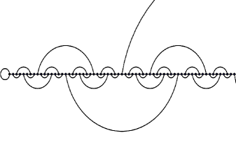
Figure 1: Depiction of the Hanoi network of generation $g=6$. The network features a regular geometric structure, in the form of a one dimensional backbone, and a distinct set of recursive small-world links. The node degree is uniformly $3$.

The Hanoi networks (Boettcher et al., 2008, 2009; Boettcher and Brunson, 2011; Boettcher and Li, 2015) are based on a simple geometric backbone, a one-dimensional line of $n=2^{g}$ nodes. Each node is at least connected to its nearest neighbor left and right on the backbone. To construct the hierarchy to $g$-th generation, consider parameterizing any node $x<n$ (except for zero) uniquely in terms of two integers $(i,j)$, $i\geq 1$ and $1\leq j\leq 2^{g-i}$, via

$$x = 2^{i-1}\left(2j-1\right).$$ (1)

Here, $i$ denotes the level of hierarchy whereas $j$ labels consecutive nodes within each hierarchy. Such a parametrization raises a natural pattern for long-range small-world edges that are formed by the neighbors $x=2^{i-1}(4j-3)$ and $y=2^{i-1}(4j-1)$ for $1\leq j\leq 2^{g-i-1}$, as shown in Fig.(1). Eventually, this procedure constructs a finite dimensional hierarchical network with a uniform finite node degree $3$, and a diameter of $\sim\sqrt{n}$, which is denoted as HN3 (Boettcher et al., 2008, 2009; Boettcher and Brunson, 2011).

To model the modular property of real-world brain networks, we replace each single node $x$ in HN3 by a fully-connected clique that contains a finite number $m$ of nodes, thus forming a network with size $n\times m$. Maintaining the structural properties of HN3, the self-similar structure, and the small-world connections, we design two connectivity patterns between moduli in the same hierarchy. In the first paradigm, the single edge in the original HN3 is now formed by two randomly chosen inter-clique nodes, which we denote as HMN1. The second paradigm is inspired by previous hierarchical modular models (Moretti and Muñoz, 2013; Ódor et al., 2015). To distinguish it from HMN1, we denote it as HMN2. Previous models share a common feature, the exponential distribution of the inter-moduli connectivity probability. Moduli are connected in either a stochastic way with a level-dependent probability $p_{i}$ or a deterministic way with a level-dependent number of edges.

Since an infinite dimensional network is predicted not to support the Griffiths phase (Moretti and Muñoz, 2013), to maintain a finite fractal dimension, the size of moduli exponentially increases as the inter-moduli connectivity probability exponentially decreases. Here, we use the stochastic scheme to construct HMN2. In HMN2, for the second hierarchy, the clique $2(2j-1)$ is grouped with the neighbor clique $2(2j-1)-1$ and $2(2j-1)+1$ forming a moduli. For the third hierarchy, the clique $2^{2}(2j-1)$ is grouped with three left neighbor cliques up to the clique $2^{2}(2j-1)-3$ and three right neighbor cliques up to the clique $2^{2}(2j-1)+3$. Repeating this procedure to $g$-th generation, the size of moduli of $i$-th generation is $m(2^{i}-1)$. The number of all possible stochastic connections between two moduli is $m^{2}\left(4^{i}-2^{i+1}+1\right)$. Thus, to ensure at least one edge between them, the level-dependent probability $p_{i}$ is at least $1/\left(m^{2}\left(4^{i}-2^{i+1}+1\right)\right)$.

III Susceptible-Infected-Susceptible Model and the Spectral Analysis

Certain fundamental dynamical models, the Susceptible-Infected-Susceptible (SIS) model and the Contact Process (CP), have been used to model the activity propagation on brain networks (Moretti and Muñoz, 2013; Ódor et al., 2015). Previous studies focus on the emergence of the Griffiths phase on general complex networks using these simplified models. Quenched disorder, either intrinsic to nodes or topological, has been shown to smear the phase transition at critical points and generate the Griffiths phase. Special $\mathcal{\mathsf{\mathit{rare}}}$ $\mathit{regions}$ (RRs) emerge in this dynamical process evolving on networks with quenched disorder. Statistically, the active state lingers in these rare regions for a typical time that grows exponentially with their sizes, and eventually ends up in the absorbing state (Griffiths, 1969; Noest, 1986; Vojta, 2006). The emerging exponentially distributed rare regions induce power-law decays with continuously varying exponents, i.e. the Griffiths phase.

The essential disorder can stem from a node-dependent propagation rate (intrinsic quenched disorder) (Muñoz et al., 2010; Juhász et al., 2012). Recent results also present evidence that the Griffiths phase emerges due to the quenched disorder on the edges, such as in tree networks with a correlated weight pattern (Odor and Pastor-Satorras, 2012) and in random networks with exponentially suppressed weight scheme (Ódor, 2013). The Quenched Mean-Field (QMF) approximation applies a spectral analysis on the network adjacency matrix that analytically explains emerging rare regions and the Griffiths phase on networks with the quenched disorder (Goltsev et al., 2012; Ódor, 2013). In absence of the quenched disorder, the Griffiths phase can also be a consequence of the structural heterogeneity of finite dimensional networks that is expected to have a similar role as the quenched disorder (Muñoz et al., 2010; Moretti and Muñoz, 2013). This analytical procedure successfully confirms the Griffiths phase on finite dimensional hierarchical modular networks in previous work (Moretti and Muñoz, 2013). In this section, we will focus on the SIS model and apply the spectral analysis on all the finite dimensional structures we consider.

III.1 SIS Model and the Simulation

In SIS model, each node in networks is described by a binary state, active ($\sigma=1$) or inactive ($\sigma=0$). An active node is deactivated with a unit rate, while it propagates the activity to its neighbors with a rate $\lambda$. The evolution equation for the probability $\rho_{x}\left(t\right)$ that node $x$ is active at time $t$ is

$$\frac{d}{dt}\rho_{x}\left(t\right) = -\rho_{x}\left(t\right)+\lambda\left[1-\rho_{x}\left(t\right)\right]\sum_{y=1}^{N}A_{xy}\rho_{y}\left(t\right),$$ (2)

in which $A_{xy}$ is the network adjacency matrix.

We here briefly introduce the method we use to perform the simulation for the SIS model. The large-scale numerical simulation method of the SIS model developed in (Ferreira et al., 2012) determines the critical propagation rate $\lambda_{c}$ efficiently for various networks. This algorithm considers the SIS model in continuous time. At each time step, one randomly chosen active node deactives with the probability $N_{i}/\left(N_{i}+\lambda N_{n}\right)$ where $N_{i}$ is the number of active nodes at time $t$, $N_{n}$ is the number of edges emanating from them. With complementary probability $\lambda N_{n}/\left(N_{i}+\lambda N_{n}\right)$, the active state is transmitted to one inactive neighbor of the randomly selected node. Time is incremented by $\triangle t=1/\left(N_{i}+\lambda N_{n}\right)$. This process is iterated after the system updating.

III.2 The Spectral Analysis for SIS Model

Here, we review the derivation of the criterion for the localization of steady active state on networks based on evaluation the inverse participation ratio (IPR) of eigenvectors of the adjacency matrix. Denote the eigenvalues and eigenvectors of the adjacency matrix $A_{xy}$ as $\Lambda_{i}$ and $f_{x}\left(\Lambda_{i}\right)$, for which $\Lambda_{1}\geq\Lambda_{2}\geq\cdots\geq\Lambda_{N}$. The probabilities $\rho_{x}$ at the steady state can be written as a linear superposition of the $N$ orthogonal eigenvectors (Goltsev et al., 2012),

$$\rho_{x} = \sum_{\Lambda}c\left(\Lambda\right)f_{x}\left(\Lambda\right).$$ (3)

If the largest eigenvalue $\Lambda_{1}$ is significantly larger than all the other eigenvalues, i.e., there is a spectral gap in the spectrum, then the QMF approximation predicts the critical point $\lambda_{c}$ to scale as $1/\Lambda_{1}$, and the steady state probability as

$$\rho_{x} \sim c\left(\Lambda_{1}\right)f_{x}\left(\Lambda_{1}\right).$$ (4)

At the critical $\lambda_{c}$, the order parameter $\rho$, defined as the average of active probability over all the nodes, can be expanded as,

$$\rho \sim a_{1}\triangle+a_{2}\triangle^{2}+\ldots,$$ (5)

in which $\triangle=\lambda\Lambda_{1}-1\ll 1$ with the coefficients

$$a_{i} = \frac{\sum_{x=1}^{N}f_{x}\left(\Lambda_{i}\right)}{N\sum_{x=1}^{N}f_{x}^{3}\left(\Lambda_{i}\right)}.$$ (6)

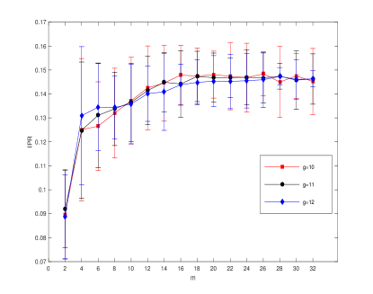
(a)

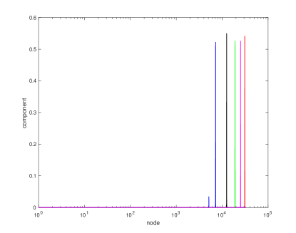
(b)

Figure 2: (a) IPR vs $m$ for HMN1 of different generation $g$. The red squares are IPRs for different $m$ with $g=10$; the black circles are IPRs with $g=11$; the blue diamonds are IPRs with $g=12$. Each data point averages IPRs over 100 independent realizations of HMN1. (b) the localized eigenvectors corresponding to five largest eigenvalues of the adjacency matrix of one graph realization of HMN1 for $g=11,m=16$.

With the dominant largest eigenvalue and the principle eigenvector, the order parameter $\rho$ can be approximated with $\rho\sim a_{1}\triangle$. In the limit $N\rightarrow\infty$, if the principle eigenvector $f_{x}\left(\Lambda_{1}\right)$ is localized, $a_{1}\sim O(1/N)$ and $\rho\sim O(1/N)$. Thus, the active state is localized on the a few nodes of the network. In turn, if the eigenvector $f_{x}\left(\Lambda_{1}\right)$ is delocalized $(\sim\sqrt{N})$, $a_{1}\sim const$ and $\rho\sim const$. Then, the active state extends over a finite fraction of nodes of the network. As proposed in (Goltsev et al., 2012), the localization of the principle eigenvector is quantified by the inverse participation ratio (IPR) of the principle eigenvector,

$$IPR\left(\Lambda\right) = \sum_{x=1}^{N}f_{x}^{4}\left(\Lambda\right).$$ (7)

A finite IPR corresponds to a localized principle eigenvector, while a IPR approaching to zero corresponds to a delocalized principle eigenvector. We apply the concept of IPR on all the networks we propose to examine whether a localized principle eigenvector exists, which in the QMF approximation may suggest the the emergence of rare regions and the Griffiths phase (Moretti and Muñoz, 2013; Ódor et al., 2015).

We analyze the principle eigenvector of the adjacency matrix of HMN1 for different generation $g$ with different size of basic cliques $m$. As shown in Fig.(2a), the IPR increases with $m$ towards to a finite value. Each single value of IPR in Fig.(2a) is derived by averaging over $100$ graph realizations of HMN1. Additionally, not only the largest eigenvalue, but actually a range of eigenvalues at the the higher edge in the spectrum have the localized eigenvectors, shown in Fig.(2b).

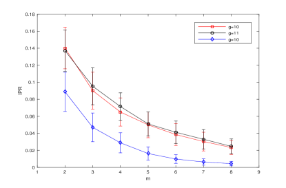
(a)

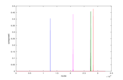
(b)

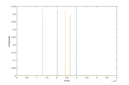
(c)

Figure 3: (a) IPR vs $m$ for HMN2 with different $g$. The red squares are values of the IPR with $g=10$; the black circles are IPRs for $g=11$. The level-dependent inter-moduli probability is $p_{i}=4^{-\left(i+1\right)}$. Compared to them, the bottom line with blue diamonds is for $g=10$ with a level-dependent probability $p_{i}=4^{-i}$. Each data point averages IPRs over 100 independent realizations of HMN2. (b): localized eigenvectors corresponding to five largest eigenvalues of the adjacency matrix of one graph realization of HMN2 with $g=14,m=2,p_{i}=4^{-\left(i+1\right)}$; (c): localized eigenvectors corresponding to five largest eigenvalues of the adjacency matrix of one graph realization of HMN2 with $g=14,m=3,p_{i}=4^{-\left(i+1\right)}$.

For HMN2, we work on simple level-dependent inter-moduli connectivity probabilities, $p_{i}=4^{-\left(i+1\right)}$ and $p_{i}=4^{-i}$. The backbone as well as the first hierarchy inter-moduli connectivity probability is fixed at $1/4$, where the moduli are the basic cliques described in Sec.II. The IPRs are shown in Fig.(3a), from which we find the largest IPR is from the the scheme that the single clique contains $2$ nodes, and the probability is $p_{i}=4^{-\left(i+1\right)}$. In this case, the network is statistically almost fragmented. Our numerical results in Sec.IV indeed show the emergence of the Griffiths phase as a trivial consequence of the network disconectedness. To obtain a connected network with a finite fractal dimension, we also perform the simulation of the case in which $m=3$ and $p_{i}=4^{-\left(i+1\right)}$. For HMN2, which is stochastically constructed, as the clique size $m$ or level-dependent probability increases, the inter-moduli connections become more and more dense and the IPR decreases, shown in Fig.(3a). The regime over the parameter $m$ or the level-dependent $p_{i}$ for the possible emergence of the Griffiths phase is narrow. However, the localized principle eigenvector exists for HMN2 with a finite IPR. In Fig.(3b) and Fig.(3c), we illustrate this result using two example graphs.

IV Simulation Results for the SIS Model on HMN1 and HMN2

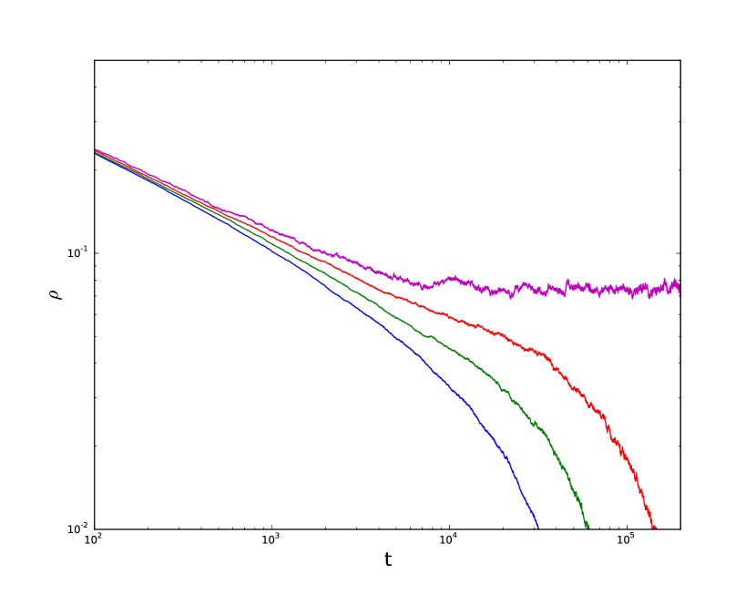
(a)

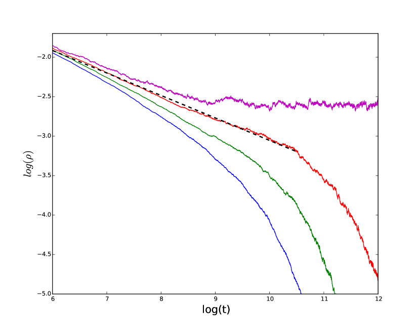
(b)

Figure 4: (a): $\rho$ vs $t$ for HMN1 with $g=11,m=8$; blue line: $\lambda=0.1650$; green line: $\lambda=0.1651$; red line: $\lambda=0.1652$; magenta line: $\lambda=0.1653$; (b): $\log\left(\rho\right)$ versus $\log\left(t\right)$ , the black dashed line is the fitted curve with $\rho\sim t^{-0.2849\ldots}$. The critical propagation rate is $\lambda_{c}\approx 0.1652$

In this section, we use the simulation method introduced in Sec.III.1 to run the SIS model on HMN1 and HMN2. The network is initialized as a fully-active graph. The system is updated each step until $t_{max}\left(10^{6}\right)$ is reached or in case of activity extinction. Simulations for each propagation rate $\lambda$ are repeated for $1000\sim 5000$ independent network realizations that are averaged over to obtain the order parameter $\rho\left(t\right)$. We also derive the effective decay exponent by fitting critical power laws $\rho\left(t\right)\sim t^{-\alpha_{eff}}$ with ((Ódor, 2013; Ódor et al., 2015))

$$\alpha_{eff} =-\frac{\ln\left[\rho\left(t\right)/\rho\left(t^{\prime}\right)\right]}{\ln\left(t/t^{\prime}\right)}$$ (8)

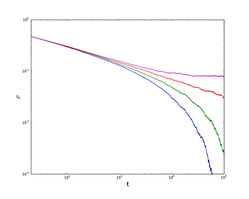
(a)

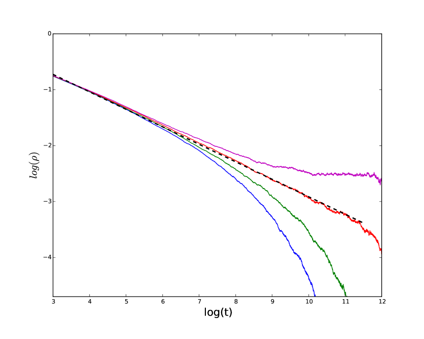
(b)

Figure 5: (a): $\rho$ vs $t$ for HMN1 with $g=11,m=16$; blue line: $\lambda=0.07475$; green line: $\lambda=0.0.07480$; red line: $\lambda=0.07485$; magenta line: $\lambda=0.0749$; (b): $\log\left(\rho\right)$ versus $\log\left(t\right)$ , the black dashed line is the fitted curve with $\rho\sim t^{-0.3127\ldots}$. The critical propagation rate is $\lambda_{c}\approx 0.07485$.

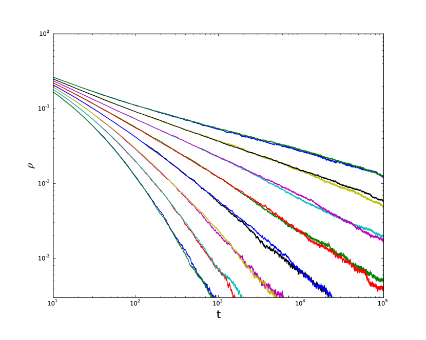
(a)

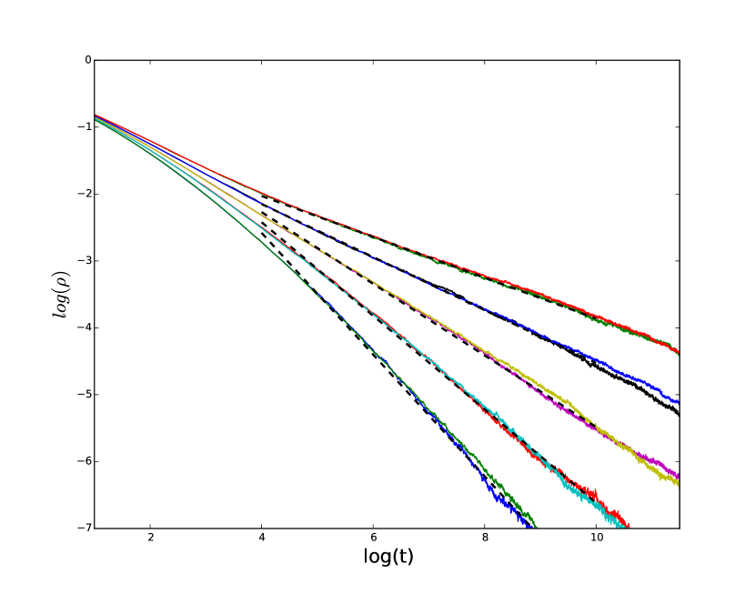
(b)

Figure 6: (a): $\rho$ vs $t$ for HMN2 with $g=13,m=2$ and with $g=14,m=2$. Lines from bottom to top are for $\lambda=0.46,0.47,0.48,0.49,0.50,0.51,0.52,0.53$. (b): $\log\left(\rho\right)$ versus $\log\left(t\right)$, the black dashed lines are the fitted curves with $\rho\sim t^{-0.9094\ldots}$, $\rho\sim t^{-0.6989\ldots}$, $\rho\sim t^{-0.5356\ldots}$, $\rho\sim t^{-0.3962\ldots}$ and $\rho\sim t^{-0.3054\ldots}$ from bottom to top for $\lambda=0.49,0.50,0.51,0.52,0.53$

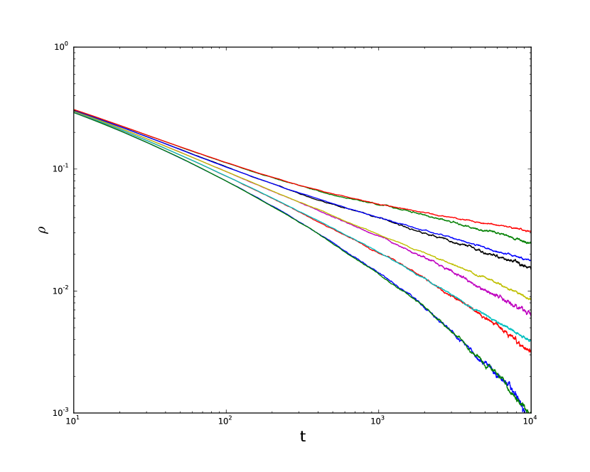
(a)

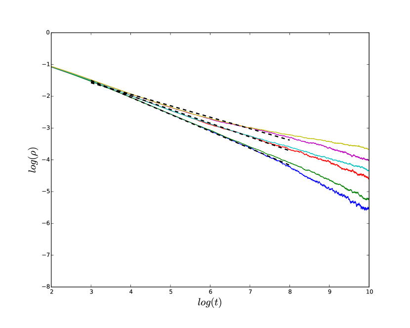
(b)

Figure 7: (a): $\rho$ vs $t$ for HMN2 with $g=13,m=3$ and with $g=12,m=3$. Lines from bottom to top are for propagation rates $\lambda=0.258,0.259,0.260,0.261,0.262$. (b): $\log\left(\rho\right)$ versus $\log\left(t\right)$, the black dashed lines from bottom to top are the fitted curves with $\rho\sim t^{-0.5339\ldots}$, $\rho\sim t^{-0.4325\ldots}$, $\rho\sim t^{-0.3605\ldots}$ for $\lambda=0.260,0.261,0.262$

In Fig.(4) and Fig.(5), we present the simulation results of the SIS model on HMN1 with $g=11,m=8$ and $g=11,m=16$, and fit with the effective decay exponent at the critical point. The Griffiths phase is absent in in HMN1, and we find trivial phase transition at criticality.

For HMN2 with $m=2$, the size-independent Griffiths phase emerges, shown in Fig.(6). However, the Griffiths phase is a trivial consequence of the disconnectedness of HMN2 when $p_{i}=4^{-\left(i+1\right)}$. We perform the simulation for HMN2 with $m=3,p_{i}=4^{-\left(i+1\right)}$ that is statistically almost certain to be connected. As the connections are established stochastically, there is a chance that all the possible inter-moduli edges fails to be connected. To avoid this case, we enforce at least one inter-moduli connection to exist by repeating the construction process in the simulation. The numerical results for a connected HMN2 is presented in Fig.(7). We find a nearly size-independent power laws in a stretched regime of $\lambda$. Comparing Fig.(6) with Fig.(7), we expect that, as $m$ increases while keeping $p_{i}$ fixed and $\mathcal{\mathsf{\mathit{vice}}}$ $\mathit{versa}$, the regime in the parameter space of $\lambda$ for the Griffiths phase becomes narrow until it disappears when HMN2 becomes high-dimensional.

V Conclusion

In this work, we construct two classes of synthetic hierarchical modular networks that possess a self-similar structure and small-world long range connections, based on the hierarchical Hanoi networks (Boettcher and Li, 2015). We study the Griffiths phase by evolving the fundamental SIS model on the HMNs we design. As an further exploration into a Griffiths phase that is caused by the structural heterogeneity of networks, we compare numerical results for two classes of networks. The results suggest the essential role of the exponential distribution of the inter-moduli connectivity probability or, equivalently, the size of moduli on the emergence of a Griffiths phase. The first class of hierarchical networks, HMN1, are not able to support the Griffiths phase, although they satisfy the structural criteria, such as the finite fractal dimension, the modular structure, the hierarchical heterogeneity. The second class of hierarchical networks, HMN2, are constructed to possess a hierarchical pattern in the inter-moduli connectivity probability and size of moduli, which therefore require a delicate tuning to maintain a connected, finite dimensional network. This significant difference in the design of hierarchical pattern results in the emergence of the Griffiths phase.

As a complement to the computational efforts, the spectral analysis proposed in the Quenched Mean Field approximation suggests that a finite IPR of the principle eigenvector of the network adjacency matrix can be considered as an indicator of the localization of activity that may result in the emergence of rare regions and the Griffiths phase under certain circumstances. Although all the networks we consider prove to have a finite IPR and localized eigenvectors corresponding to the higher edge of the spectrum, only when the structural disorder of inter-moduli connections is sufficient, the Griffiths phase appears. As an extension to previous finite dimensional models that support the Griffiths phase with a localized principle eigenvector (Moretti and Muñoz, 2013; Ódor et al., 2015), we find a class of finite dimensional networks with a localized principle eigenvector on which the Griffiths phase is absent. This raises questions on a more generalized theoretical analysis that applies to all the networks considered previously and currently.

VI Acknowledgements

I would like to thank Prof. Stefan Boettcher for helpful discussions. This work is supported by the NSF through grant DMR-1207431 is gratefully acknowledged.

References

- Moretti and Muñoz (2013) P. Moretti and M. A. Muñoz, Nature communications 4 (2013).
- Ódor et al. (2015) G. Ódor, R. Dickman, and G. Ódor, Scientific reports 5 (2015).
- Nykter et al. (2008) M. Nykter, N. D. Price, M. Aldana, S. A. Ramsey, S. A. Kauffman, L. E. Hood, O. Yli-Harja, and I. Shmulevich, Proceedings of the National Academy of Sciences 105, 1897 (2008).
- Furusawa and Kaneko (2012) C. Furusawa and K. Kaneko, Phys. Rev. Lett. 108, 208103 (2012), URL http://link.aps.org/doi/10.1103/PhysRevLett.108.208103.
- Beggs and Plenz (2003) J. M. Beggs and D. Plenz, The Journal of neuroscience 23, 11167 (2003).
- Plenz and Thiagarajan (2007) D. Plenz and T. C. Thiagarajan, Trends in neurosciences 30, 101 (2007).
- Beggs (2008) J. M. Beggs, Philosophical Transactions of the Royal Society of London A: Mathematical, Physical and Engineering Sciences 366, 329 (2008).
- Kinouchi and Copelli (2006) O. Kinouchi and M. Copelli, Nature physics 2, 348 (2006).
- Legenstein and Maass (2007) R. Legenstein and W. Maass, Neural Networks 20, 323 (2007).
- Barbieri and Shimono (2012) R. Barbieri and M. Shimono, Networking of Psychophysics, Psychology and Neurophysiology p. 61 (2012).
- Rubinov et al. (2011) M. Rubinov, O. Sporns, J.-P. Thivierge, and M. Breakspear, PLoS Comput Biol 7, e1002038 (2011).
- Wang and Zhou (2012) S.-J. Wang and C. Zhou, New Journal of Physics 14, 023005 (2012).
- Sporns et al. (2004) O. Sporns, D. R. Chialvo, M. Kaiser, and C. C. Hilgetag, Trends in cognitive sciences 8, 418 (2004).
- Meunier et al. (2010) D. Meunier, R. Lambiotte, and E. T. Bullmore, Frontiers in neuroscience 4, 200 (2010).
- Kaiser (2011) M. Kaiser, Neuroimage 57, 892 (2011).
- Boettcher et al. (2009) S. Boettcher, J. L. Cook, and R. M. Ziff, Physical Review E 80, 041115 (2009).
- Berker et al. (2009) A. N. Berker, M. Hinczewski, and R. R. Netz, Physical Review E 80, 041118 (2009).
- Boettcher and Brunson (2011) S. Boettcher and C. T. Brunson, Phys. Rev. E 83, 021103 (2011).
- Boettcher et al. (2012) S. Boettcher, V. Singh, and R. M. Ziff, Nature communications 3, 787 (2012).
- Singh and Boettcher (2014) V. Singh and S. Boettcher, Physical Review E 90, 012117 (2014).
- Singh et al. (2014) V. Singh, C. T. Brunson, and S. Boettcher, Phys. Rev. E 90, 052119 (2014).
- Boettcher et al. (2008) S. Boettcher, B. Gonçalves, and H. Guclu, Journal of Physics A: Mathematical and Theoretical 41, 252001 (2008).
- Boettcher and Li (2015) S. Boettcher and S. Li, Journal of Physics A: Mathematical and Theoretical 48, 415001 (2015).
- Goltsev et al. (2012) A. V. Goltsev, S. N. Dorogovtsev, J. G. Oliveira, and J. F. F. Mendes, Phys. Rev. Lett. 109, 128702 (2012).
- Griffiths (1969) R. B. Griffiths, Physical Review Letters 23, 17 (1969).
- Noest (1986) A. J. Noest, Physical review letters 57, 90 (1986).
- Vojta (2006) T. Vojta, Journal of Physics A: Mathematical and General 39, R143 (2006).
- Muñoz et al. (2010) M. A. Muñoz, R. Juhász, C. Castellano, and G. Ódor, Physical review letters 105, 128701 (2010).
- Juhász et al. (2012) R. Juhász, G. Ódor, C. Castellano, and M. A. Muñoz, Physical Review E 85, 066125 (2012).
- Odor and Pastor-Satorras (2012) G. Odor and R. Pastor-Satorras, Physical Review E 86, 026117 (2012).
- Ódor (2013) G. Ódor, Physical Review E 88, 032109 (2013).
- Ferreira et al. (2012) S. C. Ferreira, C. Castellano, and R. Pastor-Satorras, Physical Review E 86, 041125 (2012).
- Cota et al. (2016) W. Cota, S. C. Ferreira, and G. Ódor, Phys. Rev. E 93, 032322 (2016).