Eternal non-Markovianity: from random unitary to Markov chain realisations

Abstract

The theoretical description of quantum dynamics in an intriguing way does not necessarily imply the underlying dynamics is indeed intriguing. Here we show how a known very interesting master equation with an always negative decay rate [eternal non-Markovianity (ENM)] arises from simple stochastic Schrödinger dynamics (random unitary dynamics). Equivalently, it may be seen as arising from a mixture of Markov (semi-group) open system dynamics. Both these approaches lead to a more general family of CPT maps, characterized by a point within a parameter triangle. Our results show how ENM quantum dynamics can be realised easily in the laboratory. Moreover, we find a quantum time-continuously measured (quantum trajectory) realisation of the dynamics of the ENM master equation based on unitary transformations and projective measurements in an extended Hilbert space, guided by a classical Markov process. Furthermore, a Gorini-Kossakowski-Sudarshan-Lindblad (GKSL) representation of the dynamics in an extended Hilbert space can be found, with a remarkable property: there is no dynamics in the ancilla state. Finally, analogous constructions for two qubits extend these results from non-CP-divisible to non-P-divisible dynamics.

Introduction

A realistic modelling of many quantum phenomena inevitably needs to take into account the interaction of our system of interest with environmental degrees of freedom. Thus, in order to describe the quantum system dynamics appropriately, one is often forced to deal with open quantum systems. A very relevant and well understood class of such open quantum system dynamics follows from a Markov master equation of GKSL form ^{2; 3}. Non-Markovian behaviour may arise from a structured environment or strong system-environment interaction ⁴. Non-Markovian systems are very challenging: in the often-employed projection operator formalism their dynamics involves memory kernels ^{5; 6}. Other approaches range from path integrals ^{7; 8}, over hierarchical equations of motion (HEOM) for the reduced density matrix ^{9; 10}, to hierarchies of stochastic pure states (HOPS) ^{11; 12}. Sometimes time-convolutionless master equations can be used ¹³. During the last few years, due to tremendous experimental progress in quantum technologies in many different areas and more and more refined measurement schemes, specific investigations of non-Markovian quantum dynamics, where GKSL is no longer applicable, have become possible ^{14; 15; 16; 17; 18; 19}. Recent experiments also demonstrate how to use non-Markovianity for entanglement preservation ²⁰ and for a quantum information protocol ²¹.

The theory of non-Markovian quantum dynamics is much less developed than the GKSL class and subject of tremendous research over the last decade and more. A very valid point of view would be to call any dynamics other than GKSL semigroup evolution “non-Markovian”. A more detailed analysis, however, reveals an astonishing variety of possible definitions of what constitutes non-Markovian dynamics ^{22; 23; 24}, and therefore a large number of definitions and measures of non-Markovianity have been proposed ^{25; 26; 27; 28; 29; 30; 31; 32; 33}. So far, most studies are based on the effective dynamics of the reduced density operator, other consider the full dynamics of system and environment ^{34; 35}.

As mentioned earlier, in some cases of interest, the open system dynamics may be written in terms of a time-local master equation involving time-dependent functions as prefactors with otherwise GKSL form. Then, for some periods of time negative decay rates may show up, which according to some measures indicates non-Markovian dynamics ^{36; 37}. Recently, a remarkable master equation for a qubit was presented involving an always negative decay rate of an otherwise GKSL-type-looking master equation. It was termed the master equation of eternal non-Markovianity (ENM master equation) ^{36; 38}.

We expect non-Markovian dynamics to be related to some form of memory-dependence arising from the dynamics of the environmental degrees of freedom. This is why non-Markovianity is associated to a "backflow of information" ^{26; 39; 40; 41} or to the occurrence of quantum memory ²⁴, or simply to a joint complex system-environment dynamics ⁴². In such cases, the measures detect non-Markovianity. In this contribution we want to emphasize, however, that the reverse need not be true: there are non-Markovian master equations (according to one of the definitions), whose physical realisation does not support any notion of such "memory effects". Instead, either there is no dynamical environment at all, the dynamics can be realised by a classical Markov process or, when embedded in a larger Hilbert space, there is no dynamics of the environmental state.

In this paper we derive the ENM master equation from an appropriate mixture of Markov dynamics in two (related) ways: one is based on random unitary evolution, the second approach uses a mixture of Markov GKSL maps. By highlighting the equivalence of all these dynamics on the reduced level, we show explicitly how ENM evolution of a qubit could be realised in a laboratory either with a white noise or with a classical jump process with time independent jump probabilities. Moreover, also the bipartite GKSL representation, for which the ancilla state is frozen, is possible. Nonetheless, we may choose to describe the dynamics in terms of a negative-rate time-local master equation, or, involving a non-trivial memory integral. These findings support the point of view that the interpretation of non-Markovianity is elusive and great care has to be taken when talking about memory effects based solely on a reduced (master equation) description.

Time-local master equations and negative decay rates

For any total Hamiltonian of system and environment and for any product initial state, the dynamics of an open quantum system can be expressed in terms of the dynamical map $\rho(t)=\Lambda_{t}[\rho(0)],$ with $\Lambda_{t}$ completely positive and trace preserving (CPT). If $\Lambda_{t}$ is an invertible map then one finds the corresponding time-local generator $\mathcal{L}_{t}=\dot{\Lambda}_{t}\Lambda_{t}^{-1}$ such that a time-local master equation $\dot{\rho}(t)=\mathcal{L}_{t}[\rho(t)]$ follows. Assuming the semi-group property $\Lambda_{t+s}=\Lambda_{t}\Lambda_{s}$, the generator takes the GKSL form ^{2; 3} ($\hbar=1$):

$$\dot{\rho}(t)=-i[H,\rho(t)]+\sum\limits_{i}\left(L_{i}\rho(t)L_{i}^{+}-\frac{1}{2}\{L^{+}_{i}L_{i},\rho(t)\}\right),$$ (1)

here written in a canonical form, where the $L_{i}$ are traceless orthonormal operators. By any definition, dynamics described by the semigroup master equation is Markovian.

Generalised Markovian dynamics appears when the master equation takes the quasi-GKSL-form ^{36; 43}

$$\dot{\rho}(t) =-i[H(t),\rho(t)]$$

$$+\sum\limits_{i}\gamma_{i}(t)\left(L_{i}(t)\rho(t)L_{i}^{+}(t)-\frac{1}{2}\{L^{+}_{i}(t)L_{i}(t),\rho(t)\}\right),$$ (2)

with decay rates $\gamma_{i}(t)\geq 0$, for all $i$. Equation (Time-local master equations and negative decay rates) defines a reasonable dynamics if applied to any state at any time and therefore defines a CP-divisible dynamical map $\Lambda_{t}$ ⁴⁴, i.e. the dynamical map $\Lambda_{t}$ satisfies the following property $\Lambda_{t}=\Lambda_{t,s}\Lambda_{s}$ and the family of maps (propagators) $\Lambda_{t,s}$ is CPT for any $t>s$. It seems natural to regard dynamical maps $\Lambda_{t}$ with master equations of type (Time-local master equations and negative decay rates) for which $\gamma_{i}(t)<0$ for some $i$ and some $t$ as candidates for non-Markovian quantum dynamics. In these cases, the dynamical map is no longer CP-divisible. Indeed, some authors ³⁶ propose to use the negativity of decoherence rates as a definition of non-Markovianity of the dynamics. This approach is based on the fact that the canonical form of the master equation, defined in analogy to the Markov case (so the time dependent Lindblad operators are traceless, normalized and mutually orthogonal), is unique. Consequently, to all CPT maps generated by a master equation of form (Time-local master equations and negative decay rates) one can uniquely assign a set of $\gamma_{i}(t)$.

Actually, one also considers $\Lambda_{t,s}$ which is not necessarily CP. If $\Lambda_{t,s}$ is positive for all $t>s$ then one calls the evolution P-divisible. Recently, this notion was refined in ref. ⁴⁵ as follows: the evolution is $k$-divisible if $\Lambda_{t,s}$ is $k$-positive. CP-divisibility is fully characterised by the corresponding time-local generator $\mathcal{L}_{t}$ – all local decoherence rates $\gamma_{i}(t)$ are always non-negative. P-divisibility is more difficult to characterise on the level of the generator. One has the following property: if $\Lambda_{t}$ is P-divisible, then

$$\frac{d}{dt}||\Lambda_{t}[X]||_{1}\leq 0,$$ (3)

for all Hermitian operators $X$, where $||\cdot||_{1}$ is a trace norm. Actually, when $\Lambda_{t}$ is invertible then (3) implies P-divisibility. This property is very close to the so-called BLP condition ²⁶ which says that $\Lambda_{t}$ defines Markovian evolution if

$$\frac{d}{dt}||\Lambda_{t}[\rho_{1}-\rho_{2}]||_{1}\leq 0,$$ (4)

for all initial states $\rho_{1}$ and $\rho_{2}$. It is clear that CP-divisibility implies P-divisibility and this implies the BLP condition of information loss (4).

The very insightful example of ^{46; 36}, used throughout this work, is the unital dynamics (i.e.: $\Lambda_{t}[\leavevmode\hbox{\small 1\kern-3.8pt\normalsize 1}]=\leavevmode\hbox{\small 1\kern-3.8pt\normalsize 1}$) of a single qubit determined from the master equation

$$\dot{\rho}(t)=\frac{1}{2}\sum\limits_{k=1}^{3}\gamma_{k}(t)(\sigma_{k}\rho(t)\sigma_{k}-\rho(t)),$$ (5)

where $\sigma_{k}$ are the Pauli spin operators.

Defining $\lambda_{i}(t)=e^{-\Gamma_{j}(t)-\Gamma_{k}(t)}$, where $\Gamma_{k}(t)=\int_{0}^{t}\gamma_{k}(u)du$, and $\{i,j,k\}$ run over the cyclic permutations of $\{1,2,3\}$, one has the following conditions which guarantee that the evolution $\Lambda_{t}$ is CPT:

$$\lambda_{i}(t)+\lambda_{j}(t)\leq 1+\lambda_{k}(t).$$ (6)

Clearly, the corresponding dynamical map is CP-divisible iff $\gamma_{k}(t)\geq 0$. Interestingly, the dynamical map is P-divisible iff the weaker conditions are satisfied ^{47; 48}

$$\gamma_{i}(t)+\gamma_{j}(t)\geq 0\ ,\ \ i\neq j,$$ (7)

given the validity of (6). Actually, in this case P-divisibility is equivalent to the BLP condition (4).
Using the geometric measure of non-Markovianity based on the volume of admissible states ³², our one qubit dynamics is classified as Markov, too, as for all times $\gamma_{1}(t)+\gamma_{2}(t)+\gamma_{3}(t)>0$ ⁴⁷ is satisfied.

An interesting example of the generator was proposed in ref. ³⁶ - the ENM master equation, with

$$\gamma_{1}(t)=\gamma_{2}(t)=1, \gamma_{3}(t)=-\tanh(t),$$ (8)

where one rate is always negative: $\gamma_{3}(t)<0$ for all $t>0$. One easily checks that (6) are satisfied and hence the dynamical map is CPT. Clearly, the corresponding dynamical map is not CP-divisible because of the negativity of $\gamma_{3}(t)$. Moreover, conditions (7) are also satisfied which implies that the map is P-divisible ^{47; 48}.

Is this evolution non-Markovian? Based on the concept of CP-divisibility it is clearly non-Markovian. However, it satisfies condition (4), hence it is Markovian according to BLP. In the following we want to argue that the meaning of non-Markovianity for non-CP-divisible maps like those generated by (Time-local master equations and negative decay rates) with an always negative rate (8) needs to be discussed carefully. In particular, it can be highly misleading here to relate the formal property of “non-Markovianity” according to one of its definitions to some notion of “complex system-environment dynamics” or “backflow of information” from environment to system as will be exemplified in this paper.

We show that there is a whole family of master equations of type (Time-local master equations and negative decay rates) with $\gamma_{i}(t)<0$, for some $i$ and times $t$ that i) turn out to arise from random unitary Schrödinger dynamics, ii) are mere mixtures of Markovian semi-group dynamics, iii) allow for a physical realisation based on a classical Markov process. With these observations in mind, it is obvious, that the ENM master equation (or its two-qubits extension, see the "From one to two qubits dynamics and breaking also P-divisibility" and the "Bipartite GKSL representation" sections) needs not be related to any information backflow from dynamical environment. The particular choice (8) turns out to be a special case of this more general family of evolutions.

Markov dephasing dynamics

To start with, consider simple dephasing dynamics of a qubit given by a master equation of GKSL type ⁴⁹

$$\dot{\rho}(t)=\sigma_{\alpha}\rho(t)\sigma_{\alpha}-\rho(t),$$ (9)

where $\sigma_{\alpha}=\vec{n}_{\alpha}\cdot\vec{\sigma}$ is the Pauli matrix of some direction $\vec{n}_{\alpha}$ ($|\vec{n}_{\alpha}|=1$). With $\sigma_{\alpha}|\pm_{\alpha}\rangle=\pm|\pm_{\alpha}\rangle$, Eq. (9) leaves the populations $\langle+_{\alpha}|\rho(t)|+_{\alpha}\rangle$ and $\langle-_{\alpha}|\rho(t)|-_{\alpha}\rangle$ constant, the coherences $\langle+_{\alpha}|\rho(t)|-_{\alpha}\rangle$, $\langle-_{\alpha}|\rho(t)|+_{\alpha}\rangle$, however, decay with a factor ${\rm e}^{-2t}$.

Since this CPT map is unital, the dynamics is of random unitary or random external field type ^{50; 51; 52; 53; 54}. In fact, a physical realisation of Eq. (9) for pure initial states is easily obtained from a fluctuating field $\xi(t)$ driving the unitary Schrödinger dynamics:

$$i\partial_{t}|\psi(t)\rangle=\xi(t)\sigma_{\alpha}|\psi(t)\rangle.$$ (10)

Indeed, if $\xi(t)$ represents Gaussian real white noise with $\langle\!\langle\xi(t)\rangle\!\rangle_{\xi}=0$ and $\langle\!\langle\xi(t)\xi(s)\rangle\!\rangle_{\xi}=\delta(t-s)$, the noise-averaged state $\rho(t)=\left\langle\!\langle|\psi(t)\rangle\langle\psi(t)|\right\rangle\!\rangle_{\xi}$ is a solution of (9) (see also Supplementary Information). With the unitary $U_{\xi}(t,0):={\rm e}^{-i\int\limits_{0}^{t}\xi(s)ds\sigma_{\alpha}}$ we find for an arbitrary initial condition:

$$\rho(t)=\langle\!\langle U_{\xi}(t,0)\rho(0)U^{+}_{\xi}(t,0)\rangle\!\rangle_{\xi}.$$ (11)

As shown in Supplemetary Information, the noise average can easily be performed analytically to give the solution of (9) in Kraus form

$$\rho(t)=\frac{1}{2}\left((1+e^{-2t})\rho(0)+(1-e^{-2t})\sigma_{\alpha}\rho(0)\sigma_{\alpha}\right).$$ (12)

Mixture of Markov dephasing dynamics

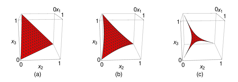
Figure 1: Inner region: set of parameters $(x_{1},x_{2},x_{3})$ with all three $\gamma_{k}(t)>0$ for some time t. (a) $t=0$ (defining triangle), (b) some later time $t>0$, (c) $t\rightarrow\infty$ (asymptotic area).

Now we allow the direction $\vec{n}_{\alpha}$ of the dephasing to be random with probability distribution $p(\vec{n}_{\alpha})$. From (12) we see that with $\vec{n}_{\alpha}=(n_{1}(\alpha),n_{2}(\alpha),n_{3}(\alpha))$, the averaged dynamics depends on the second order correlations

$$x_{kl}=\langle\!\langle n_{k}(\alpha)n_{l}(\alpha)\rangle\!\rangle_{\alpha}$$ (13)

only. Due to an overall orthogonal freedom of the whole problem, we may assume a diagonal $(x_{kl})$ and will from now on use the notation

$$x_{k}:=\langle\!\langle n_{k}^{2}(\alpha)\rangle\!\rangle_{\alpha},$$ (14)

assuming that $x_{kl}=0$ for $k\neq l$. As final result, the dynamical map arising from averaging over noise $\xi(t)$ and direction $\vec{n}_{\alpha}$ is again a map given in Kraus form by:

$$\rho(t) = \langle\!\langle U_{\xi}(t,0)\rho(0)U^{+}_{\xi}(t,0)\rangle\!\rangle_{\xi,\alpha}$$

$$= \frac{1}{2}(1+e^{-2t})\rho(0)+\frac{1}{2}(1-e^{-2t})\sum\limits_{k=1}^{3}x_{k}\sigma_{k}\rho(0)\sigma_{k}.$$

The three positive parameters $x_{1},x_{2},x_{3}$, with $x_{1}+x_{2}+x_{3}=1$ (the Cartesian variances of the distribution) are the only quantities of $p(\vec{n}_{\alpha})$ that determine the dynamics. In Bloch representation this corresponds to a monotonic and (in general) anisotropic shrinking of the Bloch sphere (see Supplementary Information).

Therefore, it also follows that (Mixture of Markov dephasing dynamics) can be obtained from a mixture of just three orthogonal dephasing directions along the Cartesian axes. Accordingly, the underlying dynamical map may be written as a mixture of three Markov (semigroup) dynamical maps according to

$$\Lambda_{t}=x_{1}e^{t\mathcal{L}_{1}}+x_{2}e^{t\mathcal{L}_{2}}+x_{3}e^{t\mathcal{L}_{3}}\ ,$$ (16)

where $\rho(t)=\Lambda_{t}[\rho(0)]$, $\mathcal{L}_{k}[\rho(t)]=\sigma_{k}\rho(t)\sigma_{k}-\rho(t)$ as in (9). The variances may thus be seen as probabilities $x_{k}$ of choosing either of three semigroup evolutions $e^{t\mathcal{L}_{k}}$ for the dynamics.

We conclude that dephasing dynamics in random directions can be written in two ways as a mixture of CP-divisible maps. Representation (Mixture of Markov dephasing dynamics) is a continuous mixture of unitary (Schrödinger) time evolutions, while in (16) we have a discrete, finite sum of irreversible Markov GKSL dynamics. As we will show next, the corresponding master equation is just (5), with possibly negative rates.

Master equation and negativity of decay rates. As shown in Supplementary Information, we find that the map $\Lambda_{t}$ from (16) satisfies the time-local master equation

$$\dot{\Lambda}_{t}=\mathcal{L}_{t}\Lambda_{t},$$ (17)

with the generator of the dynamics acting on density operators according to

$$\mathcal{L}_{t}[\rho(t)]=\frac{1}{2}\sum_{k=1}^{3}\gamma_{k}(t)(\sigma_{k}\rho(t)\sigma_{k}-\rho(t))\ ,$$ (18)

as in (5). The time dependent decoherence rates can be expressed as

$$\gamma_{1}(t) = \left(\mu_{1}(t)-\mu_{2}(t)-\mu_{3}(t)\right),$$

$$\gamma_{2}(t) = \left(-\mu_{1}(t)+\mu_{2}(t)-\mu_{3}(t)\right),$$ (19)

$$\gamma_{3}(t) = \left(-\mu_{1}(t)-\mu_{2}(t)+\mu_{3}(t)\right),$$

with

$$\mu_{1}(t)=-\frac{x_{2}+x_{3}}{x_{2}+x_{3}+e^{2t}x_{1}}, \mu_{2}(t)=-\frac{x_{3}+x_{1}}{x_{3}+x_{1}+e^{2t}x_{2}},$$

$$\mu_{3}(t)=-\frac{x_{1}+x_{2}}{x_{1}+x_{2}+e^{2t}x_{3}}\ .$$

As we will work out in detail, these rates need not be positive. Thus, the random mixture of Markovian dephasing leads to a time-local master equation with possibly negative decay rates.

Discussion of the negativity of the rates. The parameter set of variances (or probabilities) $x_{1},x_{2},x_{3}$ with $x_{1}+x_{2}+x_{3}=1$ and $x_{k}$ positive represents a triangular area in 3-dimensional space spanned by the vectors $\vec{r}=(x_{1},x_{2},x_{3})$, see Fig. 1. We refer to that set as the parameter triangle. We display in Fig. 1 (hatched) that subset of parameters, for which all $\gamma_{k}(t)$ are positive at that particular time t: (a) $t=0$, (b) some intermediate time $t>0$, and (c) $t\rightarrow\infty$. Clearly, initially for $t=0$, all $\gamma_{k}(0)=2x_{k}\geq 0$ are non-negative. Later, only a symmetric triangular-star shaped region near the centre reaching out to the tips of the parameter triangle corresponds to choices of parameters for which all $\gamma_{k}(t)$ are non-negative. Regions near the edges of the parameter triangle but away from the lines connecting the vertices with the centre of the triangle correspond to choices of the $x_{k}$ that lead to a negative $\gamma_{k}(t)$ for some $t>t_{*}$. As $t\rightarrow\infty$, an asymptotic finite area of that shape remains (we call it asymptotic area) for which all $\gamma_{k}(t)\geq 0$ for all times. We will investigate the shape and size of that area in more detail later.

The rates have the following seven properties: i) All rates start off non-negatively, $\gamma_{k}(0)=2x_{k}\geq 0$. ii) At most one $\gamma_{k}(t)$ can turn negative. iii) Once a $\gamma_{k}(t)$ turns negative at $t=t_{*}$, it remains negative ever after: $\gamma_{k}(t)<0$ for all $t>t_{*}$ (and the other two rates are always positive). iv) At the vertices of the defining triangle one of the $\gamma_{k}(t)$ equals $2$, the other two equal $0$ and all three remain at those constant values (GKSL). v) All $x_{1},x_{2},x_{3}$ lying on the edges of the triangle (except vertices), i.e. when exactly one of the $x_{k}=0$, give one of the $\gamma_{k}(t)<0$ for all $t>0$. The ENM master equation is of that kind with $x_{1}=x_{2}=\frac{1}{2}$ and $x_{3}=0$. In those cases the dephasing is complete in that direction, and the corresponding probability distribution has a form $p(\vec{n}_{\alpha})=p(n_{i},n_{j})\delta(n_{k}).$ vi) For all parameters outside the asymptotic parameter area there exists some time $t_{*}>0$, so that for all $t<t_{*}$ all $\gamma_{k}(t)$ are positive, and for all $t>t_{*}$ one of the $\gamma_{k}(t)$ is negative. vii) We have $\gamma_{1}(t)+\gamma_{2}(t)\geq 0$ for all times (and cyclic) and thus, the dynamics is P-divisible for all times and all choices of parameters ^{45; 47; 55}.

We thus see that (quasi-)GKSL dynamics is only realised for our dephasing in random directions-process for choices of $(x_{1},x_{2},x_{3})$ within the asymptotic parameter area. Outside that area one of the rates turns negative eventually (or immediately, for values at the border) and thus, the corresponding CPT map is not CP-divisible. Remarkably, for all possible choices of parameters, the map is P-divisible ⁴⁷.

If the possible parameters $(x_{1},x_{2},x_{3})$ are uniformly distributed over the parameter triangle, the probability for the corresponding dephasing process in random directions to be of quasi-GKSL type is just the area of the asymptotic area relative to the full parameter triangle.

As expanded in detail in Supplementary Information, in an appropriate parametrization, the shape of the asymptotic area is determined by one of Newton’s cubic curves ⁵⁶,

$$x^{2}y+x-y=0.$$ (20)

For the relative area of parameters outside the asymptotic (hatched) area, we find

$$\frac{A_{\rm{\text{non-CP-div}}}}{A_{\rm{\text{tot}}}}=\int\limits_{0}^{\sqrt{5}-2}dx\frac{6(3-3x-3x^{2}-x^{3})x}{\sqrt{1-\frac{4x}{1-x^{2}}}(1-x^{2})(1+x)}\approx 0.87,$$ (21)

see Supplementary Information. Interestingly, only $13\%$ of all dephasing in random directions dynamical maps are CP-divisible or of quasi-GKSL type. In particular, near the tips of the triangles, as the sides turn into tangents, only a vanishingly small set of CP-divisible maps remains for small fluctuations around a Cartesian direction. Thus, dephasing in one of the Cartesian directions with only the slightest fluctuations around that direction leads to a dynamics with negative dephasing rate with an overwhelming probability.

Memory kernel master equation

It is worth noting that the dynamics (Mixture of Markov dephasing dynamics) can also be described with a master equation involving a memory kernel ^{5; 6}

$$\dot{\rho}(t)=\int\limits_{0}^{t}K(t-s)\rho(s)ds.$$ (22)

For our dynamics, we find a kernel of the following form:

$$K(t-s)\rho(s)=\frac{1}{2}\sum_{k=1}^{3}K_{k}(t-s)(\sigma_{k}\rho(s)\sigma_{k}-\rho(s)),$$ (23)

with

$$K_{k}(t)=x_{k}\delta(t)+\eta_{k}(t)$$ (24)

and

$$\eta_{1}(t) = \frac{1}{2}\left(X_{1}(t)-X_{2}(t)-X_{3}(t)\right),$$

$$\eta_{2}(t) = \frac{1}{2}\left(-X_{1}(t)+X_{2}(t)-X_{3}(t)\right),$$

$$\eta_{3}(t) = \frac{1}{2}\left(-X_{1}(t)-X_{2}(t)+X_{3}(t)\right)\ ,$$ (25)

with $X_{k}(t)=x_{k}(1-x_{k})e^{-x_{k}t}$. Hence

$$K(t)= \frac{1}{2}\left(x_{1}\mathcal{L}_{1}+x_{2}\mathcal{L}_{2}+x_{3}\mathcal{L}_{3}\right)\delta(t)$$

$$+\frac{1}{2}\left(\eta_{1}(t)\mathcal{L}_{1}+\eta_{2}(t)\mathcal{L}_{2}+\eta_{3}(t)\mathcal{L}_{3}\right).$$

Interestingly, the memory kernel $K(t)$ has the following structure

$$K(t)=K_{\rm loc}\delta(t)+K_{\rm nloc}(t),$$ (26)

where the time-local part $K_{\rm loc}=\frac{1}{2}(x_{1}\mathcal{L}_{1}+x_{2}\mathcal{L}_{2}+x_{3}\mathcal{L}_{3})$ is just the weighted sum of the three Cartesian GKSL dephasing generators. The non-local part depends on three smooth functions $\eta_{k}(t)$.

As observed in ref. ⁵⁷ and confirmed here, a local in time master equation description of the dynamics has complementary properties to a memory kernel master equation, in the sense that a "nice" functional form in one formulation may lead to a more singular description in the other.

We see that the mixture of Markovian dephasing dynamics studied in this paper “ $x_{1}e^{t\mathcal{L}_{1}}+x_{2}e^{t\mathcal{L}_{2}}+x_{3}e^{t\mathcal{L}_{3}}$” may well be written in a form involving a “memory integral”, that is, apart from the more or less clear local term $K_{\rm loc}$ it contains a truly non-local part $K_{\rm nloc}(t)$. In open quantum system dynamics, non-local master equations of type (22) appear naturally from a dynamical environment, as, for instance, in the Nakajima-Zwanzig approach ^{5; 6}. Obviously, no dynamical environment exists in our constructions.

Classical Markov process representation of dynamics

So far we have acknowledged that the simple mixture of Markovian dynamics may well lead to a master equation involving negative rates. Remarkably, as we will explain in this section, that latter master equation may easily be simulated using a classical Markov process.

We start with the Kraus representation of the dephasing dynamics in random directions, Eq. (Mixture of Markov dephasing dynamics). We introduce the unitarily transformed states $\rho_{k}:=\sigma_{k}\rho(0)\sigma_{k}$, $k=0,...,3$ (with $\sigma_{0}=\leavevmode\hbox{\small 1\kern-3.8pt\normalsize 1}$) and corresponding probabilities $p_{k}(t)$ such that the state at time $t$ reads $\rho(t)=\sum\limits_{k=0}^{3}p_{k}(t)\rho_{k}$. The probabilities

$$p_{0}(t)=\frac{1}{2}\left(1+{\rm e}^{-2t}\right), p_{k}(t)=\frac{x_{k}}{2}\left(1-{\rm e}^{-2t}\right)$$ (27)

can be read off from the Kraus representation (Mixture of Markov dephasing dynamics).

As elaborated upon in Supplementary Information, these probabilities are solutions of the rate equations

$$\frac{d}{dt}\left(\begin{array}[]{c}p_{0}(t)\\ p_{1}(t)\\ p_{2}(t)\\ p_{3}(t)\end{array}\right)=\left(\begin{array}[]{cccc}-1&1&1&1\\ x_{1}&-1&0&0\\ x_{2}&0&-1&0\\ x_{3}&0&0&-1\end{array}\right)\left(\begin{array}[]{c}p_{0}(t)\\ p_{1}(t)\\ p_{2}(t)\\ p_{3}(t)\end{array}\right)$$ (40)

that are of the form of a classical Pauli master equation ⁵⁸

$$\dot{p}_{k}(t)=\sum_{j}\Big{(}\Gamma_{j\rightarrow k}p_{j}(t)-\Gamma_{k\rightarrow j}p_{k}(t)\Big{)},$$ (41)

with positive an time-independent rates $\Gamma_{0\rightarrow k}=x_{k},\Gamma_{k\rightarrow 0}=1$, and all other rates being zero. The corresponding transitions are displayed in Fig. 2.

Most remarkably, despite the negativity of the rates of the underlying quantum master equation, its solution $\rho(t)$ can be obtained from the classical Markov master equation (41) according to the following construction. Take a classical process between four classical states $\{r_{0},r_{1},r_{2},r_{3}\}$ as determined from the classical master equation (41). For a transition from state $r_{0}$ to some $r_{k}$ (with $k=1,2,3$), apply the unitary transformation $\sigma_{k}$ to the state, so that $\rho_{0}\rightarrow\rho_{k}$ occurs with rate $\Gamma_{0\rightarrow k}=x_{k}$. Equally, if a jump from $r_{k}$ ($k=1,2,3$) back to $r_{0}$ occurs, again apply the unitary $\sigma_{k}$ to the current state so that $\rho_{k}\rightarrow\rho_{0}$ with rate $\Gamma_{k\rightarrow 0}=1$. No other jumps can take place, see Fig. 2.

Figure 2: Graphical representation of a master equation (40) with $\rho_{j}=\sigma_{j}\rho\sigma_{j}$, with $\sigma_{0}=\leavevmode\hbox{\small 1\kern-3.8pt\normalsize 1}$, where jumps $\rho_{0}\rightarrow\rho_{1}$ occur with rate $\Gamma_{01}$ ($=x_{1}$), and $\rho_{1}\rightarrow\rho_{0}$ with rate $\Gamma_{10}$ ($=1$) , etc. No jumps $\rho_{1}\rightarrow\rho_{2}$, $\rho_{2}\rightarrow\rho_{1}$ nor $\rho_{1}\rightarrow\rho_{3}$,…, take place.

By construction, $\rho(t)=\sum\limits_{k=0}^{3}p_{k}(t)\rho_{k}$ is the solution (Mixture of Markov dephasing dynamics). Consequently, one can also simply generate the probability distribution $p_{k}(t)$ simulating the classical Markov process and afterwards accordingly mix the final density matrix using the four $\rho_{k}$.

We have managed to describe the process (5) based on the classical master equation (41) with positive, time independent rates. So we find a Markov chain representation of ENM.

Negative rate classical master equation. Starting from the time-local master equation (5) and writing its solution in the form of the dynamical map

$$\Lambda_{t}[\rho(0)]=\sum_{j=0}^{3}P_{j}(t)\sigma_{j}\rho(0)\sigma_{j},$$ (42)

we obtain the following equation for the probability 4-vector $\vec{P}(t)$ (for clarity we suppress the time dependence of $\gamma_{j}(t)$):

$$\frac{d}{dt}\left(\begin{array}[]{c}P_{0}(t)\\ P_{1}(t)\\ P_{2}(t)\\ P_{3}(t)\end{array}\right) =\frac{1}{2}\left(\begin{array}[]{cccc}-\gamma_{0}&\gamma_{1}&\gamma_{2}&\gamma_{3}\\ \gamma_{1}&-\gamma_{0}&\gamma_{3}&\gamma_{2}\\ \gamma_{2}&\gamma_{3}&-\gamma_{0}&\gamma_{1}\\ \gamma_{3}&\gamma_{2}&\gamma_{1}&-\gamma_{0}\end{array}\right)\left(\begin{array}[]{c}P_{0}(t)\\ P_{1}(t)\\ P_{2}(t)\\ P_{3}(t)\end{array}\right),$$ (55)

where $\gamma_{0}(t):=\gamma_{1}(t)+\gamma_{2}(t)+\gamma_{3}(t)$. It can be rewritten in the form of a Pauli master equation

$$\dot{P}_{k}(t)=\frac{1}{2}\sum\limits_{j}\left(\gamma_{j\rightarrow k}(t)P_{j}(t)-\gamma_{k\rightarrow j}(t)P_{k}(t)\right),$$ (56)

with $\gamma_{0\rightarrow j}(t)=\gamma_{j\rightarrow 0}(t)=\gamma_{j}(t)$, $\gamma_{k\rightarrow j}(t)=\gamma_{l}(t)$, for $k\neq j\neq l$ ($k,j,l=1,2,3$). As for the quantum master equation the transition rates can turn negative, equation (56) does not define a proper Markov process.

The solution

$$\vec{P}(t)=T(t)\vec{P}(0)$$

can be obtained from the propagator $T(t)$ as given in Supplementary Information. For the initial condition $\vec{P}(0)=(1,0,0,0)^{T}$ we find positive $P_{k}(t)$ for all $t$. Thus, despite the negative rates, the master equation (56) defines a proper evolution for a probability distribution for that particular choice of $\vec{P}(0)$. Similarly, for that initial condition only, we have $\Lambda_{0}=\leavevmode\hbox{\small 1\kern-3.8pt\normalsize 1}$.
Due to the negative rates one is tempted to think of (56) as representing a non-Markovian jump process. Yet, it is clear that $\vec{P}(t)=\vec{p}(t)$ for initial condition $(1,0,0,0)^{T}$, and $\vec{P}(t)$ is therefore also a solution of a Markovian jump process (41). Hence, one should also be careful with the interpretation of classical master equations involving negative rates.

Special case. For the special choice of $\gamma_{k}(t)$ given in Eq. (8) (introduced in ref. ³⁶) and assuming $P_{0}(0)=1$ and $P_{k}(0)=0$ one finds

$$P_{0}(t) = \frac{1}{2}(1+e^{-2t})$$ (57)

$$P_{1}(t) = P_{2}(t)=\frac{1}{4}(1-e^{-2t})$$ (58)

$$P_{3}(t) = 0\ .$$ (59)

Hence $P_{3}(t)$ is irrelevant and the solution is generated from (40) via the simplified Markov chain:

$$\frac{d}{dt}\left(\begin{array}[]{c}P_{0}(t)\\ P_{1}(t)\\ P_{2}(t)\end{array}\right)=\left(\begin{array}[]{ccc}-2&2&2\\ 1&-2&0\\ 1&0&-2\end{array}\right)\left(\begin{array}[]{c}P_{0}(t)\\ P_{1}(t)\\ P_{2}(t)\end{array}\right),$$ (60)

with positive $\gamma_{1}=\gamma_{2}=1$. It is evident that (60) generates a Markov semigroup. For a discussion for different initial conditions see Supplementary Information.

Realisation with orthogonal states. Note that the $\rho_{j}=\sigma_{j}\rho(0)\sigma_{j}$ are not mutually orthogonal, so they cannot be distinguished faithfully by a measurement. However, a truly classical implementation involving four classical (i.e. orthogonal) states can be found by expanding the dimension of our system to four qubits ($H=H^{A}\otimes H^{B}=\mathbb{C}^{2}\otimes\mathbb{C}^{8}$).

For this construction, we define the following extended dynamics involving the three ancilla qubits:

$$\dot{\tilde{\rho}}(t)=\frac{1}{2}\sum\limits_{k=1}^{3}\gamma_{k}(t)((\sigma_{k}\otimes U_{k})\tilde{\rho}(t)(\sigma_{k}\otimes U^{+}_{k})-\tilde{\rho}(t)),$$ (61)

where $U_{k}$ are unitary operators, specified below.
Tracing out the ancilla (B) degrees of freedom, this dynamics reduces to (5).

To construct the four orthonormal states we write the initial density operator in diagonal form:

$$\rho_{0}=p_{1}|\phi_{1}\rangle\langle\phi_{1}|+p_{2}|\phi_{2}\rangle\langle\phi_{2}|,$$

with orthonormal vectors $|\phi_{1}\rangle,|\phi_{2}\rangle$ and non-negative probabilities $p_{1},p_{2}=1-p_{1}$. Our four-qubit states are defined in the following way:

$$|\Psi_{0}\rangle =\sqrt{p_{1}}|\phi_{1}\rangle|\psi_{1}\rangle+\sqrt{p_{2}}|\phi_{2}\rangle|\psi_{2}\rangle,$$

$$|\Psi_{k}\rangle =\sqrt{p_{1}}\sigma_{k}\otimes U_{k}|\phi_{1}\rangle|\psi_{1}\rangle+\sqrt{p_{2}}\sigma_{k}\otimes U_{k}|\phi_{2}\rangle|\psi_{2}\rangle,$$

where the $U_{k}$ are chosen, such that $U_{k}|\psi_{i}\rangle=|\psi_{2k+i}\rangle$ and $|\psi_{l}\rangle\in\mathbb{C}^{8}$, $l=1,...,8$ are mutually orthogonal and normalized.

These four vectors of course don’t build a basis of the $\mathbb{C}^{16}$. Nonetheless, if we set $|\Psi_{0}\rangle\langle\Psi_{0}|$ as the initial state of our four-qubit system and let it evolve according to (61), the output state is always a mixture of these four states.

Consequently, we get a realisation of the dynamics (5) with distinguishable states. In a lab, therefore, one might choose to measure in a time-continuous fashion the actual four-qubit state such as to have a time-continuous (Markov) realisation of the classical process described in Fig. 2. By construction, the ensemble mean of the corresponding reduced states, at all times of continuous monitoring, is a solution of the original negative-rate master equation.

From one to two qubits dynamics and breaking also P-divisibility. From the non-CP-divisibility of the one qubit dynamical map (16) one can conclude that the corresponding map for two qubits, where the first qubit undergoes the dynamics (16) and the second one is frozen, is not P-divisible. Nonetheless, also in this case we can find a classic Markov process representation, which can be realised with orthogonal states.
To show this we expand the initial state of the two-qubit system in a following form:

$$\rho_{AB}(0)=\sum\limits_{ikmn=1}^{2}a_{ikmn}|\varphi_{i}\rangle\langle\varphi_{k}|\otimes|\psi_{m}\rangle\langle\psi_{n}|,$$ (62)

where $|\varphi_{1}\rangle$, $|\varphi_{2}\rangle$ are the eigenstates of the first qubit $A$ (with the corresponding eigenvalues $p_{1}$, $p_{2}$, $p_{1}+p_{2}=1$) and $|\psi_{1}\rangle$, $|\psi_{2}\rangle$ are two orthogonal states of the second qubit $B$. Equation (62) represents a general initial state, also entangled states are included.
The coefficients $a_{ikmn}$ are some complex numbers, which have to satisfy

$$\rho_{A}(0)=Tr_{B}(\rho_{AB}(0))=p_{1}|\varphi_{1}\rangle\langle\varphi_{1}|+p_{2}|\varphi_{2}\rangle\langle\varphi_{2}| \Leftrightarrow$$

$$\sum\limits_{l=1}^{2}a_{11ll}=p_{1}, \sum\limits_{l=1}^{2}a_{22ll}=p_{2}, \sum\limits_{l=1}^{2}a_{12ll}=\sum\limits_{l=1}^{2}a_{21ll}=0,$$ (63)

$$\rho_{AB}(0)=\rho^{+}_{AB}(0) \Leftrightarrow a_{ikmn}=a^{*}_{kinm}.$$ (64)

For the initial jump state in the extended Hilbert space (by a third system $C$) we make an ansatz:

$$|\xi_{0}\rangle=\sum\limits_{ik=1}^{2}\sum\limits_{l=1}^{4}c_{ikl}|\varphi_{i}\rangle|\psi_{k}\rangle|\chi_{l}\rangle,$$

where $|\chi_{l}\rangle$ are mutually orthogonal. The 16 coefficients $a_{ikmn}$ are mapped on the 16 coefficients $c_{ikl}$ with $a_{ikmn}=\sum\limits_{l=1}^{4}c_{iml}c^{*}_{knl}$, following from $\rho_{AB}(0)=Tr_{C}(\rho_{0})=Tr_{C}(|\xi_{0}\rangle\langle\xi_{0}|)$.
Per construction, Eq. (64) is fulfilled, also the positivity of the $p_{1}$, $p_{2}$ is guaranteed for all $c_{ikl}$. The other conditions for $a_{ikmn}$ put some constraints on the possible choice of $c_{ikl}$.
The other jump states take the form ($j=1,2,3$):

$$|\xi_{j}\rangle=\sum\limits_{ik=1}^{2}\sum\limits_{l=1}^{4}c_{ikl}(\sigma_{j}\otimes\leavevmode\hbox{\small 1\kern-3.8pt\normalsize 1}\otimes V_{j})|\varphi_{i}\rangle|\psi_{k}\rangle|\chi_{l}\rangle,$$

where the unitary $V_{j}$ are chosen, such that $V_{j}|\chi_{l}\rangle=|\chi_{4j+l}\rangle$ and $|\chi_{i}\rangle\in\mathbb{C}^{16}$, $i=1,...,16$ are mutually orthogonal and normalized. Consequently, $|\xi_{0}\rangle,...,|\xi_{3}\rangle$ are mutually orthogonal. To achieve this we have to extend our Hilbert space by four qubits, so overall our system consists of six qubits.
Fulfilment of condition (63) guarantees that $Tr_{B,C}(\rho_{j})=Tr_{B,C}(|\xi_{j}\rangle\langle\xi_{j}|)=\sigma_{j}\rho_{A}(0)\sigma_{j}$. In addition, the state of the second B qubit is the same for all $|\xi_{0}\rangle,...,|\xi_{3}\rangle$.
Accordingly, also the dynamics of two qubits, where the first undergoes (16) and the second is frozen, can be mapped on the (time-continuous limit of the) Markov jump process graphically represented in Figure 2, where the states $\rho_{k}$ are redefined. From this we conclude, that there are non-P-divisible maps, for which a classical Markov process description is possible. Therefore, both non-CP-divisibility ⁴⁷, but also the weaker non-P-divisibility ³⁹, are questionable indicators for the occurrence of memory effects associated with dynamics of environmental degrees of freedom.

Bipartite GKSL representation. Interestingly, the dynamics defined by (Mixture of Markov dephasing dynamics) may be represented via

$$\Lambda_{t}[\rho(0)]=\operatorname{Tr}_{E}({\rm e}^{t\mathcal{L}}[\rho(0)\otimes\rho_{E}]),$$ (65)

where $\mathcal{L}$ denotes a time independent bipartite GKSL generator. This construction is based on the correlated projection method ^{59; 60}: one defines the initial state of the bipartite system to be the following quantum-classical state

$$\tilde{\rho}(0)=\sum_{i=1}^{3}\rho_{i}(0)\otimes|i\rangle\langle i|,$$ (66)

where $|i\rangle$ are orthonormal vectors in $\mathcal{H}_{E}=\mathbb{C}^{3}$. Suppose now that the generator $\mathcal{L}$ gives rise to $e^{t\mathcal{L}}\tilde{\rho}(0)=\sum_{i=1}^{3}\rho_{i}(t)\otimes|i\rangle\langle i|$, that is, the bipartite evolution preserves the structure (66). Then the partial trace $\rho(t)=\operatorname{Tr}_{E}\tilde{\rho}(t)$ is defined by $\rho(t)=\sum_{i}\rho_{i}(t)$. Note that in general this prescription does not define a dynamical map ⁵⁹. However, if $\rho_{i}(0)=x_{i}\rho(0)$, then (66) defines a product state $\rho(0)\otimes\rho_{E}$, with $\rho_{E}=\sum_{i}x_{i}|i\rangle\langle i|$ and hence one arrives at the legitimate map (65).

Let us define $\mathcal{L}$ by

$$\mathcal{L}[\tilde{\rho}]=\sum\limits_{k=1}^{3}\left[{\tilde{\sigma}_{k}}\tilde{\rho}{\tilde{\sigma}_{k}}-{\tilde{\rho}}\right],$$ (67)

where $\tilde{\sigma}_{i}=\sigma_{i}\otimes P_{i}$ and $P_{i}=|i\rangle\langle i|$. One immediately finds

$$\rho(t)=\Lambda_{t}[\rho(0)]=\sum_{k=1}^{3}x_{k}e^{t\mathcal{L}_{k}}\rho(0).$$ (68)

Such a bipartite Markovian dynamics, which potentially gives rise to the non-Markovian evolution on the reduced level, was already widely described in the recent literature, e.g. in ref. ^{60; 61; 62; 63; 64}. Notice however the qualitative difference of our description to the cited one: as is apparent from (67) in our case the dynamics of the ancilla state is frozen (the reduced density matrix of the ancilla does not change) and there is never any entanglement between the system and an ancilla. That means that the ancilla is only a "casual bystander" during the whole dynamics $t>0$. Consequently, it is hard to see any information backflow in this construction.

The corresponding GKSL master equation also exists in the extended two qubits case:

$$\dot{\hat{\rho}}(t)=\sum\limits_{k=1}^{3}\left[\hat{\sigma}_{k}\hat{\rho}(t)\hat{\sigma}_{k}-\hat{\rho}(t)\right],$$ (69)

where $\hat{\sigma}_{k}=\sigma_{k}\otimes\leavevmode\hbox{\small 1\kern-3.8pt\normalsize 1}\otimes P_{k}$ and $\hat{\rho}(t)=\sum\limits_{k=1}^{3}x_{k}\tilde{\rho}_{k}(t)\otimes P_{k}$, with $\tilde{\rho}_{k}(t)=\left({\rm e}^{t\mathcal{L}_{k}}\otimes\leavevmode\hbox{\small 1\kern-3.8pt\normalsize 1}\right)[\tilde{\rho}(0)]$. The dynamics of the first qubit is defined by (Mixture of Markov dephasing dynamics), the second one and the ancilla state are frozen. Notice, that the initial state of the two qubits can be chosen arbitrarily.
Also here the ancilla is only a "casual bystander" during the whole evolution $t>0$.

Actually, as can be easily seen from the above construction, such an embedding in a bipartite GKSL equation with a "casual bystander" ancilla is possible for all dynamics, which can be written as a time-independent mixture of GKSL evolutions.

Conclusions

This paper analyses a class of qubit evolutions $\Lambda_{t}[\rho]=\sum_{k=0}^{3}p_{k}(t)\sigma_{k}\rho\sigma_{k}$ which can be written as a convex combination of Markovian semigroups $\Lambda_{t}=x_{1}e^{t\mathcal{L}_{1}}+x_{2}e^{t\mathcal{L}_{2}}+x_{3}e^{t\mathcal{L}_{3}}$, where $\mathcal{L}_{k}$ is a purely dephasing generator defined by $\mathcal{L}_{k}[\rho]=\sigma_{k}\rho\sigma_{k}-\rho$. $\Lambda_{t}$ satisfies a time-local master equation, whose corresponding generator $\mathcal{L}_{t}[\rho]=\sum_{k=1}^{3}\gamma_{k}(t)(\sigma_{k}\rho\sigma_{k}-\rho)$ may contain exactly one decoherence rate $\gamma_{k}(t)$ which is negative for $t>t_{*}$. Based on the concept of CP-divisibility such evolution is immediately classified as non-Markovian. Interestingly, within this class the evolution is P-divisible and hence Markovian according to the concept of information flow ²⁶. This is, therefore, another example showing that these two concepts do not coincide. Equivalently, $\Lambda_{t}$ satisfies memory kernel master equation with the memory kernel $K(t)$ possessing apart from the local part $(x_{1}\mathcal{L}_{1}+x_{2}\mathcal{L}_{2}+x_{3}\mathcal{L}_{3})\delta(t)$ a non-trivial non-local term suggesting the presence of memory effects.

More interestingly, however, we showed that $\Lambda_{t}$ may be easily realised as stochastic averaging of the purely unitary evolution governed by dephasing dynamics in random directions. Alternatively, there is a realisation based on a classical Markov process, where the probabilities $p_{k}(t)$ are governed by a classical Pauli master equation. Such a classical Markov representation exists also for a non-P-divisible dynamics of an extended two qubit system. In both cases a description with a bipartite GKSL equation, where the ancilla state is frozen, is possible, too. These realisations show that actually there is no room for physical memory effects. This proves that the interpretation of both time-local and memory kernel master equations with respect to memory effects is a delicate issue. A reduced description may not suffice to study the physics of memory in terms of information flow.

Acknowledgements The authors would like to thank Kimmo Luoma and Anna Costa for fruitful discussions. DC was partially supported by the National Science Centre project 2015/17/B/ST2/02026. JP acknowledges funding from Academy of Finland (project 287750) and Magnus Ehrnrooth Foundation.

Author contributions statement All the authors have contributed equally to developing the main ideas and discussing the results. The manuscript was written by N.M. and W.S. with input from D.C. and J.P. N.M prepared the figures. The project was supervised by W.S.

Additional Information The authors declare that they have no competing financial interests.

References

- (1)
- (2) Lindblad, G. On the generators of quantum dynamical semigroups. Commun. Math. Phys. 48, 119 (1976).
- (3) Gorini, V., Kossakowski, A. & Sudarshan, E. C. Completely positive dynamical semigroups of N-level systems. J. Math. Phys. 17, 821 (1976).
- (4) Weiss, U. Quantum Dissipative Systems (3rd Edition) (World Scientific Publishing Company, Singapore, 2008).
- (5) Nakajima, S. On quantum theory of transport phenomena. Prog. Theor. Phys. 20, 948 (1958).
- (6) Zwanzig, R. Ensemble method in the theory of irreversibility. J. Chem. Phys. 33, 1338 (1960).
- (7) Makri, N. & Makarov, D. E. Tensor propagator for iterative quantum time evolution of reduced density matrices. I. Theory. The Journal of Chemical Physics 102, 4600–4610 (1995).
- (8) Thorwart, M., Reimann, P. & Hänggi, P. Iterative algorithm versus analytic solutions of the parametrically driven dissipative quantum harmonic oscillator. Phys. Rev. E 62, 5808–5817 (2000).
- (9) Tanimura, Y. Stochastic Liouville, Langevin, Fokker–Planck, and Master Equation Approaches to Quantum Dissipative Systems. Journal of the Physical Society of Japan 75, 082001 (2006).
- (10) Kreisbeck, C., Kramer, T., Rodríguez, M. & Hein, B. High-performance solution of hierarchical equations of motion for studying energy transfer in light-harvesting complexes. Journal of Chemical Theory and Computation 7, 2166–2174 (2011).
- (11) Strunz, W. T., Diósi, L. & Gisin, N. Open system dynamics with non-Markovian quantum trajectories. Phys. Rev. Lett. 82, 1801–1805 (1999).
- (12) Suess, D., Eisfeld, A. & Strunz, W. T. Hierarchy of stochastic pure states for open quantum system dynamics. Phys. Rev. Lett. 113, 150403 (2014).
- (13) Breuer, H.-P. & Petruccione, F. The Theory of Open Quantum Systems (Oxford University Press, Oxford, 2007).
- (14) Xu, J.-S. et al. Experimental investigation of the non-Markovian dynamics of classical and quantum correlations. Phys. Rev. A 82, 042328 (2010).
- (15) Liu, B.-H. et al. Experimental control of the transition from Markovian to non-Markovian dynamics of open quantum systems. Nature Phys. 7, 931 (2011).
- (16) Cialdi, S., Brivio, D., Tesio, E. & Paris, M. G. A. Programmable entanglement oscillations in a non-Markovian channel. Phys. Rev. A 83, 042308 (2011).
- (17) Madsen, K. H. et al. Observation of non-Markovian dynamics of a single quantum dot in a micropillar cavity. Phys. Rev. Lett. 106, 233601 (2011).
- (18) Tang, J.-S. et al. Measuring non-Markovianity of processes with controllable system-environment interaction. EPL (Europhysics Letters) 97, 10002 (2012).
- (19) Gröblacher, S. et al. Observation of non-Markovian micromechanical Brownian motion. Nature Commun. 6, 7606 (2015).
- (20) Xiang, G.-Y. et al. Entanglement distribution in optical fibers assisted by nonlocal memory effects. EPL (Europhysics Letters) 107, 54006 (2014).
- (21) Liu, B.-H. et al. Efficient superdense coding in the presence of non-Markovian noise. EPL (Europhysics Letters) 114, 10005 (2016).
- (22) Breuer, H.-P. Foundations and measures of quantum non-Markovianity. J. Phys B 45, 154001 (2012).
- (23) Rivas, A., Huelga, S. F. & Plenio, M. B. Quantum non-Markovianity: characterization, quantification and detection. Reports on Progress in Physics 77, 094001 (2014).
- (24) Breuer, H.-P., Laine, E.-M., Piilo, J. & Vacchini, B. Colloquium: Non-Markovian dynamics in open quantum systems. Rev. Mod. Phys. 88, 021002 (2016).
- (25) Wolf, M. M., Eisert, J., Cubitt, T. S. & Cirac, J. I. Assessing non-Markovian quantum dynamics. Phys. Rev. Lett. 101, 150402 (2008).
- (26) Breuer, H.-P., Laine, E.-M. & Piilo, J. Measure for the degree of non-Markovian behavior of quantum processes in open systems. Phys. Rev. Lett. 103, 210401 (2009).
- (27) Rivas, A., Huelga, S. F. & Plenio, M. B. Entanglement and non-Markovianity of quantum evolutions. Phys. Rev. Lett. 105, 050403 (2010).
- (28) Lu, X.-M., Wang, X. & Sun, C. P. Quantum Fisher information flow and non-Markovian processes of open systems. Phys. Rev. A 82, 042103 (2010).
- (29) Luo, S., Fu, S. & Song, H. Quantifying non-Markovianity via correlations. Phys. Rev. A 86, 044101 (2012).
- (30) Zhong, W., Sun, Z., Ma, J., Wang, X. & Nori, F. Fisher information under decoherence in Bloch representation. Phys. Rev. A 87, 022337 (2013).
- (31) Liu, J., Lu, X.-M. & Wang, X. Nonunital non-Markovianity of quantum dynamics. Phys. Rev. A 87, 042103 (2013).
- (32) Lorenzo, S., Plastina, F. & Paternostro, M. Geometrical characterization of non-Markovianity. Phys. Rev. A 88, 020102 (2013).
- (33) Bylicka, B., Chruściński, D. & Maniscalco, S. Non-Markovianity and reservoir memory of quantum channels: a quantum information theory perspective. Sci. Rep. 4, 5720 (2014).
- (34) Pernice, A., Helm, J. & Strunz, W. T. System–environment correlations and non-Markovian dynamics. Journal of Physics B: Atomic, Molecular and Optical Physics 45, 154005 (2012).
- (35) Costa, A. C. S., Beims, M. W. & Strunz, W. T. System-environment correlations for dephasing two-qubit states coupled to thermal baths. Phys. Rev. A 93, 052316 (2016).
- (36) Hall, M. J. W., Cresser, J. D., Li, L. & Andersson, E. Canonical form of master equations and characterization of non-Markovianity. Phys. Rev. A 89, 042120 (2014).
- (37) Laine, E.-M., Luoma, K. & Piilo, J. Local-in-time master equations with memory effects: applicability and interpretation. J. Phys. B. 45, 154004 (2012).
- (38) Cresser, J. D. & Facer, C. Master equations with memory for systems driven by classical noise. Opt. Commun. 283, 773 (2010).
- (39) Wißmann, S., Breuer, H.-P. & Vacchini, B. Generalized trace-distance measure connecting quantum and classical non-Markovianity. Phys. Rev. A 92, 042108 (2015).
- (40) Piilo, J., Maniscalco, S., Härkönen, K. & Suominen, K.-A. Non-Markovian quantum jumps. Phys. Rev. Lett. 100, 180402 (2008).
- (41) Piilo, J., Härkönen, K., Maniscalco, S. & Suominen, K.-A. Open system dynamics with non-Markovian quantum jumps. Phys. Rev. A 79, 062112 (2009).
- (42) Pollock, F. A., Rodriguez-Rosario, C., Frauenheim, T., Paternostro, M. & Modi, K. Complete framework for efficient characterisation of non-Markovian processes. Preprint at https://arxiv.org/abs/1512.00589 (2015)
- (43) Rivas, A. & Huelga, S. F. Open Quantum Systems : An Introduction (Springer, Heidelberg, 2011).
- (44) Wolf, M. W. & Cirac, J. I. Dividing quantum channels. Commun. Math. Phys. 279, 147 (2008).
- (45) Chruściński, D. & Maniscalco, S. Degree of non-Markovianity of quantum evolution. Phys. Rev. Lett. 112, 120404 (2014).
- (46) Andersson, E., Cresser, J. D. & Hall, M. J. W. Finding the Kraus decomposition from a master equation and vice versa. J. Mod. Opt. 54, 1695 (2007).
- (47) Chruściński, D. & Wudarski, F. A. Non-Markovianity degree for random unitary evolution. Phys.Rev. A 91, 012104 (2015).
- (48) Chruściński, D. & Wudarski, F. A. Non-Markovian random unitary qubit dynamics. Phys.Lett. A 377, 1425 (2013).
- (49) Łuczka, J. Spin in contact with thermostat: Exacted reduced dynamics. Physica A 167, 919 (1990).
- (50) Alicki, R. & Lendi, K. Quantum Dynamical Semigroups and Applications (Springer, Heidelberg, 1987).
- (51) Landau, L. J. & Streater, R. F. On Birkhoff’s theorem for doubly stochastic completely positive maps of matrix algebras. J.Linear Alg. Appl. 193, 107 (1993).
- (52) Helm, J. & Strunz, W. T. Decoherence and entanglement dynamics in fluctuating fields. Phys. Rev. A 81, 042314 (2010).
- (53) Budini, A. A. Random Lindblad equations from complex environments. Phys. Rev. E 72, 056106 (2005).
- (54) Kropf, C. M., Gneiting, C. & Buchleitner, A. Effective dynamics of disordered quantum systems. Phys. Rev. X 6, 031023 (2016).
- (55) Chen, H.-B., Lien, J.-Y., Chen, G.-Y. & Chen, Y.-N. Hierarchy of non-Markovianity and -divisibility phase diagram of quantum processes in open systems. Phys. Rev. A 92, 042105 (2015).
- (56) Weisstein, E. W. A. CRC Concise Encyclopedia of Mathematics (CRC Press, Boca Raton, Fla., 1999).
- (57) Chruściński, D. & Kossakowski, A. Witnessing non-Markovianity of quantum evolution. Phys. Rev. Lett. 104, 070406 (2010).
- (58) van Kampen, N. G. Stochastic Processes in Physics and Chemistry (North-Holland, Amsterdam, 1992).
- (59) Breuer, H.-P. Non-Markovian generalization of the Lindblad theory of open quantum systems. Phys. Rev. A 75, 022103 (2007).
- (60) Budini, A. A. Embedding non-Markovian quantum collisional models into bipartite Markovian dynamics. Phys. Rev. A 88, 032115 (2013).
- (61) Ciccarello, F., Palma, G. M. & Giovannetti, V. Collision-model-based approach to non-Markovian quantum dynamics. Phys. Rev. A 87, 040103 (2013).
- (62) Budini, A. A. Non-Markovian quantum jumps from measurements in bipartite Markovian dynamics. Phys. Rev. A 88, 012124 (2013).
- (63) Budini, A. A. Post-Markovian quantum master equations from classical environment fluctuations. Phys. Rev. E 89, 012147 (2014).
- (64) Kretschmer, S., Luoma, K. & Strunz, W. T. Collision model for non-Markovian quantum dynamics. Phys. Rev. A 94, 012106 (2016).