Aligning Packed Dependency Trees: a theory of composition for distributional semantics

Abstract

We present a new framework for compositional distributional semantics in which the distributional contexts of lexemes are expressed in terms of anchored packed dependency trees. We show that these structures have the potential to capture the full sentential contexts of a lexeme and provide a uniform basis for the composition of distributional knowledge in a way that captures both mutual disambiguation and generalization.

1 Introduction

This paper addresses a central unresolved issue in distributional semantics: how to model semantic composition. Although there has recently been considerable interest in this problem, it remains unclear what distributional composition actually means. Our view is that distributional composition is a matter of contextualizing the lexemes being composed. This goes well beyond traditional word sense disambiguation, where each lexeme is assigned one of a fixed number of senses. Our proposal is that composition involves deriving a fine-grained characterization of the distributional meaning of each lexeme in the phrase, where the meaning that is associated with each lexeme is bespoke to that particular context.

Distributional composition is, therefore, a matter of integrating the meaning of each of the lexemes in the phrase. To achieve this we need a structure within which all of the lexemes’ semantics can be overlaid. Once this is done, the lexemes can collectively agree on the semantics of the phrase, and in so doing, determine the semantics that they have in the context of that phrase. Our process of composition thus creates a single structure that encodes contextualized representations of every lexeme in the phrase.

The (uncontextualized) distributional knowledge of a lexeme is typically formed by aggregating distributional features across all uses of the lexeme found within the corpus, where distributional features arise from co-occurrences found in the corpus. The distributional features of a lexeme are associated with weights that encode the strength of that feature. Contextualization involves inferring adjustments to these weights to reflect the context in which the lexeme is being used. The weights of distributional features that don’t fit the context are reduced, while the weight of those features that are compatible with the context can be boosted.

As an example, consider how we contextualize the distributional features of the word wooden in the context of the phrase wooden floor. The uncontextualized representation of wooden presumably includes distributional features associated with different uses, for example The director fired the wooden actor and I sat on the wooden chair. So, while we may have observed in a corpus that it is plausible for the adjective wooden to modify floor, table, toy, actor and voice, in the specific context of the phrase wooden floor, we need to find a way to down-weight the distributional features of being something that can modify actor and voice, while up-weighting the distributional features of being something that can modify table and toy.

In the example above we considered so-called first-order distributional features; these involve a single dependency relation, e.g. an adjective modifying a noun. Similar inferences can also be made with respect to distributional features that involve higher-order grammatical dependencies. For example, suppose that we have observed that a noun that wooden modifies (e.g. actor) can be the direct object of the verb fired, as in The director fired the wooden actor. We want this distributional feature of wooden to be down-weighted in the distributional representation of wooden in the context of wooden table, since things made of wood do not typically lose their job.

In addition to specialising the distributional representation of wood to reflect the context wooden floor, the distributional representation of floor should also be refined, down-weighting distributional features arising in contexts such as Prices fell through the floor, while up-weighting distributional features arising in contexts such as I polished the concrete floor.

In our example, some of the distributional features of wooden, in particular, those to do with the noun that this sense of wooden could modify, are internal to the phrase wooden floor in the sense that they are alternatives to one of the words in the phrase. Although it is specifically a floor that is wooden, our proposal is that the contextualized representation of wooden should recognise that it is plausible that nouns such as chair and toy could be modified by the particular sense of wooden that is being used. The remaining distributional features are external to the phrase. For example, the verb mop could be an external feature, since things that can be modified by wooden can be the direct object of mop. The external features of wooden and floor with respect to the phrase wooden floor provide something akin to the traditional interpretation of the distributional semantics of the phrase, i.e. a representation of those (external) contexts in which this phrase can occur.

While internal features are, in a sense, inconsistent with the specific semantics of the phrase, they provide a way to embellish the characterization of the distributional meaning of the lexemes in the phrase. Recall that our goal is to infer a rich and fine-grained representation of the contextualized distributional meaning of each of the lexemes in the phrase.

Having introduced the proposal that distributional composition should be viewed as a matter of contextualization, the question arises as to how to realise this conception. Since each lexeme in the phrase needs to be able to contribute to the contextualization of the other lexemes in the phrase, we need to be able to align what we know about each of the lexeme’s distributional features so that this can be achieved. The problem is that the uncontextualized distributional knowledge associated with the different lexemes in the phrase take a different perspective on the feature space. To overcome this we need to: (a) provide a way of structuring the distributional feature space, which we do by typing distributional features with dependency paths; and (b) find a way to systematically modify the perspective that each lexeme has on this structured feature space in such a way that they are all aligned with one another.

Following [Baroni and Lenci,2010], we use typed dependency relations as the bases for our distributional features, and following [Padó and Lapata,2007], we include higher-order dependency relations in this space. However, in contrast to previous proposals, the higher order dependency relations provides structure to the space which is crucial to our definition of composition. Each co-occurrence associated with a lexeme such as wooden is typed by the path in the dependency tree that connects the lexeme wooden with the co-occurring lexeme, e.g. fired. This allows us to encode a lexeme’s distributional knowledge with a hierarchical structure that we call an Anchored Packed Dependency Tree (Apt). As we show, this data structure provides a way for us to align the distributional knowledge of the lexemes that are being composed in such a way that the inferences needed to achieve contextualization can be implemented.

2 The Distributional Lexicon

In this section, we begin the formalisation of our proposal by describing the distributional lexicon: a collection of entries that characterize the distributional semantics of lexemes. Table 1 provides a summary of the notation that we are using.

Let $V$ be a finite alphabet of lexemes, where each lexeme is assumed to incorporate a part-of-speech tag; let $R$ be a finite alphabet of grammatical dependency relations; and let $T_{V,R}$ be the set of dependency trees where every node is labeled with a member of $V$, and every directed edge is labeled with an element of $R$. Figure 1 shows eight examples of dependency trees.

$$\begin{array}[]{|c@{\quad}l@{\quad}|}\hline\cr\mbox{\bf Notation}&\mbox{\bf Description}\\ \hline\cr&\\[-4.0pt] V&\mbox{a finite set of lexemes}\\[2.0pt] w&\mbox{a lexeme}\\[2.0pt] R&\mbox{a finite set of dependency tree edge labels}\\[2.0pt] r&\mbox{an element of $R$}\\[2.0pt] \hbox to0.0pt{\hskip 1.33507pt\leavevmode\hbox{\set@color$\overline{\hbox{}}$}\hss}{\leavevmode\hbox{\set@color$R$}}&\mbox{a finite set of inverse dependency tree edge labels}\\[2.0pt] \hskip 0.10532pt\hbox to0.0pt{\leavevmode\hbox{\set@color$r$}\hss}{\hskip-0.10532pt\leavevmode\hbox{\set@color$\overline{\hbox{}}$}}&\mbox{an element of \hbox to0.0pt{\hskip 1.33507pt\leavevmode\hbox{\set@color$\overline{\hbox{}}$}\hss}{\leavevmode\hbox{\set@color$R$}}}\\[2.0pt] x&\mbox{an element of $R\cup\hbox to0.0pt{\hskip 1.33507pt\leavevmode\hbox{\set@color$\overline{\hbox{}}$}\hss}{\leavevmode\hbox{\set@color$R$}}$ }\\[2.0pt] T_{V,R}&\mbox{the dependency trees over lexemes $V$ and dependencies $R$}\\[2.0pt] t&\mbox{a dependency tree}\\[2.0pt] \tau&\mbox{a co-occurrence type (path)}\\[2.0pt] {\tau}^{-1}&\mbox{the inverse (reverse) of path $\tau$}\\[2.0pt] \left\langle{w},\,{\tau},\,{w^{\prime}}\right\rangle&\mbox{the co-occurrence of $w$ with $w^{\prime}$ with co-occurrence type $\tau$}\\[2.0pt] C&\mbox{a corpus of (observed) dependency trees}\\[2.0pt] \downarrow\!({\tau})&\mbox{the co-occurrence type produced by reducing $\tau$}\\[2.0pt] \#({\left\langle{w},\,{\tau},\,{w^{\prime}}\right\rangle},{t})&\mbox{number of occurrences of $\left\langle{w},\,{\tau},\,{w^{\prime}}\right\rangle$ in $t$}\\[2.0pt] \#{\left\langle{w},\,{\tau},\,{w^{\prime}}\right\rangle}&\mbox{number of occurrences of $\left\langle{w},\,{\tau},\,{w^{\prime}}\right\rangle$ in the corpus}\\[2.0pt] {\|w\|}&\mbox{the (uncontextualized) {{Apt}} for $w$}\\[2.0pt] \mathbf{A}&\mbox{an {{Apt}}}\\[2.0pt] {\|w\|}(\tau,w^{\prime})&\mbox{the weight for $w^{\prime}$ in ${\|w\|}$ at node for co-occurrence type $\tau$}\\[2.0pt] {\|w\|}(\tau)&\mbox{the node (weighted lexeme multiset) in ${\|w\|}$ for co-occurrence type $\tau$}\\[2.0pt] \mbox{\sc feats}&\mbox{the set of all distributional features arising in $C$}\\[2.0pt] \left\langle\,{\tau},{w}\,\right\rangle&\mbox{a distributional feature in vector space}\\[2.0pt] \textsc{w}({w},\,\left\langle\,{\tau},{w^{\prime}}\,\right\rangle)&\mbox{the weight of the distributional feature $\left\langle\,{\tau},{w^{\prime}}\,\right\rangle$ of lexeme $w$}\\[2.0pt] \overrightarrow{{\|w\|}missing}&\mbox{the vector representation of the {{Apt}} ${\|w\|}$}\\[2.0pt] \mbox{{sim}}({{\|w_{1}\|}},{{\|w_{2}\|}})&\mbox{the distributional similarity of ${\|w_{1}\|}$ and ${\|w_{2}\|}$}\\[2.0pt] {\|w\|{{}^{\delta}}}&\mbox{the {{Apt}} ${\|w\|}$ that has been offset by $\delta$}\\[2.0pt] \mbox{${\|t\|}$}&\mbox{the composed {{Apt}} for the tree $t$}\\[2.0pt] {\|w;t\|}&\mbox{the {{Apt}} for $w$ when contextualized by $t$}\\[2.0pt] \bigsqcup\left\{\,{\mathbf{A}_{1},\ldots,\mathbf{A}_{n}}\,\right\}&\mbox{the result of merging aligned {{Apt}}s in $\left\{\,{\mathbf{A}_{1},\ldots,\mathbf{A}_{n}}\,\right\}$}\\[2.0pt] \hline\cr\end{array}$$

Table 1: Summary of notation

2.1 Typed Co-occurrences

When two lexemes $w$ and $w^{\prime}$ co-occur in a dependency tree in $t\in T_{V,R}$, we represent this co-occurrence as a triple $\left\langle{w},\,{\tau},\,{w^{\prime}}\right\rangle$ where $\tau$ is a string that encodes the co-occurrence type of this co-occurrence, capturing the syntactic relationship that holds between these occurrences of the two lexemes. In particular, $\tau$ encodes the sequence of dependencies that lie along the path in $t$ between the occurrences of $w$ and $w^{\prime}$ in $t$. In general, a path from $w$ to $w^{\prime}$ in $t$ initially travels up towards the root of $t$ (against the directionality of the dependency edges) until an ancestor of $w^{\prime}$ is reached. It then travels down the tree to $w^{\prime}$ (following the directionality of the dependencies). The string $\tau$ must, therefore, not only encode the sequence of dependency relations appearing along the path, but also whether each edge is traversed in a forward or backward direction. In particular, given the path $\langle v_{0},\ldots,v_{k}\rangle$ in $t$, where $k>0$, $w$ labels $v_{0}$ and $w^{\prime}$ labels $v_{k}$, the string $\tau=x_{1}\ldots x_{k}$ encodes the co-occurrence type associated with this path as follows:

• if the edge connecting $v_{i-1}$ and $v_{i}$ runs from $v_{i-1}$ to $v_{i}$ and is labeled by $r$ then $x_{i}=r$; and

• if the edge connecting $v_{i-1}$ and $v_{i}$ runs from $v_{i}$ to $v_{i-1}$ and is labeled by $r$ then $x_{i}=\hskip 0.10532pt\hbox to0.0pt{\leavevmode\hbox{\set@color$r$}\hss}{\hskip-0.10532pt\leavevmode\hbox{\set@color$\overline{\hbox{}}$}}$.

Hence, co-occurrence types are strings in $\hbox to0.0pt{\hskip 1.33507pt\leavevmode\hbox{\set@color$\overline{\hbox{}}$}\hss}{\leavevmode\hbox{\set@color$R$}}^{*}R^{*}$, where $\hbox to0.0pt{\hskip 1.33507pt\leavevmode\hbox{\set@color$\overline{\hbox{}}$}\hss}{\leavevmode\hbox{\set@color$R$}}=\left\{\,\hskip 0.10532pt\hbox to0.0pt{\leavevmode\hbox{\set@color$r$}\hss}{\hskip-0.10532pt\leavevmode\hbox{\set@color$\overline{\hbox{}}$}}\,\left|\,\,\mbox{$r\in R$}\right.\,\right\}$.

It is useful to be able to refer to the order of a co-occurrence type, where this simply refers to the length of the dependency path. It is also convenient to be able to refer to the inverse of a co-occurrence type. This can be thought of as the same path, but traversed in the reverse direction. To be precise, given the co-occurrence type $\tau=x_{1}\cdot\ldots\cdot x_{n}$ where each $x_{i}\in R\cup\hbox to0.0pt{\hskip 1.33507pt\leavevmode\hbox{\set@color$\overline{\hbox{}}$}\hss}{\leavevmode\hbox{\set@color$R$}}$ for $1\leq i\leq n$, the inverse of $\tau$, denoted ${\tau}^{-1}$, is the path ${x_{n}}^{-1}\cdot\ldots\cdot{x_{1}}^{-1}$ where ${r}^{-1}=\hskip 0.10532pt\hbox to0.0pt{\leavevmode\hbox{\set@color$r$}\hss}{\hskip-0.10532pt\leavevmode\hbox{\set@color$\overline{\hbox{}}$}}$ and ${\hskip 0.10532pt\hbox to0.0pt{\leavevmode\hbox{\set@color$r$}\hss}{\hskip-0.10532pt\leavevmode\hbox{\set@color$\overline{\hbox{}}$}}}^{-1}=r$ for $r\in R$. For example, the inverse of $\mbox{\small\sc{$\overline{\hbox{amod}}$}\/}\!\cdot\!\mbox{\small\sc dobj\/}\!\cdot\!\mbox{\small\sc nsubj\/}$ is $\mbox{\small\sc{$\overline{\hbox{nsubj}}$}\/}\!\cdot\!\mbox{\small\sc{$\overline{\hbox{dobj}}$}\/}\!\cdot\!\mbox{\small\sc amod\/}$.

The following typed co-occurrences for the lexeme white/JJ arise in the tree shown in Figure 1(a).

$$\begin{array}[]{l@{\qquad}l}\left\langle{\mbox{\em white\/}/\mbox{\scriptsize JJ}},\,{\mbox{\small\sc{$\overline{\hbox{amod}}$}\/}\!\cdot\!\mbox{\small\sc{$\overline{\hbox{dobj}}$}\/}\!\cdot\!\mbox{\small\sc nsubj\/}},\,{\mbox{\em we\/}/\mbox{\scriptsize PRP}}\right\rangle&\left\langle{\mbox{\em white\/}/\mbox{\scriptsize JJ}},\,{\mbox{\small\sc{$\overline{\hbox{amod}}$}\/}\!\cdot\!\mbox{\small\sc amod\/}},\,{\mbox{\em fizzy\/}/\mbox{\scriptsize JJ}}\right\rangle\\[5.0pt] \left\langle{\mbox{\em white\/}/\mbox{\scriptsize JJ}},\,{\mbox{\small\sc{$\overline{\hbox{amod}}$}\/}\!\cdot\!\mbox{\small\sc{$\overline{\hbox{dobj}}$}\/}},\,{\mbox{\em bought\/}/\mbox{\scriptsize VBD}}\right\rangle&\left\langle{\mbox{\em white\/}/\mbox{\scriptsize JJ}},\,{\mbox{\small\sc{$\overline{\hbox{amod}}$}\/}\!\cdot\!\mbox{\small\sc amod\/}},\,{\mbox{\em dry\/}/\mbox{\scriptsize JJ}}\right\rangle\\[5.0pt] \left\langle{\mbox{\em white\/}/\mbox{\scriptsize JJ}},\,{\mbox{\small\sc{$\overline{\hbox{amod}}$}\/}\!\cdot\!\mbox{\small\sc det\/}},\,{\mbox{\em the\/}/\mbox{\scriptsize DT}}\right\rangle&\left\langle{\mbox{\em white\/}/\mbox{\scriptsize JJ}},\,{\epsilon},\,{\mbox{\em white\/}/\mbox{\scriptsize JJ}}\right\rangle\\[5.0pt] \left\langle{\mbox{\em white\/}/\mbox{\scriptsize JJ}},\,{\mbox{\small\sc{$\overline{\hbox{amod}}$}\/}\!\cdot\!\mbox{\small\sc amod\/}\!\cdot\!\mbox{\small\sc advmod\/}},\,{\mbox{\em slightly\/}/\mbox{\scriptsize RB}}\right\rangle&\left\langle{\mbox{\em white\/}/\mbox{\scriptsize JJ}},\,{\mbox{\small\sc{$\overline{\hbox{amod}}$}\/}},\,{\mbox{\em wine\/}/\mbox{\scriptsize NN}}\right\rangle\end{array}$$

Notice that we have included the co-occurrence $\left\langle{\mbox{\em white\/}/\mbox{\scriptsize JJ}},\,{\epsilon},\,{\mbox{\em white\/}/\mbox{\scriptsize JJ}}\right\rangle$. This gives a uniformity to our typing system that simplifies the formulation of distributional composition in Section 4, and leads to the need for a refinement to our co-occurrence type encodings. Since we permit paths that traverse both forwards and backwards along the same dependency, e.g. in the co-occurrence $\left\langle{\mbox{\em white\/}/\mbox{\scriptsize JJ}},\,{\mbox{\small\sc{$\overline{\hbox{amod}}$}\/}\!\cdot\!\mbox{\small\sc amod\/}},\,{\mbox{\em dry\/}/\mbox{\scriptsize JJ}}\right\rangle$, it is logical to consider $\left\langle{\mbox{\em white\/}/\mbox{\scriptsize JJ}},\,{\mbox{\small\sc{$\overline{\hbox{amod}}$}\/}\!\cdot\!\mbox{\small\sc{$\overline{\hbox{dobj}}$}\/}\!\cdot\!\mbox{\small\sc dobj\/}\!\cdot\!\mbox{\small\sc amod\/}},\,{\mbox{\em dry\/}/\mbox{\scriptsize JJ}}\right\rangle$ a valid co-occurrence. However, in line with our decision to include $\left\langle{\mbox{\em white\/}/\mbox{\scriptsize JJ}},\,{\epsilon},\,{\mbox{\em white\/}/\mbox{\scriptsize JJ}}\right\rangle$ rather than $\left\langle{\mbox{\em white\/}/\mbox{\scriptsize JJ}},\,{\mbox{\small\sc{$\overline{\hbox{amod}}$}\/}\!\cdot\!\mbox{\small\sc amod\/}},\,{\mbox{\em white\/}/\mbox{\scriptsize JJ}}\right\rangle$, all co-occurrence types are canonicalized through a dependency cancellation process in which adjacent, complementary dependencies are cancelled out. In particular, all occurrences within the string of either $r\hskip 0.10532pt\hbox to0.0pt{\leavevmode\hbox{\set@color$r$}\hss}{\hskip-0.10532pt\leavevmode\hbox{\set@color$\overline{\hbox{}}$}}$ or $\hskip 0.10532pt\hbox to0.0pt{\leavevmode\hbox{\set@color$r$}\hss}{\hskip-0.10532pt\leavevmode\hbox{\set@color$\overline{\hbox{}}$}}r$ for $r\in R$ are replaced with $\epsilon$, and this process is repeated until no further reductions are possible.

[column sep=.0cm, row sep=.1ex] we/PRP & bought/VBD & the/DT & slightly/RB & fizzy/JJ & dry/JJ & white/JJ & wine/NN
21nsubj [edge unit distance=2ex]28dobj [edge unit distance=2ex]83det [edge unit distance=2.5ex]54advmod [edge unit distance=2.5ex]85amod [edge unit distance=2.5ex]86amod [edge unit distance=2.5ex]87amod (silly1) [above left of = 11, xshift = -2cm] (a);
[column sep=.0cm, row sep=.1ex] your/PRP$ & dry/JJ & joke/NN & caused/VBD & laughter/NN
31poss 32amod 43nsubj 45dobj (silly1) [above left of = 11, xshift = -2.2cm] (b);
[column sep=.0cm, row sep=.1ex] he/PRP & folded/VBD & the/DT & clean/JJ & dry/JJ & clothes/NNS
21nsubj [edge unit distance=2.5ex]26dobj [edge unit distance=2.5ex]63det [edge unit distance=2.5ex]64amod [edge unit distance=2.5ex]65amod (silly1) [above left of = 11, xshift = -1.9cm] (c);
[column sep=.0cm, row sep=.1ex] your/PRP$ & clothes/NNS & look/VBP & great/JJ
[edge unit distance=2.5ex]21poss [edge unit distance=2.5ex]32nsubj [edge unit distance=2ex]34xcomp (silly1) [above left of = 11, xshift = -2.1cm] (d);
[column sep=.0cm, row sep=.1ex] the/DT & man/PRP & hung/VBD & up/RP & the/DT & wet/JJ & clothes/NNS
[edge unit distance=2.5ex]21det [edge unit distance=2.5ex]32nsubj [edge unit distance=2.5ex]34prt [edge unit distance=2ex]37dobj [edge unit distance=2.5ex]75det [edge unit distance=2.5ex]76amod (silly1) [above left of = 11, xshift = -1.9cm] (e);
[column sep=.0cm, row sep=.1ex] a/DT & boy/PRP & bought/VBD & some/DT & very/RB & expensive/JJ & clothes/NNS & yesterday/NN
[edge unit distance=2ex]21det [edge unit distance=2ex]32nsubj [edge unit distance=2.5ex]74det [edge unit distance=2.5ex]65advmod [edge unit distance=2.5ex]76amod [edge unit distance=2.5ex]37dobj [edge unit distance=2.5ex]38tmod (silly1) [above left of = 11, xshift = -1.9cm] (f);
[column sep=.0cm, row sep=.1ex] she/PRP & folded/VBD & up/RP & all/DT & of/IN & the/DT & laundry/NNS
[edge unit distance=2ex]21nsubj [edge unit distance=2ex]23prt [edge unit distance=2.5ex]24dobj [edge unit distance=2.5ex]75case [edge unit distance=2.5ex]76det [edge unit distance=2.5ex]47nmod (silly1) [above left of = 11, xshift = -2cm] (g);
[column sep=.0cm, row sep=.1ex] he/PRP & folded/VBD & under/IN & pressure/NN
[edge unit distance=2ex]21nsubj [edge unit distance=2ex]43case [edge unit distance=2.5ex]24nmod (silly1) [above left of = 11, xshift = -2cm] (h);

Figure 1: A small corpus of dependency trees.

The reduced co-occurrence type produced from $\tau$ is denoted $\downarrow\!({\tau})$, and defined as follows:

$$\downarrow\!({\tau})=\left\{\begin{array}[]{l@{\quad}l}\downarrow\!({\tau_{1}\tau_{2}})&\mbox{if $\tau=\tau_{1}\,r\,\hskip 0.10532pt\hbox to0.0pt{\leavevmode\hbox{\set@color$r$}\hss}{\hskip-0.10532pt\leavevmode\hbox{\set@color$\overline{\hbox{}}$}}\,\tau_{2}$ or $\tau=\tau_{1}\,\hskip 0.10532pt\hbox to0.0pt{\leavevmode\hbox{\set@color$r$}\hss}{\hskip-0.10532pt\leavevmode\hbox{\set@color$\overline{\hbox{}}$}}\,r\,\tau_{2}$ for some $r\in R$}\\[2.0pt] \tau&\mbox{otherwise}\end{array}\right.$$ (1)

For the remainder of the paper, we only consider reduced co-occurrence types when associating a type with a co-occurrence.

Given a tree $t\in T_{V,R}$, lexemes $w$ and $w^{\prime}$ and reduced co-occurrence type $\tau$, the number of times that the co-occurrence $\left\langle{w},\,{\tau},\,{w^{\prime}}\right\rangle$ occurs in $t$ is denoted $\#({\left\langle{w},\,{\tau},\,{w^{\prime}}\right\rangle},{t})$, and, given some corpus $C$ of dependency trees, the sum of all $\#({\left\langle{w},\,{\tau},\,{w^{\prime}}\right\rangle},{t})$ across all $t\in C$ is denoted $\#{\left\langle{w},\,{\tau},\,{w^{\prime}}\right\rangle}$. Note that in order to simplify our notation, the dependence on the corpus $C$ is not expressed in our notation.

It is common to use alternatives to raw counts in order to capture the strength of each distributional feature. A variety of alternatives are considered during the experimental work presented in Section 5. Among the options we have considered are probabilities and various versions of positive pointwise mutual information. While, in practice, the precise method for weighting features is of practical importance, it is not an intrinsic part of the theory that this paper is introducing. In the exposition below we denote the weight of the distributional feature $\left\langle\,{\tau},{w^{\prime}}\,\right\rangle$ of the lexeme $w$ with the expression $\textsc{w}({w},\,\left\langle\,{\tau},{w^{\prime}}\,\right\rangle)$.

2.2 Anchored Packed Trees

Given a dependency tree corpus $C\subset T_{V,R}$ and a lexeme $w\in V$, we are interested in capturing the aggregation of all distributional contexts of $w$ in $C$ within a single structure. We achieve this with what we call an Anchored Packed Tree (Apt). Apts are central to the proposals in this paper: not only can they be used to encode the aggregate of all distributional features of a lexeme over a corpus of dependency trees, but they can also be used to express the distributional features of a lexeme that has been contextualized within some dependency tree (see Section 4).

The Apt for $w$ given $C$, is denoted ${\|w\|}$, and referred to as the elementary Apt for $w$. Below, we describe a tree-based interpretation of ${\|w\|}$, but in the first instance we define it as a mapping from pairs $(\tau,w^{\prime})$ where $\tau\in\hbox to0.0pt{\hskip 1.33507pt\leavevmode\hbox{\set@color$\overline{\hbox{}}$}\hss}{\leavevmode\hbox{\set@color$R$}}^{*}R^{*}$ and $w^{\prime}\in V$, such that ${\|w\|}(\tau,w^{\prime})$ gives the weight of the typed co-occurrence $\left\langle{w},\,{\tau},\,{w^{\prime}}\right\rangle$ in the corpus $C$. It is nothing more than those components of the weight function that specify the weights of distributional features of $w$. In other words, for each $\tau\in\hbox to0.0pt{\hskip 1.33507pt\leavevmode\hbox{\set@color$\overline{\hbox{}}$}\hss}{\leavevmode\hbox{\set@color$R$}}^{*}R^{*}$ and $w^{\prime}\in V$:

$${\|w\|}(\tau,w^{\prime})=\textsc{w}({w},\,\left\langle\,{\tau},{w^{\prime}}\,\right\rangle)$$ (2)

The restriction of ${\|w\|}$ to co-occurrence types that are at most order $k$ is referred to as a $k$-th order Apt. The distributional lexicon derived from a corpus $C$ is a collection of lexical entries where the entry for the lexeme $w$ is the elementary Apt ${\|w\|}$.

Formulating Apts as functions simplifies the definitions that appear below. However, since an Apt encodes co-occurrences that are aggregated over a set of dependency trees, they can also be interpreted as having a tree structure. In our tree-based interpretation of Apts, nodes are associated with weighted multisets of lexemes. In particular, ${\|w\|}(\tau)$ is thought of as a node that is associated with the weighted lexeme multiset in which the weight of $w^{\prime}$ in the multiset is ${\|w\|}(\tau,w^{\prime})$. We refer to the node ${\|w\|}(\epsilon)$ as the anchor of the Apt ${\|w\|}$.

Figure 2 shows three elementary Apts that can be produced from the corpus shown in Figure 1. On the far left we give the letter corresponding to the sentence in Figure 1 that generated the typed co-occurrences. Each column corresponds to one node in the Apt, giving the multiset of lexemes at that node. Weights are not shown, and only non-empty nodes are displayed.

It is worth dwelling on the contents of the anchor node of the top Apt in Figure 2, which is the elementary Apt for dry/JJ. The weighted multiset at the anchor node is denoted ${\|w\|}(\epsilon)$. The lexeme dry/JJ occurs three times, and the weight ${\|w\|}(\epsilon,\mbox{\em dry\/}/\mbox{\scriptsize JJ})$ reflects this count. Three other lexemes also occur at this same node: fizzy/JJ, white/JJ and clean/JJ. These lexemes arose from the following co-occurrences in trees in Figure 1: $\left\langle{\mbox{\em dry\/}/\mbox{\scriptsize JJ}},\,{\mbox{\small\sc{$\overline{\hbox{amod}}$}\/}\!\cdot\!\mbox{\small\sc amod\/}},\,{\mbox{\em fizzy\/}/\mbox{\scriptsize JJ}}\right\rangle$, $\left\langle{\mbox{\em dry\/}/\mbox{\scriptsize JJ}},\,{\mbox{\small\sc{$\overline{\hbox{amod}}$}\/}\!\cdot\!\mbox{\small\sc amod\/}},\,{\mbox{\em white\/}/\mbox{\scriptsize JJ}}\right\rangle$ and $\left\langle{\mbox{\em dry\/}/\mbox{\scriptsize JJ}},\,{\mbox{\small\sc{$\overline{\hbox{amod}}$}\/}\!\cdot\!\mbox{\small\sc amod\/}},\,{\mbox{\em clean\/}/\mbox{\scriptsize JJ}}\right\rangle$, all of which involve the co-occurrence type $\mbox{\small\sc{$\overline{\hbox{amod}}$}\/}\!\cdot\!\mbox{\small\sc amod\/}$. These lexemes appear in the multiset ${\|w\|}(\epsilon)$ because $\downarrow\!({\mbox{\small\sc{$\overline{\hbox{amod}}$}\/}\!\cdot\!\mbox{\small\sc amod\/}})=\epsilon$.

[column sep=.0cm, row sep=.0ex] (a)& we& bought& $\vdots$& the& slightly& fizzy& wine& $\vdots$& $\vdots$
& $\vdots$& $\vdots$& $\vdots$& $\vdots$& $\vdots$& dry& $\vdots$& $\vdots$& $\vdots$
& $\vdots$& $\vdots$& $\vdots$& $\vdots$& $\vdots$& white& $\vdots$& $\vdots$& $\vdots$
(b)& $\vdots$& $\vdots$& your& $\vdots$& $\vdots$& dry& joke& caused& laughter
(c)& he& folded& $\vdots$& the& $\vdots$& clean& clothes& $\vdots$& $\vdots$
& $\vdots$& $\vdots$& $\vdots$& $\vdots$& $\vdots$& dry& $\vdots$& $\vdots$& $\vdots$
& & & & & & & & & & & &
[edge unit distance=3.5ex]7anchor [edge unit distance=2.5ex]32nsubj [edge unit distance=2ex]38dobj [edge unit distance=2ex]84poss [edge unit distance=2ex]85det [edge unit distance=2.5ex]76advmod [edge unit distance=2.5ex]87amod [edge unit distance=2.5ex]98nsubj [edge unit distance=2.5ex]910dobj [column sep=.0cm, row sep=.0ex] (c)& $\vdots$& he& folded& $\vdots$& $\vdots$& the& $\vdots$& clean& clothes& $\vdots$& $\vdots$& $\vdots$&
& $\vdots$& $\vdots$& $\vdots$& $\vdots$& $\vdots$& $\vdots$& $\vdots$& dry& $\vdots$& $\vdots$& $\vdots$& $\vdots$&
(d)& $\vdots$& $\vdots$& $\vdots$& $\vdots$& your& $\vdots$& $\vdots$& $\vdots$& clothes& look& great& $\vdots$
(e)& the& man& hung& up& $\vdots$& the& $\vdots$& wet& clothes& $\vdots$& $\vdots$& $\vdots$
(f)& a& boy& bought& $\vdots$& $\vdots$& some& very& expensive& clothes& $\vdots$& $\vdots$& yesterday
& & & & & & & & & & & &
[edge unit distance=4.8ex]10anchor [edge unit distance=2.2ex]32det [edge unit distance=2.5ex]43nsubj [edge unit distance=2.5ex]45prp [edge unit distance=2.3ex]106poss [edge unit distance=2.2ex]107det [edge unit distance=2.5ex]98advmod [edge unit distance=2.5ex]109amod [edge unit distance=2.5ex]1110nsubj [edge unit distance=2.1ex]410dobj [edge unit distance=2.7ex]1112xcomp [edge unit distance=1.6ex]413tmod [column sep=.0cm, row sep=.0ex] (c)& he& folded& $\vdots$& $\vdots$& $\vdots$& the& clean& clothes& $\vdots$& $\vdots$& $\vdots$
& $\vdots$& $\vdots$& $\vdots$& $\vdots$& $\vdots$& $\vdots$& dry& $\vdots$& $\vdots$& $\vdots$& $\vdots$
(g)& she& folded& up& $\vdots$& $\vdots$& $\vdots$& $\vdots$& all& of& the& laundry
(h)& he& folded& $\vdots$& under& pressure& $\vdots$& $\vdots$& $\vdots$& $\vdots$& $\vdots$& $\vdots$

& & & & & & & & & & & &
[edge unit distance=3.2ex]3anchor [edge unit distance=2.5ex]32nsubj [edge unit distance=2.5ex]34prp [edge unit distance=2.2ex]36nmod [edge unit distance=2.5ex]65case [edge unit distance=1.5ex]39dobj [edge unit distance=2.7ex]97det [edge unit distance=2.5ex]98amod [edge unit distance=2.7ex]912nmod [edge unit distance=2.5ex]1211det [edge unit distance=2.7ex]1210case

Figure 2: The distributional lexicon produced from the trees in Figure 1 with the elementary Apt for dry/JJ at the top, the elementary Apt for clothes/NNS in the middle, and the elementary Apt for folded/VBD at the bottom. Part of speech tags and weights have been omitted.

3 Apt Similarity

One of the most fundamental aspects of any treatment of distributional semantics is that it supports a way of measuring distributional similarity. In this section, we describe a straightforward way in which the similarity of two Apts can be measured through a mapping from Apts to vectors.

First define the set of distributional features

$$\mbox{\sc feats}=\left\{\,\left\langle\,{\tau},{w^{\prime}}\,\right\rangle\,\left|\,\,\mbox{$w^{\prime}\in V$, $\tau\in\hbox to0.0pt{\hskip 1.33507pt\leavevmode\hbox{\set@color$\overline{\hbox{}}$}\hss}{\leavevmode\hbox{\set@color$R$}}^{*}R^{*}$ and $\textsc{w}({w},\,\left\langle\,{\tau},{w^{\prime}}\,\right\rangle)>0$ for some $w\in V$}\right.\,\right\}$$ (3)

The vector space that we use to encode Apts includes one dimension for each element of feats, and we use the pair $\left\langle\,{\tau},{w}\,\right\rangle$ to refer to its corresponding dimension.

Given an Apt $\mathbf{A}$, we denote the vectorized representation of $\mathbf{A}$ with $\overrightarrow{\mathbf{A}}$, and the value that the vector $\overrightarrow{\mathbf{A}}$ has on dimension $\left\langle\,{\tau},{w^{\prime}}\,\right\rangle$ is denoted ${\overrightarrow{\mathbf{A}}}\left[\left\langle\,{\tau},{w^{\prime}}\,\right\rangle\right]$. For each $\left\langle\,{\tau},{w^{\prime}}\,\right\rangle\in\mbox{\sc feats}$:

$${\overrightarrow{{\|w\|}missing}}\left[\left\langle\,{\tau},{w^{\prime}}\,\right\rangle\right]=\phi({\tau},{w})\,\textsc{w}({w},\,\left\langle\,{\tau},{w^{\prime}}\,\right\rangle)$$ (4)

where $\phi({\tau},{w})$ is a path weighting function which is intended to reflect the fact that not all of the distributional features are equally important in determining the distributional similarity of two Apts. Generally speaking, syntactically distant co-occurrences provide a weaker characterization of the semantics of a lexeme than co-occurrences that are syntactically closer. By multiplying each $\textsc{w}({w},\,\left\langle\,{\tau},{w^{\prime}}\,\right\rangle)$ by $\phi({\tau},{w})$ we are able to capture this give a suitable instantiation of $\phi({\tau},{w})$.

One option for $\phi({\tau},{w})$ is to use $p({\tau}\,|\,{w})$, i.e. the probability that when randomly selecting one of the co-occurrences $\left\langle{w},\,{\tau^{\prime}},\,{w^{\prime}}\right\rangle$, where $w^{\prime}$ can be any lexeme in $V$, $\tau^{\prime}$ is the co-occurrence type $\tau$. We can estimate these path probabilities from the co-occurrence counts in $C$ as follows:

$$p({\tau}\,|\,{w})=\frac{\#{\left\langle{w},\,{\tau},\,{*}\right\rangle}}{\#{\left\langle{w},\,{*},\,{*}\right\rangle}}$$ (5)

where

$$\begin{array}[]{ll@{\hspace*{6pt}}l}\#{\left\langle{w},\,{\tau},\,{*}\right\rangle}&=\hfil\hskip 6.0&\sum_{w^{\prime}\in V}\#{\left\langle{w},\,{\tau},\,{w^{\prime}}\right\rangle}\\[2.0pt] \#{\left\langle{w},\,{*},\,{*}\right\rangle}&=\hfil\hskip 6.0&\sum_{w^{\prime}\in V}\sum_{\tau\in\bar{R}^{*}R^{*}}\#{\left\langle{w},\,{\tau},\,{w^{\prime}}\right\rangle}\end{array}$$

$p({\tau}\,|\,{w})$ typically falls off rapidly as a function of the length of $\tau$ as desired.

The similarity of two Apts, $\mathbf{A}_{1}$ and $\mathbf{A}_{2}$, which we denote $\mbox{{sim}}({\mathbf{A}_{1}},{\mathbf{A}_{2}})$, can be measured in terms of the similarity of vectors $\overrightarrow{\mathbf{A}_{1}}$ and $\overrightarrow{\mathbf{A}_{2}}$. The similarity of vectors can be measured in a variety of ways [Lin,1998, Lee,1999, Weeds and Weir,2005, Curran,2004]. One popular option involves the use of the cosine measure:

$$\mbox{{sim}}({\mathbf{A}_{1}},{\mathbf{A}_{2}})=\cos(\overrightarrow{\mathbf{A}_{1}},\overrightarrow{\mathbf{A}_{2}})$$ (6)

It is common to apply cosine to vectors containing positive pointwise mutual information (PPMI) values. If the weights used in the Apts are counts or probabilities then they can be transformed into PPMI values at this point.

As a consequence of the fact that the different co-occurrence types of the co-occurrences associated with a lexeme are being differentiated, vectorized Apts are much sparser than traditional vector representations used to model distributional semantics. This can be mitigated in various ways, including:

• reducing the granularity of the dependency relations and/or the part-of-speech tag-set;

• applying various normalizations of lexemes such as case normalization, lemmatization, or stemming;

• disregarding all distributional features involving co-occurrence types over a certain length;

• applying some form of distributional smoothing, where distributional features of a lexeme are inferred based on the features of distributionally similar lexemes.

4 Distributional Composition

In this section we turn to the central topic of the paper, namely distributional composition. We begin with an informal explanation of our approach, and then present a more precise formalisation.

4.1 Discussion of Approach

Our starting point is the observation that although we have shown that all of the elementary Apts in the distributional lexicon can be placed in the same vector space (see Section 3), there is an important sense in which Apts for different parts of speech are not comparable. For example, many of the dimensions that make sense for verbs, such as those involving a co-occurrence type that begins with dobj or nsubj, do not make sense for a noun. However, as we now explain, the co-occurrence type structure present in an Apt allows us to address this, making way for our definition of distributional composition.

Consider the Apt for the lexeme dry/JJ shown at the top of Figure 2. The anchor of this Apt is the node at which the lexeme dry/JJ appears. We can, however, take a different perspective on this Apt, for example, one in which the anchor is the node at which the lexemes bought/VBD and folded/VBD appear. This Apt is shown at the top of Figure 3. Adjusting the position of the anchor is significant because the starting point of the paths given by the co-occurrence types changes. For example, when the Apt shown at the top of Figure 3 is applied to the co-occurrence type $\overline{\hbox{nsubj}}$, we reach the node at which the lexemes we/PRP and he/PRP appear. Thus, this Apt can be seen as a characterisation of the distributional properties of the verbs that nouns that dry/JJ modifies can take as their direct object. In fact, it looks rather like the elementary Apt for some verb. The lower tree in Figure 3 shows the elementary Apt for clothes/NNS (the centre Apt shown in Figure 2) where the anchor has been moved to the node at which the lexemes folded/VBD, hung/VBD and bought/VBD appear.

Notice that in both of the Apts shown in Figure 3 parts of the tree are shown in faded text. These are nodes and edges that are removed from the Apt as a result of where the anchor has been moved. The elementary tree for dry/JJ shown in Figure 2 reflects the fact that at least some of the nouns that dry/JJ modifies can be the direct object of a verb, or the subject of a verb. When we move the anchor, as shown at the top of Figure 3, we resolve this ambiguity to the case where the noun being modified is a direct object. The incompatible parts of the Apt are removed. This corresponds to restricting the co-occurrence types of composed Apts to those that belong to the set $\hbox to0.0pt{\hskip 1.33507pt\leavevmode\hbox{\set@color$\overline{\hbox{}}$}\hss}{\leavevmode\hbox{\set@color$R$}}^{*}R^{*}$, just as was the case for elementary Apts. For example, note that in the upper Apt of Figure 3, neither the path $\mbox{\small\sc dobj\/}\!\cdot\!\mbox{\small\sc{$\overline{\hbox{nsubj}}$}\/}$ from the node labeled with bought/VBD and folded/VBD to the node labeled caused/VBD, or the path $\mbox{\small\sc dobj\/}\!\cdot\!\mbox{\small\sc{$\overline{\hbox{subj}}$}\/}\!\cdot\!\mbox{\small\sc{$\overline{\hbox{dobj}}$}\/}$ from the node labeled with bought/VBD and folded/VBD to the node labeled laughter/NN are in $\hbox to0.0pt{\hskip 1.33507pt\leavevmode\hbox{\set@color$\overline{\hbox{}}$}\hss}{\leavevmode\hbox{\set@color$R$}}^{*}R^{*}$.

[column sep=.0cm, row sep=.0ex] (a)& we& bought& $\vdots$& the& slightly& fizzy& wine& $\vdots$& $\vdots$
& $\vdots$& $\vdots$& $\vdots$& $\vdots$& $\vdots$& dry& $\vdots$& $\vdots$& $\vdots$
& $\vdots$& $\vdots$& $\vdots$& $\vdots$& $\vdots$& white& $\vdots$& $\vdots$& $\vdots$
(b)& $\vdots$& $\vdots$& your& $\vdots$& $\vdots$& dry& joke& caused& laughter
(c)& he& folded& $\vdots$& the& $\vdots$& clean& clothes& $\vdots$& $\vdots$
& $\vdots$& $\vdots$& $\vdots$& $\vdots$& $\vdots$& dry& $\vdots$& $\vdots$& $\vdots$
& & & & & & & & & & & &
[edge unit distance=3.5ex]3anchor [edge unit distance=2.5ex]32nsubj [edge unit distance=2ex]38dobj [edge unit distance=2ex]84poss [edge unit distance=2ex]85det [edge unit distance=2.5ex]76advmod [edge unit distance=2.5ex]87amod [edge unit distance=2.5ex, color=lightgray, label style=draw=lightgray]98nsubj [edge unit distance=2.5ex, color=lightgray, label style=draw=lightgray]910dobj [column sep=.0cm, row sep=.0ex] (c)& $\vdots$& he& folded& $\vdots$& $\vdots$& the& $\vdots$& clean& clothes& $\vdots$& $\vdots$& $\vdots$&
& $\vdots$& $\vdots$& $\vdots$& $\vdots$& $\vdots$& $\vdots$& $\vdots$& dry& $\vdots$& $\vdots$& $\vdots$& $\vdots$&
(d)& $\vdots$& $\vdots$& $\vdots$& $\vdots$& your& $\vdots$& $\vdots$& $\vdots$& clothes& look& great& $\vdots$
(e)& the& man& hung& up& $\vdots$& the& $\vdots$& wet& clothes& $\vdots$& $\vdots$& $\vdots$
(f)& a& boy& bought& $\vdots$& $\vdots$& some& very& expensive& clothes& $\vdots$& $\vdots$& yesterday
& & & & & & & & & & & &
[edge unit distance=4.8ex]4anchor [edge unit distance=2.2ex]32det [edge unit distance=2.5ex]43nsubj [edge unit distance=2.5ex]45prp [edge unit distance=2.3ex]106poss [edge unit distance=2.2ex]107det [edge unit distance=2.5ex]98advmod [edge unit distance=2.5ex]109amod [edge unit distance=2.5ex, color=lightgray, label style=draw=lightgray]1110nsubj [edge unit distance=2.1ex]410dobj [edge unit distance=2.7ex, color=lightgray, label style=draw=lightgray]1112xcomp [edge unit distance=1.6ex]413tmod

Figure 3: The elementary Apts for dry/JJ and clothes/NNS with anchors offset.

Given a sufficiently rich elementary Apt for dry/JJ, those verbs that have nouns that dry/JJ can plausibly modify as direct objects have elementary Apts that are in some sense “compatible” with the Apt produced by shifting the anchor node as illustrated at the top of Figure 3. An example is the Apt for folded/VBD shown at the bottom of Figure 2. Loosely speaking, this means that when applied to the same co-occurrence type, the Apt in Figure 3 and the Apt at the bottom of Figure 2 are generally expected to give sets of lexemes with related elements.

By moving the anchors of the Apt for dry/JJ and clothes/NNS as in Figure 3, we have, in effect, aligned all of the nodes of the Apts for dry/JJ and clothes/NN with the nodes they correspond to in the Apt for folded/VBD. Not only does this make it possible, in principle at least, to establish whether or not the composition of dry/JJ, clothes/NNS and folded/VBD is plausible, it provides the basis for the contextualization of Apts, as we now explain.

Recall that elementary Apts are produced by aggregating contexts taken from all of the occurrences of the lexeme in a corpus. As described in the introduction, we need a way to contextualize aggregated Apts in order to produce a fine-grained characterization of the distributional semantics of the lexeme in context. There are two distinct aspects to the contextualization of Apts, both of which can be captured through Apt composition: co-occurrence filtering — the down-weighting of co-occurrences that are not compatible with the way the lexeme is being used in its current context; and co-occurrence embellishment — the up-weighting of compatible co-occurrences that appear in the Apts for the lexemes with which it is being composed.

Both co-occurrence filtering and co-occurrence embellishment can be achieved through Apt composition. The process of composing the elementary Apts for the lexemes that appear in a phrase involves two distinct steps. First, the elementary Apts for each of the lexemes being composed are aligned in a way that is determined by the dependency tree for the phrase. The result of this alignment of the elementary Apts, is that each node in one of the Apts is matched up with (at most) one of the nodes in each of the other Apts. The second step of this process involves merging nodes that have been matched up with one another in order to produce the resulting composed Apt that represents the distributional semantics of the dependency tree. It is during this second step that we are in a position to determine those co-occurrences that are compatible across the nodes that have been matched up.

Figure 4 illustrates the composition of Apts on the basis of a dependency tree shown in the upper centre of the figure. In the lower right, the figure shows the full Apt that results from merging the six aligned Apts, one for each of the lexemes in the dependency tree. Each node in the dependency tree is labeled with a lexeme, and around the dependency tree, we show the elementary Apts for each lexeme. The six elementary Apts are aligned on the basis of the position of their lexeme in the dependency tree. Note that the tree shown in grey within the Apt is structurally identical to the dependency tree in the upper centre of the figure. The nodes of the dependency tree are labeled with single lexemes, whereas each node of the Apt is labeled by a weighted lexeme multiset. The lexeme labelling a node in the dependency tree is one of the lexemes found in the weighted lexeme multiset associated with the corresponding node within the Apt. We refer to the nodes in the composed Apt that come from nodes in the dependency tree (the grey nodes) as the internal context, and the remaining nodes as the external context.

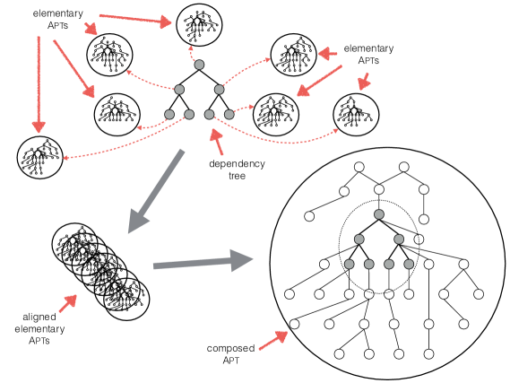
Figure 4: Composition of Apts.

As we have seen, the alignment of Apts can be achieved by adjusting the location of the anchor. The specific adjustments to the anchor locations are determined by the dependency tree for the phrase. For example, Figure 5 shows a dependency analysis of the phrase folded dry clothes. To align the elementary Apts for the lexemes in this tree, we do the following.

• The anchor of the elementary Apt for dry/JJ is moved to the node on which the bought/VBD and folded/VBD lie. This is the Apt shown at the top of Figure 6. This change of anchor location is determined by the path from the dry/JJ to folded/VBD in the tree in Figure 5, i.e. $\mbox{\small\sc{$\overline{\hbox{amod}}$}\/}\!\cdot\!\mbox{\small\sc{$\overline{\hbox{dobj}}$}\/}$.

• The anchor of the elementary Apt for clothes/NNS is moved to the node on which folded/VBD, hung/VBD and bought/VBD lie. This is the Apt shown at the bottom of Figure 3. This change of anchor location is determined by the path from the clothes/NNS to folded/VBD in the tree in Figure 5, i.e. $\overline{\hbox{dobj}}$.

• The anchor of the elementary Apt for folded/VBD has been left unchanged because there is an empty path from from the folded/VBD to folded/VBD in the tree in Figure 5.

[column sep=.0cm, row sep=.1ex] folded/VBD & dry/JJ & clothes/NNS
[edge unit distance=3ex]13dobj [edge unit distance=2ex]32amod

Figure 5: A dependency tree that generates the alignment shown in Figure 6.

Figure 6 shows the three elementary Apts for the lexemes dry/JJ, clothes/NNS and folded/VPD which have been aligned as determined by the dependency tree shown in Figure 5. Each column of lexemes appear at nodes that have been aligned with one another. For example, in the third column from the left, we see that the following three nodes have been aligned: (i) the node in the elementary Apt for dry/JJ at which bought/VBD and folded/VBD appear; (ii) the node in the elementary Apt for clothes/NNS at which folded/VBD, hung/VBD and bought/VBD appear; and (iii) the anchor node of the elementary Apt for folded/VBD, i.e the node at which folded/VBD appears. In the second phase of composition, these three nodes are merged together to produce a single node in the composed Apt.

[column sep=.0cm, row sep=.0ex] & & & & & & & & & & & & & & & & & & &
(a)& $\vdots$& we& bought& $\vdots$& $\vdots$& $\vdots$& $\vdots$& the& slightly& fizzy& wine& $\vdots$& $\vdots$& $\vdots$& $\vdots$& $\vdots$& $\vdots$& $\vdots$
& $\vdots$& $\vdots$& $\vdots$& $\vdots$& $\vdots$& $\vdots$& $\vdots$& $\vdots$& $\vdots$& dry& $\vdots$& $\vdots$& $\vdots$& $\vdots$& $\vdots$& $\vdots$& $\vdots$& $\vdots$
& $\vdots$& $\vdots$& $\vdots$& $\vdots$& $\vdots$& $\vdots$& $\vdots$& $\vdots$& $\vdots$& white& $\vdots$& $\vdots$& $\vdots$& $\vdots$& $\vdots$& $\vdots$& $\vdots$& $\vdots$

(b)& $\vdots$& $\vdots$& $\vdots$& $\vdots$& $\vdots$& $\vdots$& your& $\vdots$& $\vdots$& dry& joke& caused& laughter& $\vdots$& $\vdots$& $\vdots$& $\vdots$& $\vdots$
(c)& $\vdots$& he& folded& $\vdots$& $\vdots$& $\vdots$& $\vdots$& the& $\vdots$& clean& clothes& $\vdots$& $\vdots$& $\vdots$& $\vdots$& $\vdots$& $\vdots$& $\vdots$
& $\vdots$& $\vdots$& $\vdots$& $\vdots$& $\vdots$& $\vdots$& $\vdots$& $\vdots$& $\vdots$& dry& $\vdots$& $\vdots$& $\vdots$& $\vdots$& $\vdots$& $\vdots$& $\vdots$& $\vdots$&
(c)& $\vdots$& he& folded& $\vdots$& $\vdots$& $\vdots$& $\vdots$& the& $\vdots$& clean& clothes& $\vdots$& $\vdots$& $\vdots$& $\vdots$& $\vdots$& $\vdots$& $\vdots$&
& $\vdots$& $\vdots$& $\vdots$& $\vdots$& $\vdots$& $\vdots$& $\vdots$& $\vdots$& $\vdots$& dry& $\vdots$& $\vdots$& $\vdots$& $\vdots$& $\vdots$& $\vdots$& $\vdots$& $\vdots$&
(d)& $\vdots$& $\vdots$& $\vdots$& $\vdots$& $\vdots$& $\vdots$& your& $\vdots$& $\vdots$& $\vdots$& clothes& look& $\vdots$& great& $\vdots$& $\vdots$& $\vdots$& $\vdots$
(e)& the& man& hung& up& $\vdots$& $\vdots$& $\vdots$& the& $\vdots$& wet& clothes& $\vdots$& $\vdots$& $\vdots$& $\vdots$& $\vdots$& $\vdots$& $\vdots$
(f)& a& boy& bought& $\vdots$& $\vdots$& $\vdots$& $\vdots$& some& very& expensive& clothes& $\vdots$& $\vdots$& $\vdots$& $\vdots$& $\vdots$& $\vdots$& yesterday
(c)& $\vdots$& he& folded& $\vdots$& $\vdots$& $\vdots$& $\vdots$& the& $\vdots$& clean& clothes& $\vdots$& $\vdots$& $\vdots$& $\vdots$& $\vdots$& $\vdots$& $\vdots$
& $\vdots$& $\vdots$& $\vdots$& $\vdots$& $\vdots$& $\vdots$& $\vdots$& $\vdots$& $\vdots$& dry& $\vdots$& $\vdots$& $\vdots$& $\vdots$& $\vdots$& $\vdots$& $\vdots$& $\vdots$&
(g)& $\vdots$& she& folded& up& $\vdots$& $\vdots$& $\vdots$& $\vdots$& $\vdots$& $\vdots$& all& $\vdots$& $\vdots$& $\vdots$& of& the& laundry& $\vdots$
(h)& $\vdots$& he& folded& $\vdots$& under& pressure& $\vdots$& $\vdots$& $\vdots$& $\vdots$& $\vdots$& $\vdots$& $\vdots$& $\vdots$& $\vdots$& $\vdots$& $\vdots$& $\vdots$

& & & & & & & & & & & & & & & & & & &
[edge unit distance=2.5ex]32det [edge unit distance=2.5ex]43nsubj [edge unit distance=2.5ex]45prp [edge unit distance=2.0ex]412dobj [edge unit distance=2.5ex]129det [edge unit distance=2.7ex]128poss [edge unit distance=2.5ex]1110advmod [edge unit distance=2.5ex]1211amod [edge unit distance=2.5ex, color=lightgray, label style=draw=lightgray]1312nsubj [edge unit distance=2.7ex, color=lightgray, label style=draw=lightgray]1314dobj [edge unit distance=2.7ex, color=lightgray, label style=draw=lightgray]1315xcomp [edge unit distance=1.5ex]419tmod [edge unit distance=2.0ex]1218nmod [edge unit distance=2.5ex]1817det [edge unit distance=2.5ex]1816case [edge unit distance=2.5ex]47nmod [edge unit distance=2.5ex]76case

Figure 6: Vertically aligned Apts for dry/JJ, clothes/NNS and folded/VBD as determined by the tree in Figure 5. The letters in brackets on the left refer to the dependency trees shown in Figure 1 from which these Apts are constructed. For space reasons, part of speech tags have been omitted.

Before we discuss how the nodes in aligned Apts are merged, we formalize the notion of Apt alignment. We do this by first defining so-called offset Apts, which formalizes the idea of adjusting the location of an anchor. We then define how to align all of the Apts for the lexemes in a phrase based on a dependency tree.

4.2 Offset Apts

Given some offset, $\delta$, a string in $\hbox to0.0pt{\hskip 1.33507pt\leavevmode\hbox{\set@color$\overline{\hbox{}}$}\hss}{\leavevmode\hbox{\set@color$R$}}^{*}R^{*}$, the Apt $\mathbf{A}$ when offset by $\delta$ is denoted $\mathbf{A}^{\delta}$. Offsetting an Apt by $\delta$ involves moving the anchor to the position reached by following the path $\delta$ from the original anchor position. In order to define $\mathbf{A}^{\delta}$, we must define $\mathbf{A}^{\delta}(\tau,w^{\prime})$ for each $\tau\in\hbox to0.0pt{\hskip 1.33507pt\leavevmode\hbox{\set@color$\overline{\hbox{}}$}\hss}{\leavevmode\hbox{\set@color$R$}}^{*}R^{*}$ and $w^{\prime}\in V$, or in terms of our alternative tree-based representation, we need to specify the $\tau^{\prime}$ such that $\mathbf{A}^{\delta}(\tau)$ and $\mathbf{A}(\tau^{\prime})$ yield the same node (weighted lexeme multiset).

As shown in the Equation 7 below, path offset can be specified by making use of the co-occurrence type reduction operator that was introduced in Section 2.2. Given a string $\delta$ in $\hbox to0.0pt{\hskip 1.33507pt\leavevmode\hbox{\set@color$\overline{\hbox{}}$}\hss}{\leavevmode\hbox{\set@color$R$}}^{*}R^{*}$ and an Apt $\mathbf{A}$, the offset Apt $\mathbf{A}^{\delta}$ is defined as follows. For each $\tau\in\hbox to0.0pt{\hskip 1.33507pt\leavevmode\hbox{\set@color$\overline{\hbox{}}$}\hss}{\leavevmode\hbox{\set@color$R$}}^{*}R^{*}$ and $w\in V$:

$$\mathbf{A}^{\delta}(\tau,w)=\mathbf{A}(\downarrow\!({\delta\tau}),w)$$ (7)

or equivalently, for each $\tau\in\hbox to0.0pt{\hskip 1.33507pt\leavevmode\hbox{\set@color$\overline{\hbox{}}$}\hss}{\leavevmode\hbox{\set@color$R$}}^{*}R^{*}$:

$$\mathbf{A}^{\delta}(\tau)=\mathbf{A}(\downarrow\!({\delta\tau}))$$ (8)

As required, Equation 7 defines $\mathbf{A}^{\delta}$ by specifying the weighted lexeme multiset we get when $\mathbf{A}^{\delta}$ is applied to co-occurrence type $\tau$ as being the lexeme multiset that $\mathbf{A}$ produces when applied to the co-occurrence type $\downarrow\!({\delta\tau})$.

As an illustrative example, consider the Apt shown at the top of Figure 2. Let us call this Apt $\mathbf{A}$. Note that $\mathbf{A}$ is anchored at the node where the lexeme dry/JJ appears. Consider the Apt produced when we apply the offset $\mbox{\small\sc{$\overline{\hbox{amod}}$}\/}\!\cdot\!\mbox{\small\sc{$\overline{\hbox{dobj}}$}\/}$. This is shown at the top of Figure 3. Let us refer to this Apt as $\mathbf{A}^{\prime}$. The anchor of $\mathbf{A}^{\prime}$ is the node at which the lexemes bought/VDB and folded/VBD appear. Now we show how the two nodes $\mathbf{A}^{\prime}(\mbox{\small\sc nsubj\/})$ and $\mathbf{A}^{\prime}(\mbox{\small\sc dobj\/}\!\cdot\!\mbox{\small\sc amod\/}\!\cdot\!\mbox{\small\sc advmod\/})$ are defined in terms of $\mathbf{A}$ on the basis of Equation 8. In both cases the offset $\delta=\mbox{\small\sc{$\overline{\hbox{amod}}$}\/}\!\cdot\!\mbox{\small\sc{$\overline{\hbox{dobj}}$}\/}$.

• For the case where $\tau=\mbox{\small\sc nsubj\/}$ we have

  $$\begin{split}\mathbf{A}^{\prime}(\mbox{\small\sc nsubj\/})&=\mathbf{A}(\downarrow\!({\mbox{\small\sc{$\overline{\hbox{amod}}$}\/}\!\cdot\!\mbox{\small\sc{$\overline{\hbox{dobj}}$}\/}\!\cdot\!\mbox{\small\sc nsubj\/}}))\\ &=\mathbf{A}(\mbox{\small\sc{$\overline{\hbox{amod}}$}\/}\!\cdot\!\mbox{\small\sc{$\overline{\hbox{dobj}}$}\/}\!\cdot\!\mbox{\small\sc nsubj\/})\end{split}$$

  With respect to the anchor of $\mathbf{A}$, this correctly addresses the node at which the lexemes we/PRP and he/PRP appear.

• Where $\tau=\mbox{\small\sc dobj\/}\!\cdot\!\mbox{\small\sc amod\/}\!\cdot\!\mbox{\small\sc advmod\/}$ we have

  $$\begin{split}\mathbf{A}^{\prime}(\mbox{\small\sc dobj\/}\!\cdot\!\mbox{\small\sc amod\/}\!\cdot\!\mbox{\small\sc advmod\/})&=\mathbf{A}(\downarrow\!({\mbox{\small\sc{$\overline{\hbox{amod}}$}\/}\!\cdot\!\mbox{\small\sc{$\overline{\hbox{dobj}}$}\/}\!\cdot\!\mbox{\small\sc dobj\/}\!\cdot\!\mbox{\small\sc amod\/}\!\cdot\!\mbox{\small\sc advmod\/}}))\\ &=\mathbf{A}(\downarrow\!({\mbox{\small\sc{$\overline{\hbox{amod}}$}\/}\!\cdot\!\mbox{\small\sc amod\/}\!\cdot\!\mbox{\small\sc advmod\/}}))\\ &=\mathbf{A}(\downarrow\!({\mbox{\small\sc advmod\/}}))\\ &=\mathbf{A}(\mbox{\small\sc advmod\/})\end{split}$$

  With respect to the anchor of $\mathbf{A}$, this correctly addresses the node at which the lexeme slightly/RB appears.

In practice, the offset Apt $\mathbf{A}^{\delta}$ can be obtained by prepending the inverse of the path offset, $\delta^{-1}$, to all of the co-occurrence types in $\mathbf{A}$ and then repeatedly applying the reduction operator until no further reductions are possible. In other words, if $\tau$ addresses a node in $\mathbf{A}$, then $\tau^{\prime}$ addresses a node in $\mathbf{A}^{\delta}$ iff $\tau^{\prime}=\downarrow\!({\delta^{-1}\tau})$ and $\tau^{\prime}\in\hbox to0.0pt{\hskip 1.33507pt\leavevmode\hbox{\set@color$\overline{\hbox{}}$}\hss}{\leavevmode\hbox{\set@color$R$}}^{*}R^{*}$.

4.3 Syntax-driven Apt Alignment

We now make use of offset Apts, as defined in Equation 7, as a way to align all of the Apts associated with a dependency tree. Consider the following scenario:

• $w_{1}\ldots w_{n}$ is a the phrase (or sentence) where each $w_{i}\in V$ for $1\leq i\leq n$;

• $t\in T_{V,R}$ is a dependency analysis of the string $w_{1}\ldots w_{n}$;

• $w_{h}$ is the lexeme at the root of $t$. In other words, $h$ is the position (index) in the phrase at which the head appears;

• ${\|w_{i}\|}$ is the elementary Apt for $w_{i}$ for each $i$, $1\leq i\leq n$; and

• $\delta_{i}$, the offset of $w_{i}$ in $t$ with respect to the root, is the path in $t$ from $w_{i}$ to $w_{h}$. In other words, $\left\langle{w_{i}},\,{\delta_{i}},\,{w_{h}}\right\rangle$ is a co-occurrence in ${t}$ for each $i$, $1\leq i\leq n$. Note that $\delta_{h}=\epsilon$.

We define the distributional semantics for the tree $t$, denoted ${\|t\|}$, as follows:

$${\|t\|}=\bigsqcup{\left\{\,{{\|w_{1}\|{{}^{\delta_{1}}}},\ldots,{\|w_{n}\|{{}^{\delta_{n}}}}}\,\right\}}$$ (9)

The definition of $\bigsqcup$ is considered in Section 4.4. In general, $\bigsqcup$ operates on a set of $n$ aligned Apts, merging them into a single Apt. The multiset at each node in the resulting Apt is formed by merging $n$ multisets, one from each of the elements of $\left\{\,{{\|w_{1}\|{{}^{\delta_{1}}}},\ldots,{\|w_{n}\|{{}^{\delta_{n}}}}}\,\right\}$. It is this multiset merging operation that we focus on in Section 4.4.

Although ${\|t\|}$ can be taken to be the distributional semantics of the tree as a whole, the same Apt, when associated with different anchors (i.e. when offset in some appropriate way) provides a representation of each of the contextualized lexemes that appear in the tree.

For each $i$, for $1\leq i\leq n$, the Apt for $w_{i}$ when contextualized by its role in the dependency tree $t$, denoted ${\|w_{i};t\|}$, is the Apt that satisfies the equality:

$${\|w_{i};t\|}^{\delta_{i}}={\|t\|}$$ (10)

Alternatively, this can also be expressed with the equality:

$${\|w_{i};t\|}={\|t\|}^{{\delta_{i}}^{-1}}$$ (11)

Note that ${\|w_{h};t\|}$ and ${\|t\|}$ are identical. In other words, we take the representation of the distributional semantics of a dependency tree to be the Apt for the lexeme at the root of that tree that has been contextualized by the other lexemes appearing below it in the tree.

Equation 9 defined Apt composition as a “one-step” process in the sense that all of the $n$ elementary Apts that are associated with nodes in the dependency tree are composed at once to produce the resulting (composed) Apt. There are, however, alternative strategies that could be formulated. One possibility is fully incremental left-to-right composition, where, working left-to-right through the string of lexemes, the elementary Apts for the first two lexemes are composed, with the resulting Apt then being composed with the elementary Apt for the third lexeme, and so on. It is always possible to compose Apts in this fully incremental way, whatever the structure in the dependency tree. The tree structure, is however, critical in determining how the adjacent Apts need to be aligned.

4.4 Merging Aligned Apts

We now turn to the question of how to implement the function $\bigsqcup$ which appears in Equation 9. $\bigsqcup$ takes a set of $n$ aligned Apts, $\left\{\,{\mathbf{A}_{1},\ldots\mathbf{A}_{n}}\,\right\}$, one for each node in the dependency tree $t$. It merges the Apts together node by node to produce a single Apt, $\bigsqcup{\left\{\,{\mathbf{A}_{1},\ldots\mathbf{A}_{n}}\,\right\}}$, that represents the semantics of the dependency tree. Our discussion, therefore, addresses the question of how to merge the multisets that appear at nodes that are aligned with each other and form the nodes of the Apt being produced.

The elementary Apt for a lexeme expresses those co-occurrences that are distributionally compatible with the lexeme given the corpus. When lexemes in some phrase are composed, our objective is to capture the extent to which the co-occurrences arising in the elementary Apts are mutually compatible with the phrase as a whole. Once the elementary Apts that are being composed have been aligned, we are in a position to determine the extent to which co-occurrences are mutually compatible: co-occurrences that need to be compatible with one another are brought together through the alignment. We consider two alternative ways in which this can be achieved.

We begin with $\bigsqcup_{\textsc{int}}$ which provides a tight implementation of the mutual compatibility of co-occurrences. In particular, a co-occurrence is only deemed to be compatible with the composed lexemes to the extent that is distributionally compatible with the lexeme that it is least compatible with. This corresponds to the multiset version of intersection. In particular, for all $\tau\in\hbox to0.0pt{\hskip 1.33507pt\leavevmode\hbox{\set@color$\overline{\hbox{}}$}\hss}{\leavevmode\hbox{\set@color$R$}}^{*}R^{*}$ and $w^{\prime}\in V$:

$$\bigsqcup_{\textsc{int}}{\left\{\,{\mathbf{A}_{1},\ldots,\mathbf{A}_{n}}\,\right\}}(\tau,w^{\prime})=\min_{1\leq i\leq n}{\mathbf{A}_{i}(\tau,w^{\prime})}$$ (12)

It is clear that the effectiveness of $\bigsqcup_{\textsc{int}}$ increases as the size of $C$ grows, and that it would particularly benefit from distributional smoothing [Dagan, Pereira, and Lee,1994] which can be used to improve plausible co-occurrence coverage by inferring co-occurrences in the Apt for a lexeme $w$ based on the co-occurrences in the Apts of distributionally similar lexemes.

An alternative to $\bigsqcup_{\textsc{int}}$ is $\bigsqcup_{\textsc{uni}}$ where we determine distributional compatibility of a co-occurrence by aggregating across the distributional compatibility of the co-occurrence for each of the lexemes being composed. In particular, for all $\tau\in(\hbox to0.0pt{\hskip 1.33507pt\leavevmode\hbox{\set@color$\overline{\hbox{}}$}\hss}{\leavevmode\hbox{\set@color$R$}}\cup R)^{*}$ and $w^{\prime}\in V$:

$$\bigsqcup_{\textsc{uni}}{\left\{\,{\mathbf{A}_{1},\ldots,\mathbf{A}_{n}}\,\right\}}(\tau,w^{\prime})=\sum_{1\leq i\leq n}{\mathbf{A}_{i}(\tau,w^{\prime})}$$ (13)

While this clearly achieves co-occurrence embellishment, whether co-occurrence filtering is achieved depends on the weighting scheme being used. For example, if negative weights are allowed, then co-occurrence filtering can be achieved.

There is one very important feature of Apt composition that is a distinctive aspect of our proposal, and therefore worth dwelling on. In Section 4.1, when discussing Figure 4, we made reference to the notions of internal and external context. The internal context of a composed Apt is that part of the Apt that corresponds to the nodes in the dependency tree that generated the composed Apt. One might have expected that the only lexeme appearing at an internal node is the lexeme that appears at the corresponding node in the dependency tree. However, this is absolutely not the objective: at each node in the internal context, we expect to find a set of alternative lexemes that are, to varying degrees, distributionally compatible with that position in the Apt. We expect that a lexeme that is distributionally compatible with a substantial number of the lexemes being composed will result in a distributional feature with non-zero weight in the vectorized Apt. There is, therefore, no distinction being made between internal and external nodes. This enriches the distributional representation of the contextualized lexemes, and overcomes the potential problem arising from the fact that as larger and larger units are composed, there is less and less external context around to characterize distributional meaning.

5 Experiments

In this section we consider some empirical evidence in support of Apts. First, we consider some of the different ways in which Apts can be instantiated. Second, we present a number of case studies showing the disambiguating effect of Apt composition in adjective-noun composition. Finally, we evaluate the model using the phrase-based compositionality benchmarks of [Mitchell and Lapata,2008] and [Mitchell and Lapata,2010].

5.1 Instantiating Apts

We have constructed Apt lexicons from three different corpora.

• clean_wiki is a corpus used for the case studies in 5.2. This corpus is a cleaned 2013 Wikipedia dump [Wilson,2015] which we have tokenised, part-of-speech-tagged, lemmatised and dependency-parsed using the Malt Parser [Nivre,2004]. This corpus contains approximately 0.6 billion tokens.

• BNC is the British National Corpus. It has been tokenised, POS-tagged, lemmatised and dependency-parsed as described in [Grefenstette et al.,2013] and contains approximately 0.1 billion tokens.

• concat is a concatenation of the ukWaC corpus [Ferraresi et al.,2008], a mid-2009 dump of the English Wikipedia and the British National Corpus. This corpus has been tokenised, POS-tagged, lemmatised and dependency-parsed as described in [Grefenstette et al.,2013] and contains about 2.8 billion tokens.

Having constructed lexicons, there are a number of hyperparameters to be explored during composition. First there is the composition operation itself. We have explored variants which take a union of the features such as add and max and variants which take an intersection of the features such as mult, min and intersective_add, where intersective_add$(a,b)=a+b$ iff $a>0$ and $b>0$; $0$ otherwise.

Second, the Apt theory is agnostic to the type or derivation of the weights which are being composed. The weights in the elementary Apts can be counts, probabilities, or some variant of PPMI or other association function. Whilst it is generally accepted that the use of some association function such as PPMI is normally beneficial in the determination of lexical similarity, there is a choice over whether these weights should be seen as part of the representation of the lexeme, or as part of the similarity calculation. In the instantiation which we refer to as as compose_first, Apt weights are probabilities. These are composed and transformed to PPMI scores before computing cosine similarities. In the instantiation which we refer to as compose_second, Apt weights are PPMI scores.

There are a number of modifications that can be made to the standard PPMI calculation. First, it is common [Levy, Goldberg, and Dagan,2015] to delete rare words when building co-occurrence vectors. Low frequency features contribute little to similarity calculations because they co-occur with very few of the targets. Their inclusion will tend to reduce similarity scores across the board, but have little effect on ranking. Filtering, on the other hand, improves efficiency. In other experiments, we have found that a feature frequency threshold of $1000$ works well. On a corpus the size of Wikipedia ($~{}1.5$ billion tokens), this leads to a feature space for nouns of approximately $80,000$ dimensions (when including only first-order paths) and approximately $230,000$ dimensions (when including paths up to order $2$).

[Levy, Goldberg, and Dagan,2015] also showed that the use of context distribution smoothing (cds), $\alpha=0.75$, can lead to performance comparable with state-of-the-art word embeddings on word similarity tasks.

$$\mbox{{pmi}}_{\alpha}\left({w^{\prime}},{w};{\tau}\right)=\log\frac{\#{\left\langle{w},\,{\tau},\,{w^{\prime}}\right\rangle}\,\#{\left\langle{*},\,{\tau},\,{*}\right\rangle}^{\alpha}}{\#{\left\langle{w},\,{\tau},\,{*}\right\rangle}\,\#{\left\langle{*},\,{\tau},\,{w^{\prime}}\right\rangle}^{\alpha}}$$

[Levy, Goldberg, and Dagan,2015] further showed that using shifted PMI, which is analogous to the use of negative sampling in word embeddings, can be advantageous. When shifting PMI, all values are shifted down by $\log k$ before the threshold is applied.

$$\mbox{{sppmi}}\left({w^{\prime}},{w};{\tau}\right)=\max{(\mbox{{pmi}}\left({w^{\prime}},{w};{\tau}\right)-\log{k},0)}$$

Finally, there are many possible options for the path weighting function $\phi(\tau,w)$. These include the path probability $p({\tau}\,|\,{w})$ as discussed in Section 3, constant path weighting, and inverse path length or harmonic function (which is equivalent to the dynamic context window used in many neural implementations such as GloVe [Pennington, Socher, and Manning,2014]).

5.2 Disambiguation

Here we consider the differences between using aligned and unaligned Apt representations as well as the differences between using $\bigsqcup_{\textsc{uni}}$ and $\bigsqcup_{\textsc{int}}$ when carrying out adjective-noun (AN) composition. From the clean_wiki corpus described in Section 5.1, a small number of high frequency nouns were chosen which are ambiguous or broad in meaning together with potentially disambiguating adjectives. We use the compose_first option described above where composition is carried out on Apts containing probabilities.

$$\textsc{w}({w},\,\left\langle\,{\tau},{w^{\prime}}\,\right\rangle)=\frac{\#{\left\langle{w},\,{\tau},\,{w^{\prime}}\right\rangle}}{\#{\left\langle{w},\,{*},\,{*}\right\rangle}}$$

The closest distributional neighbours of the individual lexemes before and after composition with the disambiguating adjective are then examined. In order to calculate similarities, contexts are weighted using the variant of PPMI advocated by [Levy, Goldberg, and Dagan,2015] wherecds is applied with $\alpha=0.75$. However, no shift is applied to the PMI values since we have found shifting to have little or negative effect when working with relatively small corpora. Similarity is then computed using the standard cosine measure. For illustrative purposes the top ten neighbours of each word or phrase are shown, concentrating on ranks rather than absolute similarity scores.

	Aligned $\bigsqcup_{\textsc{uni}}$		Unaligned $\bigsqcup_{\textsc{uni}}$
shoot	green shoot	six-week shoot	green shoot	six-week shoot
shot     leaf   shooting   fight    scene   video    tour  footage  interview  flower	shoot     leaf   flower   fruit    orange   tree    color     shot   colour   cover	shoot     tour     shot     break   session   show   shooting concert interview   leaf	shoot     shot     leaf   shooting   fight    scene  video    tour     flower   footage	shoot     shot    shooting   leaf       scene   video   fight   footage   photo interview

Table 2: Neighbours of uncontextualised shoot/N compared to shoot/N in the contexts of green/J and six-week/J, using $\bigsqcup_{\textsc{uni}}$ with aligned and unaligned representations

	Aligned $\bigsqcup_{\textsc{int}}$		Unaligned $\bigsqcup_{\textsc{int}}$
shoot	green shoot	six-week shoot	green shoot	six-week shoot
shot     leaf   shooting   fight   scene  video   tour   flower   footage   interview	shoot       leaf       fruit    stalk   flower  twig   sprout     bud     shrub     inflorescence	shoot     photoshoot taping     tour     airing   rehearsal broadcast   session    q&a       post-production	shoot     pyrite   plosive   handlebars   annual   roundel   affricate   phosphor   connections reduplication	e/f     uemtsu     confederations shortlist   all-ireland   dern     gerwen   tactics backstroke     gabler

Table 3: Neighbours of uncontextualised shoot/N compared to shoot/N in the contexts of green/J and six-week/J, using $\bigsqcup_{\textsc{int}}$ with aligned and unaligned representations

Table 2 illustrates what happens when $\bigsqcup_{\textsc{uni}}$ is used to merge aligned and unaligned Apt representations when the noun shoot is placed in the contexts of green and six-week. Boldface is used in the entries of compounds where a neighbour appears to be highly suggestive of the intended sense and where it has a rank higher or equal to its rank in the entry for the uncontextualised noun. In this example, it is clear that merging the unaligned Apt representations provides very little disambiguation of the target noun. This is because typed co-occurrences for an adjective mostly belong in a different space to typed co-occurrences for a noun. Addition of these spaces leads to significantly lower absolute similarity scores, but little change in the ranking of neighbours. Whilst we only show one example here, this observation appears to hold true whenever words with different part of speech tags are composed. Intersection of these spaces via $\bigsqcup_{\textsc{int}}$ generally leads to substantially degraded neighbours, often little better than random, as illustrated by Table 3.

On the other hand when Apts are correctly aligned and merged using $\bigsqcup_{\textsc{uni}}$, we see the disambiguating effect of the adjective. A green shoot is more similar to leaf, flower, fruit and tree. A six-week shoot is more similar to tour, session, show and concert. This disambiguating effect is even more apparent when $\bigsqcup_{\textsc{int}}$ is used to merge the Apt representations (see Table 3).

	Aligned $\bigsqcup_{\textsc{uni}}$		Aligned $\bigsqcup_{\textsc{int}}$
group	musical group	ethnic group	musical group	ethnic group
group organization organisation company community corporation unit movement association society	group   company   band     music movement community society corporation category association	group organization organisation community company movement society     minority     unit     entity	group   band   troupe ensemble artist     trio     genre   music    duo     supergroup	group community organization grouping   sub-group faction ethnicity minority organisation tribe
body	human body	legislative body	human body	legislative body
body   board   organization entity   skin     head organisation   structure council   eye	body organization structure   entity  organisation skin     brain     eye     object   organ	body     council   committee board   authority assembly organisation agency commission entity	body   organism organization entity   embryo   brain community organelle institution cranium	body     council   committee board   legislature secretariat authority assembly power   office
work	social work	literary work	social work	literary work
study   project   book   activity   effort   publication job     program writing   piece	work   activity   study   project program practice development aspect   book   effort	work     book     study   novel   project   publication text     literature   story     writing	work     research   study     writings endeavour project discourse topic   development teaching	work     writings treatise     essay   poem     book     novel   monograph poetry   writing
field	athletic field	magnetic field	athletic field	magnetic field
facility   stadium   area   complex   ground   pool   base   space   centre   park	field     facility stadium gymnasium basketball sport   center  softball   gym   arena	field     component stadium     facility   track   ground   system   complex   parameter pool	field     gymnasium fieldhouse stadium   gym   arena   rink   softball cafeteria ballpark	field     wavefunction spacetime   flux     subfield     perturbation vector    e-magnetism formula_8   scalar

Table 4: Distributional Neighbors using $\bigsqcup_{\textsc{uni}}$ vs $\bigsqcup_{\textsc{int}}$ (e-magnetism = electro-magnetism)

Table 4 further illustrates the difference between using $\bigsqcup_{\textsc{uni}}$ and $\bigsqcup_{\textsc{int}}$ when composing aligned Apt representations. Again, boldface is used in the entries of compounds where a neighbour appears to be highly suggestive of the intended sense and where it has a rank higher or equal to its rank in the entry for the uncontextualised noun. In these examples, we can see that both $\bigsqcup_{\textsc{uni}}$ and $\bigsqcup_{\textsc{int}}$ appear to be effective in carrying out some disambiguation. Looking at the example of musical group, both $\bigsqcup_{\textsc{uni}}$ and $\bigsqcup_{\textsc{int}}$ increase the relative similarity of band and music to group when it is contextualised by musical. However, $\bigsqcup_{\textsc{int}}$ also leads to a number of other words being selected as neighbours which are closely related to the musical sense of group e.g. troupe, ensemble and trio. This is not the case when $\bigsqcup_{\textsc{uni}}$ is used — the other neighbours still appear related to the general meaning of group. This trend is also seen in some of the other examples such as ethnic group, human body and magnetic field. Further, even when $\bigsqcup_{\textsc{uni}}$ leads to the successful selection of a large number of sense specific neighbours, e.g. see literary work, the neighbours selected appear to be higher frequency, more general words than when $\bigsqcup_{\textsc{int}}$ is used.

The reason for this is likely to be the effect that each of these composition operations has on the number of non-zero dimensions in the composed representations. Ignoring the relatively small effect the feature association function may have on this, it is obvious that $\bigsqcup_{\textsc{uni}}$ should increase the number of non-zero dimensions whereas $\bigsqcup_{\textsc{int}}$ should decrease the number of non-zero dimensions. In general, the number of non-zero dimensions is highly correlated with frequency, which makes composed representations based on $\bigsqcup_{\textsc{uni}}$ behave like high frequency words and composed representations based on $\bigsqcup_{\textsc{int}}$ behave like low frequency words. Further, when using similarity measures based on PPMI, as demonstrated by [Weeds,2003], it is not unusual to find that the neighbours of high frequency entities (with a large number of non-zero dimensions) are other high frequency entities (also with a large number of non-zero dimensions). Nor is it unusual to find that the neighbours of low frequency entities (with a small number of non-zero dimensions) are other low frequency entities (with a small number of non-zero dimensions). [Weeds, Weir, and McCarthy,2004] showed that frequency is also a surprisingly good indicator of the generality of the word. Hence $\bigsqcup_{\textsc{uni}}$ leads to more general neighbours and $\bigsqcup_{\textsc{int}}$ leads to more specific neighbours.

Finally, note that whilst $\bigsqcup_{\textsc{int}}$ has produced high quality neighbours in these examples where only two words are composed, using $\bigsqcup_{\textsc{int}}$ in the context of the composition of an entire sentence would tend to lead to very sparse representations. The majority of the internal nodes of the Apt composed using an intersective operation such as $\bigsqcup_{\textsc{int}}$ must necessarily only include the lexemes actually used in the sentence. $\bigsqcup_{\textsc{uni}}$ on the other hand will have added to these internal representations, suggesting similar words which might have been used in those contexts and giving rise to a rich representation which might be used to calculate sentence similarity. Further, the use of PPMI, or some other similar form of feature weighting and selection, will mean that those internal (and external) contexts which are not supported by a majority of the lexemes in the sentence will tend to be considered insignificant and therefore will be ignored in similarity calculations. By using shifted PPMI, it should be possible to further reduce the number of non-zero dimensions in a representation constructed using $\bigsqcup_{\textsc{uni}}$ which should also allow us to control the specificity/generality of the neighbours observed.

5.3 Phrase-based Composition Tasks

Here we look at the performance of one instantiation of the Apt framework on two benchmark tasks for phrase-based composition.

5.3.1 Experiment 1: the M&L2010 dataset

The first experiment uses the M&L2010 dataset, introduced by [Mitchell and Lapata,2010], which contains human similarity judgements for adjective-noun (AN), noun-noun (NN) and verb-object (VO) combinations on a seven-point rating scale. It contains 108 combinations in each category such as $\langle\mbox{\em social activity},\mbox{\em economic condition}\rangle$, $\langle\mbox{\em tv set},\mbox{\em bedroom window}\rangle$ and $\langle\mbox{\em fight war},\mbox{\em win battle}\rangle$. This dataset has been used in a number of evaluations of compositional methods including [Mitchell and Lapata,2010], [Blacoe and Lapata,2012], [Turney,2012], [Hermann and Blunsom,2013] and [Kiela and Clark,2014]. For example, [Blacoe and Lapata,2012] show that multiplication in a simple distributional space (referred to here as an untyped VSM) outperforms the distributional memory (DM) method of [Baroni and Zamparelli,2010] and the neural language model (NLM) method of [Collobert and Weston,2008].

Whilst often not explicit, the experimental procedure in most of this work would appear to be the calculation of Spearman’s rank correlation coefficient $\rho$ between model scores and individual, non-aggregated, human ratings. For example, if there are 108 phrase pairs being judged by 6 humans, this would lead to a dataset containing 648 data points. The procedure is discussed at length in [Turney,2012], who argues that this method tends to underestimate model performance. Accordingly, Turney explicitly uses a different procedure where a separate Spearman’s $\rho$ is calculated between the model scores and the scores of each participant. These coefficients are then averaged to give the performance indicator for each model. Here, we report results using the original M&L method, see Table 5. We found that using the Turney method scores were typically higher by $0.01$ to $0.04$. If model scores are evaluated against aggregated human scores, then the values of Spearman’s $\rho$ tends to be still higher, typically $0.1$ to $0.12$ higher than the values reported here.

	AN	NN	VO	Average
$\bigsqcup_{\textsc{int}}$, $k=1$	-0.09	0.43	0.35	0.23
$\bigsqcup_{\textsc{int}}$, $k=10$	NaN	0.23	0.26	0.16
$\bigsqcup_{\textsc{uni}}$, $k=1$	0.47	0.37	0.40	0.41
$\bigsqcup_{\textsc{uni}}$, $k=10$	0.45	0.42	0.42	0.43
untyped VSM, multiply	0.46	0.49	0.37	0.44
[Mitchell and Lapata,2010]
untyped VSM, multiply	0.48	0.50	0.35	0.44
[Blacoe and Lapata,2012]
distributional memory (DM), add	0.37	0.30	0.29	0.32
[Blacoe and Lapata,2012]
neural language model (NLM), add	0.28	0.26	0.24	0.26
[Blacoe and Lapata,2012]
humans	0.52	0.49	0.55	0.52
[Mitchell and Lapata,2010]

Table 5: Results on the M&L2010 dataset using the M&L method of evaluation. Values shown are Spearman’s $\rho$.

For this experiment, we have constructed an order 2 Apt lexicon for the BNC corpus. This is the same corpus used by [Mitchell and Lapata,2010] and for the best performing algorithms in [Blacoe and Lapata,2012]. We note that the larger concat corpus was used by [Blacoe and Lapata,2012] in the evaluation of the DM algorithm [Baroni and Lenci,2010]. We use the compose_second option described above where the elementary Apt weights are PPMI. With regard to the different parameter settings in the PPMI calculation [Levy, Goldberg, and Dagan,2015], we tuned on a number of popular word similarity tasks: MEN [Bruni, Tran, and Baroni,2014]; WordSim-353 [Finkelstein et al.,2001]; and SimLex-999 [Hill, Reichart, and Korhonen,2015]. In these tuning experiments, we found that context distribution smoothing gave mixed results. However, shifting PPMI ($k=10$) gave optimal results across all of the word similarity tasks. Therefore we report results here for vanilla PPMI (shift $k=1$) and shifted PPMI (shift $k=10$). For composition, we report results for both $\bigsqcup_{\textsc{uni}}$ and $\bigsqcup_{\textsc{int}}$. Results are shown in Table 5.

For this task and with this corpus $\bigsqcup_{\textsc{uni}}$ consistently outperforms $\bigsqcup_{\textsc{int}}$. Shifting PPMI by $\log 10$ consistently improves results for $\bigsqcup_{\textsc{uni}}$, but has a large negative effect on the results for $\bigsqcup_{\textsc{int}}$. We believe that this is due to the relatively small size of the corpus. Shifting PPMI reduces the number of non-zero dimensions in each vector which increases the likelihood of a zero intersection. In the case of AN composition, all of the intersections were zero for this setting, making it impossible to compute a correlation.

Comparing these results with the state-of-the-art, we can see that $\bigsqcup_{\textsc{uni}}$ clearly outperforms DM and NLM as tested by [Blacoe and Lapata,2012]. This method of composition is also achieving close to the best results in [Mitchell and Lapata,2010] and [Blacoe and Lapata,2012]. It is interesting to note that our model does substantially better than the state-of-the-art on verb-object composition, but is considerably worse at noun-noun composition. Exploring why this is so is a matter for further research. We have undertaken experiments with a larger corpus and a larger range of hyper-parameter settings which indicate that the performance of the Apt models can be increased significantly. However, these results are not presented here, since an equatable comparison with existing models would require a similar exploration of the hyper-parameter space across all models being compared.

5.3.2 Experiment 2: the M&L2008 dataset

The second experiment uses the M&L2008 dataset, introduced by [Mitchell and Lapata,2008], which contains pairs of intransitive sensitives together with human judgments of similarity. The dataset contains 120 unique subject, verb, landmark triples with a varying number of human judgments per item. On average each triple is rated by 30 participants. The task is to rate the similarity of the verb and the landmark given the potentially disambiguating context of the subject. For example, in the context of the subject fire one might expect glowed to be close to burned but not close to beamed. Conversely, in the context of the subject face one might expect glowed to be close to beamed and not close to burned.

This dataset was used in the evaluations carried out by [Grefenstette et al.,2013] and [Dinu, Pham, and Baroni,2013]. These evaluations clearly follow the experimental procedure of Mitchell and Lapata and do not evaluate against mean scores. Instead, separate points are created for each human annotator, as discussed in Section 5.3.1.

The multi-step regression algorithm of [Grefenstette et al.,2013] achieved $\rho=0.23$ on this dataset. In the evaluation of [Dinu, Pham, and Baroni,2013], the lexical function algorithm, which learns a matrix representation for each functor and defines composition as matrix-vector multiplication, was the best performing compositional algorithm at this task. With optimal parameter settings, it achieved around $\rho=0.26$. In this evaluation, the full additive model of [Guevara,2010] achieved $\rho<0.05$.

In order to make our results directly comparable with these previous evaluations, we have used the same corpus to construct our Apt lexicons, namely the concat corpus described in Section 5.1. Otherwise, the Apt lexicon was constructed as described in Section 5.3.1. As before note that $k=1$ in shifted PPMI is equivalent to not shifting PPMI. Results are shown in Table 6.

$\bigsqcup_{\textsc{int}}$, $k=1$	0.23
$\bigsqcup_{\textsc{int}}$, $k=10$	0.13
$\bigsqcup_{\textsc{uni}}$, $k=1$	0.20
$\bigsqcup_{\textsc{uni}}$, $k=10$	0.26
multi-step regression	0.23
[Grefenstette et al.,2013]
lexical function	0.23–0.26
[Dinu, Pham, and Baroni,2013]
untyped VSM, mult	0.20-0.22
[Dinu, Pham, and Baroni,2013]
full additive	0–0.05
[Dinu, Pham, and Baroni,2013]
humans	0.40
[Mitchell and Lapata,2008]

Table 6: Results on the M&L2008 dataset. Values shown are Spearman’s $\rho$.

We see that $\bigsqcup_{\textsc{uni}}$ is highly competitive with the optimised lexical function model which was the best performing model in the evaluation of [Dinu, Pham, and Baroni,2013]. In that evaluation, the lexical function model achieved between 0.23 and 0.26 depending on the parameters used in dimensionality reduction. Using vanilla PPMI, without any context distribution smoothing or shifting, $\bigsqcup_{\textsc{uni}}$ achieves $\rho=0.20$, which is less than $\bigsqcup_{\textsc{int}}$. However, when using shifted PPMI as weights, the best result is $0.26$. The shifting of PPMI means that contexts need to be more surprising in order to be considered as features. This makes sense when using an additive model such as $\bigsqcup_{\textsc{uni}}$.

We also see that at this task and using this corpus $\bigsqcup_{\textsc{int}}$ performs relatively well. Using vanilla PPMI, without any context distribution smoothing or shifting, it achieves $\rho=0.23$ which equals the performance of the multi-step regression algorithm [Grefenstette et al.,2013]. Here, however, shifting PPMI has a negative impact on performance. This is largely due to the intersective nature of the composition operation — if shifting PPMI removes a feature from one of the unigram representations, it cannot be recovered during composition.

6 Related Work

Our work brings together two strands usually treated as separate though related problems: representing phrasal meaning by creating distributional representations through composition; and representing word meaning in context by modifying the distributional representation of a word. In common with some other work on lexical distributional similarity, we use a typed co-occurrence space. However, we propose the use of higher-order grammatical dependency relations to enable the representation of phrasal meaning and the representation of word meaning in context.

6.1 Representing Phrasal Meaning

The problem of representing phrasal meaning has traditionally been tackled by taking vector representations for words [Turney and Pantel,2010] and combining them using some function to produce a data structure that represents the phrase or sentence. Mitchell and Lapata (2008, 2010) found that simple additive and multiplicative functions applied to proximity-based vector representations were no less effective than more complex functions when performance was assessed against human similarity judgements of simple paired phrases.

The word embeddings learnt by the continuous bag-of-words model (CBOW) and the continuous skip-gram model proposed by Mikolov et al. (2013a, 2013b) are currently among the most popular forms of distributional word representations. Whilst using a neural network architecture, the intuitions behind such distributed representations of words are the same as in traditional distributional representations. As argued by Pennington et al. (2014), both count-based and prediction-based models probe the underlying corpus co-occurrences statistics. For example, the CBOW architecture predicts the current word based on context (which is viewed as a bag-of-words) and the skip-gram architecture predicts surrounding words given the current word. Mikolov et al. (2013c) showed that it is possible to use these models to efficiently learn low-dimensional representations for words which appear to capture both syntactic and semantic regularities. [Mikolov et al.,2013b] also demonstrated the possibility of composing skip-gram representations using addition. For example, they found that adding the vectors for Russian and river results in a very similar vector to the result of adding the vectors for Volga and river. This is similar to the multiplicative model of [Mitchell and Lapata,2008] since the sum of two skip-gram word vectors is related to the product of two word context distributions.

Whilst our model shares with these the use of vector addition as a composition operation, the underlying framework is very different. Specifically, the actual vectors added depend not just on the form of the words but also their grammatical relationship within the phrase or sentence. This means that the representation for, say, glass window is not equal to the representation of window glass. The direction of the nn relationship between the words leads to a different alignment of the Apts and consequently a different representation for the phrases.

There are other approaches which incorporate theoretical ideas from formal semantics and machine learning, use syntactic information, and specialise the data structures to the task in hand. For adjective-noun phrase composition, [Baroni and Zamparelli,2010] and [Guevara,2010] borrowed from formal semantics the notion that an adjective acts as a modifying function on the noun. They represented a noun as a vector, an adjective as a matrix, which could be induced from pairs of nouns and adjective noun phrases, and composed the two using matrix-by-vector multiplication to produce a vector for the noun phrase. Separately, [Coecke, Sadrzadeh, and Clark,2011] proposed a broader compositional framework that incorporated from formal semantics the notion of function application derived from syntactic structure [Montague,1970, Lambek,1999]. These two approaches were subsequently combined and extended to incorporate simple transitive and intransitive sentences, with functions represented by tensors, and arguments represented by vectors [Grefenstette et al.,2013].

The MV-RNN model of [Socher et al.,2012] broadened the [Baroni and Zamparelli,2010] approach; all words, regardless of part-of-speech, were modelled with both a vector and a matrix. This approach also shared features with [Coecke, Sadrzadeh, and Clark,2011] in using syntax to guide the order of phrasal composition. This model, however, was made much more flexible by requiring and using task-specific labelled training data to create task-specific distributional data structures, and by allowing non-linear relationships between component data structures and the composed result. The payoff for this increased flexibility has come with impressive performance in sentiment analysis [Socher et al.,2012, Socher et al.,2013].

However, whilst these approaches all pay attention to syntax, they all require large amounts of training data. For example, running regression models to accurately predict the matrix or tensor for each individual adjective or verb requires a large number of exemplar compositions containing that adjective or verb. Socher’s MV-RNN model further requires task-specific labelled training data. Our approach, on the other hand, is purely count-based and directly aggregates information about each word from the corpus.

Other approaches have been proposed. Clarke (2007, 2012) suggested a context-theoretic semantic framework, incorporating a generative model that assigned probabilities to arbitrary word sequences. This approach shared with [Coecke, Sadrzadeh, and Clark,2011] an ambition to provide a bridge between compositional distributional semantics and formal logic-based semantics. In a similar vein, [Garrette, Erk, and Mooney,2011] combined word-level distributional vector representations with logic-based representation using a probabilistic reasoning framework. [Lewis and Steedman,2013] also attempted to combine distributional and logical semantics by learning a lexicon for CCG (Combinatory Categorial Grammar [Steedman,2000]) which first maps natural language to a deterministic logical form and then performs a distributional clustering over logical predicates based on arguments. The CCG formalism was also used by [Hermann and Blunsom,2013] as a means for incorporating syntax-sensitivity into vector space representations of sentential semantics based on recursive auto-encoders (Socher et al. (2011a, 2011b)). They achieved this by representing each combinatory step in a CCG parse tree with an auto-encoder function, where it is possible to parameterise both the weight matrix and bias on the combinatory rule and the CCG category.

[Turney,2012] offered a model that incorporated assessments of word-level semantic relations in order to determine phrasal-level similarity. This work uses two different word-level distributional representations to encapsulate two types of similarity, and captures instances where the components of a composed noun phrase bore similarity to another word through a mix of those similarity types. Crucially, it views similarity of phrases as a function of the similarities of the components and does not attempt to derive modified vectors for phrases or words in context. [Dinu and Thater,2012] also compared computing sentence similarity via additive compositional models with an alignment-based approach, where sentence similarity is a function of the similarities of component words, and simple word overlap. Their results showed that a model based on a mixture of these approaches outperformed all of the individual approaches on a number of textual entailment datasets.

6.2 Typed Co-occurrence Models

In untyped co-occurrence models, such as those considered by Mitchell and Lapata (2008, 2010) , co-occurrences are simple, untyped pairs of words which co-occur together (usually within some window of proximity but possibly within some grammatical relation). The lack of typing makes it possible to compose vectors through addition and multiplication. However, in the computation of lexical distributional similarity using grammatical dependency relations, it has been typical [Lin,1998, Lee,1999, Weeds and Weir,2005] to consider the type of a co-occurrence (for example, does dog occur with eat as its direct object or its subject?) as part of the feature space. The distinction between vector spaces based on untyped and typed co-occurrences was formalised by [Padó and Lapata,2007] and [Baroni and Lenci,2010]. In particular, [Baroni and Lenci,2010] showed that typed co-occurrences based on grammatical relations were better than untyped co-occurrences for distinguishing certain semantic relations. However, as shown by [Weeds, Weir, and Reffin,2014], it does not make sense to compose typed features based on first-order dependency relations through multiplication and addition, since the vector spaces for different parts of speech are largely non-overlapping.

[Padó and Lapata,2007] constructed features using higher-order grammatical dependency relations. They defined a path through a dependency tree in terms of the node words. This allowed words which are only indirectly related within a sentence to be considered as co-occurring. For example, in a lorry carries apples, there is a path of length 2 between the nouns lorry and apples via the node carry. However, they also used a word-based basis mapping which essentially reduces all of the salient grammatical paths to untyped co-occurrences. Given the paths $\langle\mbox{\em lorry},\mbox{\em carry}\rangle$ and $\langle\mbox{\em lorry},\mbox{\em carry},\mbox{\em apples}\rangle$ for lorry, these would be mapped to the basis elements carry and apples respectively.

6.3 Representing Word Meaning in Context

A long-standing topic in distributional semantics has been the modification of a canonical representation of a lexeme’s meaning to reflect the context in which it is found. Typically, a canonical vector for a lexeme is estimated from all corpus occurrences and the vector then modified to reflect the instance context [Lund and Burgess,1996, Erk and Padó,2008, Mitchell and Lapata,2008, Thater, Dinu, and Pinkal,2009, Thater, Fürstenau, and Pinkal,2010, Thater, Fürstenau, and Pinkal,2011, Van de Cruys, Poibeau, and Korhonen,2011, Erk,2012].

As described in Mitchell and Lapata (2008, 2010), lexeme vectors have typically been modified using simple additive and multiplicative compositional functions. Other approaches, however, share with our proposal the use of syntax to drive modification of the distributional representation [Erk and Padó,2008, Thater, Dinu, and Pinkal,2009, Thater, Fürstenau, and Pinkal,2010, Thater, Fürstenau, and Pinkal,2011].

[Erk and Padó,2008] introduced a structured vector space model of word meaning that computes the meaning of a word in the context of another word via selectional preferences. This approach was shown to work well at ranking paraphrases taken from the SemEval-2007 lexical substitution task [McCarthy and Navigli,2007]. In the Erk & Padó approach, the meaning of ball in the context of the phrase catch ball is computed by combining the lexical vector for ball with the object preference vector of catch i.e. things which can be caught. Whilst this approach is based on very similar intuitions to ours, it is in fact quite different. The lexical vector which is modified is not the co-occurrence vector, as in our model, but a vector of neighbours computed from co-occurrences. For example, the lexical vector for catch in the Erk & Padó approach might contain throw, catch and organise. These neighbours of catch are then combined with verbs which have been seen with ball in the direct object relation using vector addition or component-wise multiplication. Thus, it is possible to carry out this approach with reference only to observed first order grammatical dependency relationship. In their experiments, they used the “dependency-based” vector space of [Padó and Lapata,2007] where target and context words are linked by a valid dependency path (i.e. not necessarily a single first-order grammatical relation). However, higher-order dependency paths were purely used to provide extra contexts for target words, than would be seen in a traditional first-order dependency model, during the computation of neighbour sets. Further, the Erk & Padó approach does not construct a representation of the phrase since this model is focussed on lexical disambiguation rather than composition and it is not obvious how one would carry out further disambiguations within the context of a whole sentence.

More recently, [Thater, Fürstenau, and Pinkal,2011] used a similar approach but considered a broader range of operations for combining two vectors where individual vector components are reweighted. Specifically, they found that reweighting vector components based on the distributional similarity score between words defining vector components and the observed context words led to improved performance at ranking paraphrases.

[Thater, Fürstenau, and Pinkal,2010] noted that vectors of two syntactically related words typically have different syntactic environments, making it difficult to combine information in the respective vectors. They build on [Thater, Dinu, and Pinkal,2009], where the meaning of argument nouns was modelled in terms of the predicates they co-occur with (referred to as a first-order vector) and the meaning of predicates in terms of second-order co-occurrence frequencies with other predicates. These predicate vectors can be obtained by adding argument vectors. For example, the verb catch will contain counts on the dimension for kick introduced by the direct-object ball and counts on the dimension for contract introduced by the direct-object cold. In other words, like in the Erk & Padó approach, the vector for a verb can be seen as a vector of similar verbs, thus making this notion of second-order dependency compatible with that used in work on word sense discrimination [Schütze,1998] rather than referring to second-order (or higher order) grammatical dependencies as in this work. Contextualisation can then be achieved by multiplication of a second-order predicate vector with a first-order argument vector since this selects the dimensions which are common to both. [Thater, Fürstenau, and Pinkal,2010] presented a more general model where every word is modelled in terms of first-order and second-order co-occurrences and demonstrate high performance at ranking paraphrases.

7 Directions for Future Work

7.1 Representations

There are a number of apparent limitations of our approach that are simply a reflection of our decision to adopt dependency-based syntactic analysis.

First, surface disparities in syntactic structure (e.g. active versus passive tense formations, compound sentence structures) will disrupt sentence-level comparisons using a simple Apt structure based on surface dependency relations, but this can be addressed, for example, by syntax-based pre-processing. The Apt approach is agnostic in this regard.

Second, traditional dependency parsing does not distinguish between the order of modifiers. Hence the phrases happiest blonde person and blonde happiest person receive the same dependency representation and therefore also the same semantic representation. However, we believe that our approach is flexible enough to be able to accommodate a more sensitive grammar formalism which does allow for distinctions in modifier scope to be made if an application demands it. In future work we intend to look at other grammar formalisms including CCG [Steedman,2000].

By proposing a count-based method for composition we are bucking the growing trend of working with prediction-based word embeddings. Whilst there has been initial evidence [Baroni, Dinu, and Kruszewski,2014] that prediction-based methods are superior to count-based methods at the lexeme level e.g. for synonym detection and concept categorisation, it has also been shown [Levy and Goldberg,2014] that the skip-gram model with negative sampling as introduced in [Mikolov et al.,2013a] is equivalent to implicit factorisation of the PPMI matrix. [Levy, Goldberg, and Dagan,2015] also demonstrated how traditional count-based methods could be improved by transferring hyperparameters used by the prediction-based methods (such as context distribution smoothing and negative sampling). This led to the count-based methods outperforming the prediction-based methods on a number of word similarity tasks. A next step for us is to take the lessons learnt from work on word embeddings and find a way to produce lower dimensionality Apt representations without destroying the necessary structure which drives composition. The advantages of this from a computational point of view are obvious. It remains to be seen what effect the improved generalization also promised by dimensionality reduction will have on composition via Apts.

By considering examples, we have seen that composition of Apts using both union and intersection can lead to nearest neighbours which are clearly disambiguating. On benchmark phrase-based composition tasks, the performance of union in Apt composition is close to or equalling the state-of-the-art on those tasks. However, we believe that the performance of intersection in Apt composition is currently limited by the impoverished nature of word representations based directly on corpus statistics. Even given a very large corpus, there are always many plausible co-occurrences which have not been observed. One possible solution, which we explore elsewhere, is to smooth the word representations using their distributional neighbours before applying an intersective composition operation.

7.2 Applications

In Section 5.2, we demonstrated the potential for using Apts to carry out word sense disambiguation / induction. Uncontextualised, elementary Apts typically contain a corpus-determined mixture of co-occurrences referencing different usages. The Apt generated by a dependency tree, however, provides contextualised lexeme representations where the weights have been adjusted by the influence of the contextual lexemes so that the co-occurrences relating to the correct usage have been appropriately up-weighted, and the co-occurrences found in other circumstances down-weighted. In other words, Apt structures automatically perform word sense induction on lexeme-level representations which is demonstrable through the lexeme similarity measure. For example, we observed that the contextualised lexeme representation of body in the Apt constructed by embedding it in the phrase human body had a relatively high similarity to the uncontextualised representation of brain and a relatively low similarity to council, while the equivalent lexeme representation for body embedded in the Apt constructed for the phrase legislative body showed the reverse pattern.

One common criticism of distributional thesauruses is that they conflate different semantic relations into a single notion of similarity. For example, when comparing representations based on grammatical dependency relations, the most similar word to an adjective such as hot will usually be found to be its antonym cold. This is because hot and cold are both used to modify many of the same nouns. However, if as in the Apt framework, the representation of cold includes not only the direct dependents of cold, but also the indirect dependents, e.g. verbs which co-occur with cold things, it is possible that more differences between its representation and that of hot might be found. One would imagine that the things which are done to hot things are more different to the things which are done to cold things than they are to the things which are done to very warm things. Further, the examples in Section 5.2 raises the possibility that different composition operations might be used to distinguish different semantic relations including hypernyms, hyponyms and co-hyponyms. For example, $\bigsqcup_{\textsc{uni}}$ tends to lead to more general neighbours (e.g. hypernyms) and $\bigsqcup_{\textsc{int}}$ tends to lead to more specific neighbours (e.g. hyponyms).

Phrase-level or sentence-level plausibility measures offer the prospect of a continuous measure of the appropriateness / plausibility of a complete phrase or sentence, based on a combination of semantic and syntactic dependency relations. Apts offer a way to measure the plausibility of a lexeme when embedded in a dependency tree, suggesting that Apts may be successfully employed in tackling sentence completion tasks, such as the Microsoft Research Sentence Completion Challenge [Zweig and Burges,2012]. Here the objective is to identify the word that will fill out a partially completed sentence in the best possible way. For example, is flurried or profitable the best completion of the sentence below.

”Presently he emerged looking even more [flurried / profitable] than before.”

We can compose the Apts for the partially completed sentence. Comparing the result with the elementary Apts for each of the candidates should provide a good, direct measurement of which candidate is more plausible. An improved language model has implications for parsing, speech recognition and machine translation.

A central goal of compositional distributional semantics is to create a data structure that represents an entire phrase or sentence. The composed Apt for a dependency tree provides such a structure, but leaves open the question as to how this structure might be exploited for phrase-level or sentence-level semantic comparison.

The first point to be made is that, unusually, we have available not only a representation of the whole dependency tree but also contextualised (vector) representations for the lexemes in the dependency tree. This makes available to us any analytical technique which requires separate analysis of lexical components of the phrase or sentence. However, this leads to the problem of how to read the structure at the global phrase/sentence-level.

For similarity measures, one straightforward option would be to create a vector from the Apt anchored at the head of the phrase or sentence being considered. Thus the phrasal vector for a red rose would be created taking the node containing rose as the anchor. In other words, the vector representation of the phrase a red rose will be the same as the contextualised representation of rose. Similarly, the vector representation for the sentence he took the dog for a walk will be the same as the contextualised representation of the verb took.

Such a representation provides a continuous model of similarity (and meaning) at the phrasal-level and/or sentence-level. We anticipate that vector comparisons of phrase or sentence-level vectors produced in this manner will provide some coherent numerical measure of distributional similarity. This approach should be useful for paraphrase recognition tasks. For example, in order to identify good candidate paraphrases for questions in a question-answering task, [Berant and Liang,2014] employ a paraphrase model based on adding word embeddings constructed using the CBOW model of Mikolov et al. (2013). Whilst the authors achieve state-of-the-art using a mixture of methods, a paraphrase model based on the addition of vectors of untyped co-occurrences alone cannot distinguish meanings where syntax is important. For example, the sentences Oswald shot Kennedy and Kennedy shot Oswald would have the same representations. On the other hand, Apt composition is syntax-driven and will provide a representation of each sentence which is sensitive to lexical meaning and syntax.

Another advantage of using Apt composition in paraphrase recognition, over some other syntax-driven proposals, is that the same structure is used to represent words, phrases and sentences. Provided the head node is of the same type of speech, words and phrases of different lengths can easily be compared within our model. An adjective-noun compound such as male sibling is directly comparable with the single noun brother. Further, there is no need for there to be high similarity between aligned components of phrases or sentences. For example, the phrase female scholar can be expected to have a high similarity with the phrase educated woman, in terms at least of their external contexts.

8 Conclusions

This paper presents a new theory of compositional distributional semantics. It employs a single structure, the Apt, which can represent the distributional semantics of lexemes, phrases and even sentences. By retaining higher-order grammatical structure in the representations of lexemes, composition captures mutual disambiguation and mutual generalisation of constituents. Apts allow lexemes and phrases to be compared in isolation or in context. Further, we have demonstrated how one instantiation of this theory can achieve results which are very competitive with state-of-the-art results on benchmark phrase-based composition tasks.

As we have discussed, Apts have a wide range of potential applications including word sense induction, word sense disambiguation, parse reranking, dependency parsing and language modelling more generally, and also paraphrase recognition. Further work is required to gain an understanding of which instantiations of the theory are suited to each of these applications.

9 Acknowledgements

This work was funded by UK EPSRC project EP/IO37458/1 “A Unified Model of Compositional and Distributional Compositional Semantics: Theory and Applications”. We would like to thank all members of the DISCO project team. Particular thanks to Miroslav Batchkarov, Stephen Clark, Daoud Clarke, Roland Davis, Bill Keller, Tamara Polajnar, Laura Rimell, Mehrnoosh Sadrzadeh, David Sheldrick and Andreas Vlachos. We would also like to thank the anonymous reviewers for their helpful comments.

References

- [Baroni, Dinu, and Kruszewski,2014] Baroni, Marco, Georgiana Dinu, and Germán Kruszewski. 2014. Don’t count, predict! a systematic comparison of context-counting vs. context-predicting semantic vectors. In Proceedings of the 52nd Annual Meeting of the Association for Computational Linguistics (Volume 1: Long Papers), pages 238–247, Baltimore, Maryland, June. Association for Computational Linguistics.
- [Baroni and Lenci,2010] Baroni, Marco and Alessandro Lenci. 2010. Distributional memory: A general framework for corpus-based semantics. Computational Linguistics, 36(4):673–721, dec.
- [Baroni and Zamparelli,2010] Baroni, Marco and Roberto Zamparelli. 2010. Nouns are vectors, adjectives are matrices: Representing adjective-noun constructions in semantic space. In Proceedings of the 2010 Conference on Empirical Methods in Natural Language Processing, pages 1183–1193, Cambridge, MA, October. Association for Computational Linguistics.
- [Berant and Liang,2014] Berant, Jonathan and Percy Liang. 2014. Semantic parsing via paraphrasing. In Proceedings of the 52nd Annual Meeting of the Association for Computational Linguistics (Volume 1: Long Papers), pages 1415–1425, Baltimore, Maryland. Association for Computational Linguistics.
- [Blacoe and Lapata,2012] Blacoe, William and Mirella Lapata. 2012. A comparison of vector-based representations for semantic composition. In Proceedings of the 2012 Joint Conference on Empirical Methods in Natural Language Processing and Computational Natural Language Learning, pages 546–556, Jeju Island, Korea, July. Association for Computational Linguistics.
- [Bruni, Tran, and Baroni,2014] Bruni, Elia, Nam Khanh Tran, and Marco Baroni. 2014. Multimodal distributional semantics. Journal of Artificial Intelligence Research, 49:1–47.
- [Clarke,2007] Clarke, Daoud. 2007. Context-theoretic Semantics for Natural Language: an Algebraic Framework. Ph.D. thesis, Department of Informatics, University of Sussex.
- [Clarke,2012] Clarke, Daoud. 2012. A context-theoretic framework for compositionality in distributional semantics. Computational Linguistics, 38.
- [Coecke, Sadrzadeh, and Clark,2011] Coecke, Bob, Mehrnoosh Sadrzadeh, and Stephen Clark. 2011. Mathematical foundations for a compositional distributed model of meaning. Linguistic Analysis, 36(1-4):345–384.
- [Collobert and Weston,2008] Collobert, Ronan and Jason Weston. 2008. A unified architecture for natural language processing: Deep neural networks with multitask learning. In Proceedings of the 25th International Conference on Machine Learning, ICML ’08, pages 160–167, New York, NY, USA. ACM.
- [Curran,2004] Curran, James. 2004. From Distributional to Semantic Similarity. Ph.D. thesis, University of Edinburgh.
- [Dagan, Pereira, and Lee,1994] Dagan, Ido, Fernando Pereira, and Lillian Lee. 1994. Similarity-based estimation of word cooccurrence probabilities. In Proceedings of the 32nd Annual Meeting of the Association for Computational Linguistics, pages 272–278, Las Cruces, New Mexico, USA, June. Association for Computational Linguistics.